paul krugman’s new economic geography: past, present and ...klufova/spatial_economy/thisse.pdf ·...
TRANSCRIPT

J.-F. ThisseCORE-UCLouvain (Belgium)
Paul Krugman’s New Economic Geography: past, present and future
Paul Krugman’s New Economic Geography: past, present and future

Economic geography seeks toexplain the riddle of unequal
spatial development
(at different spatial scales)
2

C o u n trie s 1 8 0 0 1 8 3 0 1 8 5 0 1 8 7 0 1 8 9 0 1 9 0 0 1 9 1 3A u s tr ia -H u n ga ry 2 0 0 2 4 0 2 7 5 3 1 0 3 7 0 4 2 5 5 1 0B e lgiu m 2 0 0 2 4 0 3 3 5 4 5 0 5 5 5 6 5 0 8 1 5B u lga r ia 1 7 5 1 8 5 2 0 5 2 2 5 2 6 0 2 7 5 2 8 5D e n m a rk 2 0 5 2 2 5 2 8 0 3 6 5 5 2 5 6 5 5 8 8 5F in la n d 1 8 0 1 9 0 2 3 0 3 0 0 3 7 0 4 3 0 5 2 5F ra n c e 2 0 5 2 7 5 3 4 5 4 5 0 5 2 5 6 1 0 6 7 0G e rm a n y 2 0 0 2 4 0 3 0 5 4 2 5 5 4 0 6 4 5 7 9 0G re e c e 1 9 0 1 9 5 2 2 0 2 5 5 3 0 0 3 1 0 3 3 5I ta ly 2 2 0 2 4 0 2 6 0 3 0 0 3 1 5 3 4 5 4 5 5N e th e r la n d s 2 7 0 3 2 0 3 8 5 4 7 0 5 7 0 6 1 0 7 4 0N o rw a y 1 8 5 2 2 5 2 8 5 3 4 0 4 3 0 4 7 5 6 1 5P o r tu ga l 2 3 0 2 5 0 2 7 5 2 9 0 2 9 5 3 2 0 3 3 5R o m a n ia 1 9 0 1 9 5 2 0 5 2 2 5 2 6 5 3 0 0 3 7 0R u ss ia 1 7 0 1 8 0 1 9 0 2 2 0 2 1 0 2 6 0 3 4 0S e rb ia 1 8 5 2 0 0 2 1 5 2 3 5 2 6 0 2 7 0 3 0 0S p a in 2 1 0 2 5 0 2 9 5 3 1 5 3 2 5 3 6 5 4 0 0S w e d e n 1 9 5 2 3 5 2 7 0 3 1 5 4 0 5 4 9 5 7 0 5S w itz e r la n d 1 9 0 2 4 0 3 4 0 4 8 5 6 4 5 7 3 0 8 9 5U n ite d K in gd o m 2 4 0 3 5 5 4 7 0 6 5 0 8 1 5 9 1 5 1 0 3 5
M e a n 1 9 9 2 4 0 2 8 5 3 5 0 4 0 0 4 6 5 5 5 0S ta n d a rd -d e v ia t io n 2 4 4 3 6 8 1 1 0 1 5 5 1 8 2 2 2 9
U n ite d S ta te s 2 4 0 3 2 5 4 6 5 5 8 0 8 7 5 1 0 7 0 1 3 5 03

Does Geography Matter?
“transport costs are almost universally ignored in trade
models in the sanguine hope that if included they would not
materially affect the results”(Deardorff)
4
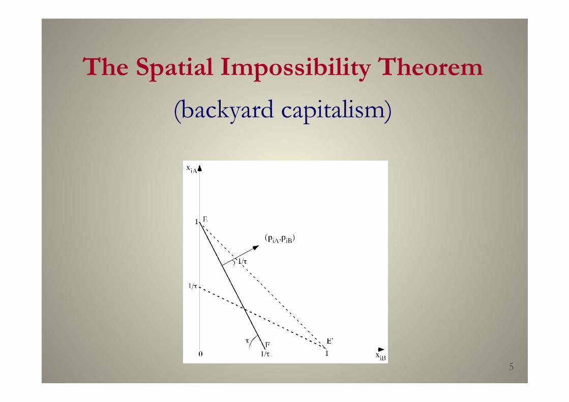
The Spatial Impossibility Theorem(backyard capitalism)
5

What Are the Alternative Strategies?
- Comparative advantage (monocentric city)
6
- Agglomeration externalities (spillover effects)
- Imperfect competition(i) oligopolistic competition (spatial competition)(ii) monopolistic competition (Dixit-Stiglitz)

The Beginnings of NEG
7
The Principle of Differentiation
The Home Market Effect

Agglomeration at the market centeris a Nash equilibrium if t ⁄ 2μ ≤ 1
The Principle of Differentiation
8
Spatial differentiation relaxes price competition
Pi(x) ≡exp −(pi + t |x − yi |) /µ
exp−(p j + t |x − y j |) /µj=1
n∑

The Home Market Effect
Two regions: H is bigger than F
Two production factors: (immobile) labor and (mobile) capital
Two production sectors
Using labor, one sector operates under constant returns, perfect competition and zero trade costs
Using labor and capital, the sector operates under increasingreturns, monopolistic competition and positive trade costs
9
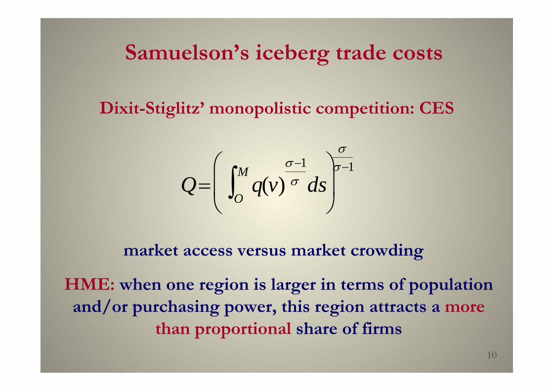
Samuelson’s iceberg trade costs
market access versus market crowding
Dixit-Stiglitz’ monopolistic competition: CES
HME: when one region is larger in terms of population and/or purchasing power, this region attracts a more
than proportional share of firms
Q= q(v)σ −1σ
O
M∫ ds⎛
⎝ ⎜
⎞
⎠ ⎟
σσ −1
10

HME: when one region is larger in terms of population and/or
purchasing power, this region attracts a more
than proportional share of firms
11
an initial size advantage is magnifiedby trade liberalization

The Core-periphery Structure
12
or when physical capital is replaced by human capital
when workers move to a new place, they bring with them both their
production and consumption capabilities

13
there is circular causation (à la Myrdal) :“manufactures production will tend to concentrate
where there is a large market, but the market will be large where manufactures production is concentrated”
(Krugman)
14
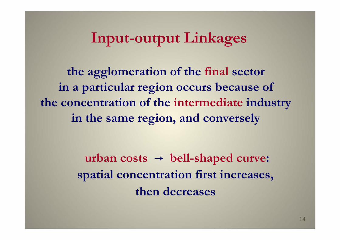
Input-output Linkages
the agglomeration of the final sector in a particular region occurs because of
the concentration of the intermediate industry in the same region, and conversely
urban costs → bell-shaped curve:spatial concentration first increases,
then decreases

15
Figure 2: Theil indices for the manufacturing sector
0
0,2
0,4
0,6
0,8
1860 1878 1895 1913 1930 1948 1965 1983 2000
Manu. Emp. Total Manu. Emp. Within Manu. Emp. Between

Figure 3: Theil indices for the service sector
0
0,2
0,4
0,6
0,8
1860 1878 1895 1913 1930 1948 1965 1983 2000
Ser. Emp. Total Ser. Emp. Within ser. Emp. Between
16

17
What Next?
(i) More general models(ii) Strategic considerations
(iii) The dimensionality problem
“the Heckscher-Ohlin theorem is derived from a model of only two of each of goods, countries, and factors of production. It is unclear what the theorem says should be true in the real world where there are many of all three” (Deardorff)

18
(iv) Local interactions → spatial scale
“density economies” :
log pl = α+ βlog den +ε
β ranges from 4 to 11%
endogeneity → simultaneity & omitted variables

19
even when we account for a large number of explanatory variables and
econometric issues, agglomeration economies remain important
β is about 3%
the elasticity of wages with respect to density is largely explained by
differences in workers’ skill

(v) Cities + development
20
(vi) Cities + trade + growth
(vii) Cities + trade + the supply chain

21
Thank you for your attention