patrons - cvr college of engineering
TRANSCRIPT


PATRONS
Dr. Raghava V. Cherabuddi, President & Chairman
Dr. K. Rama Sastri, Director
Dr. A. D. Raj Kumar, Principal
Editor : Dr. K. V. Chalapati Rao, Professor & Dean, Academics
Associate Editor : Wg. Cdr. Varghese Thattil, Professor, Dept. of ECE
Editorial Board :
Dr. K. Lal Kishore, Former Director, R&D and Registrar (Retd.), JNTUH.
Dr. S. Ramachandram, Vice Principal, College of Engineering &
Professor Dept. of CSE, Osmania University.
Prof. L. C. Siva Reddy, Vice Principal and Professor & Head, Dept. of CSE, CVRCE
Dr. M. S. Bhat, Professor & Dean, Evaluation, CVRCE
Dr. N. V. Rao, Professor, Dept. of CSE, CVRCE
Prof. R. Seetharamaiah, Professor & Head, Dept. of IT, CVRCE
Dr. K. Nayanathara, Professor & Head, Dept. of ECE, CVRCE
Dr. K. S. Dhanavanthri, Professor & Head, Dept. of EEE, CVRCE
Prof. S. Narayana, Professor & Head, Dept. of EIE, CVRCE
Dr. T. A. Janardhan Reddy, Professor & Head, Dept. of Mech. Engg., CVRCE
Dr. E. Narasimhacharyulu, Professor & Head, Dept. of H&S, CVRCE

CVR JOURNAL
OF
SCIENCE & TECHNOLOGY
CVR COLLEGE OF ENGINEERING (An Autonomous College affiliated to JNTU Hyderabad)
Mangalpalli(V), Ibrahimpatan(M),
R.R.District, A.P. – 501510
http://cvr.ac.in

EDITORIAL
The Second Volume of the CVR Journal of Science & Technology is being brought out
following the same guiding principles of maintaining relevance and excellence in the
contributions, as was indicated in the previous Volume. NATIONAL INSTITUTE OF
SCIENCE COMMUNICATION AND INFORMATION RESOURCES has registered the
Journal and assigned ISSN -2277-3916 based on the quality of contributions in Volume-1.
Accordingly the Volume-2 of our Journal includes the ISSN No. on cover page as well as on
each page of the Journal.
As was the case for the previous Volume of the Journal, we have received for the current
Volume, papers from all the Departments of the College. In addition we have received a few
contributions from outside the college. Following review by the Editorial Board, 19 papers have
been selected and included in the current Volume. The break-up of contributions from various
departments is: CSE-5, ECE-5, EEE-2, EIE-1, H & S-1, IT-2 and MBA-3.
Considering the importance of research culture among staff members in providing quality
education to students, it is gratifying to note that our staff members are pursuing active research
in addition to their teaching work as is evident from the quality of the papers. The present global
picture of technology demands constant updating of knowledge and skills of teachers if they
have to provide appropriate guidance to the students. With widespread use of Internet, there is no
dearth of information and the students have abundant opportunities to obtain latest knowledge in
any area. However they need guidance in appropriate utilization of the knowledge they acquire,
as per need in different contexts. It is for the teachers, with their maturity and experience, to
provide this kind of guidance. With the experience gained by contributing papers to Research
Journals, the teachers would acquire the requisite competence to provide valuable suggestions to
the students.
It is our earnest attempt to continue with the publication of the CVR Journal of Science
and Technology on a Bi-annual basis and make every attempt to constantly improve the quality
of our Journal. We hope thereby to contribute to the wider cause of serving Engineering
Education as per the needs of time.
K. V. CHALAPATI RAO

CONTENTS
CVR Journal of Science & Technology, Volume 2, June 2012 ISSN 2277-3916
Design Patterns For Scheduling Tasks In Real-Time Systems-----------------------------------------------------------------1
U V R Sarma, Dr K V Chalapati Rao, Dr P Premchand
Architecture Of Intelligent Process Controlling Model through Image Mining---------------------------------------------6
Dr Hari Ramakrishna
Pattern Methodology Of Documenting And Communicating Domain Specific Knowledge------------------------------9
Dr Hari Ramakrishna, Dr K V Chalapati Rao
Applying Principles Of LEAN In Academic Environments------------------------------------------------------------------16
S Suguna Mallika
Region-Wise Quality Measurements Of Pan-sharpened Images-------------------------------------------------------------19
G P Hegde, Dr I V Muralikrishna, Dr Nagaratna Hegde
Polarization Reconfigurable Microstrip Antennas For Wireless Communication-----------------------------------------27
A Bharathi, P Kavitha
Technology Scaling And Low Power Design Techniques--------------------------------------------------------------------30
T Esther Rani, Dr Rameshwar Rao, Dr M Asha Rani
Globalized Power Aware Routing Protocols For Mobile Ad Hoc Networks-----------------------------------------------40
Humaira Nishat, Dr D Srinivasa Rao
Survey On Android OS And C2DM Service------------------------------------------------------------------------------------43
R R Dhruva, V V N S Sudha
A Survey On Routing Protocols In Wireless Sensor Network----------------------------------------------------------------47
Shakeel Ahmed
Power Quality Improvement Using Interline Unified Power Quality Conditioner-----------------------------------------51
R N Bhargavi
Power System Transient Stability Analysis With SSSC Controller----------------------------------------------------------56
P Nagaraju Mandadi, Dr K Dhanvanthri
Control Of Process Variables For Remote Applications Using Lab VIEW and Internet----------------------------------61
S Harivardhagini, S Pranavanand
Numerical Solution Of Oscillatory Motion Of Dusty Memory Fluid Through Porous Media---------------------------67
D Sreenivas, B Shankar
Next Generation Network– A Study On QOS Mechanisms-------------------------------------------------------------------70
Dr B B Jayasingh, Sumitra Mallick
Extended AODV For Multi-Hop WMN------------------------------------------------------------------------------------------76
S Jyothsna
A Study On HR Practices In CVRCE--------------------------------------------------------------------------------------------80
Dr B Archana, Dr M S Bhat
Queuing Theory-A Tool For Optimizing Hospital Services------------------------------------------------------------------86
V R Girija, Dr M S Bhat
Effect of Inflation On Various Commodities------------------------------------------------------------------------------------90
Lalitha Suddapally

ISSN 2277 –3916 CVR Journal of Science & Technology, Volume 2, June 2012
Design Patterns For Scheduling Tasks In Real-
Time Systems U.V.R. Sarma
1, Dr. K. V. Chalapati Rao
2 and Dr. P. Premchand
3
1CVR College of Engineering, Department of CSE, Ibrahimpatan, R.R.District, A.P., India
Email: [email protected] 2CVR College of Engineering, Department of CSE, Ibrahimpatan, R.R.District, A.P., India
Email: [email protected] 3Osmania University, Department of CSE, Hyderabad, A.P., India
Email: [email protected]
Abstract—This paper discusses some of the popular design
patterns employed in scheduling tasks in various categories
of real-time applications and generalizes the guidelines for
designing and developing real-time systems. A tool is
proposed to automate the application of these patterns when
creating a detailed design model.
Index Terms—Design Pattern, Real-Time Systems, periodic,
aperiodic and sporadic tasks, EDF, SETF, LETF, Rate-
Monotonic Scheduling, Deadline-Monotonic Scheduling,
Priority Ceiling, Priority inversion, Least Laxity, Maximum
Urgency First.
I. INTRODUCTION
A design pattern is a generalized solution to a
commonly occurring problem [1]. It is not a finished
design that can be transformed directly into code – rather, it is a description or template, which helps in solving a
problem and can be used in many different situations.
Good OO designs are reusable, extensible and
maintainable. Patterns show us how to build systems
with good OO design qualities. Gamma and others,
popularly known as Gang of Four (GoF) list 23 design
patterns [1]. Usage of design patterns helps to lower
software costs.
A system is said to be real-time when
quantitative expressions of time are necessary to describe
the behavior of the system. Usually, there are many real-time tasks in such a system and are associated with some
time constraints. A real-time task is classified into either
hard, firm or soft real-time depending on the
consequences of a task failing to meet its timing
constraints. A real-time task is called hard if missing its
deadline may cause catastrophic consequences on the
environment under control. It is called firm if missing its
deadline makes the result useless, but missing does not
cause serious damage and it is called soft if meeting its
deadline is desirable (e.g. for performance reasons) but
missing does not cause serious damage.
Typical Hard RT activities include sensory data acquisition, detection of critical conditions and low-level
control of critical system components. Typical
application areas are power-train control, air-bag control,
steer by wire, brake by wire (automotive domain) and
engine control, aerodynamic control (aircraft domain).
Typical Firm RT Activities include decision support and
value prediction. Typical application areas are Weather
forecast, Decisions on stock exchange orders etc. Typical
Soft RT Activities include command interpreter of user
interface, keyboard handling, displaying messages on
screen, representing system state variables and
transmitting streaming data. Typical application areas are
communication systems (voice over IP), user interaction
and comfort electronics (body electronics in cars).
Appropriate scheduling of tasks is the basic
mechanism adopted by a real-time operating system to meet the constraints of a task. Therefore, selection of an
appropriate task scheduling algorithm is central to the
proper functioning of a real-time system.
II. TYPES OF REAL-TIME TASKS
A task is an executable entity of work, characterized
by task execution properties, task release constraints, task
completion constraints and task dependencies. Tasks are
executed in a system made up of a processor (CPU) and
other resources (communication links, shared data etc.)
Task execution properties include Worst-case
execution time, Criticality level, Preemptive / non-preemptive execution and whether a task can be
suspended or not during execution.
Based on the way real-time tasks recur over a period of
time, it is possible to classify them into three main
categories: periodic, aperiodic and sporadic tasks.
A periodic task is one that repeats after a certain fixed
time interval. Deadlines have to be met with precision,
and so they are hard real-time in nature, whereas an
aperiodic task can arise at random instants but we can
afford to miss few deadlines and hence soft real-time in
nature. A sporadic task is one that recurs at random
instants and mostly hard real-time in nature.
III. SCHEDULING APPROACHES
Three commonly used approaches to scheduling Real-
Time Systems are [2]:
1. Clock-Driven approach.
2. Round-Robin approach
3. Priority-Driven approach.
3.1 Clock-Driven approach (also called time-driven)
In this approach, decisions on task execution are
made at specific time instants. All the parameters of the
CVR College of Engineering 1

ISSN 2277 –3916 CVR Journal of Science & Technology, Volume 2, June 2012
tasks are fixed and known apriority. Schedules are
computed off-line and stored for use at run-time. Hence
scheduler overhead during run-time is minimized. H/W
timer is used to regularly space time instants. Scheduler
selects the task, blocks, and after expiry of timer, awakes
and repeats these actions.
3.2 Round-Robin approach
This approach follows the fairness principle – justice
to all. It is commonly used for scheduling time-shared
applications (time slice – in the order of tens of msec). A
FIFO queue of tasks ready for execution is maintained.
An executing task is preempted at the end of time slice.
1/nth share for n tasks in a round (hence called processor-
sharing algorithm). A variation to this approach is
weighted round robin. Different tasks may have different
weights – for ex., a task with weight wt gets wt time slices every round; the length of the round is equal to the
sum of the weights of all the ready tasks; weights can be
adjusted to speed up / retard the progress of each task.
Round Robin approach is not suitable for tasks
requiring good response time, particularly when we have
precedence constrained tasks, but suitable for incremental
consumption – for ex., UNIX pipe. In case of pipelining,
they can complete even earlier – ex: Transmission of
messages by switches en route in a pipeline fashion. The
approach does not require a sorted priority queue; it uses
only a round-robin queue; which is a distinct advantage,
since priority queues are expensive.
3.3 Priority-Driven approach
These algorithms never leave any resource idle
intentionally. Scheduling decisions are made when
events such as releases and completion of tasks occur;
hence called event-driven. Other names – greedy scheduling, list scheduling and work-conserving
scheduling.
Most scheduling algorithms used in non-real-time
systems are priority-driven. Examples include FIFO,
LIFO – priorities based on release times; SETF (Shortest-
Execution-Time-First) and LETF (Longest-Execution-
Time-First) – priorities based on execution times.
Priority-driven algorithms can be implemented with
either preemptive or non-preemptive scheduling. In some
cases, non-preemptive scheduling may look attractive,
but, in general, non-preemptive scheduling is not better
than preemptive scheduling. Priority-based scheduling systems operate in one of
three primary modes:
1. Static priority systems,
2. Semi-static or
3. Dynamic priority systems.
3.3.1 Static Priority System: In a static system, a task’s
priority is determined at compile time and is not changed
during execution. This has the advantages of simplicity of
implementation and simplicity of analysis. The most
common way of selecting task priority is based on the
period of the task, or, for asynchronous event-driven tasks, the minimum arrival time between initiating events.
This is called Rate Monotonic Scheduling (RMS). Static
scheduling systems may be analyzed for schedulability
using mathematical techniques such as Rate Monotonic
Analysis.
Another well-known fixed priority algorithm is the
Deadline-Monotonic (DM) algorithm. This algorithm
assigns priorities to tasks according to their relative
deadlines: the shorter the relative deadline, the higher the
priority. Clearly, when the relative deadline of every task
is proportional to its period, the RMS and DM algorithms
are identical. When the relative deadlines are arbitrary,
the DM algorithm performs better in the sense that it can
sometimes produce a flexible schedule when the RMS algorithm fails, while the RMS algorithm always fails
when the DM algorithm fails.
3.3.2 Semi-Static Priority System: Semi-static priority
systems assign a task a nominal priority but adjust the
priority based on the desire to limit priority inversion.
This is the essence of the priority ceiling pattern. If a low
priority task locks a resource needed by a high priority
task, the high priority task must block itself and allow the
low priority task to execute, at least long enough to
release the needed resource. The execution of a low
priority task when a higher priority task is ready to run is called priority inversion. The naïve implementation of
semaphores and monitors allows the low priority task to
be interrupted by higher priority tasks that do not need
the resource. Because this preemption can occur
arbitrarily deep, the priority inversion is said to be
unbounded. It is impossible to avoid at least one level of
priority inversion in multitasking systems that must share
resources, but one would like to at least bound the level
of inversion. This problem is addressed by the priority
ceiling pattern. The basic idea of the priority ceiling
pattern is that each resource has an attribute called its priority ceiling. The value of this attribute is the highest
priority of any task that could ever use that particular
resource. The active objects have two related attributes:
nominal priority and current priority. The nominal
priority is the normal executing priority of the task. The
object’s current priority is changed to the priority ceiling
of a resource it has currently locked as long as the latter is
higher.
3.3.3 Dynamic Priority System: Dynamic priority
systems assign task priority at run-time based on one of
several possible strategies. The three most common
dynamic priority strategies are: 1. Earliest Deadline First
2. Least Laxity
3. Maximum Urgency First
In Earliest Deadline First (EDF) scheduling, tasks are
selected for execution based on which has the closest
deadline. This algorithm is said to be dynamic because
task scheduling cannot be determined at design time, but
only when the system runs. In this algorithm, a set of
tasks is schedulable if the sum of the task loadings is less
than 100%. This algorithm is optimal in the sense that if
it is schedulable by other algorithms, then it is also schedulable by EDF. However, EDF is not stable; if the
total task load rises above 100%, then at least one task
will miss its deadline, and it is not possible to predict in
general which task will fail. This algorithm requires
2 CVR College of Engineering

ISSN 2277 –3916 CVR Journal of Science & Technology, Volume 2, June 2012
additional run-time overhead because the scheduler must
check all waiting tasks for their next deadline frequently.
In addition, there are no formal methods to prove
schedulability before the system is implemented.
Laxity for a task is defined as the time to deadline
minus the task execution time remaining. Clearly, a task
with a negative laxity has already missed its deadline.
The algorithm schedules tasks in ascending order of their
laxity. The difficulty is that during run-time, the system
must know expected execution time and also track total
time a task has been executing in order to compute its laxity. While this is not conceptually difficult, it means
that designers and implementers must identify the
deadlines and execution times for the tasks and update the
information for the scheduler every time they modify the
system. In a system with hard and soft deadlines, the
Least Laxity (LL) algorithm must be merged with another
so that hard deadlines can be met at the expense of tasks
that must meet average response time requirements (see
MUF, below). LL has the same disadvantages as the EDF
algorithm: it is not stable; it adds run-time overhead over
what is required for static scheduling, and schedulability of tasks cannot be proven formally.
Maximum Urgency First (MUF) scheduling is a hybrid
of RMS and LL. Tasks are initially ordered by period, as
in RMS. An additional binary task parameter, criticality,
is added. The first n tasks of high criticality that load
under 100% become the critical task set. It is this set to
which the Least Laxity Scheduling is applied. Only if no
critical tasks are waiting to run are tasks from the
noncritical task set scheduled. Because MUF has a
critical set based on RMS, it can be structured so that no
critical tasks will fail to meet their deadlines.
IV. PATTERNS
With this background of various scheduling
approaches in Real-Time Systems, we can now suggest
suitable patterns known as Execution Control Patterns for
scheduling tasks. They deal with the policy by which
tasks are executed in a multitasking system. This is
normally executed by the Real-Time Operating System, if
present. Most Real-Time Operating Systems offer a
variety of scheduling options. The most important of
these are listed here as execution control patterns [3].
1. Cyclic Executive Pattern for simple task
scheduling. 2. Time Slicing – Round Robin Pattern –
fairness in task scheduling.
3. Static Priority Pattern – preemptive
multitasking for schedulable systems.
4. Semi-static priority – Priority Ceiling
Pattern.
5. Dynamic Priority Pattern – preemptive
multitasking for complex systems.
The primary difference occurs in the policy used for
the selection of the currently executing task.
4.1 Cyclic Executive Pattern
In the cyclic executive pattern the kernel (commonly
called the executive in this case) executes the tasks in a
prescribed sequence. Cyclic executives have the
advantage that they are “brain-dead” simple to implement
and are particularly effective for simple repetitive tasking
problems. Also, it can be written to run in highly
memory-constrained systems where a full RTOS may not
be an option. However, they are not efficient for systems
that must react to asynchronous events and not optimal in
their use of time. There have been well-publicized cases
of systems that could not be scheduled with a cyclic
executive but were successfully scheduled using
preemptive scheduling. Another disadvantage of the cyclic executive pattern is that any change in the
executive time of any task usually requires a substantial
tuning effort to optimize the timeliness of responses.
Furthermore, if the system slips its schedule, there is no
guarantee or control over which task will miss its
deadline preferentially.
Figure 1.[4] shows how simple this pattern is. The set
of threads is maintained as an ordered list (indicated by
the constraint on the association end attached to the
Abstract Thread class). The Cyclic Executive merely
executes the threads in turn and then restarts at the beginning when done. When the Scheduler starts, it must
instantiate all the tasks before cycling through them.
Figure 1.Cyclic Executive Pattern
4.2 Time Slicing – Round Robin Pattern
The kernel in the time slicing pattern executes each
task in a round-robin fashion, giving each task a specific
period of time in which to run. When the task’s time
budget for the cycle is exhausted, the task is preempted
and the next task in the queue is started. Time slicing has
the same advantages of the cyclic executive but is more
time based. Thus it becomes simpler to ensure that
periodic tasks are handled in a timely fashion. However, this pattern also suffers from similar problems as the
cyclic executive. Additionally, the time slicing pattern
doesn’t “scale up” to large numbers of tasks well because
the slice for each task becomes proportionally smaller as
tasks are added.
The Round Robin Pattern is a simple variation of the
Cyclic Executive Pattern. The difference is that the
Scheduler has the ability to preempt running tasks and
CVR College of Engineering 3

ISSN 2277 –3916 CVR Journal of Science & Technology, Volume 2, June 2012
does so when it receives a tick message from its
associated Timer. Two forms of the Round Robin Pattern
are shown below. The complete form (Figure 2a [4])
shows the infrastructure classes Task Control Block and
Stack. The simplified form (Figure 2b [4]) omits these
classes.
Figure 2. Round Robin Pattern
4.3 Static Priority Pattern
In a static system, a task’s priority is determined at
compile time and is not changed during execution. This has the advantages of simplicity of implementation and
simplicity of analysis.
Figure 3. [4] shows the basic structure of the pattern.
Each «active» object (called Concrete Thread in the
figure) registers with the Scheduler object in the
operating system by calling createThread operation and
passing to it, the address of a method defined. Each
Concrete Thread executes until it completes (which it
signals to the OS by calling Scheduler::return()), it is
preempted by a higher-priority task being inserted into
the Ready Queue, or it is blocked in an attempt to access
a Shared Resource that has a locked Mutex semaphore.
Figure 3. Static Priority Pattern
4.4 Semi-static Priority - Priority Ceiling Pattern
The Priority Ceiling Pattern, or Priority Ceiling
Protocol (PCP) as it is sometimes called, addresses both
issues of bounding priority inversion (and hence
bounding blocking time) and removal of deadlock. It is a
relatively sophisticated approach, more complex than the
previous methods. It is not as widely supported by
commercial RTOSs, however, and so its implementation
often requires writing extensions to the RTOS. Figure 4.
[4] shows the Priority Ceiling Pattern structure.
Figure 4. Priority Ceiling Pattern
4.5 Dynamic Priority Pattern
The Dynamic Priority Pattern is similar to the Static
Priority Pattern except that the former automatically
updates the priority of tasks as they run to reflect
changing conditions. There are a large number of possible
strategies to change the task priority dynamically. The
most common is called Earliest Deadline First, in which
4 CVR College of Engineering

ISSN 2277 –3916 CVR Journal of Science & Technology, Volume 2, June 2012
the highest-priority task is the one with the nearest
deadline. The Dynamic Priority Pattern explicitly
emphasizes urgency over criticality.
Figure 5.[4] shows the Dynamic Priority pattern
structure.
Figure 5. Dynamic Priority Pattern
V. TOOL SUPPORT
It is proposed to develop a GUI based tool, which will
help the users in selecting appropriate scheduling strategy
depending upon the nature and parameters of the real-
time tasks in the application being developed. The tool will educate the users about merits and demerits of each
scheduling strategy and help in identifying appropriate
design pattern. Further, the tool will also generate the
code for the chosen design pattern in real-time java.
Thus, the design and development activities may be
completed in less time and with more accuracy, as the
code is generated automatically.
CONCLUSIONS
In this paper, we have reviewed and summarized
various scheduling approaches for real-time systems.
Further, we have listed suitable design patterns for these
varied scheduling strategies. The proposed tool to generate code for a chosen design pattern will greatly
help the developer in reducing development effort,
reducing development time and provides ready-made
code, which can be plugged into the developer’s
application.
REFERENCES
[1] Gamma, Erich, Richard Helm, Ralph Johnson, and John Vlissides. Design Patterns: Elements of Reusable Object-Oriented Software. Reading, MA: Addison-Wesley, 1995.
[2] Jane W.S. Liu, Real-Time Systems, Pearson Education 2006.
[3] Bruce Powel Douglass, White Paper on Real-Time Design Patterns 1998
[4] Bruce Powel Douglass Real-Time Design Patterns: Robust Scalable Architecture for Real-Time Systems, Addison Wesley 2002
[5] Stankovic, J., M. Spuri, K. Ramamritham, and G. Buttazzo. Deadline Scheduling for Real-Time Systems, Norwell, MA: Kluwer Academic Press, 1998.
[6] Douglass, Bruce Powel. Doing Hard Time: Developing Real-Time Systems with UML, Objects, Frameworks, and
Patterns, Reading, MA: Addison-Wesley, 1999. [7] A System of Patterns: Pattern-Oriented Software
Architecture Buschmann, et. al., John Wiley & Sons, 1996.
CVR College of Engineering 5

ISSN 2277 –3916 CVR Journal of Science & Technology, Volume 2, June 2012
Architecture Of Intelligent Process Controlling
Model Through Image Mining Dr.Hari Ramakrishna
Chaitanya Bharathi Institute of Technology, Department of CSE, Hyderabad, A.P., India
Email: [email protected]
Abstract—In this paper, research potentials and challenges
raised through visual data mining and image mining are
presented. Various views of visual data mining and a new
vision of visual data mining and its applications are
discussed. A case study of an application of visual data and
image mining for improving quality processes of an
educational organization is presented. Various research
challenges raised by such image mining applications are
described.
Index Terms— Knowledge acquisition, Visual Data mining,
Data Mining, Image Mining, Real time data mining,
Architectural framework, Process Controller.
I. INTRODUCTION
An image is equal to thousands of words. It is possible
to present complex data in a predefined format of an
image. For Example, Software engineering domain uses
UML which represents its models in the form of a set of
diagrams. These UML diagrams has particular schema
and defines a set of rules for designing. These UML Models holds lot of information with semantic meaning.
A software developer can get required information along
with complex logic of system from these UML diagrams.
Similarly, most of the images represent lot of data
without following a particular pattern or rule. Extracting
information and patterns from the data available in an
image or a set of images can be referred as Image mining.
A satellite Image holds lot of information in an
unprocessed form. Many researchers are using Data
Mining Algorithms for extract information and
knowledge from satellite images [4].
A Human Expert gains knowledge from the images
captured through his vision applying natural data mining
algorithms running in his mind known as human
intelligence. This enables a human expert to control set
of quality processes of any domain of his expertise. A
robot can mimic exactly like a human expert if it is
charged with powerful Image mining algorithms through
an intelligent software framework.
This paper presents model application framework
using Visual Data mining and image mining for
improving quality of processes of an organization through visual aids and intelligent software model. A case study
of controlling educational processes through visual data
and image mining is discussed in this paper.
II. VISUAL DATA MINING VS VISUAL DATA
The term Visual Data mining is defined differently
depending on its usage at deferent application. The Data
Mining defined visual data mining as a tool to represent
graphical data for taking decisions. It is used to represent
complex data sets or patterns in a graphical form for
taking decisions. Though it proves that a graph or an
image can be used to generate knowledge from complex
data sets, it is limiting the word only to the extent of
generating set of mathematical graphs. This paper uses
the word for extracting information and knowledge from real time images generated through visual aids for taking
decisions.
Visual data plays a major role in knowledge extraction.
Educational experts suggest visual tools (Visual Aids) as
better process for knowledge acquisition and better
communication even for a human expert. The word
Visual data mining should be redefined for better use as
set of algorithms models which extract data from images
collected using visual aids for acquiring required
knowledge for taking decisions. The term visual aid refers
to human eye, a Video or digital Camera or a satellite. A
human Expert extracts Knowledge for taking decisions through his sight applying natural Visual data and image
mining algorithms functioning in this mind.
Applying such concepts enables a computer based
system to take decisions through extracting knowledge
from images collected from digital device. The final
objective of such models is to charge the robots with
powerful knowledge acquisition algorithms to mimic like
a human expert collecting data from visual devices
(multimedia devices).
III. A CASE STUDY OF INTELLIGENT PROCESS
CONTROLLER EDUCATIONAL ORGANIZATION
A. E-College System
The E-college Product is a Web based Software Model
which automates the processes of a huge educational
organization. General objective of any educational
environment is to control the educational processes to
produce the best professionals to the society. Several
methodologies are available to improve the educational
process with the help of Information Technology. E-
College is a Computer based system which implements
processes of a Huge Educational organization for improving the quality of the educational system.
6 CVR College of Engineering

ISSN 2277 –3916 CVR Journal of Science & Technology, Volume 2, June 2012
B. Architectural of intelligent process control model for
ECollege
The major challenge of educational process is to
monitor the academic processes. For example consider
the process of monitoring the attendance of the students in the class rooms. This will be managed with attendance
registers. All the registers data can be made available
over internet either adding the data from the registers or
by automatically collecting from finger-prints of the
students from the class rooms. This will not provide
authenticated information for the following questions:
1. Whether all students are present throughout the
class?
2. When the class started? What will be the
strength of the class at the beginning and at the
end? 3. Any malpractice took place in giving the
attendance?
The solutions for all the questions will be by
appointing an agent or an academic controller who will
be observing the classes on line. This can be done even
by keeping the digital cameras in the class and observing
them. Such process has the following disadvantages:
1. The data is not persisted?
2. Very difficult for a human controller to monitor
if the number of classes are large and the class
schedules (or time tables) are complex.
The solutions for such processes are addressed by a simple intelligent software model. This model controls
the classes with the visual aids. The computer module can
manage complex class schedules and huge data. In the
computer modules can collect visual pictures from
required classes and extract data and make them
persistent. This enable the module to evaluate the
regularity of the class room lectures.
This model is replacing a Dean Academics who
monitors the class rooms functioning with Software
Module capable of collecting real time data from the class
rooms using simple digital cameras and a software model.
IV. CLASS ROOM MONITOR ARCHITECTURE
Architecture of the Class Room Monitor is presented in
the following Figure 1.
In this model class rooms are equipped with digital
cameras. The class room database consists of information
related to class room sessions. The visual data collector
will collect the information in visual form with the help
of digital cameras based on class room schedule
databases. This will extract required information from
visual data and builds suitable data base with collected
visuals. Typical data mining algorithms are applied for
building Knowledgebase. The knowledge base is used to extract required information for decision making.
Such systems can be used to measure regularity of the
class room lectures, regularity of students attending the
class and regularity of the faculty. This system works like
an automated real time software dean academics for
monitoring the class room lectures. Similar models can
be developed for several such applications for monitoring
the processes of organizations for improving the
performance.
Picture are collected depending on class schedules and
prescribed frequencies. For example if a class start at 9am
and duration is one hour we can set system such that it collect pictures at 9.00 9.15 and 9.30 and 945 and 10.00
and 10.15. This will enable expert providing the
following answers.
1. When the class started? How many students at
the beginning of the class?
2. When all students are present in class?
3. When the class ended? How many students are
present at the end of class?
4. Whether the class ended at time or not?
Digital devices can be configures to take pictures
depending on time or on events as per the need of the system. This logic can be extended to other multimedia
devices such as audio or video devices.
Such systems need software facilities to update
changes in the timetables at run time which enable to
change the class room or to change teacher, in order to
make the visual devices act accordingly.
V. IMAGE MINING REQUIREMENTS
This model identifies and raises requirements from
image mining which enforse the human expert to
interfear for automatic decition making. In this model a
human expert is neded to identify the number of students
in the class room from the picture collected and stored in database. Image mining algorithom which collect
number of students in a class from the picture makes the
software model totally automated. An alogorithm to
Figure: 1 Class Room Monitor
Figure 1: Architecture of Classroom monitoring system
Visual Data
Base
Class Rooms with Digital Cameras
Knowledge
Base
Decision Making System
Data mining Tool
Visual Data
Collector
Class Room
Database
CVR College of Engineering 7

ISSN 2277 –3916 CVR Journal of Science & Technology, Volume 2, June 2012
recorgnize a student from a picture with total confidence
will enable the software to generate automated attendence
register with a simple picture collected.[1,2,3,5,7]
V. OTHER APPLICATIONS
We can find several applications which are useful for
rural development. Farmers who involve in cultivation
need advice on their crops at frequent intervals of time.
Similar software model which collects images as per the
requirement can be used for advising the farmers. Like
medical image mining algorithms which recognize
medical problems if algorithms are generated for finding problems from villages can be benefited through these
models. [8] At present similar software models are
available but not fully automated. Fully automated
models decrease human expert time and provide fast
decisions which are required for providing immediate
solutions for the problem. This will enable to use such
applications even for Disaster Management.
Several similar applications based on image mining are
in use. For example Traffic Control system of several
contrives take pictures of vehicles which violate the
traffic rule. They have the intelligence of recognizing the number automatically from the picture and collect the
details of the owner and vehicle from online database.
Such systems have the capability of automatically
recording the defaulters. [6]
Similar other application is for the payment of the bills
from the scanned hard copy of the bill. The image mining
algorithm can recognize the validity of the bill along with
bill number, customer details and amount payment
details. The percentage of the accuracy of the information
collected from these image mining algorithms changes
with risk rate of the applications.
CONCLUSIONS
This paper identifies the need to develop the intelligent
software models for improving the organizational
processes through data mining techniques. It also
indentifies the need in the domain of image mining which
supports such processes for total automation. The paper
identified the use of the multimedia devices and data
mining algorithms to extract information through them to
enable software models to mimic like human experts
through total automation of the software. This paper
identified the need for redefining the visual data mining
from „providing visual tools to human expert for taking decisions‟ to “extracting information from visuals” for
total automation.
ACKNOWLEDGMENT
The authors wish to thank faculty of computer science
and engineering department of CBIT who are doing
research in Image processing and data mining for their
suggestions and for participating in the discussions.
REFERENCES
[1] G. Kukharev and E. Kamenskaya, “Application of two-dimensional canonical correlation analysis for
face image processing and recognition” , Pattern Recognition and Image Analysis ,Volume 20, Number 2 june 2010.
[2] N. ALUGUPALLY, A. SAMAL, D. MARX AND S. BHATIA, “ANALYSIS OF LANDMARKS IN RECOGNITION OF FACE
EXPRESSIONS “Pattern Recognition and Image Analysis ,Volume 21, Number 4 December 2011.
[3] Araujo A., Bellon O., Silva L., Vieira E., Cat M.
"Applying Image Mining to Support Gestational Age Determination" The Insight Journal, June 30, 2006, presented at MICCAI Open Science Workshop.
[4] "An Useful Information Extraction using Image Mining Techniques from Remotely Sensed Image" Dr.C.Jothi Venkateswaran et al. / (IJCSE) International Journal on Computer Science and Engineering Vol. 02, No. 08, 2010, 2577-2580.
[5] Hilliges O., Kunath P., Pryakhin A., Butz A., Kriegel
H.-P.: "Browsing and Sorting Digital Pictures using Automatic Image Classification and Quality Analysis", Proc. 12th Int. Conf. on Human-Computer Interaction (HCII'07), Beijing, China, 2007, in: LNCS, Vol. 4552, 2007, pp. 882-891.
[6] Kriegel H.-P., Kunath P., Pfeifle M., Renz M.: ViEWNet: “Visual Exploration of Region-Wide Traffic Networks”, Proc. 22nd Int. Conf. on Data
Engineering (ICDE 2006), Atlanta, GA, 2006, paper no. 166.
[7] Multimedia Data Mining (MDM/KDD'03), Washington, DC, 2003, pp. 64-71.
[8] “E-Sagu: An IT based Personalized Agro-Advisory System “A Project of Media Lab AsiaExecuted by IIIT, Hyderabad and Media Lab Asia in association with Nokia, http://www.esagu.in.
8 CVR College of Engineering

ISSN 2277 –3916 CVR Journal of Science & Technology, Volume 2, June 2012
Pattern Methodology Of Documenting And
Communicating Domain Specific Knowledge Dr.Hari Ramakrishna
1 and Dr.K.V Chalapathi Rao
2
1Chaitanya Bharathi Institute of Technology, Department of CSE, Hyderabad, A.P., India
Email: [email protected] 2CVR College of Engineering, Department of CSE, Ibrahimpatan, R.R.District, A.P., India
Email: [email protected]
Abstract— the main objective of this paper is to present
pattern methodology of documenting and communicating
domain specific knowledge along with a brief historic review
of the domain. This paper presents pattern methodology of
documenting domain specific knowledge along with few
simple framework samples.
Index Terms—pattern, pattern language, frameworks,
pattern frames, Graphic frameworks.
I. INTRODUCTION
Patterns for software development are one of the latest trends to emerge from the object oriented approach.
Fundamental to any science or engineering discipline is a
common vocabulary for expressing its concepts, and a
language for expressing these interrelationships. The goal
of patterns within the software community is to create a
body of literature to help software developers resolve
recurring problems encountered throughout all of
software development. Patterns help create a shared
language for communicating insight and experience about
these problems and their solutions.
The current use of the term pattern is derived from the writings of the architect Christopher Alexander who has
written several books on the topic as it relates to urban
planning and building architecture. Although these books
are ostensibly about architecture and urban planning, they
are applicable to many other disciplines, including
software development.
Alexander proposes a paradigm for architecture based
on three concepts namely Quality, Gate and the Way.
Quality is freedom, wholeness, completeness, comfort,
harmony, habitability, durability, openness, resilience,
variability and adaptability. The gate is the mechanism
that allows us to reach the quality. And the Way is progressively evolving an initial architecture, which then
flourishes into a live design possessing the quality. [1]
In 1987 Ward Cunningham and Kent Beck were
working with Smalltalk and designed user interfaces.
They decided to use some of Alexander‟s ideas to
develop a small five-pattern language for guiding novice
Smalltalk programmers. They presented the results at
OOPSLA-87 in Orlando in the paper “Using Patterns
Language for Object-Oriented Programming”. Soon
after, Jim Coplien (referred to as Cope) began compiling
a catalog of C++ idioms. These are one kind of patterns. Later they are published as “Advanced C++
Programming Styles and Idioms”. [2]
From 1990 to 1992 the members of GOF (Erich Gamma, Richard Helm, Ralph Johnson and John
Glissades frequently referred as GOF Gang of Four) had
done some work compiling a catalog of patterns.
Discussions of patterns abounded at OOPSLA-91
workshop conducted by Bruce Andersen. This was
repeated in 1992. Many pattern domain experts
participated in these workshops including Jim Coplien,
Doug Lea, Desmond D’Souza,Norm Kerth, Wolfgang
Pree and others.
In August 1993, Kent Beck and Grady Booch
sponsored a mountain retreat in Colorado, the first meeting of what is now known as the Hillside Group.
Another pattern workshop was held at OOPSLA –93 and
then in April of 1994, the Hillside Group met again to
plan the first conference on Patterns Languages for
Program Design (referred as PloP or PloPD). Shortly
thereafter the GOF released a book on Design Patterns
[3]. Most of the patterns presented in that book are from
Erich‟s Ph.D thesis. Several conferences are continuously
organized on this domain.
Software patterns first became popular with the wide
acceptance of the book „Design Patterns: Elements of
Reusable Object-Oriented Software’. Patterns have been used for many different domains ranging from
organizations and processes to teaching and architecture.
At present the software community is using patterns
largely for software architecture, design, development
processes and organizations. Though several conference
proceedings and books are available on this domain ,
other books that helped popularize patterns are „Pattern-
Oriented Software Architecture: A system of Patterns „
(also called as POSA book) by Frank Buschmann, Regine
Meunier, Hans Rohnert, Peter Sommerlad, and Michael
Stal ( referred as Gang of Five GoV ). Collection of selected papers from the first and second conferences on
Patterns Languages for Program Design is released as a
book namely “Pattern Languages of Program Design”.
At present Patterns are adopted into application
domains for example: [4].
i) Patterns in software development generally,
including software design, software engineering,
and software architecture
ii) Process patterns for management and
development processes
iii) Patterns for human-computer interaction (user-
interface patterns, or novel modes of interaction)
CVR College of Engineering 9

ISSN 2277 –3916 CVR Journal of Science & Technology, Volume 2, June 2012
iv) Patterns for education (ranging from
professional training to classroom teaching)
v) Patterns for business and organizations
vi) Modeling patterns, analysis patterns, design
patterns
vii) Patterns for object-oriented design, aspect-
oriented design, and software design generally
viii) Patterns to describe libraries, frameworks, and
other reusable software elements
ix) Patterns for middleware, including distribution,
optimization, security, and performance improvement
x) Domain specific patterns and technology
specific patterns, as well as generic patterns
xi) Patterns for refactoring and reengineering
xii) Formal models and type systems for patterns
xiii) Programming environments, software
repositories, and programming languages for
patterns
xiv) The use of patterns to improve quality attributes
such as adaptability, evolvability, reusability and
cost-effectiveness
II. PATTERNS AND PATTERN LANGUAGES
Pattern can be defined as “Reusable solution for
recurring problem”. Patterns Dirk Riehle and Heinz
Zullighoven define pattern as, “the Abstraction from a
concrete form, which keeps recurring in specific non-
arbitrary contexts”. Another definition of pattern for
software community is given as, “a named nugget of
insight that conveys the essence of a proven solution to a
recurring problem within a certain context amidst
competing concerns”.
Each pattern is a three-part rule, which expresses a relation between a certain context, and a certain system of
forces, which occurs repeatedly in that context, and a
certain software configuration, which allows these forces
to resolve themselves. Alexander defines three-part
rule, as “Each pattern is a three-part rule, which
expresses a relation between a certain context, a problem
and a solution.”
Cope says that a good pattern does the following:
1) It solves a Problem
2) It is a proven concept
3) The solution is not obvious
4) It describes a relationship 5) The pattern has a significant human component
(like comfort, quality of life)
If something is not a pattern, it doesn‟t mean that it is
not good. Similarly if it is a pattern, hopefully it is good
but need not be always. Many of the initial patterns
focused in the software community are design patterns.
The patterns in the GOF book are Object Oriented Design
Patterns [3]. There are many other kinds of software
patterns beside design patterns, analysis patterns
published by Marin Fowler and other patterns like
organizational patterns are also available. Architectural patterns express a fundamental structural
organization or schema for software systems. Design
Patterns provide a schema for refining the subsystems or
components of a software system or the relationships
between them. They describe commonly recurring
structure of communicating components that solve a
general design problem within a particular context.
Idioms are low-level patterns specific to a
programming language. An idiom describes how to
implement particular aspects of component or the
relationship between them using the features of the given
language. The difference between these patterns is in
their corresponding level of abstraction.
Riehle and Zullighoven have classified patterns as Conceptual patterns, Design Patterns and Programming
Patterns [12].
A collection of patterns forms a vocabulary for
understanding and communicating ideas. A pattern
language is such collection skillfully woven together into
a cohesive “whole” that reveals the inherent structure and
relationships of its constituent parts towards fulfilling a
shared objective [1]. If a pattern is a recurring solution to
a problem in a context given by some forces, then a
pattern language is a collection of such solutions, which
at every level of scale, work together to resolve a complex problem into an orderly solution according to a
predefined goal.
Cope defines a pattern language as a collection of
patterns and the rules to combine them into an
architectural style. Pattern languages describe software
frameworks or families of related systems [5, 6, and 7]. In
some other context, Cope defines pattern language as a
structured collection of patterns that build on each other
to transform needs and constraints into architecture.
III. DOMAIN SPECIFIC PATTERN LANGUAGES
The following is a description of view on domain specific patterns and pattern languages as per the domain
experts.
The domain-specific patterns are confidential –they
represent a company‟s knowledge and expertise about
how to build particular kinds of applications; so
references to them are not generally available. One can
however more and more of this knowledge will become
public over time. In the long run, sharing experience is
usually more effective for everyone than trying to hold
onto secrets.
The development of complete pattern language is an
optimistic but worthwhile goal. Such a language provides solutions to all design problems that can occur in the
respective domains. Christopher Alexander claims to
have done this in the domain of Architecture. Pattern
language already exists for small sub-domains of
software design, for example the CHECKS pattern
language for information integrity [8].
It would be very beneficial to have a pattern language
that covers a substantial part of the design space of the
respective domains.
IV. FRAMEWORKS
The software frameworks are closely related to design patterns and object-orientation. A software framework is
10 CVR College of Engineering
ISSN 2277 –3916 CVR Journal of Science & Technology, Volume 2, June 2012
a reusable mini-architecture that provides the generic
structure and behavior for a family of software
abstractions, along with a context of mimes/metaphors
that specify their collaboration and use within a given
domain. The following presents views of Brad Appleton
on frameworks.
The framework accomplishes patterns by hard coding
the context into a kind of "virtual machine" (or "virtual
engine"), while making the abstractions open-ended by
designing them with specific plug-points (also called hot
spots). These plug-points (typically implemented using callbacks, polymorphism, or delegation) enable the
framework to be adapted and extended to fit varying
needs, and to be successfully combined with other
frameworks. A framework is usually not a complete
application: it often lacks the necessary application-
specific functionality. Instead, an application may be
constructed from one or more frameworks by inserting
this missing functionality into the plug-and-play "outlets"
provided by the frameworks. Thus, a framework supplies
the infrastructure and mechanisms that execute a policy
for interaction between abstract components with open implementations [9].
The GOF also defines object-oriented frameworks as:
“a set of cooperating classes that makeup a reusable
design for a specific class of software”. A framework
provides architectural guidance by partitioning the design
into abstract classes and defining their responsibilities
and collaborations. A developer customizes a framework
to a particular application by sub classing and composing
instances of framework classes. For example Microsoft
Application framework belongs to this kind.
A framework dictates the architecture of the application. It will define the overall structure, such as
partitioning into classes and objects, the key
responsibilities, how the classes and objects collaborate,
and the thread of control
A framework predefines these design parameters so
that the application designer/implementer can concentrate
on the specifics of the application. The framework
captures the design decisions that are common to its
application domain. Frameworks thus emphasize design
reuse rather than code reuse, though a framework will
usually includes concrete subclasses that work directly.
The difference between a framework and an ordinary programming library is that a framework employs an
inverted flow of control between itself and its clients.
When using a framework, one usually just implements a
few callback functions, or a few specialized classes, and
then invokes a single method or procedure. At this point,
the framework does the rest of the work, invoking any
necessary client callbacks or methods at the appropriate
time and place. For this reason, frameworks are often said
to abide by the Hollywood Principle "Don't call us, we'll
call you." or the Greyhound Principle "Leave the driving
to us.” Design patterns may be employed both in the design
and the documentation of a framework. A single
framework typically encompasses several design patterns.
In fact, a framework can be viewed as the implementation
of a system of design patterns. Despite the fact that they
are related in this manner, it is important to recognize that
frameworks and design patterns are two distinctly
separate entities: a framework is executable software,
whereas design patterns represent knowledge and
experience about software. In this respect, frameworks
are of a physical nature, while patterns are of a logical
nature: frameworks are the physical realization of one or
more software pattern solutions; patterns are the
instructions for how to implement those solutions.
The major differences between design patterns and frameworks are as follows: [3].
Design patterns are more abstract than frameworks.
Frameworks can be embodied in code, but only examples
of patterns can be embodied in code. Strength of
frameworks is that they can be written down in
programming languages and not only studied but
executed and reused directly. In contrast, design patterns
have to be implemented each time they are used. Design
patterns also explain the intent, trade-offs, and
consequences of a design.
Design patterns are smaller architectural elements than frameworks. A typical framework contains several design
patterns. The reverse is never true, but one can build
patterns for frameworks. Several domain specific patterns
are available for designing frameworks. [10]. The San
Francisco Frameworks are example of popular
frameworks available in the software market [11].
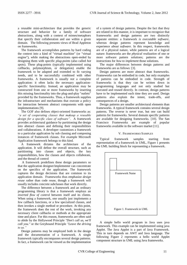
V. FRAMEWORKS SAMPLES
Typical framework samples starting from
representation of a framework in UML, Figure 1 presents
the UML building block for representing a framework.
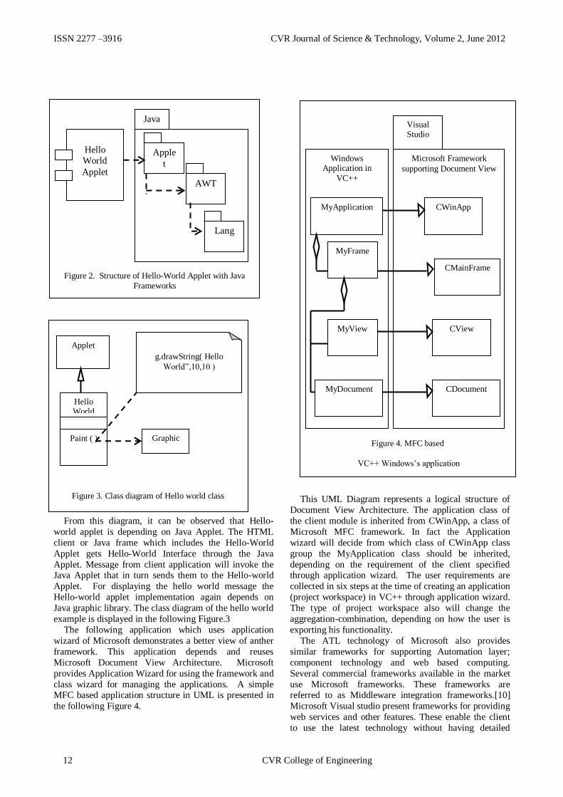
A simple hello world program in Java uses java
framework. This example can be implemented using java
Applet. The Java Applet is a part of Java Framework.
This in turn depends on AWT and Java language. The following Figure 2 represents a hello world Applet
component structure in UML using Java frameworks.
Figure 1. Framework in UML
Framework Name
CVR College of Engineering 11
ISSN 2277 –3916 CVR Journal of Science & Technology, Volume 2, June 2012
From this diagram, it can be observed that Hello-
world applet is depending on Java Applet. The HTML
client or Java frame which includes the Hello-World
Applet gets Hello-World Interface through the Java
Applet. Message from client application will invoke the Java Applet that in turn sends them to the Hello-world
Applet. For displaying the hello world message the
Hello-world applet implementation again depends on
Java graphic library. The class diagram of the hello world
example is displayed in the following Figure.3
The following application which uses application
wizard of Microsoft demonstrates a better view of anther
framework. This application depends and reuses
Microsoft Document View Architecture. Microsoft
provides Application Wizard for using the framework and
class wizard for managing the applications. A simple MFC based application structure in UML is presented in
the following Figure 4.
This UML Diagram represents a logical structure of
Document View Architecture. The application class of
the client module is inherited from CWinApp, a class of
Microsoft MFC framework. In fact the Application
wizard will decide from which class of CWinApp class
group the MyApplication class should be inherited,
depending on the requirement of the client specified through application wizard. The user requirements are
collected in six steps at the time of creating an application
(project workspace) in VC++ through application wizard.
The type of project workspace also will change the
aggregation-combination, depending on how the user is
exporting his functionality.
The ATL technology of Microsoft also provides
similar frameworks for supporting Automation layer;
component technology and web based computing.
Several commercial frameworks available in the market
use Microsoft frameworks. These frameworks are referred to as Middleware integration frameworks.[10]
Microsoft Visual studio present frameworks for providing
web services and other features. These enable the client
to use the latest technology without having detailed
Figure 2. Structure of Hello-World Applet with Java
Frameworks
Hello
World
Applet
Java
Apple
t
AWT
Lang
Figure 3. Class diagram of Hello world class
Applet
Hello World
Paint ( ) Graphic
g.drawString( Hello
World”,10,10 )
Figure
4:
Figure 4. MFC based
VC++ Windows‟s application
Visual Studio
Microsoft Framework
supporting Document View
Windows Application in
VC++
MyApplication
MyFrame
MyView
MyDocument
CWinApp
CMainFrame
CView
CDocument
12 CVR College of Engineering

ISSN 2277 –3916 CVR Journal of Science & Technology, Volume 2, June 2012
knowledge of the hidden technology. Such frameworks
enable common use to use complex technology.
Benefits of Object Oriented Application Frameworks
are Modularity, Reusability, Extensibility, and Inversion
of control. Some of the Challenges of Object Oriented
Application Frameworks are Development efforts,
Learning curve, Integratability, Maintainability,
Validation and defect removal.
VI. OBJECT ORIENTED GRAPHIC FRAMEWORKS
Several pattern languages are available for handling
the problems and for documenting and communicating the skill set of a Graphic and CAD developer. A simple
graphic framework known as pattern-frame for
integrating existing graphic libraries with Microsoft ATL
framework is presented briefly as an example.
Name: Middleware integration pattern-frames
Intent: To export object oriented framework into
component oriented framework using middleware
frameworks.
Motivation and Applicability: The object oriented
graphic frameworks require to be ported into new
technology component-oriented technology for providing better interfaces to the client.
In this pattern frame, the object oriented frameworks is
ported into component-oriented frameworks through
integrating middleware frameworks for supporting
component technology.
Structure: The structure of these frameworks is
presented in the following UML diagram presented in the
Figure 5.
Participants and collaboration: Figure 5. presents
mainly three participants.
1. The object oriented frameworks: They are some of the object oriented frameworks, which need
to be ported to component technology. In this
example a three dimensional object oriented
graphic framework with all user required
graphic functionality (domain specific
functionality) is selected for porting in to COM
technology.
2. The Middleware Integration frameworks: These
frameworks defines interface for exporting the
functionality of object oriented framework and
aggregate the object oriented frameworks to
form black box. They will depend on Middleware component frameworks like
Microsoft ATL, and Java beans frameworks.
They basically provide automation layer. Few
VB command are presented in table 1.
3. The Middleware component framework: This is
a framework used to build components,
supporting component technology. Examples of
middleware component frameworks are Java
Beans development kit, Microsoft Active
Template Libraries.
A. Implementation and Code:
The selected object oriented graphic framework can be
exported to VB client using Active X controls. Building
a graphic component is possible by integrating traditional
graphic framework with Active X controls, which is a
middleware framework. This will export traditional
graphic framework functionality to VB client. Table1
shows sample VB front-end application commands used to control the graphic component frameworks. Sample
view of the e VB application is presented in the Figure 6.
HGP3D1 is the name of the framework component.
Table I.
Few VB Statements used in the application
HGP3D1.Sp3d Text1.Text, Text2.Text, Text3.Text, Text4.Text
HGP3D1.RoteteSegmentAbs Text7.Text, Text4.Text,
Text5.Text, Text6.Text
HGP3D1.ShowAll
HGP3D1.CloseSegment Text7.Text
HGP3D1.RotateSegRel Text7.Text, Text4.Text, Text5.Text,
Text6.Text
Figure 5: Middleware integration based
frameworks
Object Oriented
Frameworks
Middleware Interaction
framework for components
Component based Graphic System
Middleware Component
Frameworks
CVR College of Engineering 13

ISSN 2277 –3916 CVR Journal of Science & Technology, Volume 2, June 2012
Figure: 6 A Three Dimensional graphic Framework
A sample output of the application used to simulate
PCB board using same framework is presented in the
following Figure 7.
Figure 7. A graphic Frameworks for simulating PCB
Several framework patterns for the development of
Graphic frameworks are presented in the following
section.
VI. PATTERN LANGUAGE FOR GRAPHIC
FRAMEWORK
Problems in evolving Graphic frameworks can be
documented adapting pattern approach for provide
solutions. Sixteen typical common design and
implementation issues are identified and they are
classified into three groups depending on nature of the issues namely object oriented, component oriented and
distributed & web based pattern frames. The following
are a catalog of few pattern frames [10].
A. Object Oriented pattern Frames
These are based on simple object oriented patterns. They make lightweight frameworks. They provide
solutions for under engineering problems for developing
frameworks.
Table II.
Object Oriented Pattern Frames
Name Intent
TRADITIONAL
GRAPHIC
FRAMEWORKS
This will apply traditional graphic
techniques for building frameworks
FUNCTION CLASS
FRAMEWORKS
This will apply basic object oriented
patterns for building configurable
function classes
FOUNDATION CLASS
FRAMEWORKS
This will provide hot spot object libraries
for reusing most common modules of the
domain
WHITE -BOX
FRAMEWORKS
This will generate object library for
configurable generic domain specific
classes
FLYWEIGHT OBJECT
FRAMEWORKS
This will decrease number of classes and
number of objects in a system
B. Component Oriented Pattern Frames
These frameworks are based on Component
technology. All are black box frameworks. They provide
solutions for building Component based application
frameworks.
Table III.
Component Oriented Pattern Frames
Name Intent
MIDDLEWARE
INTEGRATION
BASED
FRAMEWORKS
This will reuse middleware integration
frameworks for building Enterprise
frameworks
Component based
frameworks
This will apply patterns defined on
components for providing black box
frameworks
Abstract
Component
frameworks
This will generate black box framework
components using simple object oriented
primitive patterns
Component wrapper
frameworks
This will apply simple object oriented
primitive patterns for using black box
frameworks
C. Distributed nad Webbased Pattern Frames
These are useful for building frameworks for
supporting typical distributed and web based application
requirements.
Table IV.
Distributed Web based Pattern Frames
Name Intent
DISTRIBUTED
FRAMEWORKS
This will provide environment for
building domain specific distributed
application components
WEB ENABLED
FRAMEWORKS
This will provide environment for
building web enabled applications
WEB BASED
FRAMEWORKS
This will provide environment for
building web based applications
14 CVR College of Engineering

ISSN 2277 –3916 CVR Journal of Science & Technology, Volume 2, June 2012
The catalog of frameworks listed above form a pattern
language for building frameworks. Some of the
frameworks are more general in the sense that they are
applicable in other domains. But a few frameworks are
specific to Graphic, CAD and GIS systems. This pattern
language starts its journey from a simple function country
to a complex component world.
CONCLUSIONS
The pattern methodology is useful for documenting,
communicating skill set of expert knowledge for the
purpose of reuse. Development of patterns, pattern
languages and frameworks are essential for every domain for enabling complex technology useful to common user
and for the reuse and communication of domain expert
skill set.
Using pattern at unrequited conditions create over
engineering problem. Not adapting any such methods
leads to under engineering problems. Extreme
Programming referred as XP provides solutions for such
problems.
REFERENCES
[1] Christopher Alexander, “An Introduction for Object- oriented Design”, A lecture Note at Alexander Personal web site www.patternlanguage.com.
[2] Pattern Languages of Program Design. Edited by James O. Coplien and Douglas C. Schmidt. Addison-Wesley, 1995.
[3] Erich Gamma, Richard Helm, Ralph Johnson, and
John Vlissides, "Design Patterns: Elements of Reusable Software Architecture", Addison-Wesley, 1995.
[4] LNCS Transactions on Pattern Languages of Programming http://www.springer.com/computer/lncs?SGWID=0-164-2-470309-0.
[5] Foote B, Yoder J. “Attracting Reuse”. Third Conference on Pattern Languages of Programs
(PLoP'96), Monticello, Illinois, September 1996 [6] Foote B, Opdyke W. „Life Cycle and Refactoring
Patterns that Support Evolution and Reuse‟. First Conference on Pattern Languages of Programs (PLoP‟94). Monticello, Illinois, August, 1994.
[7] Roberts,Don, et Ralph Johnson, Evolving Frameworks A Pattern Language for Developing Object-Oriented Frameworks, Proceedings of Pattern
Languages of Programs, Allerton Park, Illinois, September 1996 (PLoP '96), Addison-Wesley, 1997.
[8] “CHECKS Pattern Language of Information Integrity” at http://c2.com/ppr/checks.html.
[9] Durham A, Johnson R. “A Framework for Run-time Systems and its Visual Programming Language”. Proceedings of OOPSLA ‟96, Object-Oriented Programming Systems, Languages, and Applications.
San Jose, CA. October 1996. [10] Dr.Hari Ramakrishna, “Design Pattern for
Graphic/CAD Frameworks”, Ph.D thesis submitted to Faculty of Engineering Osmania University March 2003, “Architecture of the San Francisco frameworks”–IEEE
eeexplore.ieee.org/iel5/5288519/5387143/05387145.pdf.
[11] Dirk Riehle and Heinz Züllighoven "Understanding and Using Patterns in Software Development" http://www.ubilab.com/publications/print_versions/pdf/tapos-96-survey.pdf.
CVR College of Engineering 15

ISSN 2277 –3916 CVR Journal of Science & Technology, Volume 2, June 2012
Applying Principles Of Lean In Academic
Environments S.Suguna Mallika
CVR College of Engineering, Department of CSE, Ibrahimpatan, R.R.District, A.P., India
Email: [email protected]
Abstract-“Lean is a philosophy that shortens the
time line between the customer order and the
shipment by eliminating waste.” Lean is
principally associated with manufacturing
industries but can be equally applicable to both
service and administration processes. Business
professionals from all over the world have been
studying lean principles for many years and have
enjoyed tremendous bottom-line improvements by
adhering to them. From the production line worker
to the board of directors, everyone in an
organization can benefit. Generally associated with
manufacturing environments, lean is much more
than a manufacturing strategy. Although its roots
lie in manufacturing operations, lean is a business
philosophy that can be practiced in all disciplines
of an organization. This philosophy offers powerful
benefits to enterprise employees, upstream
suppliers, and downstream customers. The need
for external collaboration is absolutely vital to a
lean enterprise because all activities must be
viewed holistically for true success.
Lean manufacturing is underpinned by 5
principles: Specifying what creates value from the
customer’s perspective, identifying all the steps
along the process chain, making those processes
flow, making only what is pulled by the customer,
striving for perfection by continually removing
wastes.
Index Terms-lean, lean in academic, principles of
lean, TPS, and reduce waste.
I. INTRODUCTION
Quality in a software product can be improved
by process improvement, because there is a
correlation between processes and outcomes. As
defined by IEEE, process is ―a sequence of steps
performed for a given purpose.‖ It provides
project members a regular method of using the
same way to do the same work. Process
improvement focuses on defining and continually improving process. Defects found in
previous efforts are fixed in the next efforts.
There are many models and techniques for
process improvement, such as CMMI, ISO9000
series, SPICE, Six Sigma, etc.
Lean philosophy is to maximize customer
value by eliminating waste and optimizing the
existing processes in all aspects of a firm‘s
production activities: human relations, vendor
relations, technology, and the management of
materials and inventory. Lean means doing more
with less effort. Lean Organization understands
customer value and focuses their key processes
in meeting customer needs. Considers an ‗end to
end‘ value stream that delivers competitive advantage. Seeks fast flexible flow.
Eliminates/prevents waste (Muda).Extends the
Toyota Production System (TPS).
II. HISTORY
Toyota first caught the world‘s attention in the
1980s, when it became clear that there was
something special about Japanese quality and
efficiency. Japanese cars were lasting longer than
American cars and required much less repair.
And by the 1990s it became apparent that there
was something even more special about Toyota compared to other automakers in Japan
(Womack, Jones, and Roos, 1991). It was not
eye-popping car designs or performance—
though the ride was smooth and the designs often
very refined. It was the way Toyota engineered
and manufactured the autos that led to
unbelievable consistency in the process and
product. Toyota designed autos faster, with more
reliability, yet at a competitive cost, even when
paying the relatively high wages of Japanese
workers. Equally impressive was that every time
Toyota showed an apparent weakness and seemed vulnerable to the competition, Toyota
miraculously fixed the problem and came back
even stronger. Today Toyota is the third-largest
auto manufacturer in the world, behind General
Motors and Ford, with global vehicle sales of
over six million per year in 170 countries [2].
III. METHODOLOGY
Lean manufacturing is underpinned by 5
principles:
16 CVR College of Engineering

ISSN 2277 –3916 CVR Journal of Science & Technology, Volume 2, June 2012
Specify what creates value from the
customers perspective.
Identify all the steps along the process
chain.
Make those processes flow.
Make only what is pulled by the customer.
Strive for perfection by continually
removing wastes.
The main driver for Lean is to compress the
time period being consumed by a process. In a
conventional supply chain and in individual
businesses, there are potentially huge amounts of
different wastes, known as The 7 Wastes. The 7
wastes are depicted in the above figure as Over
Production, Bad Quality, Operator motion,
Transport, Inventory, Processing, Idle time
et.al.[1]
IV. TOOLS AND TECHNIQUES OF LEAN
A. 5-S principle: The Five S's of Lean
Lean is an approach to process improvement
that is well-known in manufacturing, but which
can be applied to any process. These "S's" originated in Japan, and help build an
environment conducive to a smooth-running
process [3].
B. Sort
Begin by eliminating unnecessary items from
the work area. "Red Tagging" is an effective visual method used to identify unneeded items,
which can then either be moved to a central
holding area or discarded completely. This step
frees up valuable floor space, removes broken or
obsolete tools and fixtures, and makes it easier to
focus on the job.
C. Set in Order
The second S focuses on careful storage so the
job can be carried on effectively. Some questions
that must be posed are
- What do I need to do my job?
- Where should I locate this item?
- How many of this item do I need? Other strategies for Set in Order are painting
schemes that support the work, outlining work
areas, shelving and cabinets for necessary items,
and standard places for tools and materials
needed every day. "A place for everything and
everything in its place" is the essence of this ‗S‘.
D. Shine
Once the first two steps are completed, and
the work space is clear with needed work items
in their places, it's time to thoroughly clean the
work area. Because a clean and orderly area
makes work easier, raises morale, and really
helps staff take pride and ownership in their
work and work space. A clean area also makes it
easier to spot leaks, deterioration of equipment,
misalignments, and broken parts that ultimately
lead to equipment failure and loss of production. The impact of the clean work space will show
itself in several ways on the bottom line.
E. Standardize
This step should always involve the staff from
the job or area. There are always best practices
within a work function, and the first step is to find these practices and bring them to the table.
The staff discusses these and come to agreement
as to the best, making these the standard for all
work in that particular area. But don't stop with
internal best practices, encourage staff to look
outside the company, even in other industries.
Southwest Airlines benchmarked the Woods
Brothers pit team in NASCAR to see how their
fast, effective turnaround of vehicles might have
application in the airlines.
F. Sustain
This last step aims at keeping the new changes
in place, and it's the toughest to implement.
Because people build habits, and even when
those habits are tied to poor methods of work,
they're used to them and find it hard to change.
Find ways to reward maintenance of these new changes, especially during the first 3 months.
CVR College of Engineering 17

ISSN 2277 –3916 CVR Journal of Science & Technology, Volume 2, June 2012
V. LEAN IN ACADEMIC ENVIRONMENTS
A. Case Study 1
Lean can also be applied in the academic
environments. Consider taking the example of
academic administration. There are many
challenges faced by the academic administration
like ―absenteeism of students‖. One of the tools
of Lean can be used to mitigate this by the use of
Visual Control Boards in the classrooms. This
visual control boards should be placed for every
class which is divided into parts specifying the
names of the list of students who are below the threshold level of attendance and on the other
side list of students who are holding the highest
attendance. This certainly impacts the
endangered students in correcting their
attendance and motivates the regularly coming
students to be more regular. This visual board
could be updated monthly. A sample visual
board could look like as follows:
Low Attendance(Danger)
N.Abhishek-10B83S0213-35%
S.Suma-10B83S0238-63%
Green Zone (Thumbs Up)
P.Sagar-10B83S0215-96%
K.Kamala-10B83S0217-93%
B. Case Study 2
The second case that has been taken into
consideration is the process of conducting the
internal and external examinations for the
students during the academic year. Generally the
process followed is the lab internal takes a print
out of all the programs decided to be part of the
exam and each of the question printout is manually placed in the answer scripts. The
students are then instructed to come into the lab
one at a time in a serial order and each student is
asked to pick up one answer script at random
which would be opened after occupying the
designated seat. The student is instructed to copy
the question into his paper and then supposed to
proceed with the exam. The time duration for
conducting a lab exam is typically 2.5 hours out
of which it is to be understood that by the time
all the students have completed picking up the answer scripts assuming 40sec for each student
making it a total of 40*60 i.e. 24 minutes. So the
average time allotted for the student to complete
the program is getting reduced by 20 minutes.
After a series of discussions and understanding
the flow of the process Lean has been applied to
this process and it has been proposed that the lab
questions should be fed into the server and
randomly the selected question is displayed on the monitor of the system into which the student
logs in directly. This reduces the typical 20
minute delay and thereby increases the
productive utilization of the time slot available.
At the same time stress management can be done
more effectively. While the process was 87%
effective after applying lean philosophy it
becomes 97% effective with an absolute 10%
more utilization and better productivity.
REFERENCES
[1] David.P.Spencer, Gerhard Plenert LEAN on IT: Applying LEAN Manufacturing principles across the IT organization.
[2] Jeffrey K. Liker, The Toyota Way: 14 Management Principles from the World's Greatest Manufacturer.
[3] David Black The 5-S‘s. [4] Womack JP, Jones DT. Lean Thinking:
Banish Waste and Create Wealth in Your Corporation. New York: Simon and Schuster, Inc.; 1996, Second Edition 2003.
18 CVR College of Engineering

ISSN 2277 –3916 CVR Journal of Science & Technology, Volume 2, June 2012
Region-Wise Quality Measurements Of Pan-
Sharpened Images G.P.Hegde
1, Dr.I.V.Muralikrishna
2, Dr.Nagaratna Hegde
3
1SDM Institute of Technology, Department of CSE, Ujire, India
Email: [email protected] 2JNTUH, Hyderabad, A.P., India
Email: [email protected], 3Vasavi College of Engineering, Hyderabad, A.P., India
Email:[email protected]
Abstract- Image pan-sharpening or data fusion is widely used
method for increasing the spatial resolution of multispectral
images. Hence, the task is to enhance the spatial resolution of
the multispectral images by merging them with spatially more
highly resolved panchromatic data obtained from a satellite
sensor. However, the analysis of quality distortion of the final
pan-sharpened image is a difficult task in the field of remote
sensing, since a reference image is usually unavailable. This
paper illustrates the measurement of spectral and spatial
quality of pan-sharpened images region-wise using object
based image segmentation technique. Experimental results
show that the proposed pan-sharpening scheme can effectively
preserve spectral information while improving the spatial
quality, and outperforms the general IHS based pan-
sharpening methods.
Index Terms: Image pan-sharpening, IHSWT, NSCT, and
Segmentation.
I. INTRODUCTION
Image pan-sharpening is a process of enhancing the
spatial features of multispectral images and combining
complimentary contents of source images. The successful
pan-sharpening is of great importance in many applications,
such as military, remote sensing and weather forecasting, et
al. The pan-sharpened image should preserve all relevant
information contained in the source images. Pan-sharpening
process should not introduce any artifacts, which can
distract or mislead human observer. Images used in the pan-sharpening process must be properly preprocessed. This
paper illustrates image segmentation of raw multispectral
image in unsupervised manner.
Fig.1 shows flow of image quality measure of pan-
sharpened or fused images. Low resolution raw
multispectral image is combined with high resolution
panchromatic image hence resolution and spatial quality of
multispectral image is increased. From the literature review
it has been concluded that there is a lack of methods for the
assessment of pan-sharpening algorithms, focusing on both
spectral and spatial quality evaluation. Thus, image
segmentation and estimation of the sharpening or fusion performance is still an open problem, which needs more
attention from the scientific community. Analysis of image
pan-sharpening would helps in image classification due to
availability of spectral and spatial quality of images.
Figure 1: Image pan-sharpening and measurement of quality preservations
II. METHODS OF IMAGE PAN SHARPENING
In this paper, Brovey transform based image pan-
sharpening, Intensity Hue Saturation (IHS) based pan-
sharpening, Principal Component Analysis (PCA)
transform based image pan-sharpening, Intensity Hue
Saturation Wavelet Transform (IHSWT) based pan-
sharpening methods are briefly explained. Performance of
all these four methods are evaluated and compared with
IHSNSCT proposed pan-sharpening method.
A. Brovey Transformation Based Pan-sharpening
Brovey transform is a simpler but widely-used in RGB
color fusion. The algorithm decomposes the phase space of
the multi-spectral image into 3 color regions. Brovey
Transform based on numerical methods involves taking a
product of the DN value of the high resolution image and
the normalized DN value of the three bands of the multispectral image. In Brovey transform based pan-
sharpening method, three regions are obtained according to
the following:
CVR College of Engineering 19

ISSN 2277 –3916 CVR Journal of Science & Technology, Volume 2, June
2012
(1)
(2)
(3)
In equation 1,2,3 formula, R stands for the red band of
multi-spectral image, G stands for the green band of multi-
spectral image, B stands for the blue band of multi-spectral
image, and PAN stands for the intensity value of high spatial resolution image. In addition, Brovey transform
need better pretreatments and noise filtering in order to
reduce redundant data and non-spectral information. The
Brovey transform was developed to increase the contrast in
low and high ends of histogram of an image and produce
visually appealing images. Consequently, the Brovey
transform should not be used if the preservation of the
original scene radiometry is important. The Brovey
transform is, however, applicable only to images with three
bands. It preserves the spatial characteristics to a large
extent. This method preservers spatial information of pan-
sharpened image.
B. Intensity Hue Saturation Based Pan-sharpening
It uses three positional parameters in lieu of the Red,
Green and Blue (RGB) such as Intensity, Hue and
Saturation. Intensity relates to the overall brightness of a
color or energy level of the light. Hue component indicates to the dominant or average wavelength of light contributing
to a color, i.e. the actual perceived color such as red, blue,
yellow, orange, etc. Saturation specifies the degree to which
the color is pure from white light (grayscale) dilution or
pollution. It runs from neutral gray through pastel to
saturated colors. The transformation from RGB color space
to IHS space is nonlinear, lossless and reversible. It is
performed by a rotation of axis from the first orthogonal
RGB system to a new orthogonal IHS system. The
equations describing the transformation of RGB color
regions into the IHS regions (Pellemans, et al., 1993). This
transformation permits the separation of spatial information into one single intensity band.
Converting colors from RGB to HIS: Given an image
RGB color format, the H component of each RGB pixel is
obtained using the equation 4.
(4)
With
The saturation component is given by equation 5.
(5)
Finally, the intensity component is given by equation 6.
(6)
It is assumed that the RGB values have been
normalized to the range [0,1] , and that angle is measured with respect to the red axis of the IHS space , Hue can be
normalized t o the range [0,1] by dividing by 3600 all
values resulting from the equation for H. The other two IHS components already are in this range if the given RGB
values are in the interval [0,1].
Converting colors from IHS to RGB: Given values of
IHS in the interval [0,1], corresponding RGB values in the
same range is calculated by the equations 7 to equation 17.
The applicable equations depend on the values of H. By
multiplying H by 3600 which returns the hue to its original
range of [0, 3600].
RG sector (00 H 1200)
(7)
(8)
And
(9)
GB sector (1200 H < 2400) If the given value of H is in this sector, we first subtract 1200 from it.
(10)
Then the RGB components are
(11)
(12)
20 CVR College of Engineering

ISSN 2277 –3916 CVR Journal of Science & Technology, Volume 2, June
2012
And
(13)
BR sector (2400 H 3600).Finally, if H is in this range, then 2400 is subtracted from it
(14)
Then the RGB components are
Figure 2: Schematic diagram of IHS method of pan-sharpening
(15)
Where
(16) And
(17)
A variation of the IHS value is computed as the
average of the maximum and minimum values of the R, G,
and B channels in the multispectral image. Fig 2 shows
schematic diagram of IHS based pan –sharpening method.
C. Principal Component Analysis
The PCA transform converts inter-correlated
multispectral bands into a new set of uncorrelated
components. It is assumed that the first PC image with the
highest variance contains the most amount of information
from the original image and will be the ideal choice to replace the high spatial resolution panchromatic image. All
the other multispectral bands are unaltered. An inverse PCA
transform is performed on the modified panchromatic and
multispectral images to obtain a high-resolution pan-
sharpened image. Principal component transform (PCT)
based on the PCA proceeds through conversion of a set of
multispectral bands (three or more bands) into a set of
principal components. Pohl (1996) reported that the PCA
method preserves the original spectral resolution. The PCA
is capable of mapping most of the information (variance)
within all bands into the first principal component. The
spectral information unique to any band then gets mapped
to the other principal components (Chavez et al 1991,
Jensen 1996). The first PC component is then replaced by
the panchromatic component because the first PC image is
representative of the spectral information of the
multispectral image. Finally a reverse principal component
transformation takes place to convert the replaced
components back to the original image space. The PCA
method can be used for more than three bands. Fig. 3 shows
the Schematic diagram of PCA method.
Figure 3:.Schematic diagram of PCA method of pan-sharpening
The equation18 is used to compute the PC components
from 3 bands of the MS image.
=
(18)
Where each row in the transformation matrix in equation
18 represents the eigen vectors of the covariance matrix. To
convert back to the RGB space, the transformation is given
by equation 19.
=
(19)
D. Intensity Hue Saturation Wavelet Transform
In this research paper Intensity Hue Saturation wavelet
transform image pan-sharpening method is employed for
fusion of multispectral and panchromatic images. Nunez et
al. presented a multi-resolution-based image fusion method
with additive wavelet decomposition. The discrete wavelet transform known as “a trous” algorithm was used to
decompose the images. The “a trous” algorithm is also
called the intensity hue saturation wavelet transform
(IHSWT), which provides a shift-invariant property that is
not available with the ortho normal wavelet system.
Additive and substitution are two different combination
methods for image sharpening. In the substitution method,
both the resampled multispectral and panchromatic images
were decomposed into the wavelet domain. The low
resolution component of the panchromatic image was then
CVR College of Engineering 21

ISSN 2277 –3916 CVR Journal of Science & Technology, Volume 2, June
2012
substituted using the low resolution component of each MS
band to produce new sharpened MS bands. The high
frequency wavelet planes corresponding to the MS image
are discarded and are replaced by the high frequency
wavelet planes of the panchromatic image. In the additive
method, the high resolution detail components of the
panchromatic image were added to each of the MS bands or
to the intensity component of the IHS transformed MS
bands. The additive method uses all the spectral
information available in the MS image and adds the high
frequency planes from the panchromatic image. Also, adding the high frequency component only to the intensity
component preserves the spectral information available in
the image data. The sharpening method was applied to
sharpen the MS bands of IRS 1D LISS III using the IRS 1D
panchromatic image [8].
King et al. introduced a wavelet based sharpening
method that uses IHS transformation and biorthogonal
wavelet decomposition. The process flow diagram of the
sharpening method is shown in Fig. 4. The MS image bands
are first transformed into intensity, hue, and saturation
bands. The panchromatic image is histogram matched with the intensity component. The histogram matched
panchromatic image is expanded in the wavelet domain
using the biorthogonal as the mother wavelet.
The intensity component replaces the low-resolution
approximation of the panchromatic image in the wavelet
domain. The inverse discrete wavelet transformation
(DWT) is done to obtain a fused intensity component where
the high frequency details are added to the intensity
component. The hue and saturation components are
resampled to the size of the sharpened intensity band. The
inverse IHS transformation is done to get back to the RGB image domain. A wiener filter is applied to remove noise
from each band of the sharpened image. The design of the
orthonormal wavelet system is complicated. Linear phase
symmetric filters are not possible with orthonormality
condition. They are also not shift invariant. The linear
phase characteristic of the wavelet filters is a desirable
property for many applications. The biorthogonal wavelet
systems lift orthonormality constraints to obtain symmetric
filters that provide perfect reconstruction. The biorthogonal
systems use two different bases, one is the dual of the other.
Figure 4. Flow diagram of the IHSWT based sharpening
The merged image is filtered using an adaptive wiener
filter. The width of the linear structures should approach the
width seen in the panchromatic image. The wiener filter is
used to smooth the excess edges in the sharpened data and
additive noise. The wiener filter is an optimal linear filter
used to filter images degraded by additive noise. The filter
performance is based on the image variance. The adaptive
filter is more suitable compared to the linear filter. The
wiener filter performs a small amount of smoothing if the
local variance is high. If the local variance is small, the
filter performs more smoothening so that excess edges are removed.
E. Intensity Hue Saturation Combined with
Nonsubsampled Contourlet Transformation
IHSNSCT is a proposed image pan-sharpening
method in this research study. This method is surpassing
the problem overcome by wavelet transformation methods. Wavelet transformation based image sharpening methods
are not effective in representing the spatial information’s
like geometrical smoothness of the contours. Wavelet
transformation methods can preserve large amount of
spectral information of image but it cannot preserve huge
amount of spatial contents. Images obtained from satellite
scanners may have number of spatial information’s some of
them are extracted by enhancing and sharpening the edges,
boundaries, smooth regions and smooth curves which
cannot be efficiently captured by the wavelet transform. In
order to overcome this problem IHS+NSCT method is used. The Nonsubsampled Contourlet Transform
(NSCT)[2] combines nonsubsampled pyramids (NSP) and
non-subsampled directional filter bank (NSFB’s.). The
pyramids provide multiscale decomposition and the
NSFB’s provide directional decomposition. This process is
iterated repeatedly on the lowpass subband outputs of
nonsubsampled pyramids resulting in the Non-subsampled
Contourlet Transform (NSCT). This method is especially
yields better results for edges and contours than discrete
wavelet transformation technique. The core of the NSCT
technique is the non-separable two-channel nonsubsampled
filter banks. It is easier and more flexible to design the needed filter banks that lead to a NSCT with better
frequency selectivity and regularity when compared to the
contourlet transform. A general scheme for the IHS+NSCT
based pan-sharpening methods is shown in Fig.5. This
method can be performed in the following steps:
i) Find intensity, hue, saturation components from
input raw multispectral input (MS) image. Apply
the gamma correction for Intensity component.
ii) Panchromatic (PAN) image is histogram matched
with gamma corrected intensity component, hence
new histogram matched PAN image is obtained (IPAN). Apply the NSCT enhance method for this
intensity (I) component and also for the histogram-
matched PAN image (IPAN) for N, levels
22 CVR College of Engineering

ISSN 2277 –3916 CVR Journal of Science & Technology, Volume 2, June
2012
(decompose both the images and find NSCT
coefficients).
iii) Estimate the noise standard deviation of I
component and also for histogram matched PAN
Image (IPAN).
iv) For each level DFB,
a) Estimate the noise variance
b) Compute threshold and the amplifying ratio.
c) At each pixel, compute the mean and the
maximum magnitude of all directional subbands at
this level, and classify into strong edges, weak edges or noises.
d) For each directional subband, use the non linear
mapping function to modify the NSCT coefficients
according to the classification.
v) Fuse the detail and approximate coefficients of the
intensity component and IPAN using equation 20.
+
(20)
vi) Apply the inverse NSCT to the fused detail and
approximate coefficients to reconstruct the new
intensity component Inew
vii) Perform the inverse HIS transform to the new
intensity component, new I together with hue and
saturation components to obtain the new RGB or
fused image.
III. IMAGE SEGMENTATION
This procedures partition an image into its constituent parts or objects. A rugged segmentation procedure brings
the process a long way towards successful solution of
imaging problems that require objects to be identified
individually. Proposed Image segmentation technique is an
object based technique which generates regions with same
spatial characteristic. This technique uses the spatial
variability in the image for region generation.
Figure.5: Schematic diagram of IHS+NSCT method of pan-sharpening
A. Object Based Image Segmentation
The image contents or objects can be enhanced using
image pan-sharpening by increasing the spatial resolution
of such images and also preserving the spectral contents.
The degradation factor and enhancement factor of images are considered to measure spectral and spatial changes
between the original multispectral image m and the pan-
sharpened product mf. However, careful investigations
showed that the performance of the pan-sharpening method
is always region-based and highly dependent on the actual
scene content.
A measure to determine the spatial variability of the
scene is needed. The standard deviation of the pixels’
values inside a square window was chosen for this purpose
since it represents the scatter of the data [1]. We use a
sliding window with the size of 3×3 pixels and assign the standard deviation value inside the window to the central
pixel as a salience measure of this region. Pixels with high
values represent regions with high variability of the spatial
data in the original image, whereas low values account for
homogeneous areas.
The newly created image is denoted as fσ as in equation
21.
(21)
Where
=
And n is the number of pixels inside the window W(x,y). The next step is to segment fσ in order to mark regions with
similar spatial characteristics. An example for the
histogram of typical fσ is shown in Fig. 6.
Figure 6. Histogram of typical fσ
CVR College of Engineering 23

ISSN 2277 –3916 CVR Journal of Science & Technology, Volume 2, June
2012
From the above histogram two thresholds th1 and th2 are
defined. The pixels with values less than th1 are considered
to represent homogeneous areas similarly pixels with values
larger than th2 represent heterogeneous regions with the
extreme variability of the spatial features. The pixels with
values between th1 and th2 indicate areas with moderate
salience. For the test cases the corresponding histograms of
the fσ resembled Gamma distributions with a confidence
interval of 95%. Thus, thresholds are determined in an
unsupervised fashion by: th1=µ(fσ)−σ(fσ), th2=µ(fσ)+σ(fσ),
where µ denotes the mean and σ denotes variance of fσ. After the process of thresholding, three individual binary
maps with same size as the original multispectral image are
obtained.
B. Content Evaluation of Pan-sharpened Images
1) 1). Spectral Evaluation:Let mi be all the pixels of m which constitute region i with i=1…3, while mfi
are the pixels with the same coordinates as in mi
but from mf. The root mean square of the
differences, i.e. RMS (mfi-m
i), is used to calculate
the spectral changes of three regions
(homogeneous, moderate and highly non-
homogeneous areas).
2) Spatial Evaluation:Measurement of spatial quality
preservation of the pan-sharpened image is a more
complex task and usually based on perceptual
inspection. The alterations of image gradients are
proposed as a measure of spatial changes. The first order derivative gradients are used in edge
detection algorithms since absolute value of the
first derivative tends to be higher in regions with
strong presence of edges. The Roberts cross
difference operator is used to calculate the gradient
values. To calculate spatial changes, initially
Sobel’s gradient operator is applied to both m and
mf. The filtered images are denoted as R(m) and
R(mf), respectively.
Then, sums of the gradients inside the three regions are
calculated individually for both R(m) and R(mf). The normalized difference of the sums is a measure of spatial
enhancement (or degradation), whereby the normalization
is performed with respect to the number of pixels belonging
to the individual region. The final formula for spatial
changes using the Roberts gradient is: [∑Ri(mf)-
∑Ri(m)]/Ni.
IV. ANALYSIS AND RESULTS
Images are used in this study are from Hyderabad
city and its surrounding areas. Remote sensing satellite
images of low resolution multispectral data (IRS 1C LISS
III; 23.5m, 256x256 resolution) and a high resolution
panchromatic data (IRS PAN; 5.8m, 700x700 resolution) are used for image pan-sharpening. Two images are
geometrically corrected using ground control points
extracted from the maps and both these images are fused
together using conventional and non conventional methods
of images sharpening. Before pan-sharpening of images it
must be properly co-registered and resampled. There are
several image sets are tested, but in this paper only one data
set image are shown. Fig 7 shows the source image of
Hyderabad Dist. Fig. 8 shows segmented regions and pan-
sharpened images used in this study. A region value of
input multispectral image is shown in Table 1. Similarly
Fig.9 shows results of spectral quality preservation and
Fig.10 shows results of spatial quality preservation of pan-
sharpened images respectively. From the results we can say that IHSNSCT method of image pan-sharpening preserves
more spectral information and improves spatial quality of
pan-sharpened images than IHS and IHSWT methods.
Index values shown in tables 2 and 3 are quality distortion.
Less value indicates less distortion in the image hence more
quality of image is preserved.
Figure 7. Source Images.
Figure 8. Segmented regions and Pan-sharpened images
24 CVR College of Engineering

ISSN 2277 –3916 CVR Journal of Science & Technology, Volume 2, June
2012
Table I. Region values of input multispectral image
Regions Size
Region1 6743
Region2 49545
Region3 7712
Figure 9. Results of preservation of spectral quality
Figure 10. Results of preservation of spatial quality
CONCLUSIONS
The quality preservation assessment of various image
sharpening methods was performed.. It was observed that
spectral changes are less in HIS methods of pan-sharpening
compare to IHS and IHSWT methods. The spectral changes
are less in conventional pan-sharpening methods like PCA
compared to IHS based methods. The influence of spatial
variations in homogenous region is less during pan-
sharpening process. The amount of more spectral changes
in homogenous regions1 can be accredited to addition of
complementary information during image pan-sharpening.
It is also observed that preservation of spectral and spatial
quality is improved in IHS methods.
Further analysis to determine the direction flexibility
would be appropriate to quantify the significance of
negative values, finally it was concluded that proposed
fusion schemes IHSNSCT and IHSWT can effectively
preserves spatial information compare to IHS method. It
indicates edges and region boundaries are much enhanced
Similarly IHSNSCT and IHSWT method improves the spectral quality of pan-sharpened images. PCA method
preserves more spectral information but disturbs the spatial
quality of images.
REFERENCES
[1] Tremeau, N. Borel, “A region growing and merging algorithm to color segmentation”, Pattern Recognition 30 (7) 1191-1203, 1997.
[2] Bruce King and Vijay Vohora , Lau Wai Leung, Dept of
Land Surveying & Geo-Informatics, The Hong Kong Polytechnic University.“ Comparision of Image Data Fusion Techniques Using Entropy and INI”.,2001.
[3] C.S. Xydeas and V. Petrovic, “Objective image fusion performance measure”, Electronics Letters, vol. 36, no. 4, pp. 308-309, 2000.
[4] D.R. Reddy, R. Ohlander, K. Price, “Picture segmentation using a recursive region splitting method
”, Computer Graphics Image Process. 8 313-333, 1978. [5] D Sinclair, Voronoi “Seeded colour image
segmentation”, Technical Report 3, AT&T Laboratories Cambridge, 1999.
[6] F Pedro. Felzenszwalb, Artificial Intelligence Lab, Massachusetts Institute of Technology. Daniel P. Huttenlocher, Computer Science Department, Cornell University. “Efficient Graph-Based Image Segmentation.2002.
[7] G. Piella and H. Heijmans, ”A new quality metric for image fusion ”,Proc. IEEE International Conference on Image Processing, Barcelona,Spain, pp. 173–176, 2003.
[8] G.Qu, D.Zhang and P.Yan, “Information measure for performance of image fusion”,Electronics Letters,vol. 38, no. 4, pp. 313-315, 2002.
[9] J Francisco. Tapiador, Department of Geography, University of Birmingham “A Multispectral/
Panchromatic Data Fusion Method Based in Jaynes Maximum Entropy”, 2001.
[10] J. P. Lewis, Industrial Light & Magic, “Fast Normalized Cross-Correlation”, 2003.
[11] Jianping Fan, David. K. Y. Yau, Member, IEEE, Ahmed. K. Elmagarmid, Senior Member, IEEE, and Walid G. Aref, Member, IEEE. “Automatic Image Segmentation by Integrating Color-Edge Extraction and
Seeded Region Growing”. [12] J.G.Liu, T.H.Huxley School of Environment, Earh
Science and Engineering, “ Smoothig Filter-based Intensity Modulation : a spectral preserve image fusion technique for improving spatial details ”.
[13] J. Li, “Spatial Quality Evaluation of Fusion of Different Resolution Images”, International Archives of Photogrammetry and Remote Sensing, vol.33 ,2000.
CVR College of Engineering 25
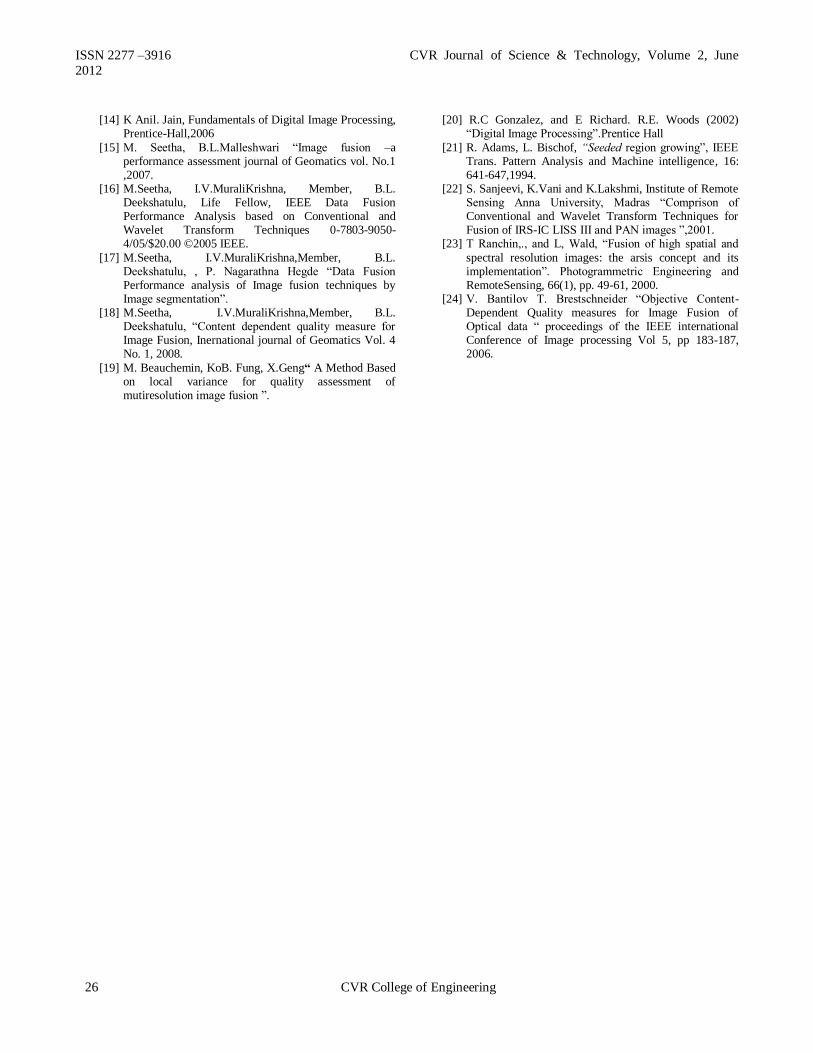
ISSN 2277 –3916 CVR Journal of Science & Technology, Volume 2, June
2012
[14] K Anil. Jain, Fundamentals of Digital Image Processing, Prentice-Hall,2006
[15] M. Seetha, B.L.Malleshwari “Image fusion –a performance assessment journal of Geomatics vol. No.1 ,2007.
[16] M.Seetha, I.V.MuraliKrishna, Member, B.L. Deekshatulu, Life Fellow, IEEE Data Fusion Performance Analysis based on Conventional and Wavelet Transform Techniques 0-7803-9050-4/05/$20.00 ©2005 IEEE.
[17] M.Seetha, I.V.MuraliKrishna,Member, B.L. Deekshatulu, , P. Nagarathna Hegde “Data Fusion Performance analysis of Image fusion techniques by Image segmentation”.
[18] M.Seetha, I.V.MuraliKrishna,Member, B.L. Deekshatulu, “Content dependent quality measure for Image Fusion, Inernational journal of Geomatics Vol. 4 No. 1, 2008.
[19] M. Beauchemin, KoB. Fung, X.Geng“ A Method Based on local variance for quality assessment of mutiresolution image fusion ”.
[20] R.C Gonzalez, and E Richard. R.E. Woods (2002) “Digital Image Processing”.Prentice Hall
[21] R. Adams, L. Bischof, “Seeded region growing”, IEEE Trans. Pattern Analysis and Machine intelligence, 16: 641-647,1994.
[22] S. Sanjeevi, K.Vani and K.Lakshmi, Institute of Remote Sensing Anna University, Madras “Comprison of Conventional and Wavelet Transform Techniques for Fusion of IRS-IC LISS III and PAN images ”,2001.
[23] T Ranchin,., and L, Wald, “Fusion of high spatial and
spectral resolution images: the arsis concept and its implementation”. Photogrammetric Engineering and RemoteSensing, 66(1), pp. 49-61, 2000.
[24] V. Bantilov T. Brestschneider “Objective Content- Dependent Quality measures for Image Fusion of Optical data “ proceedings of the IEEE international Conference of Image processing Vol 5, pp 183-187, 2006.
26 CVR College of Engineering
ISSN 2277 –3916 CVR Journal of Science & Technology, Volume 2, June 2012
Polarization Reconfigurable Microstrip Antennas
For Wireless Communication A. Bharathi
1 and P.Kavitha
2
1CVR College of Engineering, Department of ECE., Ibrahimpatan, R.R.District, A.P., India
Email: [email protected] 2CVR College of Engineering, Department of ECE., Ibrahimpatan, R.R.District, A.P., India
Email: [email protected]
Abstract--Antenna systems that utilize polarization diversity
are gaining popularity due to development of wireless
communication in recent years. This paper presents a novel
polarization reconfigurable antenna to improve the reliability
of wireless communication system. The structure is very
simple obtained by trimming the corners of square patch fed
with microstrip line feed, and adding four small triangular
shape conductors at the corners. Introducing independently
biased pin diodes into the gap between patch and triangular
conductors, the antenna can radiate linear polarization (LP),
or left hand circular polarization (LHCP) or Right hand
circular polarization (RHCP). The proposed antenna designed
for 1.6 GHz range, achieve excellent performance with LP,
RHCP, LHCP at the same frequency and are built on FR4-
Epoxy substrate. The antenna architecture is interesting for
commercial wireless applications because it is compatible with
modern fabrication processes and can be realized on low cost
dielectric materials.
Index Terms—Microstrip antenna, Polarization.
I. INTRODUCTION
Microstrip antennas are widely used in Wireless and
mobile communication systems applications due to their low
profile, light weight, conformable with RF circuitry and
easy fabrication [1]. They are usually designed for single-
mode operation that radiates mainly linear polarization. In
some applications, such as satellite communications,
however, a circularly polarized system is more suitable
because of its insensitivity to transmitter and receiver orientations [2]. In this regard, integrated systems with
different communication networks have attracted significant
attention. To achieve such multi-operation, numerous
researchers have investigated microstrip antennas with
switchable polarization. The switchable property allows the
user to roam any existing network and have only a single
handset to access a great number of services. Therefore, they
can be utilized to realize frequency reuse [3]. Polarization
diversity of reception is important to counter the effects of
fading in communication, especially in mobile
communication [4]. In addition, a microstrip antenna with switchable polarization is very important because many
current communication and sensor systems require a high
degree of polarization control to optimize system
performance [5]. Practical applications of this technique
have been described in [3], [4], and [6]. Based on the same
concept, a novel reconfigurable microstrip antenna allowing
polarization switching is proposed and carefully examined
in this study. Individually biased PIN diodes introduced into
the corners of antennas enable independent control of
polarization sense.
II. RECONFIGURABLE MICROSTRIP PATCH ANTENNA DESIGN
A. Polarization Reconfigurable Patch Antenna Design:
Figure 1. Configuration of the patch antenna with polarization diversity.
Fig. 1 shows the proposed Microstrip antenna with square
patch having a side length of 44.3 mm printed on a substrate
with a relative dielectric constant of 4.4 and thickness of 1.6
mm. Its resonant frequency is 1.6 GHz.
The truncated corners have an equal side length 6 mm
and are used to provide perturbation, so as to obtain two orthogonal near-degenerate resonant modes for circular
polarization. The technique of truncating corners of a square
patch to obtain single-feed circular polarization operation is
well known and has been widely used in practical designs
[7]. This corner-truncated square patch has four small
parasitic conductors of triangular shape with a side length of
2.3 mm. As the size of the PIN diode is 2.5× 1.4 mm, the
gap between the square patch and triangular conductors is
designated as 1.4 mm. The impedance and radiation
properties of reconfigurable patch antenna is investigated
numerically and experimentally. Simulations are carried out using HFSS, a commercial EM Simulator using Finite
Element Method (FEM). The proposed antenna shows
excellent radiation characteristics. The return loss, the gain,
and the radiation patterns of the proposed antenna have been
simulated and measured under different biasing conditions
CVR College of Engineering 27

ISSN 2277 –3916 CVR Journal of Science & Technology, Volume 2, June 2012
of the diodes. Different polarization is achieved by changing
the geometry of antenna according to on/off state of diodes.
Figure shows the configuration of the patch antenna which radiates linearly polarized waves.
TABLE I:
Diode1 Diode2 Diode3 Diode4 polarization
A1 ON ON ON ON LP
A2 ON OFF ON OFF LHCP
A3 OFF ON OFF ON RHCP
The resonant frequency remains same as 1.6 GHz for all
the three polarizations (LP, RHCP, LHCP). The diode configurations are shown in Table I. for different states of
polarization.
Fig. 2 shows the return loss and axial ratio plots for LP
state when all the four diodes are on. A -10dB return loss is
obtained at resonant frequency with an Axial Ratio of 41
dB.
Figure 2 Simulated results for (a) Return loss and
(b) Axial ratio giving LP when all the diodes are on.
Fig. 3 shows the return loss and axial ratio plots for
LHCP when diode1 and diode 3 are on. A -10dB return loss
is obtained at resonant frequency with an Axial Ratio of 1.5
dB.
Figure 3. Simulated results for (a) Return loss and (b) Axial ratio
giving CP when diode 1 and diode 3 are on.
Figure 4. Simulated results for (a) Return loss and (b) Axial ratio giving CP when diode 2 and diode 4 are on.
28 CVR College of Engineering
ISSN 2277 –3916 CVR Journal of Science & Technology, Volume 2, June 2012
Fig. 4 shows the return loss and axial ratio plots for
RHCP when diode2 and diode 4 are on. A -10d B return loss is obtained at resonant frequency with an Axial Ratio of 2
dB.
CONCLUSIONS
A Microstrip antenna with switchable polarization at
1.6GHz is presented. It shows different polarizations
achieved by using pin diodes. It has uniplanar design which
allows integration of active/passive elements. It can be used
in applications where polarization diversity is required.
Without any change in feed mechanism the antenna can
radiate LP, RHCP and LHCP by controlling bias voltage.
This design has desirable features for wireless
communication applications such as WLAN, Satellite Links and Space Robots.
REFERENCES
[1] J. R. James, P. S. Hall, and C. Wood, Microstrip Antenna
Theory and Design. London, U.K.: Peter Peregrinus, 1981.
[2] F.-S. Chang, K.-L. Wong, and T.-W. Chiou, “Low-cost broadband circularly polarized patch antenna,” IEEE Trans. Antennas Propagat., vol. 51, pp. 3006–3009, Oct. 2003.
[3] F. Yang and Y. Rahmat-Samii, “A reconfigurable patch antenna using switchable slots for circular polarization
diversity,” IEEE Microwave Wireless Compon. Lett., vol. 12, pp. 96–98, Mar. 2002.
[4] M. K. Fries, M. Grani, and R. Vahldieck, “A reconfigurable slot antenna with switchable polarization,” IEEE MicrowaveWireless Compon. Lett., vol. 13, pp. 490–492, Nov. 2003.
[5] K. C. Gupta and P. S. Hall, Analysis and Design of Integrated Circuit Antenna Modules. New York: Wiley,
2000. [6] P. M. Haskins, P. S. Hall, and J. S. Dahele,
“Polarization-agile active patch antenna,” Electron. Lett., vol. 30, pp. 98–99, Jan. 1994.
[7] W.-S. Chen, C.-K. Wu, and K.-L. Wong, “Novel compact circularly polarized square microstrip antenna,” IEEE Trans. Antennas Propagat., vol. 49, pp. 340–342, Mar. 2001.
CVR College of Engineering 29

ISSN 2277 –3916 CVR Journal of Science & Technology, Volume 2, June 2012
Technology Scaling And Low Power Design
Techniques T.Esther Rani
1, Dr. Rameshwar Rao
2 and Dr.M.Asha Rani
3
1CVR College of Engineering, Department of ECE., Ibrahimpatan, R.R.District, A.P., India
Email: [email protected] 2Hon‘ble VC, JNT University, Hyderabad, India
Email:[email protected] 3JNT University, Department of ECE, Hyderabad, A.P., India
Email: [email protected]
Abstract —Scaling the feature size of transistor made a
remarkable advancement in silicon industry. The demand
for power-sensitive design has grown significantly in recent
years due to growth in portable applications. The need for
power-efficient design techniques is increasing. Various
efficient design techniques have been proposed to reduce
both dynamic as well as static power in state-of-the-art
VLSI applications. In this paper, different circuit design
techniques both static and dynamic are discussed that
reduce the power consumption.
Index Terms—Scaling, feature size, power-efficient, design
techniques.
I. INTRODUCTION
In the past, the major concerns of the VLSI designer
were area, performance, cost, reliability. Power consideration was mostly of secondary importance. In
recent years this has begun to change. Power is being
given comparable importance to area and speed. Several
factors have contributed to this trend. The primary
driving factor has been a remarkable success in terms of
growth of the class of personal computing devices and
wireless communications systems, which demand high-
speed computation and complex functionality with low
power consumption. The semiconductor industry has
witnessed the growth in demand and supply of portable
systems in consumer electronics market. High performance portable products, ranging from small hand-
held personal communication devices, such as pagers and
cellular phones, to larger and more sophisticated products
that support multimedia applications, such as lap-top and
palm-top computers, enjoyed considerable success
among consumers.
According to ITRS, battery life for these devices
peaked in 2004. However, battery life is reduced because
additional features have been added faster. For all
applications, reducing the power consumed by SoCs is
essential in order to have better performance with
additional features. The scaling implies lower supply voltages. Since
dynamic power is proportional to the square of the supply
voltage, scaling provides an effective way to reduce
power consumption. Unfortunately, supply voltage
scaling adversely affects performance of any circuit.
Reduction of the threshold voltage is the most intuitive
solution to this problem, because it can be achieved as a
natural by-product of technology scaling. The drawback
of lowering the threshold voltage is that, it leads to an
exponential increase in the sub-threshold leakage current,
thus originating a remarkable increase in leakage power
consumption. As a consequence, leakage power is
expected to become larger than its dynamic counterpart.
In future-nanometer designs, this is further boosted by
increased process variations in this design space [5].
Scaling of transistor threshold voltage is associated
with exponential increase in sub threshold leakage current [1]. Aggressive scaling of the devices not only increases
the sub threshold leakage but also has other negative
impacts such as increased drain-induced barrier lowering
(DIBL), Vth roll-off, reduced on-current to off current
ratio, and an increase in source–drain resistance [2]. A
small variation in channel length might result in large Vth
variation, which makes device characteristics
unpredictable. To avoid these short channel effects, oxide
thickness scaling and non uniform doping need to be
incorporated [3] as the devices are scaled. The low oxide
thickness gives rise to high electric field, resulting in considerable direct tunneling current [4]. Higher doping
results in high electric field across the reverse biased p–n
junctions (source–substrate or drain–substrate) which
cause significant band-to-band tunneling (BTBT) of
electrons from the valence band of the p-region to the
conduction band of the n-region. Peak halo doping (P+) is
restricted such that the BTBT component is maintained
reasonably small compared to the other leakage
components.
There are other leakage mechanisms apart from gate,
junction BTBT and sub threshold leakage which are
product of small geometries. For example, as drain voltage VD increases, the drain to channel depletion
region widens and significant drain current can result.
This increase in IOFF is typically due to channel surface
current from DIBL or due to deep channel punch through
currents [2,4,5]. Moreover, as the channel width
decreases, the threshold voltage and the off current both
get modulated by the width of the transistor, giving rise to
significant narrow-width effect resulting in channel
surface current. Gate-induced drain leakage (GIDL) is
another significant leakage mechanism due to the
depletion at the drain surface below the gate–drain overlap region. However, during normal mode of
30 CVR College of Engineering

ISSN 2277 –3916 CVR Journal of Science & Technology, Volume 2, June 2012
operation, the major leakage currents are gate-leakage, junction BTBT and sub threshold leakage.
In this paper, we describe different circuit design
techniques to reduce both dynamic and leakage power.
We review a spectrum of circuit techniques including
transistor sizing, clock gating, multiple and dynamic
supply voltage for reducing dynamic power. For low-
leakage design, different circuit techniques including,
dual Vth, forward/reverse bias, dynamically varying the
Vth during run time, sleep transistor, natural stacking are
reviewed. Based on these techniques, different leakage
tolerant schemes for logic and memories are summarized.
II. POWER DISSIPATION IN INTEGRATED CIRCUITS
The total power dissipation in a circuit conventionally
consists of two components, namely, the static and
dynamic power dissipation. Many circuit techniques have
been proposed to reduce these components in VLSI
circuit design. Some of these techniques are suitable for
reducing the static components while some techniques are
efficient to reduce the dynamic power dissipation of the
circuit.
A. Dynamic power
For dynamic power dissipation there are two
components one is switching power due to charging and
discharging of load capacitance. The other is the short
circuit power due to the nonzero rise and fall time of
input waveforms. The switching power of a single gate
can be expressed as
(1) Where α is the switching activity, f the operation
frequency, CL the load capacitance and VDD the supply
voltage. The short circuit power of an unloaded inverter
can be approximately given by
(2) Where β is the transistor coefficient, t the rise/fall time
and T (1/f) the delay.
Each of the dynamic power reduction techniques
described in the latter sections optimizes the above
parameters (e.g. α, VDD, CL) to achieve a low-power
design.
B. Static power
There are three dominant components of leakage in a
MOSFET in the nanometer regime:
(i) Subthreshold leakage, which is the leakage
current from drain to source Isub.
(ii) Direct tunneling gate leakage, which is due to
the tunneling of electron (or hole) from the bulk
silicon through the gate oxide potential barrier
into the gate. (iii) The source/substrate and drain/substrate reverse-
biased p–n junction BTBT leakage. This leakage
component is expected to be large for sub-50nm
devices [6].
Other components of leakage current such as GIDL,
impact ionization, etc. are not expected to be large for
regular CMOS operations [7].
(i). Subthreshold leakage:Subthreshold or weak inversion conduction current between source and drain in a MOS
transistor occurs when gate voltage is below Vth [4].
Weak inversion typically dominates modern device off-
state leakage due to the low Vth that is used. The weak
inversion current can be expressed based on the following
equation.
(3)
(4)
Where VGS, VDS, and VSB are the gate voltage, drain voltage and body voltage of the transistor, respectively.
Body effect is represented by the term γVSB, where γ is
the linearized body effect coefficient. η is the DIBL
coefficient, representing the effect of VDS on threshold
voltage. Cox is the gate oxide capacitance. μ0 is the zero
bias mobility and n is the sub threshold swing coefficient
of the transistor. This equation shows the exponential
dependency of sub threshold leakage on Vth0, VGS, VDS
(due to DIBL), and VSB. Each of the leakage reduction
techniques described in the latter sections utilized these
parameters in a MOSFET to achieve a low leakage state.
(ii). Gate leakage: Gate direct tunneling current is due to the tunneling of electron (or hole) from the bulk silicon
through the gate oxide potential barrier into the gate. The
direct tunneling is modeled as
(5)
Where JDT is the direct tunneling current density, Vox is
the potential drop across the thin oxide, фox is the barrier
height of tunneling electron and tox is the oxide thickness [8]. The tunneling current increases exponentially with
decrease in oxide thickness. It also depends on the device
structure and the bias condition [9].
(iii). Source/substrate and drain/substrate PN junction
leakage: Drain and source to well junctions are typically
reverse-biased causing pn junction leakage current. A
reverse bias p-n junction leakage has two main
components: One is minority carrier diffusion/drift near
the edge of the depletion region and the other is due to
electron–hole pair generation in the depletion region of
the reverse-biased junction. Figure 1 shows gate leakage and junction currents.
Figure1: Leakage currents
In the presence of a high electric field (4106 V/cm)
electrons will tunnel across a reverse-biased p–n junction.
A significant current can arise as electrons tunnel from
CVR College of Engineering 31
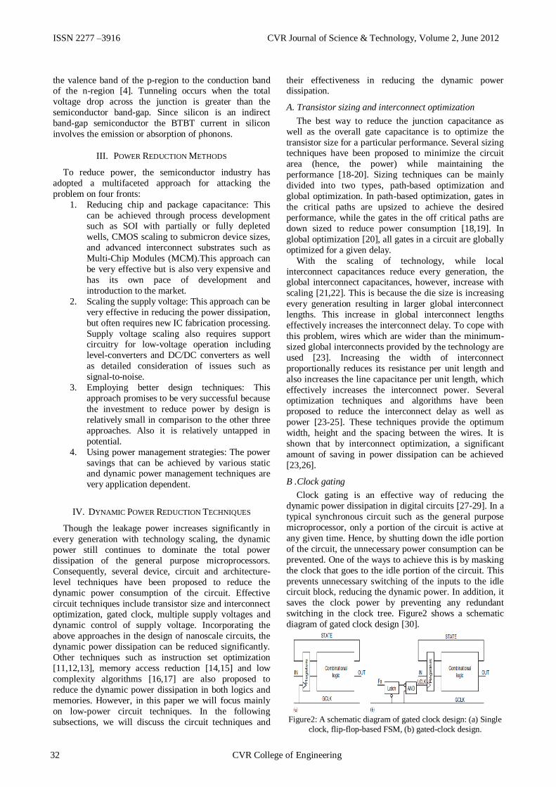
ISSN 2277 –3916 CVR Journal of Science & Technology, Volume 2, June 2012
the valence band of the p-region to the conduction band of the n-region [4]. Tunneling occurs when the total
voltage drop across the junction is greater than the
semiconductor band-gap. Since silicon is an indirect
band-gap semiconductor the BTBT current in silicon
involves the emission or absorption of phonons.
III. POWER REDUCTION METHODS
To reduce power, the semiconductor industry has
adopted a multifaceted approach for attacking the
problem on four fronts:
1. Reducing chip and package capacitance: This
can be achieved through process development such as SOI with partially or fully depleted
wells, CMOS scaling to submicron device sizes,
and advanced interconnect substrates such as
Multi-Chip Modules (MCM).This approach can
be very effective but is also very expensive and
has its own pace of development and
introduction to the market.
2. Scaling the supply voltage: This approach can be
very effective in reducing the power dissipation,
but often requires new IC fabrication processing.
Supply voltage scaling also requires support circuitry for low-voltage operation including
level-converters and DC/DC converters as well
as detailed consideration of issues such as
signal-to-noise.
3. Employing better design techniques: This
approach promises to be very successful because
the investment to reduce power by design is
relatively small in comparison to the other three
approaches. Also it is relatively untapped in
potential.
4. Using power management strategies: The power
savings that can be achieved by various static and dynamic power management techniques are
very application dependent.
IV. DYNAMIC POWER REDUCTION TECHNIQUES
Though the leakage power increases significantly in
every generation with technology scaling, the dynamic
power still continues to dominate the total power
dissipation of the general purpose microprocessors.
Consequently, several device, circuit and architecture-
level techniques have been proposed to reduce the
dynamic power consumption of the circuit. Effective
circuit techniques include transistor size and interconnect optimization, gated clock, multiple supply voltages and
dynamic control of supply voltage. Incorporating the
above approaches in the design of nanoscale circuits, the
dynamic power dissipation can be reduced significantly.
Other techniques such as instruction set optimization
[11,12,13], memory access reduction [14,15] and low
complexity algorithms [16,17] are also proposed to
reduce the dynamic power dissipation in both logics and
memories. However, in this paper we will focus mainly
on low-power circuit techniques. In the following
subsections, we will discuss the circuit techniques and
their effectiveness in reducing the dynamic power dissipation.
A. Transistor sizing and interconnect optimization
The best way to reduce the junction capacitance as
well as the overall gate capacitance is to optimize the
transistor size for a particular performance. Several sizing techniques have been proposed to minimize the circuit
area (hence, the power) while maintaining the
performance [18-20]. Sizing techniques can be mainly
divided into two types, path-based optimization and
global optimization. In path-based optimization, gates in
the critical paths are upsized to achieve the desired
performance, while the gates in the off critical paths are
down sized to reduce power consumption [18,19]. In
global optimization [20], all gates in a circuit are globally
optimized for a given delay.
With the scaling of technology, while local
interconnect capacitances reduce every generation, the global interconnect capacitances, however, increase with
scaling [21,22]. This is because the die size is increasing
every generation resulting in larger global interconnect
lengths. This increase in global interconnect lengths
effectively increases the interconnect delay. To cope with
this problem, wires which are wider than the minimum-
sized global interconnects provided by the technology are
used [23]. Increasing the width of interconnect
proportionally reduces its resistance per unit length and
also increases the line capacitance per unit length, which
effectively increases the interconnect power. Several optimization techniques and algorithms have been
proposed to reduce the interconnect delay as well as
power [23-25]. These techniques provide the optimum
width, height and the spacing between the wires. It is
shown that by interconnect optimization, a significant
amount of saving in power dissipation can be achieved
[23,26].
B .Clock gating
Clock gating is an effective way of reducing the
dynamic power dissipation in digital circuits [27-29]. In a
typical synchronous circuit such as the general purpose
microprocessor, only a portion of the circuit is active at
any given time. Hence, by shutting down the idle portion
of the circuit, the unnecessary power consumption can be
prevented. One of the ways to achieve this is by masking
the clock that goes to the idle portion of the circuit. This
prevents unnecessary switching of the inputs to the idle circuit block, reducing the dynamic power. In addition, it
saves the clock power by preventing any redundant
switching in the clock tree. Figure2 shows a schematic
diagram of gated clock design [30].
Figure2: A schematic diagram of gated clock design: (a) Single
clock, flip-flop-based FSM, (b) gated-clock design.
32 CVR College of Engineering

ISSN 2277 –3916 CVR Journal of Science & Technology, Volume 2, June 2012
The inputs to the combinational logic come through the registers, which are usually composed of sequential
elements, such as D flip-flops. A gated clock design can
be obtained by modifying the clocking structure shown in
Fig. 2(a). A control signal (fa) is used to selectively stop
the local clock (LCLK) when the combinational block is
not used. The local clock is blocked when fa is high. The
latch shown in Fig. 2(b) is necessary to prevent any
glitches in fa from propagating to the AND gate when the
global clock (GCLK) is high. The circuit operates as
follows. The signal fa is only valid before the rising edge
of the global clock. When the global clock is low, the latch is transparent, however, fa does not affect the AND
gate. If fa is high during the low-to-high transition of the
global clock, then the global clock will be blocked by the
AND gate and local clock will remain at low.
Power saving using gated clock technique strongly
depends on the efficient synthesis and optimization of
dedicated clock-stopping circuitry. Effective clock gating
requires a methodology that determines which circuits are
gated, when, and for how long. Clock-gating schemes
that either result in frequent toggling of the clock-gated
circuit between enabled and disabled states, or apply clock gating to such small blocks that the clock-gating
control circuitry is almost as large as the blocks
themselves, incur large overhead. This overhead may
result in power dissipation to be higher than that without
clock gating. There are many synthesis algorithm
proposed to efficiently cluster the circuit module for
clock gating [27-30] as well as for proper clock routing to
minimize the switching capacitance of the clock tree
[28,29].
An architecture-level technique called deterministic
clock gating (DCG) is also proposed. This technique is
based on the key observation that for many of the pipeline stages in a modern processor, a circuit block
usage in a specific cycle in the near future is
deterministically known a few cycles ahead of time.
C .Low-voltage operation
Supply voltage scaling was originally developed for
switching power reduction. It is an effective method for switching power reduction because of the quadratic
dependency of switching power on supply voltage.
Supply voltage scaling also helps reduce leakage power
since the sub-threshold leakage due to GIDL and DIBL
decreases as well as the gate leakage component when the
supply voltage is scaled down. In a 1.2 V, 0.13 mm
technology, it is shown that the supply voltage scaling
has impact in the orders of V3 and V4 on sub-threshold
leakage and gate leakage, respectively. However, since
the gate delay increases with decreasing VDD, globally
lowering VDD degrades the overall circuit performance. To achieve low-power benefits without compromising
performance, two ways of lowering supply voltage can be
employed: static and dynamic supply scaling.
(i) Static supply voltage scaling schemes: In this
technique, higher supply voltage is used in the critical
paths of the circuit, while lower supply voltages are used
in the off critical paths. Since the speed requirements of
the non-critical units are lower than the critical ones,
supply voltage of non-critical unit clusters can be lowered
without degrading system performance. The secondary voltages may be generated off-chip [31] or regulated on-
die from the core supply [32]. Depending on how many
supply voltages are available, voltage scaling may be
classified as multiple voltage approach or dual voltage
approach.
In dual/multiple supply voltage technique, whenever
an output from a low VDD cluster has to drive an input to
a high VDD cluster, a level conversion is needed at the
interface [33]. If a gate operating at a lower supply
voltage directly drives a gate operating with a higher
supply voltage, a large amount of static current is likely to flow through the PMOS transistors of the gate with
higher supply voltage. This is because when the output of
the low-voltage gate is high, its voltage level may not be
sufficient to turn-off the PMOS of the succeeding high-
voltage gate. To avoid this problem level converters are
used to convert the low-voltage output to the high-voltage
level. A typical level converter circuit is shown in Fig. 3.
[34]. While the level converter eliminates the static or
short circuit power dissipation, the power consumption
within itself may be substantial. However, this technique
is not very effective with tight timing constraints. The gate clustering problem for multiple supply voltage
operation can be simplified if level converters are used.
Several techniques have been proposed to synthesize the
circuit with dual supply voltage [34,35,37,38] considering
the power consumption and/or delay of the level
converters.
Another important issue of multiple supply voltage
design is to decide how many supply voltages are
optimum for a design and what should be the supply
voltages. Several techniques have been proposed to select
the optimal set of supply voltages taking level converters
into account [34,37]. Techniques to select the optimal low supply voltage in a dual supply design are also
proposed [39,40].
(a) (b)
Figure3: (a) Level converter circuit for interfacing gates
operating at a lower supply voltage to gates at a higher supply voltage, (b) can be used to interface low-voltage gates with
multiple fanouts with high-voltage gates.
(ii) Dynamic supply voltage scaling schemes: Dynamic
supply scaling overrides the cost of using two supply
voltages, by adapting the single supply voltage to the
performance demand. The highest supply voltage delivers
the highest performance at the fastest designed frequency
of operation. When performance demand is low, supply
voltage and clock frequency is lowered, just delivering
CVR College of Engineering 33

ISSN 2277 –3916 CVR Journal of Science & Technology, Volume 2, June 2012
the required performance with substantial power reduction [41]. There are three key components for
implementing DVS in a general-purpose processor: (1) an
operating system that can intelligently vary the processor
speed, (2) a regulation loop that can generate the
minimum voltage required for the desired speed, and (3)
a microprocessor that can operate over a wide voltage
range. Fig. 4 shows a DVS system architecture [42].
Control of the processor speed must be under software
control, as the hardware alone may not distinguish
whether the currently executing instruction is part of a
compute intensive task or a non-speed-critical task. Supply voltage is controlled by hard-wire frequency–
voltage feedback loop, using a ring oscillator as a critical
path replica. All chips operate at the same clock
frequency and same supply voltage, which are generated
from the ring oscillator and the regulator.
Figure4: Dynamic Voltage scaling architecture
V. LEAKAGE POWER REDUCTION TECHNIQUES
Since circuits are mostly designed for the highest
performance and overall system cycle time requirements,
they are composed of large gates, highly parallel
architectures with logic duplication. As such, the leakage power consumption is substantial for such circuits.
However, not every application requires a fast circuit to
operate at the highest performance level all the time.
Modules, in which computation is less e.g. functional
units in a microprocessor or sections of a cache, are often
idle. It is of interest to conceive of methods that can
reduce the leakage power consumed by these circuits.
Different circuit techniques have been proposed to reduce
leakage energy utilizing this slack without impacting
performance. Standby leakage reduction techniques put
the entire system in a low leakage mode when
computation is not required. Active leakage reduction techniques slow down the system by dynamically
changing the Vth to reduce leakage when maximum
performance is not needed. In active mode, the operating
temperature increases due to the switching activities of
transistors. This has an exponential effect on sub
threshold leakage making this the dominant leakage
component during active mode and amplifying the
leakage problem.
Design time techniques exploit the delay slack in non-
critical paths to reduce leakage. These techniques are
static; once it is fixed, it cannot be changed dynamically
while the circuit is operating. Design time techniques include, dual threshold CMOS, changing doping profile,
higher oxide thickness, higher oxide thickness.
Run time techniques include Standby leakage
reduction, natural transistor stacks, sleep transistor,
forward/reverse body biasing, active leakage reduction
techniques, dynamic Vth scaling (DVTS), circuit
techniques to reduce leakage in cache memories[5].
Many circuit techniques targeting the reduction of
leakage power have appeared in the literature. Most of
these techniques target the circuits during the standby
operation mode and some target the circuits during the active mode of operation. Also, some of these techniques
mainly aim to reduce sub-threshold leakage current while
others tend to reduce gate leakage current. We can
categorize leakage reduction circuit techniques into the
following classes:
A. Transistor stacking techniques
All these techniques are based on the fact that when
there are two or more stacked transistors which are
switched OFF. Transistor stacking has a dual effect in
reducing the sub-threshold leakage current. It increases
the source bias of upper transistors in the stack and also
lowers the gate-to-source voltages of these transistors, as
shown in Fig.5. Both of these effects result in a lower
sub-threshold leakage current.
Reducing leakage through the use of transistor stacks
depends on the choice of input pattern during standby
periods since it determines the number of OFF transistors in the stack. Leakage current dependencies on circuit
state can be exploited and used to determine a low
leakage state by using a heuristic search algorithm to find
the minimum leakage input vector, which is fed into the
circuit during sleep mode [43].
Figure5: The effect of transistor stacks in reducing Isub
The most straightforward way to find a low leakage input vector is to enumerate all combinations of primary
inputs. For a circuit with ‗n‘ primary inputs, there are
‗2n‘ combinations for input states. Due to the exponential
complexity with respect to the number of primary inputs,
such an exhaustive method is limited to circuits with a
small number of primary inputs. For large circuits, a
random search based technique can be used to find the
best input combinations. This method involves generating
a large number of primary inputs, evaluating the leakage
of each input, and keeping track of the best vector giving
the minimal leakage current. A more efficient way is to employ a genetic algorithm to exploit historical
information to speculate on new search points with
34 CVR College of Engineering
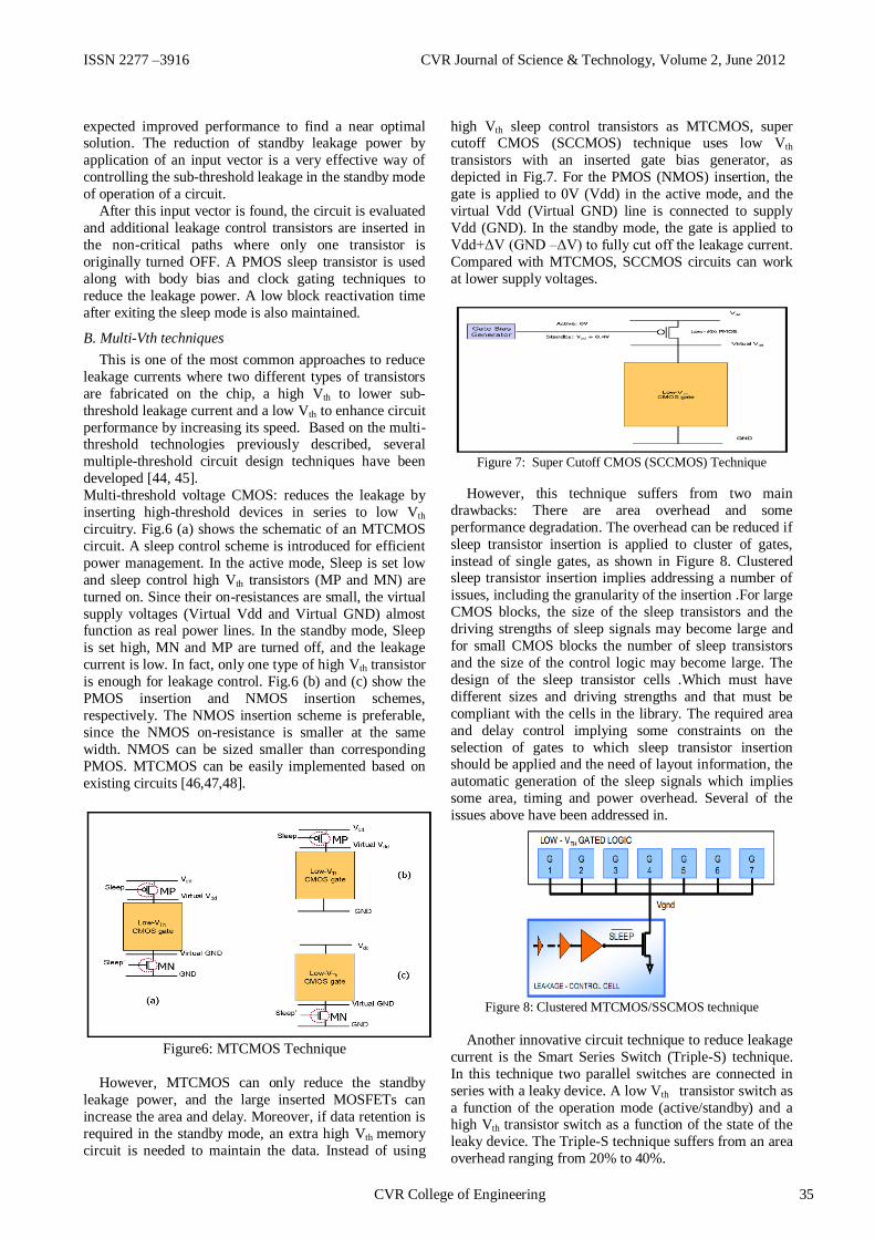
ISSN 2277 –3916 CVR Journal of Science & Technology, Volume 2, June 2012
expected improved performance to find a near optimal solution. The reduction of standby leakage power by
application of an input vector is a very effective way of
controlling the sub-threshold leakage in the standby mode
of operation of a circuit.
After this input vector is found, the circuit is evaluated
and additional leakage control transistors are inserted in
the non-critical paths where only one transistor is
originally turned OFF. A PMOS sleep transistor is used
along with body bias and clock gating techniques to
reduce the leakage power. A low block reactivation time
after exiting the sleep mode is also maintained.
B. Multi-Vth techniques
This is one of the most common approaches to reduce
leakage currents where two different types of transistors
are fabricated on the chip, a high Vth to lower sub-
threshold leakage current and a low Vth to enhance circuit
performance by increasing its speed. Based on the multi-threshold technologies previously described, several
multiple-threshold circuit design techniques have been
developed [44, 45].
Multi-threshold voltage CMOS: reduces the leakage by
inserting high-threshold devices in series to low Vth
circuitry. Fig.6 (a) shows the schematic of an MTCMOS
circuit. A sleep control scheme is introduced for efficient
power management. In the active mode, Sleep is set low
and sleep control high Vth transistors (MP and MN) are
turned on. Since their on-resistances are small, the virtual
supply voltages (Virtual Vdd and Virtual GND) almost function as real power lines. In the standby mode, Sleep
is set high, MN and MP are turned off, and the leakage
current is low. In fact, only one type of high Vth transistor
is enough for leakage control. Fig.6 (b) and (c) show the
PMOS insertion and NMOS insertion schemes,
respectively. The NMOS insertion scheme is preferable,
since the NMOS on-resistance is smaller at the same
width. NMOS can be sized smaller than corresponding
PMOS. MTCMOS can be easily implemented based on
existing circuits [46,47,48].
Figure6: MTCMOS Technique
However, MTCMOS can only reduce the standby
leakage power, and the large inserted MOSFETs can
increase the area and delay. Moreover, if data retention is
required in the standby mode, an extra high Vth memory
circuit is needed to maintain the data. Instead of using
high Vth sleep control transistors as MTCMOS, super cutoff CMOS (SCCMOS) technique uses low Vth
transistors with an inserted gate bias generator, as
depicted in Fig.7. For the PMOS (NMOS) insertion, the
gate is applied to 0V (Vdd) in the active mode, and the
virtual Vdd (Virtual GND) line is connected to supply
Vdd (GND). In the standby mode, the gate is applied to
Vdd+ΔV (GND –ΔV) to fully cut off the leakage current.
Compared with MTCMOS, SCCMOS circuits can work
at lower supply voltages.
Figure 7: Super Cutoff CMOS (SCCMOS) Technique
However, this technique suffers from two main
drawbacks: There are area overhead and some
performance degradation. The overhead can be reduced if
sleep transistor insertion is applied to cluster of gates,
instead of single gates, as shown in Figure 8. Clustered sleep transistor insertion implies addressing a number of
issues, including the granularity of the insertion .For large
CMOS blocks, the size of the sleep transistors and the
driving strengths of sleep signals may become large and
for small CMOS blocks the number of sleep transistors
and the size of the control logic may become large. The
design of the sleep transistor cells .Which must have
different sizes and driving strengths and that must be
compliant with the cells in the library. The required area
and delay control implying some constraints on the
selection of gates to which sleep transistor insertion should be applied and the need of layout information, the
automatic generation of the sleep signals which implies
some area, timing and power overhead. Several of the
issues above have been addressed in.
Figure 8: Clustered MTCMOS/SSCMOS technique
Another innovative circuit technique to reduce leakage
current is the Smart Series Switch (Triple-S) technique.
In this technique two parallel switches are connected in
series with a leaky device. A low Vth transistor switch as
a function of the operation mode (active/standby) and a high Vth transistor switch as a function of the state of the
leaky device. The Triple-S technique suffers from an area
overhead ranging from 20% to 40%.
CVR College of Engineering 35

ISSN 2277 –3916 CVR Journal of Science & Technology, Volume 2, June 2012
Dual-threshold voltage CMOS: For a logic circuit, a higher threshold voltage can be assigned to some
transistors in non-critical paths so as to reduce the
leakage current, while the performance is maintained due
to the use of low threshold transistors in the critical paths.
Therefore, no additional leakage control transistors are
required, and both high performance and low power can
be achieved simultaneously. Dual-threshold CMOS
(DTCMOS) has the same critical delay as the single low
CMOS circuit, but the transistors in non-critical paths can
be assigned high to reduce leakage power. Dual threshold
technique is good for leakage power reduction during both standby and active modes without delay and area
overhead [46].
Dynamic threshold CMOS: For dynamic threshold
CMOS (DTMOS), the threshold voltage is altered
dynamically to suit the operating state of the circuit. A
high threshold voltage in the standby mode gives low
leakage current, while a low threshold voltage allows for
higher current drives in the active mode of operation.
Dynamic threshold CMOS can be achieved by tying the
gate and body together. Fig. 9 shows the schematic of a
DTMOS inverter. DTMOS can be developed in bulk technologies by using triple wells to reduce the parasitic
components. Stronger advantages of DTMOS can be seen
in partially depleted SOI devices. The supply voltage of
DTMOS is limited by the diode built-in potential in bulk
silicon technology. The p-n diode between source and
body should be reverse biased. Hence, this technique is
only suitable for ultra-low voltage (0.6V and below)
circuits in bulk CMOS.
Figure 9: Schematic of a DTMOS inverter
Double-gate dynamic threshold SOI CMOS: The double-
gate dynamic threshold voltage (DGDT) SOI MOSFET combines the advantages of DTMOS and double-gate FD
SOI MOSFETs without any limitation on the supply
voltage. Figure 10 shows the structure of a DGDT SOI
MOSFET. A DGDT SOI MOSFET is an asymmetrical
double-gate SOI MOSFET. Back-gate oxide is thick
enough to make the threshold voltage of the back gate
larger than the supply voltage. Since the front-gate and
back-gate surface potentials are strongly coupled to each
other, the front-gate threshold voltage changes
dynamically with the back-gate voltage. Results show
that DGDT SOI MOSFETs have nearly ideal symmetric sub-threshold characteristics. Compared with symmetric
double-gate SOI CMOS, the power delay product of
DGDT SOI CMOS is smaller [45].
Figure 10: DGDT SOI MOSFET structure
C. Dynamic Vth techniques
Dynamic threshold voltage scaling is a technique for
active leakage power reduction. This scheme utilizes
dynamic adjustment of frequency through back-gate bias
control depending on the workload of a system. When the
workload decreases, less power is consumed by
increasing Vth. Two varieties of dynamic Vth scaling
(DVTS) have been proposed [46, 47].
Vth -hopping scheme: Figure 11shows the schematic
diagram of the Vth-hopping Scheme Using the control
signal (CONT), which is obtained from software, the
power control block generates select signals, Vth –low-
Enable and Vth –high-Enable, which in turn control the substrate bias for the circuit. When the controller asserts
Vth –low-Enable, Vth in the target processor reduces to Vth
–low. On the other hand, when the controller asserts Vth -
high-Enable, the target processor Vth becomes Vth –high.
CONT is controlled by software through a software
feedback loop scheme. CONT also controls the operation
frequency of the target processor. When the controller
asserts Vth –low-Enable, the frequency controller
generates fCLK, and when the controller asserts Vth –
high-Enable, the frequency controller generates, for
example, fCLK/2.
Figure11: Schematic diagram of Vth-hopping
Dynamic Vth -scaling scheme: A block diagram of the
DVTS scheme and its feedback loop is presented in
Figure 12. A clock speed scheduler, embedded in the
operating system, determines the (reference) clock
frequency at run-time. The DVTS controller adjusts the
PMOS and NMOS body bias so that the oscillator
36 CVR College of Engineering

ISSN 2277 –3916 CVR Journal of Science & Technology, Volume 2, June 2012
frequency of the voltage-controlled oscillator tracks the given reference clock frequency. The error signal, which
is the difference between the reference clock frequency
and the oscillator frequency, is fed into the feedback
controller. The continuous feedback loop also
compensates for variation in temperature and supply
voltage [48,49].
Figure 12: Schematic of DVTS hardware
D. Supply voltage scaling techniques
Supply voltage scaling was originally developed for
switching power reduction. It is an effective method for
switching power reduction because of the quadratic
dependence of the switching power on the supply voltage.
Supply voltage scaling also helps reduce leakage power, since the sub-threshold leakage due to DIBL decreases as
the supply voltage is scaled down. For a 1.2-V 0.13µm
technology, it is shown that the supply voltage scaling
has significant impacts on sub-threshold leakage and gate
leakage (reductions in the orders of V3 and V4,
respectively). To achieve low-power benefits without
compromising performance, two ways of lowering supply
voltage can be employed: Static supply scaling and
dynamic supply scaling. In static supply scaling, multiple
supply voltages are used as shown in Figure13.
Figure 13: Two-level multiple supply voltage scheme
Critical and non-critical paths or units of the design are
clustered and powered by higher and lower supply voltages, respectively. Since the speed requirements of
the non-critical units are lower than the critical ones,
supply voltage of non-critical units can be lowered
without degrading system performance. Whenever an
output from a low Vdd unit has to drive an input of a high
Vdd unit, a level conversion is needed at the interface.
The secondary voltages may be generated off-chip or
regulated on-die from the core supply.
Dynamic supply scaling overrides the cost of using two supply voltages by adapting the single supply voltage
to performance demand. The highest supply voltage
delivers the highest performance at the fastest designed
frequency of operation .When performance demand is
low, supply voltage and clock frequency is lowered,
delivering reduced performance but with substantial
power reduction.
There are three key components for implementing
dynamic voltage scaling (DVS) in a general-purpose
microprocessor. An operating system that can
intelligently determine the processor speed, a regulation loop that can generate the minimum voltage required for
the desired speed, and a microprocessor that can operate
over a wide voltage range. Figure 14 shows DVS system
architecture. Control of the processor speed must be
under software control, as the hardware alone may not
distinguish whether the currently executing instruction is
part of a compute-intensive task or a non-speed-critical
task. Supply voltage is controlled by hard-wired
frequency-voltage feedback loop, using a ring oscillator
as a replica of the critical path. All chips operate at the
same clock frequency and same supply voltage, which are generated from the ring oscillator and the regulator.
Figure14: DVS architecture
E. Input vector control techniques
The basic idea behind input vector control techniques
for leakage reduction is to force the combinational logic
of the circuit into a low-leakage state during standby
periods. This low leakage state forces the largest number
possible of transistors to be turned OFF so as to reduce
leakage and make use of multiple OFF-transistors in stacks. Leakage current can be reduced to 10 times lower
if input vector control is used. Inserting the low-leakage
input vector during standby phases is done by either
adding multiplexers or static latches at the inputs of the
circuit. Due to the added circuitry (multiplexers/latches)
switching, which consumes power, this technique is
useful for circuits with standby periods greater than some
predetermined threshold value so that the amount of
saved power outweighs the power used by the added
circuits.
Determining the best input vector that needs to be fed into the circuit depends on circuit structure, complexity,
and size. There are three main methods for selecting the
required input vector:
(1) Analyzing the circuit and looking for a good
input vector.
CVR College of Engineering 37
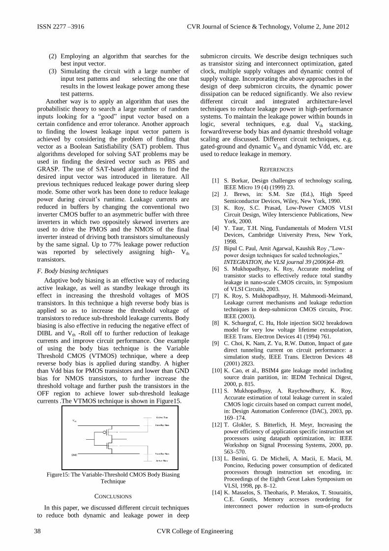
ISSN 2277 –3916 CVR Journal of Science & Technology, Volume 2, June 2012
(2) Employing an algorithm that searches for the best input vector.
(3) Simulating the circuit with a large number of
input test patterns and selecting the one that
results in the lowest leakage power among these
test patterns.
Another way is to apply an algorithm that uses the
probabilistic theory to search a large number of random
inputs looking for a ―good‖ input vector based on a
certain confidence and error tolerance. Another approach
to finding the lowest leakage input vector pattern is
achieved by considering the problem of finding that vector as a Boolean Satisfiability (SAT) problem. Thus
algorithms developed for solving SAT problems may be
used in finding the desired vector such as PBS and
GRASP. The use of SAT-based algorithms to find the
desired input vector was introduced in literature. All
previous techniques reduced leakage power during sleep
mode. Some other work has been done to reduce leakage
power during circuit‘s runtime. Leakage currents are
reduced in buffers by changing the conventional two
inverter CMOS buffer to an asymmetric buffer with three
inverters in which two oppositely skewed inverters are used to drive the PMOS and the NMOS of the final
inverter instead of driving both transistors simultaneously
by the same signal. Up to 77% leakage power reduction
was reported by selectively assigning high- Vth
transistors.
F. Body biasing techniques
Adaptive body biasing is an effective way of reducing
active leakage, as well as standby leakage through its
effect in increasing the threshold voltages of MOS
transistors. In this technique a high reverse body bias is
applied so as to increase the threshold voltage of
transistors to reduce sub-threshold leakage currents. Body
biasing is also effective in reducing the negative effect of
DIBL and Vth -Roll off to further reduction of leakage
currents and improve circuit performance. One example
of using the body bias technique is the Variable
Threshold CMOS (VTMOS) technique, where a deep
reverse body bias is applied during standby. A higher than Vdd bias for PMOS transistors and lower than GND
bias for NMOS transistors, to further increase the
threshold voltage and further push the transistors in the
OFF region to achieve lower sub-threshold leakage
currents .The VTMOS technique is shown in Figure15.
Figure15: The Variable-Threshold CMOS Body Biasing
Technique
CONCLUSIONS
In this paper, we discussed different circuit techniques
to reduce both dynamic and leakage power in deep
submicron circuits. We describe design techniques such as transistor sizing and interconnect optimization, gated
clock, multiple supply voltages and dynamic control of
supply voltage. Incorporating the above approaches in the
design of deep submicron circuits, the dynamic power
dissipation can be reduced significantly. We also review
different circuit and integrated architecture-level
techniques to reduce leakage power in high-performance
systems. To maintain the leakage power within bounds in
logic, several techniques, e.g. dual Vth stacking,
forward/reverse body bias and dynamic threshold voltage
scaling are discussed. Different circuit techniques, e.g. gated-ground and dynamic Vth and dynamic Vdd, etc. are
used to reduce leakage in memory.
REFERENCES
[1] S. Borkar, Design challenges of technology scaling, IEEE Micro 19 (4) (1999) 23.
[2] J. Brews, in: S.M. Sze (Ed.), High Speed
Semiconductor Devices, Wiley, New York, 1990. [3] K. Roy, S.C. Prasad, Low-Power CMOS VLSI
Circuit Design, Wiley Interscience Publications, New York, 2000.
[4] Y. Taur, T.H. Ning, Fundamentals of Modern VLSI Devices, Cambridge University Press, New York, 1998.
[5] Bipul C. Paul, Amit Agarwal, Kaushik Roy ,‖Low-
power design techniques for scaled technologies,‖ INTEGRATION, the VLSI journal 39 (2006)64–89.
[6] S. Mukhopadhyay, K. Roy, Accurate modeling of transistor stacks to effectively reduce total standby leakage in nano-scale CMOS circuits, in: Symposium of VLSI Circuits, 2003.
[7] K. Roy, S. Mukhopadhyay, H. Mahmoodi-Meimand, Leakage current mechanisms and leakage reduction techniques in deep-submicron CMOS circuits, Proc.
IEEE (2003). [8] K. Schuegraf, C. Hu, Hole injection SiO2 breakdown
model for very low voltage lifetime extrapolation, IEEE Trans. Electron Devices 41 (1994) 761.
[9] C. Choi, K. Nam, Z. Yu, R.W. Dutton, Impact of gate direct tunneling current on circuit performance: a simulation study, IEEE Trans. Electron Devices 48 (2001) 2823.
[10] K. Cao, et al., BSIM4 gate leakage model including source drain partition, in: IEDM Technical Digest, 2000, p. 815.
[11] S. Mukhopadhyay, A. Raychowdhury, K. Roy, Accurate estimation of total leakage current in scaled CMOS logic circuits based on compact current model, in: Design Automation Conference (DAC), 2003, pp. 169–174.
[12] T. Glokler, S. Bitterlich, H. Meyr, Increasing the power efficiency of application specific instruction set processors using datapath optimization, in: IEEE Workshop on Signal Processing Systems, 2000, pp. 563–570.
[13] L. Benini, G. De Micheli, A. Macii, E. Macii, M. Poncino, Reducing power consumption of dedicated processors through instruction set encoding, in:
Proceedings of the Eighth Great Lakes Symposium on VLSI, 1998, pp. 8–12.
[14] K. Masselos, S. Theoharis, P. Merakos, T. Stouraitis, C.E. Goutis, Memory accesses reordering for interconnect power reduction in sum-of-products
38 CVR College of Engineering

ISSN 2277 –3916 CVR Journal of Science & Technology, Volume 2, June 2012
computations, IEEE Trans. Signal Process. 50 (2002) 2889–2899.
[15] R. Saied, C. Chakrabarti, Scheduling for minimizing the number of memory accesses in low power applications, in: Workshop on VLSI Signal Processing, 1996, pp. 169–178.
[16] J. Park, W. Jeong, H. Choo, H. Mahmoodi, Y. Wang, K. Roy, High performance and low power FIR filter design based on sharing multiplication, in:
International Symposium on Low Power Electronics and Design (ISLPED‘02), 2002, pp. 295–300.
[17] D. Kang, H. Choo, K. Roy, Floorplan-aware low-complexity digital filter synthesis for low-power & high-speed, in: International Conference on Computer Design, 2004, pp. 354–357.
[18] J.P. Fishburn, A.E. Dunlop, TILOS: a posynomial programming approach to transistor sizing, IEEE
Trans. Comput. Aided Des. Integr. Circuits Syst. (1985) 326–328.
[19] [19] S. Sapatnekar, V.B. Rao, P.M. Vaidya, S.M. Kang, An exact solution of the transistor sizing problem for CMOS circuits using convex optimization, IEEE Trans. Comput. Aided Des. Integr. Circuits Syst. (1993) 1612–1634.
[20] C.P. Chen, C.C.N. Chu, D.F. Wong, Fast and exact
simulations gate and wire sizing by Lagrangian relaxation, IEEE Trans. Comput. Aided Des. Integr. Circuits Syst. 18 (1999) 1014–1025.
[21] M.T. Bohr, Interconnect scaling-the real limiter to high performance ULSI, in: International Electron Device Meeting (IEDM) Technical Digest, 1995, pp. 241–244.
[22] J.D. Meindl, Beyond Moore‘s law: the interconnect
era, Comput. Sci. Eng. (2003) 20–24. [23] M.L. Mui, K. Banerjee, A. Mehrotra, A global
interconnect optimization scheme for nanometer scale VLSI with implications for latency, bandwidth and power dissipation, IEEE Trans. Electron Devices 51 (2004) 195–203.
[24] S. Katkoori, S. Alupoaei, RT-level interconnect optimization in DSM regime, in: IEEE Computer Society Workshop on VLSI, 2000, pp. 143–148.
[25] Y. Cao, C. Hu, X. Huang, A.B. Kahng, S. Muddu, D. Stroobandt, D. Sylvester, Effects of global interconnect optimizations on performance estimation of deep submicron design, in: International Conference on Computer Aided Design, 2000, pp. 56–61.
[26] A. Naeemi, R. Venkatesan, J.D. Meindl, System-on-a-chip global interconnect optimization, in:
International SOC Conference, 2002, pp. 399–403. [27] D. Garrett, M. Stan, A. Dean, Challenges in clock
gating for a low power ASIC methodology, in: International Symposium on Low Power Electronics and Design, 1999, pp. 176–181.
[28] J. Oh, M. Pedram, Gated clock routing for low-power microprocessor design, IEEE Trans. Comput. Aided Des. Integr. Circuits Syst. 20 (2001) 715–722.
[29] N. Raghavan, V. Akella, S. Bakshi, Automatic insertion of gated clocks at register transfer level, in: International Conference on VLSI Design, 1999, pp. 48–54.
[30] L. Benini, G.D. Micheli, Automatic synthesis of low power gated clock finite state machines, IEEE Trans.
[31] Comput. Aided Des. Integr. Circuits Syst. 15 (1996) 630–643. 86 B.C. Paul et al. / INTEGRATION, the
VLSI journal 39 (2006) 64–89
[32] T. Fuse, A. Kameyama, M. Ohta, K. Ohuchi, A 0.5V power-supply scheme for low power LSIs using multi-Vt SOI CMOS technology, in: Digest of Technical Papers of Symposium on VLSI Circuits, 2001, pp. 219–220.
[33] L.R. Carley, A. Aggarwal, A completely on-chip voltage regulation technique for low power digital circuits, in: Proceedings of International Symposium on Low Power Electronics and Design, 1999, pp.
109–111. [34] Y. Kanno, H. Mizuno, K. Tanaka, T. Watanabe, Level
converters with high immunity to power-supply bouncing for high-speed sub-1-V LSIs, in: Digest of Technical Papers of Symposium on VLSI Circuits, 2000, pp. 202–203.
[35] V. Sundararajan, K.K. Parhi, Synthesis of low power CMOS VLSI circuits using dual supply voltages, in:
Design Automation Conference, 1999, pp. 72–75. [36] K. Usami, M. Horowitz, Cluster voltage scaling
techniques for low power design, in: International Symposium on Low Power Design, 1995, pp. 3–8.
[37] C. Yeh, M. Chang, S. Chang, W. Jone, Gate level design exploiting dual supply voltages for power driven applications, in: Design Automation Conference, 1999, pp. 68–71.
[38] M.C. Johnson, K. Roy, Optimal selection of supply voltages and level conversions during data path scheduling under resource constraints, in: Proceedings of the International Conference on Computer Design (ICCD), 1996, pp. 72–77.
[39] J. Chang, M. Pedram, Energy minimization using multiple supply voltages, IEEE Trans. VLSI Syst. 5 (1997) 1–8.
[40] C. Chen, A. Srivastava, M. Sarrafzadeh, On gate level power optimization using dual supply voltages, IEEE Trans. VLSI Syst. 9 (2001) 616–629.
[41] T. Kuroda, M. Hamada, Low power CMOS digital design with dual embedded adaptive power supplies, IEEE J. Solid State Circuits 35 (2000) 652–655.
[42] Jack Horgan, ―Low Power Soc Design‖, EDA Weekly Review May 17 - 21, 2004.
[43] Cadence, ―Low Power in EncounterTM RTL
Compiler‖, Product Version 5.2, December 2005. [44] Cadence, ―Low Power Application Note for RC 4.1
and SoCE 4.1 USR3‖, Version 1.0,1/14/2005. [45] V.Kursun and E. G. Friedman,Multi-Voltage CMOS
Circuit Design.New York: Wiley, 2006. [46] A. Chandrakasan and B. Brodersen, editors,‖Low
Power CMOS Design", IEEE Press, 1998. [47] J.K. Kao and A. Chandrakasan,‖Dual-Threshold
Voltage Techniques for Low-Power Digital Circuits",IEEE Journal of Solid State Circuits, Vol. 35, No. 7,pp. 1009-1018, July 2000.
[48] Liqiong Wei, Zhanping Chen, Roy, K., Yibin Ye, De, V., ―Mixed-Vth (MVT) CMOS Circuit Design Methodology for Low Power Applications‖ Design Automation Conference, 1999. Proceedings. 36th, Jun. 1999, pp. 430-435.
[49] M. Anis, S. Areibi, and M. Elmasry, ―Design and Optimization of Multithreshold CMOS(MTCMOS) Circuits,‖ IEEE Transaction on Computer-Aided Design of Integrated Circuits and Systems,vol. 22, no. 10, pp. 1324-1342, Oct. 2003.
[50] S. Sirichotiyakul and et al., ―Stand-by Power Minimization through Simultaneous Threshold Voltage Selection and Circuit Sizing,‖ Proc. of the
DAC, pp. 436-441, 1999.
CVR College of Engineering 39

ISSN 2277 –3916 CVR Journal of Science & Technology, Volume 2, June 2012
Globalized Power Aware Routing Protocols For
Mobile Ad Hoc Networks - Performance
Comparison Humaira Nishat
1 and Dr.D.Srinivasa Rao
2
1CVR College of Engineering, Department of ECE., Ibrahimpatan, R.R.District, A.P., India
Email: [email protected] 2 Jawaharlal Nehru Technological University Hyderabad, Department of ECE., Hyderabad, India
Email: [email protected]
Abstract-A mobile ad hoc network consists of nodes which
are constrained by limited battery power for their
operation. Thus, battery management is an important
issue in such networks. There are few power aware
routing protocols developed for ad hoc wireless networks
at data link, network and higher layers to solve the
problem of energy management. In this paper, we
compare the performance of two globalized power aware
routing protocols- minimum battery cost routing (MBCR)
and min-max battery cost routing (MMBCR) by
comparing the route failure times of both protocols. We
have used ns2 to carry out the simulation. From the
simulation results we observe that MMBCR have longer
network lifetime than MBCR, thus MMBCR performs
better than MBCR in a battery constraint mobile ad hoc
network environment.
Index Terms-MANETS, routing protocols, MBCR,
MMBCR, network lifetime.
I. INTRODUCTION
Mobile ad hoc network (MANET) [1] is a collection
of mobile devices called nodes that communicate with
each other over multi-hop wireless links in a
collaborative manner without the use of any centralized
infrastructure. Due to the high dynamic topology
routing protocols used in wired networks cannot be
applied to ad hoc networks. A number of routing
protocols have been proposed for ad hoc networks. Ad hoc wireless routing protocols are broadly classified
into two major categories as either proactive or table-
driven and reactive or on-demand routing protocols.
Table driven routing protocols maintains network
topology information in the form of routing tables by
periodically exchanging routing information. On the
other hand, reactive or on-demand routing protocols
obtain the necessary routing information by using a
connection establishment process.
Nodes in an ad hoc wireless network are constrained
by limited battery power and thus, energy management
[2] is an important issue in such networks. Few energy
efficient routing protocols [3] at the network layer have
been proposed in literature to solve the problem of energy management. In this paper, we study the
performance of two globalised power aware routing
protocols-MBCR & MMBCR [4] by implementing the
two routing algorithms on the same network scenario
and comparing the route failure time in each case. The
rest of the paper is organized as follows. Section two
gives a brief introduction of the two routing protocols-
MBCR & MMBCR. Section three gives the simulation
setup. Section four presents the results in the form of
performance comparison of the two routing protocols
and finally section five concludes the paper.
II. DESCRIPTION OF THE TWO ROUTING PROTOCOLS
Distributing the power consumption evenly among
nodes and minimizing the overall transmission power
are two difficult tasks in a mobile ad hoc network.
Routing algorithms described in [4], [5] attempts to find
a balance between these two factors by using node
metrics for the route selection process. The authors in
[6] proposed a power optimal scheduling and routing
protocol which tries to minimize the total average
power in the network. In [2], the authors propose a
common power protocol (COMPOW) that attempts to
satisfy three major objectives: increasing the lifetime of all the nodes, increasing the traffic-carrying capacity of
the network and reducing the contention of nodes. In
[7], authors proved that COMPOW protocols works
well only in a network with a homogeneous distribution
of nodes and exists as a special case of the
CLUSTERPOW protocol proposed by them. In [8],
authors propose a centralized algorithm that calculates
the minimum power level for each node that is required
to maintain network connectivity based on the global
information from all the nodes. The lifetime of mobile
40 CVR College of Engineering

ISSN 2277 –3916 CVR Journal of Science & Technology, Volume 2, June 2012
ad hoc networks depends mainly on each nodes battery
capacity. Hence, routing protocols must provide energy
efficient route discovery and maintenance mechanisms.
The following is a description of two globalized power aware routing protocols MBCR and MMBCR.
A. Minimum Battery Cost Routing (MBCR)
In this routing algorithm, the path containing nodes
with less remaining battery capacity is not selected and
thus the algorithm considers the summation of battery charges of all nodes while selecting the path. If the
battery cost at any instant of time t is denoted by cit,
then the remaining battery capacity of the node is given
by
fi(cit) =1/ci
t
Where f(cit) represents the battery cost function of
host ni. The higher the value of the function fi, the more
unwilling is the node to participate in the route selection
algorithm. To find a route with the maximum remaining
battery capacity, we should select a route i that has the
minimum battery cost.
Ri= min(Rj), for all jЄA Here A is the set of all routes from source to
destination. The disadvantage of MBCR is that since
only the summation of values of battery cost functions
is considered, there is a little possibility that a route
containing nodes with little remaining battery capacity
may still be selected.
B. Min-Max Battery Cost Routing (MMBCR)
In this routing algorithm, the route selection is done
based on the battery capacity of all the individual nodes
i.e., the battery of each host is used more fairly than in
the MBCR protocol. Battery cost Rj for route j is
defined as
Rj= MaxiЄroutej fi(cit)
The desired route i can be obtained from the equation
Ri=Min(Rj, jЄ A)
Where A is the set containing all possible routes. A
variant of this routing protocol minimizes the maximum cost after routing N packets to the destination or after a
time period of t seconds.
III. SIMULATION SETUP
We have used network simulator (NS 2.34) for the
simulation. NS2 [9], [10] is a discrete event driven
simulator developed at the University of Berkeley and
the Virtual Inter Network Testbed (VINT) project 1997.
We have used Fedora Version 8 as operating system.
NS2 is suitable for designing new protocols, comparing
different protocols and for traffic evaluations. It is an
object oriented simulator written in C++, with OTCL interpreter as a frontend.
The parameters used for carrying out simulation are
summarized in table1. The goal of our simulation is to
evaluate the network lifetime for both the routing
protocol MBCR and MMBCR by considering the
energy of nodes during transmission.
TABLE I.
Parameter Value
Routing Protocols MBCR & MMBCR
MAC Layer 802.11
Terrain Size 500m*500m
No. of Nodes 7
Packet Size 512B
Initial Energy 2 Joules
Simulation Time 60 sec
Traffic Source UDP
IV. SIMULATION RESULTS
We have created a network scenario of 7 nodes and
each node is assigned an initial energy of 2 joules. The simulation time was set to 60 seconds and we have used
UDP as the traffic source. There are three different
paths from source 0 to destination 4 as shown in the
figure 1. Initially, we made node 5 to transmit data to
node 1, node 2 and node 3 and thus node 5 has only 0.5
joules of energy remaining with it. To transmit data
from 0 to 4 MBCR selects the route 0-4-5 with
maximum battery capacity on an average or the
minimum total cost function. The main drawback of
this algorithm is that it does not consider the energy of
individual nodes resulting in less network lifetime even if a single node in that route dies out due to low battery
capacity. Node 5 has less battery capacity and after
certain time period it dies out resulting in route failure.
MMBCR on the other hand, considers the individual
battery capacities of each node and thus selects route 0-
1-6-4 for data transmission. In case of MMBCR, the
route containing nodes with minimum battery capacity
is avoided and route with better battery capacity of
nodes is selected resulting in delaying the route failure
time and thereby increasing the lifetime of the network.
From our simulation results we observe that the route
failure time of MBCR is much less than that of MMBCR for the same network scenario. Figure2 gives
a comparison of route failure times of MBCR and
MMBCR. The route selected for transmission of data
packets dies out at 50 seconds in case of MBCR
whereas for MMBCR the network failure time is 58.4
seconds.
CVR College of Engineering 41

ISSN 2277 –3916 CVR Journal of Science & Technology, Volume 2, June 2012
Figure 1. Screenshot showing the network scenario of seven nodes.
CONCLUSIONS
From the simulation results we conclude that when we compare the two routing protocols MBCR &
MMBCR in terms of network lifetime, MMBCR
performs better than MBCR giving more network
lifetime. The main disadvantage of MBCR is that it
does not consider the individual node energies though it
takes into account the overall battery capacity of the
route selected whereas MMBCR selects the route by
considering the individual battery capacities of each
node in that route thereby increasing the lifetime of
network.
REFERENCES
[1] B.S.Manoj and C. Siva Ram Murthy, “Ad Hoc Wireless Networks: Issues and Challenges,” Technical Report, Department of Computer Science and Engineering, Indian Institute of Technology, Madras, India, November 2003.
[2] C.F.Chiasserini and R.R.Rao, “Energy-Efficient Battery Management”, Proceedings of IEEE
INFOCOM 2000, vol.2, pp-396-403, March 2000. [3] M.Adamou and S.Sarkar, “A Framework for
Optimum Battery Management for Wireless Nodes”, Proceedings of IEEE INFOCOM 2002, pp-1783-1792, June 2002.
[4] C.K.Toh, “Maximum Battery Life Routing to Support Ubiquitous Mobile Computing in Wireless Ad Hoc Networks”, IEEE Communications
Magazine, June 2001. [5] M.Woo, S.Singh and C.S.Raghavendra, “Power-
Aware Routing in Mobile Ad Hoc Networks”, Proceedings of IEEE MOBICOM 2003, pp. 122-133, September 2003.
[6] R.L.Cruz and A.R.Santhanam, “Optimal Routing, Link Scheduling and Power Control in Multi-Hop Wireless Networks,” Proceedings of INFOCOM 2003, Vol.1 pp.702-711, April 2003.
[7] V.Kawadia, S.Narayanaswamy, R.Rozovsky, R.S.Sreenivas and P.R.Kumar, “Protocols for Media Access Control and power Control in Wireless Networks”, Proceedings of IEEE Conference on Decision and Control 2001, Vol.2, pp.1935-1940, December 2001.
[8] V.Kawadia and P.R.Kumar, “Power Control and Clustering in Ad Hoc Networks,” Proceedings of
IEEE INFOCOM 2003, Vol. 1, pp.459-469, April 2003.
[9] UCB/LBNl/VINT Network Simulator http://www.mash.cs.berkeley.edu/ns/referred on March 2010.
[10] “The Network Simulator NS-2”, available at http://www.isi.edu/nsnam/ns/referred on March 2010.
42 CVR College of Engineering

ISSN 2277 –3916 CVR Journal of Science & Technology, Volume 2, June 2012
Survey On Android OS And C2DM ServiceR.R.Dhruva
1 and V.V.N.S.Sudha
2
1CVR College of Engineering, Department of ECE., Ibrahimpatan, R.R.District, A.P., India
Email: [email protected] 2CVR College of Engineering, Department of ECE., Ibrahimpatan, R.R.District, A.P., India
Email: [email protected]
Abstract—Android is a mobile operating system for mobile
devices such as mobile tablet computers developed by Google
Inc and the Open Handset Alliance (OHA).By means of Android
Cloud to Device Messaging (C2DM) is a service developers send
data from servers to their applications on Android devices. A
simple, lightweight mechanism is provided by the service which
is used by the servers to tell mobile applications to contact the
server directly, to fetch updated application or user data. All
aspects of queuing of messages and delivery to the target
application running on the target device are handled by the
C2DM service. Using C2DM it is easy for mobile applications to
synchronize data with servers. This paper mainly surveys on the
introduction to Android OS and C2DM service.
I. INTRODUCTION
There are still several limitations for the current mobile operating systems. Some of them, like iPhone and
BlackBerry OS, are designed for and can be used only in
specific types of mobile devices [Expert users may need to
develop their own applications that require an open platform.
Closed source systems such as Windows Mobile are not
flexible enough for this purpose. Finally, another important
reason is that people want their cell phone functioning like a
PC in that whatever they can access on a desktop, they should
also be able to access on their cell phones. Therefore, an
operating system running on a cell phone should be similar to
a common desktop operating system. Symbian OS, while
having the largest market share, is not. For all above reasons, on 21 Oct 2008, Google released Android, an open source
software platform and operating system, which can run on
every mobile device, with the hope of reaching as many
mobile users as possible. Android is based on the Linux 2.6
kernel, and it provides an Android is an operating system
based on Linux with a Java programming interface. It
provides tools, e.g. a compiler, debugger and a device
emulator as well as its own Java Virtual machine (Dalvik
Virtual Machine - DVM).
Hence, standard Java bytecode cannot be run on Android.
Java Class files are converted into "dex" (Dalvik Executable) files using a tool “dx”. The applications of Android are
packed into an .apk (Android Package) file by the program
"aapt" (Android Asset Packaging Tool).To simplify
development Google provides the Android Development
Tools (ADT) for Eclipse. Automatic conversion from class to
dex files is performed by ADT and is created during
deployment. OpenGL libraries in Android support 2-D and 3-
D graphics and data storage is supported in a SQLite
database. Every Android application runs in its own process
and under its own userid which is generated automatically by
the Android system during deployment. Therefore, all the
running applications are isolated from each other and a
misbehaving application cannot easily harm other Android
applications.
II. IMPORTANT ANDROID COMPONENTS
An Android application consists out of the following parts
[4]:
Activity - Represents the presentation layer of an
Android application, e.g. a screen which is seen by
the user. There can be several activities in an
Android application and there can be switching
between those activities during runtime of the
application.
Views - The User interface of the Activities is build
with widgets classes which inherent from "android.view.View"."android.view.ViewGroups"
manages layout of rhe views.
Services - perform background tasks without
providing an UI. They can notify the user via the
notification framework in Android.
Intents are asynchronous messages which allow the
application to request functionality from other
services or activities. An application can call directly
a service or activity (explicit intent) or ask the
Android system for registered services and
applications for an intent (implicit intents). For
example the application could ask via an intent for a contact application. Application register themselves
to an intent via an IntentFilter. Intents are a powerful
concept as they allow to create loosely coupled
applications.
Broadcast Receiver - receives system messages and
implicit intents, can be used to react to changed
conditions in the system. An application can register
as a broadcast receiver for certain events and can be
started if such an event occurs.
The real-time responsiveness or latency measurement on
Android is broken down in two parts. The first part is the latency introduced in handling of an interrupt within the
Linux kernel i.e., the time it takes for the Linux kernel, after
CVR College of Engineering 43

ISSN 2277 –3916 CVR Journal of Science & Technology, Volume. 1, June 2012
receiving an interrupt (timer interrupt in our experiment), to
propagate this event to the event management layer in the
kernel. The second part is the latency introduced by Dalvik
VM, i.e., the time difference between when it receives the
event from the kernel event management layer and passes it up to the Application running on top of the VM.
III. ANDROID CLOUD TO DEVICE MESSAGING
Primary characteristics of Android Cloud to Device
Messaging are [6]:
It allows third-party application servers to send
lightweight messages to their Android applications.
The messaging service is not designed for sending a
lot of user content via the messages. Rather, it
should be used to tell the application that there is
new data on the server, so that the application can
fetch it.
There is no gurantee about delivery or the order of messages. So, for example, while you might use this
feature to tell an instant messaging application that
the user has new messages, you probably would not
use it to pass the actual messages.
There is no need for an application to run to receive
messages. When the message arrives, system wakes
up the application via Intent broadcast.
It does not provide any built-in user interface or
other handling for message data. C2DM simply
passes raw message data received straight to the
application, which has full control of how to handle it. For example, the application might post a
notification, display a custom user interface, or
silently sync data.
Android 2.2 or higher version is required that also
have the Market application installed.
It uses an existing connection for Google services.
Users are required to set up their Google account on
their mobile devices.
C2DM is basically divided into two categories:
a) Components
b) Credentials
Components are regarding the physical entities that play a
role in C2DM.Credentials are the IDs and tokens used at
different stages which ensure the authentication of parties,
and that message is going to correct place. The various
components used are Mobile Device, Third-Party Application
Server, C2DM Servers. Mobile device is the device that is
running an Android application that uses C2DM. This must
be a 2.2 Android device that has Market installed, and it must have at least one logged in Google account. Server sends data
to an Android application on the device via the C2DM server
using third party Application Server .C2DM Servers are
servers that take messages from the third-Party application
server and sends them to device. Sender ID, Application ID,
Registration ID, Google User Account, Sender Auth Token
are the various credentials used. Sender ID is an email
account associated with the application's developer. The
sender ID is used in the registration process to identify a
Android application that is permitted to send messages to the
device. This ID is typically role-based rather than being a personal account. Application ID is the application that is
registering to receive messages. The application is identified
by the package name from the manifest. This ensures that the
messages are targeted to the correct application. Registration
ID is issued by the C2DM servers to the Android application
that allows it to receive messages. Once the application has
the registration ID, it sends it to the third-party application
server, which uses it to identify each device that has
registered to receive messages for a given application. In
other words, a registration ID is tied to a particular
application for C2DM to work, the mobile device must
include at least one logged in Google account running on a particular device. ClientLogin Auth token that is saved on the
third-party application server that gives the application server
authorized access to Google services. The token is included
in the header of POST requests that send messages. For more
discussion of ClientLogin Auth tokens. The primary
processes involved in cloud-to-device messaging is:
Enabling C2DM: An Android application running
on a mobile device registers to receive messages.
Sending messages: Messages are sent by third-party
application server to the device.
Receiving messages: An Android application receives a message from a C2DM server.
A. Enabling C2DM
This is the sequence of events that occurs when an
Android application running on a mobile device registers to
receive messages:
1. The first time the application needs to use the messaging service, it fires off a registration Intent to
a C2DM server.
2. If the registration is successful, the C2DM server
broadcasts a REGISTRATION Intent which gives
application a registration ID.
3. To complete the registration, the application sends
the registration ID to the application server. The
application server typically stores the registration ID
in a database.
B. Sending the Message
For an application server to send a message, the following
things must be in place:
The application has a registration ID that allows it to
receive messages for a particular device.
The third-party application server has stored the
registration ID.
There is one more thing that needs to be in place for the application server to send messages:
ClientLoginauthorizationtoken. This is something that the
developer must have already set up on the application server
44 CVR College of Engineering

ISSN 2277 –3916 CVR Journal of Science & Technology, Volume. 1, June 2012
for the application. The ClientLogin token authorizes the
application server to send messages to a particular Android
application. An application server has one ClientLogin token
for a particular 3rd party app, and multiple registration IDs.
Each registration ID represents a particular device that has registered to use the messaging service for a particular 3rd
party app.
Here is the sequence of events that occurs when the
application server sends a message:
1. The application server sends a message to C2DM
servers.
2. Google enqueues and stores the message in case the
device is inactive.
3. When the device is online, Google sends the
message to the device.
4. On the device, the system broadcasts the message to
the specified application via Intent broadcast with proper permissions, so that only the targeted
application gets the message. This wakes the
application up. The application does not need to be
running beforehand to receive the message.
5. The application processes the message. If the
application is doing non-trivial processing, you may
want to grab a wake lock and do any processing in a
Service.
An application can unregisterC2DM if it no longer wants
to receive messages.
C. Receiving a Message
This is the sequence of events that occurs when an
Android application running on a mobile device receives a
message:
1. The system receives the incoming message and
extracts the raw key/value pairs from the message
payload. 2. The system passes the key/value pairs to the targeted
Android application in a
com.google.android.c2dm.intent.RECEIVE Intent as
a set of extras.
3. The Android application extracts the raw data from
the RECEIVE Intent by key and processes the data.
D. Writing Android Applications that Use C2DM
The various steps involved in writing the application are:
Creating the manifest.
Registering for C2DM.
Unregistering from C2DM.
Handling received data.
IV. CREATING THE MANIFEST
Every application must have an AndroidManifest.xml file
in its root directory. The manifest presents essential
information about the application to the Android system,
information the system must have before it can run any of the application's. To use the C2DM feature, the manifest must
include the following [6]:
com.google.android.c2dm.permission.RECEIVE
states that the application has permission register
and receive messages.
android.permission.INTERNET states that the application has permission to send the receiver key
to the 3rd party server.
applicationPackage + ".permission.C2D_MESSAGE
prevents other applications from registering and
receiving the application's messages.
The permision com.google.android.c2dm.SEND is
required by the receiver, so that the message can be
sent only by the C2DM framework. Both
registration and the receiving of messages are
implemented as Intents.
If the C2DM feature is critical to the application's function, android:minSdkVersion="8" should be set
in the manifest. This ensures that the application
cannot be installed in an environment in which it
could not run properly.
V. REGISTERING FOR C2DM
An Android application needs to register with C2DM
servers before receiving any message. To register it needs to
send an Intent (com.google.android.c2dm.intent.REGISTER),
with 2 extra parameters:
sender is the ID of the account authorized to send
messages to the application, typically the email
address of an account set up by the application's developer.
app is the application's ID, set with a PendingIntent
to allow the registration service to extract
application information.
Registration is not complete until the application sends the
registration ID to the third-party application server. The
application server uses the registration ID to send messages
that are targeted to the application running on that particular
device.
VI. HANDLING RECEIVED DATA
When the C2DM server receives a message from the third-party application server, C2DM extracts the raw key/value
pairs from the message payload and passes them to the
Android application in the
com.google.android.c2dm.intent.RECEIVE Intent as a set of
extras. The application extracts the data by key and processes
it, whatever that means for that application.
VII. DEVELOPING AND TESTING YOUR APPLICATIONS
Here are some guidelines for developing and testing an
Android application that uses the C2DM feature:
To develop and test your C2DM applications, you
need to run and debug the applications on an Android 2.2 system image that includes the
CVR College of Engineering 45

ISSN 2277 –3916 CVR Journal of Science & Technology, Volume. 1, June 2012
necessary underlying Google services.
To develop and debug on an actual device, you need
a device running an Android 2.2 system image that
includes the Market application.
To develop and test on the Android Emulator, you need to download the Android 2.2 version of the
Google APIs Add-On into your SDK using the
Android SDK and AVD Manager. If the C2DM
feature is critical to the application's function, be
sure to set android:minSdkVersion="8" in the
manifest. This ensures that the application cannot be
installed in an environment in which it could not run
properly.
VIII. LIMITATIONS OF C2DM:
The message size limit is 1024 bytes.
Google limits the number of messages a sender sends in aggregate, and the number of messages a
sender sends to a specific device.
CONCLUSION
Android is truly open, free development platform based on
linux and open source. Handset makers can use and
customize the platform without paying the royalty. A
component-based architecture inspired by internet mash-ups.
Parts of one application can be used in another in ways not
originally envisioned by the developer and can even replace
built-in components with own improved versions. This will
unleash a new round of creativity in the mobile space.C2DM
service is more efficient than other techniques like polling as it results in fresher data and more efficient use of network
and battery.
REFERENCES
[1] Wikipedia en.wikipedia.org/wiki/Android. [2] Google Android SDK,
http://developer.android.com/sdk/index.html.
[3] http://android-developers.blogspot.com/2010/05/android-cloud-to-device-messaging.html.
[4] http://www.vogella.de/articles/AndroidCloudToDeviceMessaging/article.html.
[5] http://blog.mediarain.com/2011/03/simple-google-android-c2dm-tutorial-push-notifications-for-android/
[6] http://code.google.com/android/c2dm/
46 CVR College of Engineering
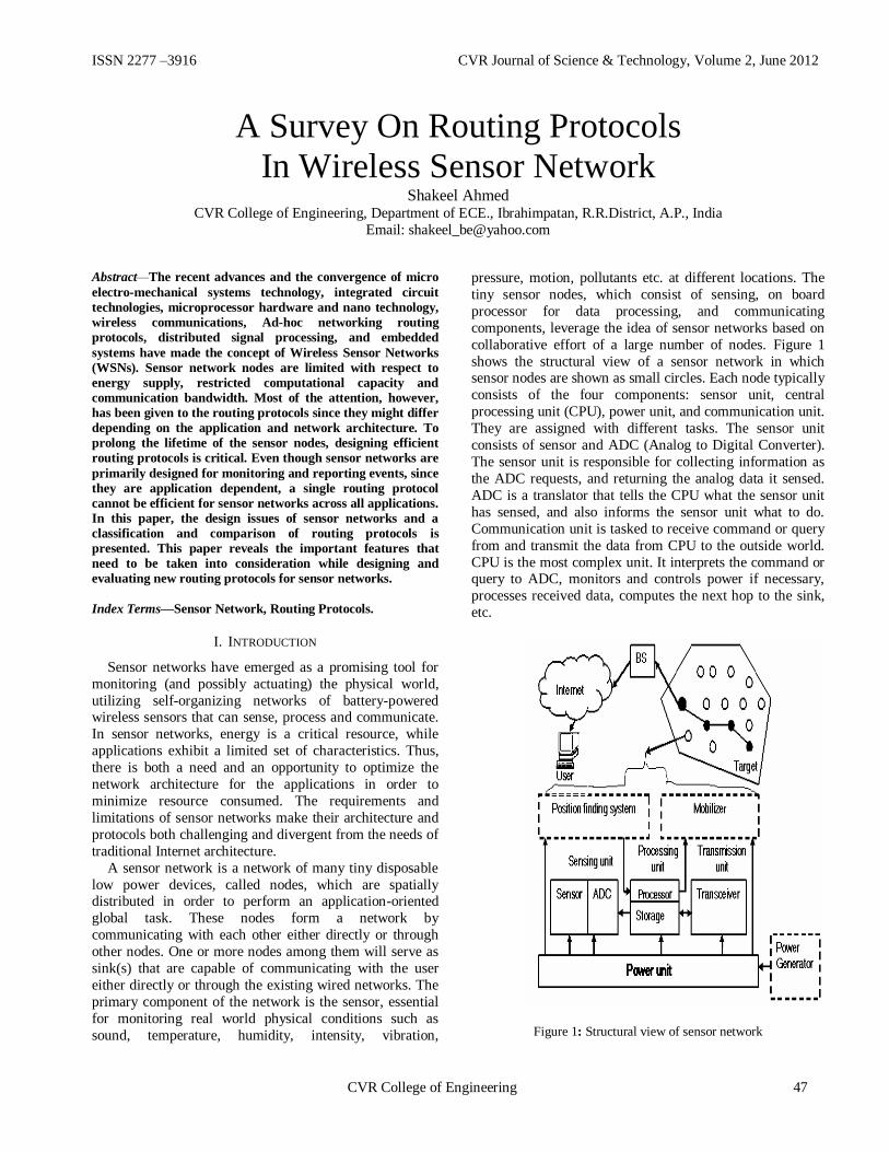
ISSN 2277 –3916 CVR Journal of Science & Technology, Volume 2, June 2012
A Survey On Routing Protocols
In Wireless Sensor Network Shakeel Ahmed
CVR College of Engineering, Department of ECE., Ibrahimpatan, R.R.District, A.P., India
Email: [email protected]
Abstract—The recent advances and the convergence of micro
electro-mechanical systems technology, integrated circuit
technologies, microprocessor hardware and nano technology,
wireless communications, Ad-hoc networking routing
protocols, distributed signal processing, and embedded
systems have made the concept of Wireless Sensor Networks
(WSNs). Sensor network nodes are limited with respect to
energy supply, restricted computational capacity and
communication bandwidth. Most of the attention, however,
has been given to the routing protocols since they might differ
depending on the application and network architecture. To
prolong the lifetime of the sensor nodes, designing efficient
routing protocols is critical. Even though sensor networks are
primarily designed for monitoring and reporting events, since
they are application dependent, a single routing protocol
cannot be efficient for sensor networks across all applications.
In this paper, the design issues of sensor networks and a
classification and comparison of routing protocols is
presented. This paper reveals the important features that
need to be taken into consideration while designing and
evaluating new routing protocols for sensor networks.
Index Terms—Sensor Network, Routing Protocols.
I. INTRODUCTION
Sensor networks have emerged as a promising tool for
monitoring (and possibly actuating) the physical world,
utilizing self-organizing networks of battery-powered wireless sensors that can sense, process and communicate.
In sensor networks, energy is a critical resource, while
applications exhibit a limited set of characteristics. Thus,
there is both a need and an opportunity to optimize the
network architecture for the applications in order to
minimize resource consumed. The requirements and
limitations of sensor networks make their architecture and
protocols both challenging and divergent from the needs of
traditional Internet architecture.
A sensor network is a network of many tiny disposable
low power devices, called nodes, which are spatially distributed in order to perform an application-oriented
global task. These nodes form a network by
communicating with each other either directly or through
other nodes. One or more nodes among them will serve as
sink(s) that are capable of communicating with the user
either directly or through the existing wired networks. The
primary component of the network is the sensor, essential
for monitoring real world physical conditions such as
sound, temperature, humidity, intensity, vibration,
pressure, motion, pollutants etc. at different locations. The
tiny sensor nodes, which consist of sensing, on board
processor for data processing, and communicating
components, leverage the idea of sensor networks based on
collaborative effort of a large number of nodes. Figure 1
shows the structural view of a sensor network in which sensor nodes are shown as small circles. Each node typically
consists of the four components: sensor unit, central
processing unit (CPU), power unit, and communication unit.
They are assigned with different tasks. The sensor unit
consists of sensor and ADC (Analog to Digital Converter).
The sensor unit is responsible for collecting information as
the ADC requests, and returning the analog data it sensed.
ADC is a translator that tells the CPU what the sensor unit
has sensed, and also informs the sensor unit what to do.
Communication unit is tasked to receive command or query
from and transmit the data from CPU to the outside world.
CPU is the most complex unit. It interprets the command or query to ADC, monitors and controls power if necessary,
processes received data, computes the next hop to the sink,
etc.
Figure 1: Structural view of sensor network
CVR College of Engineering 47

ISSN 2277 –3916 CVR Journal of Science & Technology, Volume 2, June 2012
Power unit supplies power to sensor unit, processing
unit and communication unit. Each node may also consist
of the two optional components namely Location finding
system and Mobilizer. If the user requires the knowledge
of location with high accuracy then the node should pusses Location finding system and Mobilizer may be needed to
move sensor nodes when it is required to carry out the
assigned tasks.
II. COMPARISON OF MANETS AND SENSOR NETWORKS
MANETS (Mobile Ad-hoc NETworkS) and sensor
networks are two classes of the wireless Adhoc networks
with resource constraints. MANETS typically consist of
devices that have high capabilities, mobile and operate in
coalitions. Sensor networks are typically deployed in
specific geographical regions for tracking, monitoring and
sensing. Both these wireless networks are characterized by
their ad hoc nature that lack pre deployed infrastructure for computing and communication. Both share some
characteristics like network topology is not fixed, power is
an expensive resource and nodes in the network are
connected to each other by wireless communication links.
WSNs differ in many fundamental ways from MANETS as
mentioned below.
Sensor networks are mainly used to collect
information while MANETS are designed for
distributed computing rather than information
gathering.
Sensor nodes mainly use broadcast communication paradigm whereas most
MANETS are based on point-to-point
communications.
The number of nodes in sensor networks can be
several orders of magnitude higher than that in
MANETS.
Sensor nodes may not have global identification
(ID) because of the large amount of overhead and
large number of sensors.
Sensor nodes are much cheaper than nodes in a
MANET and are usually deployed in thousands.
Sensor nodes are limited in power, computational
capacities, and memory where as nodes in a
MANET can be recharged somehow.
Usually, sensors are deployed once in their
lifetime, while nodes in MANET move really in
an Ad-hoc manner.
Sensor nodes are much more limited in their
computation and communication capabilities than
their MANET counterparts due to their low cost.
III. APPLICATIONS OF SENSOR NETWORKS
In the recent past, wireless sensor networks have found their way into a wide variety of applications and systems
with vastly varying requirements and characteristics. The
sensor networks can be used in Disaster Relief, Emergency
Rescue operation, Military, Habitat Monitoring, Health
Care, Environmental monitoring, Home networks, detecting
chemical, biological, radiological, nuclear, and explosive
material etc.
IV. CLASSIFICATION OF ROUTING PROTOCOLS
The design space for routing algorithms for WSNs is
quite large and we can classify the routing algorithms for
WSNs in many different ways. Routing protocols are
classified as
1. Node centric,
2. Data-centric, or location-aware (geo-centric) and
3. QoS based routing protocols.
Most Ad-hoc network routing protocols are node-centric
protocols where destinations are specified based on the
numerical addresses (or identifiers) of nodes. In WSNs,
node centric communication is not a commonly expected communication type. Therefore, routing protocols designed
for WSNs are more data-centric or geocentric. In data-
centric routing, the sink sends queries to certain regions and
waits for data from the sensors located in the selected
regions. Since data is being requested through queries,
attribute based naming is necessary to specify the properties
of data. Here data is usually transmitted from every sensor
node within the deployment region with significant
redundancy. In location aware routing nodes know where
they are in a geographical region. Location information can
be used to improve the performance of routing and to provide new types of services. In QoS based routing
protocols data delivery ratio, latency and energy
consumption are mainly considered. To get a good QoS
(Quality of Service), the rooting protocols must posses more
data delivery ratio, less latency and less energy
consumption.
Routing protocols can also be classified based on whether
they are reactive or proactive. A proactive protocol sets up
routing paths and states before there is a demand for routing
traffic. Paths are maintained even there is no traffic flow at
that time. In reactive routing protocol, routing actions are
triggered when there is data to be sent and disseminated to other nodes. Here paths are setup on demand when queries
are initiated.
Routing protocols are also classified based on whether
they are destination-initiated (Dst-initiated) or source-
initiated (Src-initiated). A source-initiated protocol sets up
the routing paths upon the demand of the source node, and
starting from the source node. Here source advertises the
data when available and initiates the data delivery. A
destination initiated protocol, on the other hand, initiates
path setup from a destination node.
Routing protocols are also classified based sensor network architecture. Some WSNs consist of homogenous
nodes, whereas some consist of heterogeneous nodes. Based
on this concept we can classify the protocols whether they
48 CVR College of Engineering

ISSN 2277 –3916 CVR Journal of Science & Technology, Volume 2, June 2012
are operating on a flat topology or on a hierarchical
topology. In Flat routing protocols all nodes in the network
are treated equally. When node needs to send data, it may
find a route consisting of several hops to the sink. A
hierarchical routing protocol is a natural approach to take for heterogeneous networks where some of the nodes are
more powerful than the other ones. The hierarchy does not
always depend on the power of nodes. In Hierarchical
(Clustering) protocols different nodes are grouped to form
clusters and data from nodes belonging to a single cluster
can be combined (aggregated).The clustering protocols
have several advantages like scalable, energy efficient in
finding routes and easy to manage.
V. DESIGN ISSUES OF ROUTING PROTOCOLS
Initially WSNs was mainly motivated by military
applications. Later on the civilian application domain of
wireless sensor networks have been considered, such as environmental and species monitoring, production and
healthcare, smart home etc. These WSNs may consist of
heterogeneous and mobile sensor nodes, the network
topology may be as simple as a star topology; the scale and
density of a network varies depending on the application.
To meet this general trend towards diversification, the
following important design issues of the sensor network
have to be considered.
A. Fault Tolerance
Some sensor nodes may fail or be blocked due to lack of
power, have physical damage or environmental
interference. The failure of sensor nodes should not affect
the overall task of the sensor network. This is the reliability
or fault tolerance issue. Fault tolerance is the ability to
sustain sensor network functionalities without any
interruption due to sensor node failures.
B. Scalability
The number of sensor nodes deployed in the sensing
area may be in the order of hundreds, thousands or more
and routing schemes must be scalable enough to respond to
events.
C. Production Costs
Since the sensor networks consist of a large number of
sensor nodes, the cost of a single node is very important to
justify the overall cost of the networks and hence the cost
of each sensor node has to be kept low.
D. Operating Environment
We can set up sensor network in the interior of large
machinery, at the bottom of an ocean, in a biologically or
chemically contaminated field, in a battle field beyond the
enemy lines, in a home or a large building, in a large
warehouse, attached to animals, attached to fast moving
vehicles, in forest area for habitat monitoring etc.
E. Power Consumption
Since the transmission power of a wireless radio is
proportional to distance squared or even higher order in the
presence of obstacles, multi-hop routing will consume less
energy than direct communication. However, multi-hop
routing introduces significant overhead for topology
management and medium access control. Direct routing
would perform well enough if all the nodes were very close
to the sink. Sensor nodes are equipped with limited power
source (<0.5 Ah 1.2V).Node lifetime is strongly dependent
on its battery lifetime.
F. Data Delivery Models
Data delivery models determine when the data collected
by the node has to be delivered. Depending on the
application of the sensor network, the data delivery model to
the sink can be Continuous, Event driven, Query-driven and
Hybrid. In the continuous delivery model, each sensor sends data periodically. In event-driven models, the transmission
of data is triggered when an event occurs. In query driven
models, the transmission of data is triggered when query is
generated by the sink. Some networks apply a hybrid model
using a combination of continuous, event-driven and query
driven data delivery.
G. Data Aggregation/Fusion
Since sensor nodes might generate significant redundant
data, similar packets from multiple nodes can be aggregated
so that the number of transmissions would be reduced. Data
aggregation is the combination of data from different
sources by using functions such as suppression (eliminating
duplicates), min, max and average. As computation would
be less energy consuming than communication, substantial
energy savings can be obtained through data aggregation.
This technique has been used to achieve energy efficiency
and traffic optimization in a number of routing protocols
H. Quality of Service (QoS)
The quality of service means the quality service required
by the application, it could be the length of life time, the
data reliable, energy efficiency, and location-awareness,
collaborative-processing. These factors will affect the
selection of routing protocols for a particular application. In some applications (e.g. some military applications) the data
should be delivered within a certain period of time from the
moment it is sensed.
I. Data Latency and Overhead
These are considered as the important factors that influence routing protocol design. Data aggregation and
multi-hop relays cause data latency. In addition, some
routing protocols create excessive overheads to implement
their algorithms, which are not suitable for serious energy
constrained networks.
CVR College of Engineering 49

ISSN 2277 –3916 CVR Journal of Science & Technology, Volume 2, June 2012
J. Node Deployment
Node deployment is application dependent and affects
the performance of the routing protocol. The deployment is
either deterministic or self-organizing. In deterministic
situations, the sensors are manually placed and data is
routed through pre-determined paths. However in self
organizing systems, the sensor nodes are scattered
randomly creating an infrastructure in an Ad-hoc manner.
In that infrastructure, the position of the sink or the cluster
head is also crucial in terms of energy efficiency and
performance. When the distribution of nodes is not uniform, optimal positioning of cluster head becomes a
pressing issue to enable energy efficient network operation.
VI. COMPARISON OF ROUTING PROTOCOLS
In this paper following routing protocols are compared
according their design characteristics.
SPIN: Sensor Protocols for Information via
Negotiation.
DD: Directed Diffusion
RR: Rumor Routing
GBR: Gradient Based Routing.
CADR: Constrained Anisotropic Diffusion Routing.
COUGAR
ACQUIRE: ACtive QUery forwarding In sensoR
nEtworks
LEACH: Low Energy Adaptive Clustering
Hierarchy.
TEEN & APTEEN: [Adaptive] Threshold
sensitive Energy Efficient sensor Network.
PEGASIS: The Power-Efficient GAthering in
Sensor Information Systems.
VGA: Virtual Grid Architecture Routing.
SOP: Self Organizing Protocol.
GAF: Geographic Adaptive Fidelity.
SPAN
GEAR: Geographical and Energy Aware Routing
SAR: Sequential Assignment Routing.
SPEED: A real time routing protocol.
Table I. represents Classification and Comparison of
routing protocols in WSNs. This table is based on the
survey of [1] & [2] and modified according to application
requirements.
Table I.
Classification and Comparison of routing protocols in WSNs.
CONCLUSION
WSNs have opened the doors to many applications.
WSNs are limited with respect to energy supply, restricted
computational capacity and communication bandwidth. One
of the factor which effects the performance of the WSN is
the routing protocol. Thus, designing efficient routing
protocol is critical. Its time that designers pay attention to
several parameters, one of them being QOS.
REFERENCES
[1] J. C. Castillo, T. Olivares and L. Orozco, “Routing Protocols for WSNs,” in Proc. Research Institute of Informatics, SPAIN, 2008.
[2] S. Misra et al. (eds.), Guide to Wireless Sensor Networks, Computer Communications and Networks,
[3] DOI: 10.1007/978-1-84882-218-4 4, Springer-Verlag London Limited 2009.
[4] Jamal N. Al-daraki, Ahmed E. Kamal, “Routing Techniques in WSNs,” Iowa State University, Ames, 2000.
50 CVR College of Engineering
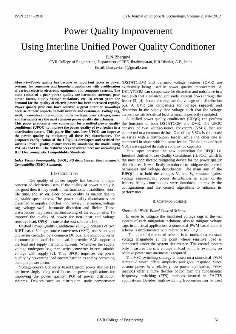
ISSN 2277 –3916 CVR Journal of Science & Technology, Volume 2, June 2012
Power Quality Improvement
Using Interline Unified Power Quality Conditioner
R.N.Bhargavi CVR College of Engineering, Department of EEE, Ibrahimpatan, R.R.District, A.P., India
Email: [email protected]
Abstract—Power quality has become an important factor in power
systems, for consumer and household appliances with proliferation
of various electric/ electronic equipment and computer systems. The
main causes of a poor power quality are harmonic currents, poor
power factor, supply voltage variations, etc. In recent years the
demand for the quality of electric power has been increased rapidly.
Power quality problems have received a great attention nowadays
because of their impacts on both utilities and customers. Voltage sag,
swell, momentary interruption, under voltages, over voltages, noise
and harmonics are the most common power quality disturbances.
This paper proposes a new connection for a unified power quality
conditioner (UPQC) to improve the power quality of two feeders in a
distribution system. This paper illustrates how UPQC can improve
the power quality by mitigating all these PQ disturbances. The
proposed configuration of the UPQC is developed and verified for
various Power Quality disturbances by simulating the model using
PSCAD/EMTDC. The disturbances considered here are according to
IEC Electromagnetic Compatibility Standards.
Index Terms- Powerquality, UPQC, PQ disturbances, Electromagnetic
Compatibility (EMC) Standards.
I. INTRODUCTION
The quality of power supply has become a major
concern of electricity users. If the quality of power supply is not good then it may result in malfunctions, instabilities, short
life time, and so on. Poor power quality is mainly due to
adjustable speed drives. The power quality disturbances are
classified as impulse, notches, momentary interruption, voltage
sag, voltage swell, harmonic distortion and flicker. These
disturbances may cause malfunctioning of the equipments. To
improve the quality of power for non-linear and voltage
sensitive load, UPQC is one of the best solutions [6].
Unified Power Quality Conditioner (UPQC) consists of two
IGBT based Voltage source converters (VSC), one shunt and
one series cascaded by a common DC bus. The shunt converter is connected in parallel to the load. It provides VAR support to
the load and supply harmonic currents. Whenever the supply
voltage undergoes sag then series converter injects suitable
voltage with supply [2]. Thus UPQC improves the power
quality by preventing load current harmonics and by correcting
the input power factor.
Voltage-Source Converter based Custom power devices [1]
are increasingly being used in custom power applications for
improving the power quality (PQ) of power distribution
systems. Devices such as distribution static compensator
(DSTATCOM) and dynamic voltage restorer (DVR) are
extensively being used in power quality improvement. A
DSTATCOM can compensate for distortion and unbalance in a
load such that a balanced sinusoidal current flows through the
feeder [3] [4]. It can also regulate the voltage of a distribution
bus. A DVR can compensate for voltage sag/swell and
distortion in the supply side voltage such that the voltage
across a sensitive/critical load terminal is perfectly regulated. A unified power-quality conditioner (UPQC) can perform
the functions of both DSTATCOM and DVR. The UPQC
consists of two voltage-source converters (VSCs) that are
connected to a common dc bus. One of the VSCs is connected
in series with a distribution feeder, while the other one is
connected in shunt with the same feeder. The dc links of both
VSCs are supplied through a common dc capacitor.
This paper presents the new connection for UPQC i.e.
Interline Unified Power Quality Conditioner (IUPQC) which is
the most sophisticated mitigating device for the power quality
disturbances. It was firstly introduced to mitigate the current harmonics and voltage disturbances. The main aim of the
IUPQC is to hold the voltages Vt1 and Vt2 constant against
voltage sag/swell/any power disturbances in either of the
feeders. Many contributions were introduced to modify the
configurations and the control algorithms to enhance its
performance.
II. CONTROL SCHEME
Sinusoidal PWM-Based Control Scheme
In order to mitigate the simulated voltage sags in the test
system of each mitigation technique, also to mitigate voltage
sags in practical application, a sinusoidal PWM-based control
scheme is implemented, with reference to IUPQC.
The aim of the control scheme is to maintain a constant
voltage magnitude at the point where sensitive load is
connected, under the system disturbance. The control system
only measures the rms voltage at load point, in example, no
reactive power measurements is required.
The VSC switching strategy is based on a sinusoidal PWM technique which offers simplicity and good response. Since
custom power is a relatively low-power application, PWM
methods offer a more flexible option than the fundamental
frequency switching (FFS) methods favored in FACTS
applications. Besides, high switching frequencies can be used
CVR College of Engineering 51
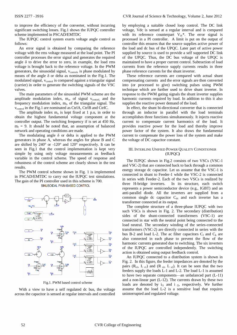
ISSN 2277 –3916 CVR Journal of Science & Technology, Volume 2, June 2012
to improve the efficiency of the converter, without incurring
significant switching losses. Fig.1 shows the IUPQC controller
scheme implemented in PSCAD/EMTDC
The IUPQC control system exerts voltage angle control as follows:
An error signal is obtained by comparing the reference
voltage with the rms voltage measured at the load point. The PI
controller processes the error signal and generates the required
angle δ to drive the error to zero, in example, the load rms
voltage is brought back to the reference voltage. In the PWM
generators, the sinusoidal signal, vcontrol, is phase modulated by
means of the angle δ or delta as nominated in the Fig.1. The
modulated signal, vcontrol is compared against a triangular signal
(carrier) in order to generate the switching signals of the VSC
valves.
The main parameters of the sinusoidal PWM scheme are the amplitude modulation index, ma, of signal vcontrol, and the
frequency modulation index, mf, of the triangular signal. The
vcontrol in the Fig.1 are nominated as CtrlA, CtrlB and CtrlC.
The amplitude index ma is kept fixed at 1 p.u, in order to
obtain the highest fundamental voltage component at the
controller output. The switching frequency if is set at 450 Hz,
mf = 9. It should be noted that, an assumption of balanced
network and operating conditions are made.
The modulating angle δ or delta is applied to the PWM
generators in phase A, whereas the angles for phase B and C
are shifted by 240° or -120° and 120° respectively. It can be seen in Fig.1 that the control implementation is kept very
simple by using only voltage measurements as feedback
variable in the control scheme. The speed of response and
robustness of the control scheme are clearly shown in the test
results.
The PWM control scheme shown in Fig. 1 is implemented
in PSCAD/EMTDC to carry out the IUPQC test simulations.
The gain of the PI controller used in this scheme is 700.
Fig.1. PWM based control scheme
With a view to have a self regulated dc bus, the voltage
across the capacitor is sensed at regular intervals and controlled
by employing a suitable closed loop control. The DC link
voltage, Vdc is sensed at a regular interval and is compared
with its reference counterpart Vdc*. The error signal is
processed in a PI controller. A limit is put on the output of controller this ensures that the source supplies active power of
the load and dc bus of the UPQC. Later part of active power
supplied by source is used to provide a self supported DC link
of the UPQC. Thus, the DC bus voltage of the UPQC is
maintained to have a proper current control. Subtraction of load
currents from the reference supply currents results in three
phase reference currents for the shunt inverter.
These reference currents are compared with actual shunt
compensating currents and the error signals are then converted
into (or processed to give) switching pulses using PWM
technique which are further used to drive shunt inverter. In
response to the PWM gating signals the shunt inverter supplies harmonic currents required by load. In addition to this it also
supplies the reactive power demand of the load.
In effect, the shunt bi-directional converter that is connected
through an inductor in parallel with the load terminals
accomplishes three functions simultaneously. It injects reactive
current to compensate current harmonics of the load. It
provides reactive power for the load and thereby improve
power factor of the system. It also draws the fundamental
current to compensate the power loss of the system and make
the voltage of DC capacitor constant.
III. INTERLINE UNIFIED POWER QUALITY CONDITIONER
(IUPQC)
The IUPQC shown in Fig.2 consists of two VSCs (VSC-1
and VSC-2) that are connected back to back through a common
energy storage dc capacitor. Let us assume that the VSC-1 is
connected in shunt to Feeder-1 while the VSC-2 is connected
in series with Feeder-2. Each of the two VSCs is realized by
three H-bridge inverters. In its structure, each switch
represents a power semiconductor device (e.g., IGBT) and an
anti-parallel diode. All the inverters are supplied from a
common single dc capacitor Cdc and each inverter has a
transformer connected at its output.
The complete structure of a three-phase IUPQC with two such VSCs is shown in Fig. 2. The secondary (distribution)
sides of the shunt-connected transformers (VSC-1) are
connected in star with the neutral point being connected to the
load neutral. The secondary winding of the series-connected
transformers (VSC-2) are directly connected in series with the
bus B-2 and load L-2. The ac filter capacitors Cf and Ck are
also connected in each phase to prevent the flow of the
harmonic currents generated due to switching. The six inverters
of the IUPQC are controlled independently. The switching
action is obtained using output feedback control.
An IUPQC connected to a distribution system is shown in Fig. 2. In this figure, the feeder impedances are denoted by the
pairs (Rs1, L s1) and (R s2, L s2). It can be seen that the two
feeders supply the loads L-1 and L-2. The load L-1 is assumed
to have two separate components—an unbalanced part (L-11)
and a non-linear part (L-12). The currents drawn by these two
loads are denoted by il1 and i l2, respectively. We further
assume that the load L-2 is a sensitive load that requires
uninterrupted and regulated voltage.
52 CVR College of Engineering

ISSN 2277 –3916 CVR Journal of Science & Technology, Volume 2, June 2012
The shunt VSC (VSC-1) is connected to bus B-1 at the end
of Feeder-1, while the series VSC (VSC-2) is connected at bus
B-2 at the end of Feeder-2. The voltages of buses B-1 and B-2
and across the sensitive load terminal are denoted by Vt1, V t2, and Vl2, respectively.
Figure 2. Typical IUPQC connected in a distribution system
The aim of the IUPQC is two-fold:
To protect the sensitive load L-2 from the
disturbances occurring in the system by regulating the
voltage Vl2;
To regulate the bus B-1 voltage Vt1 against sag/swell
and or disturbances in the system.
In order to attain these aims, the shunt VSC-1 is operated as
a voltage controller while the series VSC-2 regulates the
voltage across the sensitive load. The length of Feeder-1 is
arbitrarily chosen to be twice that of Feeder-2.
The system with the below mentioned parameters is
implemented using PSCAD/ EMTDC and is analyzed for various PQ disturbances. One of the VSCs is connected in
series with a distribution feeder, while the other one is
connected in shunt with the same feeder. The dc links of both
VSCs are supplied through a common dc capacitor.
The shunt VSC (VSC-1) holds the voltage of bus B-1
constant. This is accomplished by making VSC-1 to track to a
reference voltage across the filter capacitor Cf. It is assumed
that the dc capacitor is initially charged and both the feeders
along with the IUPQC are connected at time zero. Once the
three-phase B-1 voltages become balanced, the currents drawn
by Feeder-1 also become balanced. The load L-2 bus voltages are also perfectly sinusoidal with the desired peak as the
converter VSC-2 injects the required voltages in the system.
The bus B-2 voltages will have a much smaller magnitude.
A 3-phase supply voltage of 11kv line to line, 50Hz with sag
of 81% at source end, non-linear and unbalanced load at load
end is considered. Non-linear load (Diode Rectifier feeding an
RL load) injects current harmonics into the system. IUPQC is
able to reduce the harmonics from entering into the system
using shunt control. IUPQC with its series voltage control
calculates the required voltage to be injected in series with the
line to compensate the voltage sag in the insertion transformer
produces the series injected (compensated) voltage by drawing
the required power from the DC link. IUPQC with shunt PI
controller estimates the required current to be injected in shunt
with the line to compensate the disturbances.
IV. POWER QUALITY IMPROVEMENT USING IUPQC
There are three ways to solve the problems of power quality
and provide quality power customized to meet user’s
requirement:
System improvement
Use mitigation equipment based on power electronics
Improvement of equipment immunity
Of these, the best way to handle power quality problems is
to mitigate the effects of distorted voltage or current at the
point of common coupling. This would ensure that the
harmonics are restricted from entering the distribution system and contaminating the system power as a whole. Thereby, the
other loads connected to the system are provided with clean
power. This paper illustrates how various power quality
disturbances are mitigated using equipment called IUPQC.
With UPQC Without UPQC
Figure 3. Simulation results – Comparison of Waveforms for a voltage sag of 81% with and without UPQC
(a) rms load voltage (pu)
(b) Instantaneous load voltages (kV)
(c) Instantaneous load currents (kA)
(d) Load and source active powers (MW)
(e) Load and source reactive power (MVAR)
1.Mitigation of Voltage SAG
A 3-phase supply voltage (11kv, 50Hz) with impulsive sag of 0.5 p.u magnitude and the duration about 0.5 to 30 cycles is
taken. With the system operating in the steady state, 15 cycle
impulsive voltage sag of 0.5 p.u magnitude is occurring at 0.3
msec for which the peak of the supply voltage reduces from its
CVR College of Engineering 53

ISSN 2277 –3916 CVR Journal of Science & Technology, Volume 2, June 2012
nominal value of 10kv to 5kv. The simulation results are
shown in Fig.4. The Total Harmonic Distortion (THD) at load
side is found to be 0.95%. The source voltage THD is
effectively found to be 0.045%. In order to supply the balanced power required to the load,
the DC capacitor voltage drops as soon as the sag occurs. As
the sag is removed the capacitor voltage returns to the steady
state. The voltage injected by UPQC in kV is shown in Fig.
4(d). Active and reactive powers both on source and load sides
are shown in Fig. 4 (e) and Fig. 4(f).
Figure 4. Simulation results- Mitigation of voltage sag (impulsive) Using IUPQC
(a) Instantaneous source voltage (kV)
(b) Instantaneous load voltage (kV)
(c) Three phase load and source r.m.s voltage
(d) Voltage injected by UPQC (kV)
(e) Load current (KA)
(f) Source and load active powers (MW)
(g) Source and load reactive powers (MVAR).
2. Mitigation of Voltage Swell
A 3-phase supply voltage (11kv, 50Hz) with momentary
swell of 0.26 pu magnitude and the duration about 0.5 to 30
cycles is taken. With the system operating in the steady state, a
21 cycle momentary voltage swell of 0.26 p.u magnitude is
occurring at 0.3 msec for which the peak of the supply voltage
raises from its nominal value of 10kv to 12.6kV. In order to
supply the balanced power required to the load, the DC
capacitor voltage raises as soon as the swell occurs. As the
swell is removed the capacitor voltage returns to the steady state. The Total Harmonic Distortion (THD) at load side is
found to be 1.71%. The source voltage THD is effectively
found to be 0.045%.
CONCLUSIONS
The Sinusoidal Pulse Width Modulation based control
scheme for the proposed IUPQC has been described. The
control scheme for IUPQC with shunt (PI) controller and series voltage controller has been developed.
Fig.5. Simulation results- Mitigation of a voltage swell (momentary)
(a) Instantaneous source voltage (kV)
(b) Instantaneous load voltage (kV)
(c) 3-Ф load and source r.m.s voltage (pu)
(d) Voltage injected by UPQC (kV)
(e) Load current (kA)
(f) Source and load active powers (MW)
(g) Source and load reactive powers (MVAR)
(h) Harmonic analysis at load during fault (%)
The IUPQC can mitigate various power quality disturbances
like sag, swell, momentary interruption, over voltages, under
voltages, harmonics, noise, etc. The IUPQC discussed in this
project is capable of handling system in which the loads are unbalanced and distorted.
It has been observed that an IUPQC is able to protect the
distribution system from various disturbances occurring either
in Feeder-1 or in Feeder-2. As far as the common dc link
voltage Vdc is at the reasonable level, the device works
satisfactorily. The angle controller ensures that the real power
is drawn from Feeder-1 to hold the dc link voltage constant.
Therefore, even for voltage sag or a fault in Feeder-2, VSC-1
passes real power through the dc capacitor onto VSC-2 to
regulate the load voltage.
The simulated results shows that PI controller of the shunt filter (current control mode), series filter (voltage control
mode) compensates of all types of interruptions in the load
current and source voltage, so as to maintain sinusoidal voltage
and current at load side. The series filter was tested with
different types of interruptions. The simulated results show that
54 CVR College of Engineering

ISSN 2277 –3916 CVR Journal of Science & Technology, Volume 2, June 2012
in all the stages of circuit operation, the feeder-2 load voltages
and load currents are restored close to ideal supply.
For all the types of disturbances (interruptions) the Total
Harmonic Distortion (THD) after compensation is to be less than 5% which is as per IEEE standards.
REFERENCES
[1] A. Ghosh and G. Ledwich, Power Quality Enhancement Using Custom Power Devices. Norwell, MA: Kluwer, 2002.
[2] F. Z. Peng and J. S. Lai, ―Generalized instantaneous reactive power theory for three-phase power systems,‖ IEEE Trans. Instrum. Meas., vol. 45, no. 1, pp. 293–297, Feb. 1996.
[3] G. Ledwich and A. Ghosh, ―A flexible DSTATCOM operating in voltage and current control mode,‖ Proc. Inst. Elect. Eng., Gen., Transm. Distrib., vol. 149, no. 2, pp. 215–224, 2002.
[4] M. K. Mishra, A. Ghosh, and A. Joshi, ―Operation of a
DSTATCOM in voltage control mode,‖ IEEE Trans. Power Del., vol. 18, no. 1, pp.258–264, Jan. 2003.
[5] A. Ghosh, A. K. Jindal, and A. Joshi, ―A unified power quality conditioner for voltage regulation of critical load bus,‖ in Proc. IEEE Power Eng. Soc. General Meeting, Denver, CO, Jun. 6–10, 2004.
[6] A. Ghosh and G. Ledwich, ―A unified power quality conditioner (UPQC) for simultaneous voltage and current compensation,‖ Elect Power Syst. Res., vol. 59, no. 1, pp.
55–63, 2001. [7] Understanding Power Quality Problems ,Voltage Sags and
Interruptions by Math.HJ .Bollen.
[8] Electrical Power Systems Quality, Second Edition, by Roger C. Dugan/ Mark F. Mc Granaghan, Surya Santoso/ H. Wayne Beaty.
CVR College of Engineering 55

ISSN 2277 –3916 CVR Journal of Science & Technology, Volume 2, June 2012
Power System Transient Stability Analysis
With SSSC Controller P.Nagaraju Mandadi
1 and Dr. K.Dhanvanthri
2
1CVR College of Engineering, Department of EEE., Ibrahimpatan, R.R.District, A.P., India
Email: [email protected] 2CVR College of Engineering, Department of EEE., Ibrahimpatan, R.R.District, A.P., India
E-mail: [email protected]
Abstract--The SSSC FACTS controller is applied to
a multi--machines power system for analysis of
Transient stability during faults under different
fault clearing times using MATLAB / SIMULINK
setups developed in this work. The developed
SIMULINK setup is a very general approach
showing clearly the effects of change of any
parameter on the Transient stability of a power
system. The oscillations in the power system has
been shown to get damped out very effectively by
SSSC controller and in this method of analysis, it
has been shown that a desired Transient response
can be obtained very easily and quickly with the
use of the developed SIMULINK setup on any
power system .
Index Terms--SSSC, damping, Transient stability,
Simulink, MATLAB and FACTS.
Nomenclature:
-Generator rotor angle
- Generator rotor speed
E - Magnitude of the internal voltage
V -Infinite bus voltage
H -Inertia constant in Sec
X d1 -Generator transient reactance
XL - Line reactance
P e - Electrical power output in p.u
P m - Mechanical power input in p.u
V S - Controllable voltage provided by SSSC.
- Angle of line current.
S -Angle of SSSC voltage.
Yb f -Reduced system Admittance value before
fault. Yd f -Reduced system admittance value during
fault.
Ya f -Reduced system admittance value after fault
clearance.
I. INTRODUCTION
One of the major problems in power system
has been its stability which is defined as its
ability to supply electrical power under
disturbances. If the disturbance is small, it is
known as ‘steady state stability’ whereas if it is
large and sudden, it is called ‘Transient
Stability’. In addition to this, if there occurs a
fault, it is more involved because there will be
network changes during and after fault clearance.
In Transient stability analysis, the total system is
reduced to only the number of generators and the
electrical powers from each of the generators are
calculated both during and after the fault
clearance1.
The Transient stability can be determined
solving the non-linear swing equation using any
of the available numerical methods using
MATLAB. In this process, SIMULINK setup is used which is accurate, fast, easy and reliable.
Also the effects of variation of any of the system
parameters can be quickly obtained either in
terms of numerical values or in terms of Graphs.
These graphs can be easily obtained using the
facilities available in MATLAB. Because of the
above mentioned advantages, SIMULINK setup
only is used for the entire analysis of the
problem involved in this work.
During Transient stability problem, it is a fact
that the system is subjected to oscillations and these have to be damped within a given time. To
achieve damping, ‘Power System Stabilizers’ are
used but to get the required effect from this, it
is essential that it has to be designed properly.
The development of recent FACTS(Flexible AC
Transmission System) devices such as
STATCOM, SVC, TCSC,SSSC(Static
Synchronous Series Compensator) etc are being
used for getting fast and effective control for
damping mechanical oscillations.2
This paper analyzes Transient stability of
Multi-Machine Power System. The Multi-Machine power system considered in this paper
is the standard 3 Machine 9 Bus System1
considering fault and its clearance and the effect
of SSSC is observed using the developed
Simulink setup. The method suggested and the
Simulink link setups developed can be applied to
any power system. This is mainly because of the
accuracy and correctness of the Simulink setups.
56 CVR College of Engineering

ISSN 2277 –3916 CVR Journal of Science & Technology, Volume 2, June 2012
II. ANALYSIS OF SSSC (STATIC SYNCHRONOUS
SERIES COMPENSATOR):
The SSSC is a solid-state voltage source
inverter connected in series to power
transmission lines3. It can vary the effective impedance of a transmission line such that it can
influence the power flow by injecting a
controllable voltage VS. This injected voltage
will be in quadrature with the line current and
emulates an Inductive or Capacitive reactance.
For the SSSC, the only controllable parameter is
the magnitude of VS. It is also to be mentioned
that VS changes only the current magnitude and
not its angle.
In the case of SSSC, the current is given by
I S =jX
VVE S
SV is kept in quadrature with the line current
and is given as
SV = VS Sje
When VS lags the line current by 900, the
SSSC behaves like a capacitive reactance.
The angle can be expressed as
)
The electrical power is given by
Pe = X
EVsin +
X
VVScos (1)
The term cos is given by
cos2
sin
22 EVVE
E
Equation (1) combined with above and Pe can
be written as
Pe = (X
EVsin ) ( 1 + )
Where
cos222 EVVE
VS
Rotor speed deviation is taken as control
signal. VS is dynamically related to and must
satisfy
VS = k1 ;
-VS maxmaxSS VV
and k1 is a positive gain.
III. POWER SYSTEMS CONSIDERED FOR
ANALYSIS.
The concepts developed with regards to SSSC
controller is applied to the standard (Western System Coordinated Council) WSCC 3 Machine
9 Bus system 1 as shown in Figure 1.
Figure 1. WSCC 3- Machine, 9 Bus System: All
Impedances are in P.U on a 100 MVA base
The SIMULINK setup for analyzing WSCC 3
Machine 9 BUS system with fault and without
SSSC controller is given in Figure 2.
CVR College of Engineering 57

ISSN 2277 –3916 CVR Journal of Science & Technology, Volume 2, June 2012
d1
VS1
Pe1
d1
Vs2
d2
Pe2
d2
d3
d3
d2
d1
d3
d1
d21
d31
Vs3
Pe3
Pe1
Pe2
Pe3
d21,d31
d31
To Workspace3
d21
To Workspace2
t
To Workspace
Switch2
Switch1
Switch
Pe3
W3
d3
Subsystem3
Pe2
W2
d2
Subsystem2
Pe1
W1
d1
Subsystem1
180/pi
Rad to deg1
180/pi
Rad to deg
f(u)
Pe3 POST FAULT
f(u)
Pe3 FAULT
f(u)
Pe2 POST FAULT
f(u)
Pe2 FAULT
f(u)
Pe1 POST FAULT
f(u)
Pe1 FAULT
f(u)
Net Pe3
f(u)
Net Pe2
f(u)
Net Pe1
Mux
Mux
Mux
Mux
Mux
0
K3
0
K2
0
K1
1.017
E3
1.0502
E2
1.0566
E1
Clock3
Clock2
Clock1
Clock
Figure 2. Transient Stability Analysis of 9 Bus, 3 M/C Power System Analysis without SSSC Controller, Fault at Bus 6, Line 6-9 removed.
58 CVR College of Engineering

ISSN 2277 –3916 CVR Journal of Science & Technology, Volume 2, June 2012
d1
VS1
Pe1
d1
Vs2
d2
Pe2
d2
d3
d3
d2
d1
d3
d1
d21
d31
Vs3
Pe3
Pe1
Pe2
Pe3
d21,d31
d31
To Workspace3
d21
To Workspace2
t
To Workspace
Switch2
Switch1
Switch
Pe3
W3
d3
Subsystem3
Pe2
W2
d2
Subsystem2
Pe1
W1
d1
Subsystem1
180/pi
Rad to deg1
180/pi
Rad to deg
f(u)
Pe3 POST FAULT
f(u)
Pe3 FAULT
f(u)
Pe2 POST FAULT
f(u)
Pe2 FAULT
f(u)
Pe1 POST FAULT
f(u)
Pe1 FAULT
f(u)
Net Pe3
f(u)
Net Pe2
f(u)
Net Pe1
Mux
Mux
Mux
Mux
Mux
0.2
K3
0.2
K2
0.2
K1
1.017
E3
1.0502
E2
1.0566
E1
Clock3
Clock2
Clock1
Clock
0 0.1 0.2 0.3 0.4 0.5 0.6 0.7 0.8 0.9 110
15
20
25
30
35
40
time(s)
d21,d
31(d
eg)
The swing curve with fault and without SSSC
is shown in Figure 3.
Figure 3.
The Simulink setup with SSSC controller is shown in Figure 4.
Figure 4.
CVR College of Engineering 59

ISSN 2277 –3916 CVR Journal of Science & Technology, Volume 2, June 2012
The swing curve with fault and with SSSC
controller is shown below.
From the above Figure, it is observed that the oscillations in rotor angle are completely
damped. Also, the desired transient response can
be obtained by suitably changing the parameters
using the Simulink setup of fig 4. The stability of
the system with fault can also be improved by
merely changing the parameters.
CONCLUSION
In this paper, the advantages of using SSSC
controller for obtaining sufficient damping of
oscillations for WSCC 3 Machine 9 Bus system
under fault conditions have been clearly demonstrated with the help of the developed
SIMULINK setups and the graphs. These setups
are very general and easy for implementation and
desired time responses can be quickly and
accurately obtained. Also, any SMIB and Multi-
Machine systems can be analyzed getting the
indicated advantages.
ACKNOWLEDEMENT
The authors wish to thank the management of
CVR College of Engineering for their
encouragement in the completion of this work.
REFERENCES
[1] Ramnarayan Patel, T.S.Bhatti and
D.P.Kothari, Matlab/Simulink –based
Transient Stability analysis of a multi-
machine power system, International journal
of Electrical Engineering Education 39/4.
[2] M.H. Haque, Damping improvement by
FACTS devices: A comparison between
STATCOM and SSSC,Electric Power System
Research, Vol.76,2006, pp. 865-872.
[3] Amara SAIDI,Hsan HADJ ABDALLAH,
Improvement of Transient Stability by
FACTS devices,ICGST-ACSE Journal,Vol
11 ,issue 1,June 2011.
[4] Hadi Saadat, Power System analysis
(McGraw-Hill, New York, 1999.)
[5] R. Ramanujam, Power System Dynamics-
Analysis and Simulation, PHI Learning Pvt
Ltd, 2009.
[6] P.M. Anderson and A.A. Fouad, Power
system Control and Stability.
[7] P.Kundur, Power System Stability and
Control, EPRI Power System Engineering
Series (Mc.Graw –Hill, New York, 1994).
[8] Simulink User’s Guide (The Mathworks,
Natick, MA.1999).
0 1 2 3 4 5 617
18
19
20
21
22
23
24
25
26
27
time(s)
d21,d
31(d
eg)
60 CVR College of Engineering
ISSN 2277 –3916 CVR Journal of Science & Technology, Volume 2, June 2012
Control Of Process Variables For Remote
Applications Using Lab VIEW And Internet S.Harivardhagini
1 and S.Pranavanand
2
1CVR College of Engineering, Department of EIE., Ibrahimpatan, R.R.District, A.P., India
Email:[email protected] 2VNR Vignana Jyothi Institute of Engineering & Technology, R.R.District, A.P., India
Email:[email protected]
Abstract-The paper presents a system that monitors and
controls process variables for remote applications.
LabVIEW (short for Laboratory Virtual Instrumentation
Engineering Workbench) is a visual programming
language commonly used for Data Acquisition (DAQ) and
control. LabVIEW contains a user interface, known as
front panel objects. By this we can access the acquired
process variables over the internet. The accessed process
variables like temperature, pressure, strain or any other
can be suitably conditioned and feedback for control of
the process via the internet for control. The system would
find wide application in processes which are hazardous in
nature. People can be safeguarded from hazardous effect,
in dangerous areas like chlorine industry or at places
where person gets affected by dangerous gases. This note
presents one such idea using LabVIEW and Internet.
Index Terms—LabVIEW, Process variables, PID control
Graphical system design, strain measurement, compact field point.
I. INTRODUCTION
Modern process variable measurement (level,
temperature, strain) is truly sophisticated. Standard laboratories around the world routinely measure process
variables (temperature, strain, energy, etc.,) to one
thousand of a unit. This can even be done automatically
with computer controlled equipment. The methods of
process variable measurement have changed rapidly in
recent years. Inexpensive commercial equipment for
measurement and control often will indicate
measurement to one tenth of a unit. Because of adverse
environments, sensors or instrument instability,
vibration, electrical noise, or design comprises, the
instruments may have errors whose magnitude may
vary over a large scale. It is therefore required to understand the entire process before any valuable
measurement is recorded.
The concept of measurement of process variables
like level, temperature and strain might have originated
long back and even still innovation is on for this field of
science.
In physics, temperature is a physical property of a
system that underlines the common notions of hot and
cold. Temperature is one of the principal parameters of
thermo dynamics. On the macroscopic scale,
temperature is the unique physical property that
determines the direction of heat flow between two
objects placed in thermal contact. If no heat flow
occurs, the two objects have the same temperature;
otherwise heat flows from the hotter object to the colder
object. On the microscopic scale, temperature can be
defined as the average energy in each degree of
freedom in the particles in a system. For a solid, this energy is found in the vibrations of its atoms about their
equilibrium positions.
The level can be measured using capacitive
transducer. The capacitive transducer or sensor is
nothing but the capacitor with variable capacitance. The
capacitive transducer comprises of two parallel metal
plates that are separated by the material such as air,
which is called as the dielectric material. In the typical
capacitor the distance between the two plates is fixed,
but in variable capacitance transducers the distance
between the two plates is variable. In the instruments using capacitance transducers the value of the
capacitance changes due to change in the value of the
input quantity that is to be measured. This change in
capacitance can be measured easily and it is calibrated
against the input quantity, thus the value if the input
quantity can be measured directly.
The strain is measured using strain gauge. The strain
gauge has been in use for many years and is the
fundamental sensing element for many types of sensors,
including pressure sensors, load cells, torque sensors,
position sensors, etc. The majority of strain gauges are
foil types, available in a wide choice of shapes and sizes to suit a variety of applications. They consist of a
pattern of resistive foil which is mounted on a backing
material. They operate on the principle that as the foil is
subjected to stress, the resistance of the foil changes in
a defined way. The strain gauge is connected into a
Wheatstone bridge circuit with a combination of four
active gauges (full bridge), two gauges (half bridge), or,
less commonly, a single gauge (quarter bridge). In the
half and quarter circuits, the bridge is completed with
precision resistors. If a strip of conductive metal is
CVR College of Engineering 61

ISSN 2277 –3916 CVR Journal of Science & Technology, Volume 2, June 2012
stretched, it will become skinnier and longer, both
changes resulting in an increase of electrical resistance
end-to-end. Conversely, if a strip of conductive metal is
placed under compressive force (without buckling), it
will broaden and shorten. If these stresses are kept
within the elastic limit of the metal strip (so that the strip does not permanently deform), the strip can be
used as a measuring element for physical force, the
amount of applied force inferred from measuring its
resistance. Such a device is called a strain gauge.
Modern process variable measurement is truly
sophisticated.
The paper is organized as follows .Section I
Introduction to measuring system, techniques used for
measurement of process variables considered in our
process. Section II: Block diagram of the process
considered, Section III: Overview of compact field
point, Section IV: The Virtual Instrument, Section V: Results, Section VI: Conclusion and future
enhancement, Section VII: Acknowledgement, Section
VIII references.
II. BLOCK DIAGRAM OF THE PROCESS
Figure 1. Block Diagram
The aim of this process is to get the online values of
the process variables, providing them to control
terminal and finally actuating a required control action.
Communication in this particular process is done
through Ethernet so that the control action/monitoring
can be done from anywhere in the world if the required
authentication is successful.
III. OVERVIEW OF CFP
Compact field point is an easy-to-use, highly
expandable programmable automation controller (PAC)
composed of rugged I/O modules and intelligent
communication interfaces. The compact field point I/O
modules filter, calibrate, and scale raw sensor signals to engineering units, as well as perform self-diagnostics to
look for problems, such as open thermocouple. Through
its built-in web and file servers, the compact field point
interface automatically publishes measurements over
the Ethernet network. Plus, connect to virtually any
sensor type with the wide variety of I/O modules, such
as thermocouples, RTDs, strain gages, 4-20mA sensors,
and a variety of digital signals from 5-30 VDC and 0-
250 VAC. It can Deploy real-time embedded
controllers for stand-alone data logging, advanced
analysis, and process control. It can access I/O points
nearby or miles away on the network using the same simple read and write software framework. The
compact field point can connect virtually any sensor
directly to the wide variety of high-accuracy analog and
discrete I/O modules. It has LabVIEW real-time
embedded controllers for control, measurement, and
signal processing. It can operate as stand-alone
embedded real-time controllers or PC- based distributed
I/O Ethernet interface
IV. THE VIRTUAL INSTRUMENT
Virtual instrument is the code/program developed
using LabVIEW. They are also referred as Graphical System Design (GSD). It has two parts namely Front
Panel and Block diagram. The former gives the look of
any traditional instrument on the computer screen
whereas the latter provides a platform to write our
logic. This also enables is create some check points
with the loss of programs performance. It is extremely
user friendly and no prerequisite programming skills is
required.
The Virtual Instrument offers many tools for easy
debugging. LabVIEW offers a variety of tools kits
required for various domains staring from basic
measurement to high end controller design, signal processing to high speed rocket trajectory control,
image processing to biomedical engineering.
62 CVR College of Engineering

ISSN 2277 –3916 CVR Journal of Science & Technology, Volume 2, June 2012
The following are the block diagram and front panel
of level process control.
Figure 3. Front panel of the level monitoring and control
CVR College of Engineering 63

ISSN 2277 –3916 CVR Journal of Science & Technology, Volume 2, June 2012
The following are the block diagram panel and front
panel of strain monitoring process.
The strain applied to a cantilever beam is measured
and monitored through internet.
Figure 4. Block Diagram of the strain monitoring and control
Figure 5. Front panel of the strain monitoring
64 CVR College of Engineering
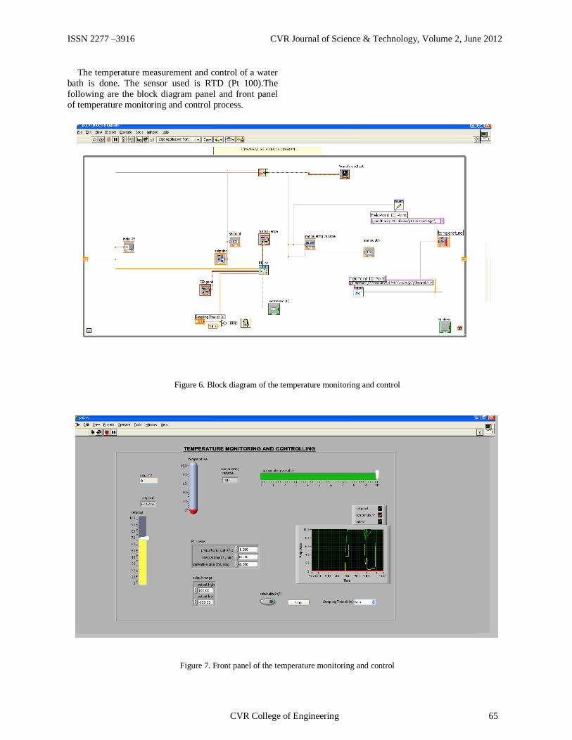
ISSN 2277 –3916 CVR Journal of Science & Technology, Volume 2, June 2012
The temperature measurement and control of a water
bath is done. The sensor used is RTD (Pt 100).The
following are the block diagram panel and front panel
of temperature monitoring and control process.
V. RESULTS
Figure 6. Block diagram of the temperature monitoring and control
Figure 7. Front panel of the temperature monitoring and control
CVR College of Engineering 65

ISSN 2277 –3916 CVR Journal of Science & Technology, Volume 2, June 2012
The results are shown below. The level and
temperature of kerosene tank and water bath
respectively were monitored and controlled through
internet. Strain of cantilever beam was monitored
through internet.
Figure 8.Graph of the level monitoring and control using PID
control
Figure 9.Graph of the temperature monitoring and control using PID control
Figure 10. Internet Access
CONCLUSION AND FUTURE ENHANCEMENT
This paper deals with the process variable acquisition
and control of level, temperature and also monitoring of
process variable like level, temperature and strain
through internet using Lab View. This is something
which is different from the traditional practice. The
general procedure is to dump the PID control algorithm
into a microcontroller, now anyone adept at
microcontroller programming will not agree with us
that, the program runs into pages and more. So if the
process is a real time control loop. The same task has been achieved by us within a single page.
The controller’s output which we have obtained is to
be signal conditioned to match the voltage level’s of the
final control element, SCR (silicon controlled rectifier
in our case), therefore there still exists some complexity
and thought process to be put into. So as a small scale
demonstration we have shown the control using an LED
at the output. The intensity of the LED output light
varied as the PID control also varied.
The process of tuning the controller used by us is not
completely scientific and therefore we would
recommend an improvement in that part. There exists a myriad of ways which can be implemented viz. Z-N
method, PRC method etc.
We would like to conclude by leaving it to the
readers to ponder over the utility of the above project
reminding them that the process can be a part of a
larger project which might include more number of
parameters to be controlled and the system being more
complex.
ACKNOWLEDGEMENT
We thank the authorities of C.V.R. College of
Engineering for providing support for this research work.
REFERENCES
[1] Barry E. Paton 1999,” LabVIEW Graphical Programming for Instrumentation”. Prentice Hall
PTP, New Jersey, U.S.A. [2] Curtis D. Johnson 1984,” Microprocessor-Based
Process Control”. Prentice-Hall International, Inc Englewood Cliffs, NJ, U.S.A.
[3] DE-LORENZO, 2002, Electronic Laboratory,” (Basic Board To Study Temperature Regulation)”.DL.2155RGT1, Dl.2155RGT2, Milano, Italy.
[4] Donald R. Coughanowr, 1991,”Process Systems Analysis and Control”. McGraw-Hill, Inc., Singapore.
[5] Gary W. Johnson, 1994. “LabVIEW Graphical Programming”. McGraw-Hill, Inc., New York, U.S.A.
[6] J. Michael Jacob, 1989,” Industrial Control Electronics”. Prentice-Hall International, Inc., New Jersey, U.S.A.
[7] National Instruments, 2002, LabVIEW Basics Introduction, Course Manual, U.S.A.
[8] National Instruments, 1996, “LabVIEW Graphical Programming for Instrumentation”. User Manual. New Jersey, U.S.A.
66 CVR College of Engineering

ISSN 2277 –3916 CVR Journal of Science & Technology, Volume 2, June 2012
Numerical Solution Of Oscillatory Motion Of
Dusty Memory Fluid Through Porous Media D.Sreenivas
1 and B.Shankar
2
1CVR College of Engineering, Department of H&S, Ibrahimpatan, R.R.District, A.P., India
Email:[email protected] 2Osmania University, Department of Mathematics, Hyderabad, A.P., India
Email: [email protected]
Abstract—The solution of oscillatory motion of dusty
memory fluid through porous media by finite element
method is obtained; expressions for the velocity of fluid,
dust and skin friction are also obtained. The effects of
various parameters on above are shown graphically and
discussed.
Index Terms—Oscillatory motion, Dusty memory fluid,
Porous medium.
I. INTRODUCTION
The study of flow dusty fluids has important
applications in the fields of fluidization, combustion use
of dust in gas cooling systems, centrifugal separation of
matter from fluid, petroleum industry, purification of
crude oil, polymer technology and fluid droplets sprays.
The constitutive equation for the rheological equations
of state for a memory fluid (Walter‟s liquid B model)
given by Walter (1960, 1962).Grover (1968) studied the
motion of an incompressible viscous fluid bounded by
two infinite plates, the upper one is fixed and the other
executing a simple harmonic oscillation in its own plane. Siddappa and Shanker Hegde (1972) have extended the
Grover‟s work for oscillatory motion of memory fluid
given by Rivlin-Ericksen constitutive equation. Sattar and
Ahmed (2007) obtained the numerical solution of Non-
Newtonian fluid. Rafiuddin et al. (2006) derived the
exact solution of oscillatory motion of a memory fluid
through porous media with a horizontal force. Ramu et al.
(2010) presented the numerical solution of the above
problem.
The aim of the present investigation is to study
oscillatory motion of dusty memory fluid through porous medium which is bounded by two infinite parallel plates
and both the plates are vibrating with same amplitude and
frequency.
II. FORMULATION OF THE PROBLEM
Consider the oscillatory motion of a dusty memory
fluid bounded by two infinite parallel plates through a
porous medium. Let the direction of motion of the fluid
be along the x-axis, which is chosen along the lower plate
and the y-axis be perpendicular to it. Let (u, v, w) be the
velocity components of the fluid. For the present study, v
= w = 0. The velocity of the oscillating plate at any
instant is taken as u = Re (u0
e- iωt
), where „Re‟ represents
the real part. For convenience we drop the expression
„Re‟, but we take the real part of the final result. The
equation of motion governing the dusty memory flow is
of the form
(2.1)
(2.2)
and the equation of continuity is
∂u/∂x= 0 (2.3)
The equation will now be made dimensionless by
introducing the non-dimensional quantities.
(2.4)
Substituting in (2.1) & (2.2) dropping the dashes for
simplicity, we get
(2.5)
(2.6)
Eliminating vp from (2.5) making use of (2.6), we get
(2.7) Where
K– stock‟s coefficient of resistance (6πaμ) for
spherical dust particles,
a – average radius of dust particle,
µ – viscosity of the fluid,
l– mNo/ ρ mass concentration of dust particle,
CVR College of Engineering 67

ISSN 2277 –3916 CVR Journal of Science & Technology, Volume 2, June 2012
ρ – density of fluid,
m –average mass of dust particle,
No– number of dust particle per unit volume,
β–kinematic visco-elasticity
τ – m/K relaxation time,
α – kinematic viscosity,
γ –permeability parameter,
yo –characteristic velocity,
s – memory parameter.
III. SOLUTION OF THE PROBLEM
Let the lower plate execute simple harmonic
oscillations in its own plane whereas the upper plate is
fixed .In this case the boundary conditions are
y = 0 , u = uo e –i ω t
,
y = 2yo , u = uo e –i ω t
(3.1)
Where 2y0 is the clearance distance between the
vibrating plate and fixed plate.
Introducing dimensionless frequency ω given by ω =
ω yo
2/α and using (2.4), the boundary conditions in (3.1)
in dimensionless form reduces to
y = 0, u = e –i ω t
,
y = 2, u = e –i ω t
(3.2) To solve the equation (2.5), we assume the solution of
the form
u = g (y) e –i ω t (3.3)
Now applying the boundary conditions (3.2) to (3.3),
we get
y = 0, g(y) = 1,
y = 2, g(y) = 1 (3.4) Substituting (3.3) into (2.5), we have
g ' '( y ) + mg ( y ) = 0 (3.5) Where
(3.6)
The equation (3.5) is an ordinary differential equation
with boundary conditions (3.2) through finite element method using Galerkin method, the solution of (3.5) is
given by
g(y)=1+ay(y-2) (3.7)
The velocity distribution is given by (3.3)
The real part of the velocity of the fluid is given by
u(y)=[1+1
G y(y-2)] cos t+[1
H y(y-2)]sin t
(3.8)
Skin friction at the lower plate is given by
0)(
yy
uC -2(
1G cos t +
1H sin t)
(3.9) Dust velocity is given by
))2(1)(1
(22)2((cos
))2()1
(22)2((sin
1111
1111
yyGl
sHGyyHt
yyHl
GsHyyGt
lV
p
(3.10)
))1
(22(cos)2)1
(2(sin)(1111
Gl
HtHl
Gtly
VD
p
(3.11)
Where the constants are not given for the sake of
brevity
DISCUSSION AND CONCLUSION
From fig-1 it is found that as permeability parameter
(γ) and memory parameter (s) increase, fluid velocity (u)
increases and from fig-2 we see that mass concentration
(l) increases dust velocity (Vp) decreases and Vp
increases with relaxation time (τ) , from the middle of the
plates the trend is opposite for both. From fig-3 it is observed that skin friction (C) decreases with
permeability parameter and memory parameter. Skin
friction in fig-4 for the dust case (D) decreases with mass
concentration and increases with relaxation time.
We can further extend this work by studying
oscillatory motion of dusty memory fluid through porous
medium which is bounded by two infinite parallel plates
by applying horizontal force following Lamb.
REFERENCES
[1] Walter, K. Quart. Jour. Mech. Applied Math. 13, pp. 444, 1960.
[2] Walter, K. Quat. Jour. Mech Applied Math. 15 pp. 136, 1962.
[3] Grover, G.K Proc. Int. Soc. Theoretical and Applied Mechanics pp.89, 1968.
0
0.1
0.2
0.3
0.4
0.5
0.6
0.7
0.8
0.9
0 0.5 1 1.5 2 2.5
0
0.2
0.4
0.6
0.8
1
1.2
1.4
1.6
1.8
0 0.5 1 1.5
0
5
10
15
20
25
0 0.5 1 1.5
-10
-8
-6
-4
-2
0
2
4
0 0.5 1 1.5 2 2.5
Fig 1.velocity profile for fixed values of
2,2.0,6.0,1 lt Fig 2.dust velocity profile for fixed values of o f
2,5.0,6.0,1 st
Fig 3.skin friction for fixed values of
2,2.0,6.0,1 lt Fig 4.skin friction of dust profile for fixed values of
2,5.0,6.0,1 st
7.2.
5.4.
5.2.
III
II
I
s
7.2.
5.4.
5.2.
III
II
I
s
4.2
2.4
2.2
III
II
I
l
4.2
2.4
2.2
III
II
I
l
u
y I
II
III
pv
y
C t
t
D
III
I II
II
III I
III
I
II
68 CVR College of Engineering

ISSN 2277 –3916 CVR Journal of Science & Technology, Volume 2, June 2012
[4] Siddappa, B. and Shanker Hegde Progress of Mathematics B.H.U., 6 (2):pp15, 1972.
[5] Rajput (1991) M.Phil. Thesis, Gulberga University, Gulberga.
[6] Arjumand, S. and Ahmed Waheedullah Journal of pure and applied physics vol. 19 No.2 (April- June) pp. 69-75, 2007.
[7] Addepalli Ramu, M.V. Ramana Murthy, Rafiuddin, Arjumand Sattar and Adeeb Nazia Atti Della Fondazione Giorgio Ronchi sept-oct; LXV 5, pp.
607-618, 2010. [8] Lamb, S.Horance 1932:Hydrodynamics.Sixth edition
Cambridge University Press. [9] Syed Amanullah Hussaini , M V Ramana Murthy,
Ahmed Waheedullah, Rafiuddin-Numerical solution of oscillatatory motion of a dusty viscous fluid-Atti Della “Fondazoine Giorgio Ronchi”-Anno LXVI,2011-N.6.
CVR College of Engineering 69

ISSN 2277 –3916 CVR Journal of Science & Technology, Volume 2, June 2012
Next Generation Network – A Study On QOS
Mechanisms Dr. B. B. Jayasingh1 and Sumitra Mallick2
1CVR College of Engineering, Department of IT, Ibrahimpatan, R.R.District, A.P., India
Email: [email protected] 2Guru Nanak Institute of Technology, Department of IT, Ibrahimpatan, R.R.District, A.P., India
Email: [email protected]
Abstract-Next Generation Network (NGN) being an IP
based network enables customers to receive voice, data
and video over the same network. NGN offers reduced
network and operational complexity resulting in better
and reliable service. It offers unrestricted access by users
to different service providers also supporting generalized
mobility. Next Generation Network is capable of
converging heterogeneous networks and provides
converged services. Resource and Admission Control
Function(RACF) is needed to support QoS of the SIP
based converged services, which are per session based real
time services, such as IP telephony and video telephony.
We study the architecture of NGN though the transition
from the legacy PSTN to an IP based NGN is an
important issue and the QoS control scheme has a strong
tendency of focusing on the edge and the access networks.
We also present a hierarchical QoS control architecture
for improvement of simplicity and scalability in the whole
view of the NGN using a divide and conquer strategy
which separates interesting objects that are the core and
the access networks. We present the Markova modeling of
the per session based centralized control scheme and the
distributed traffic engineering scheme(e.g. RSVPTE, CR-
LDP) for the verification of control costs.
Index Terms—NGN, RACF, SCF, CCM, System Sojourn
Time.
I. INTRODUCTION
Nowadays the IP telecommunication market is characterized by an increasing demand for multimedia
and real-time communication services, such as Video
on Demand, IPTV and Grid Computing, with strict
connectivity requirements about bandwidth, packet
delay and jitter [1]. Unfortunately, current Internet
architecture does not fully support the provisioning of
end-to-end emerging broadband services since the
Internet service model does not envisage a generalized
end-to-end Quality of Service (QoS) support.
Next Generation Network (NGN) is a packet
oriented network architecture, standardized by the
International Telecommunication Union –Telecommunication Standardization Sector (ITU-T)
that supports end-to-end service provisioning based on
different QOS-enabled transport technologies. The
NGN services include multimedia services (e.g., IPTV),
content delivery services (e.g., audio and video
streaming), and existing fixed and mobile telephone.
NGN being an IP based network enables customers
to receive voice, data and video over the same network.
NGN offers reduced network and operational
complexity resulting in better and reliable service. It
offers unrestricted access by users to different service
providers also supporting generalized mobility. In the
course of transition from the legacy PSTN to an IP based NGN there are many issues [2] which need to be
addressed. We would be addressing the issues relating
to regulation and interconnection which arise in the
course of migration to NGN.
Next Generation Network (NGN) has been on the
implementation phase, primarily focused on a
replacement of PSTN. In Japan, the largest national
telecom carrier NTT group has announced to start NGN
services in March 2008. NTT has also released a set of
documents on the preliminary interface condition and
service specification for connecting to their NGN
networks. The primary target for NGN is to replace the existing
PSTN and ISDN, by introducing highly-reliable
networks based on Internet Protocol (IP) and the related
technologies. For example, telephone signaling network
will be replaced by Session Initiation Protocol (SIP),
and the voice transmission will use connectionless
protocols such as Realtime Transfer Protocol (RTP) [3].
The current Internet is a set of multiple networks
which are arbitrarily connected together in various
Internet exchanges (IXes), under multitude of bilateral
and multilateral agreements between individual Internet Service Providers (ISPs). Some ISPs own the physical
links while some use the links provided by the others.
Forwarding data between different ISPs are controlled
by the policy-based routing protocol, such as Border
Gateway Protocol (BGP) [4]. While the current Internet
allows open and diverse connectivities as an inter-
network of multiple ISPs, the routing has become too
complex and a high-cost task for each router. Routing
between ISPs are only controlled by the forwarding
path between the Autonomous Systems (ASes), a set of
70 CVR College of Engineering

ISSN 2277 –3916 CVR Journal of Science & Technology, Volume 2, June 2012
multiple IP networks representing an ISP, since BGP is
a path vector routing protocol based on policies and
rule-sets.
As the number of networks connected to the current
Internet increases rapidly, the minimal service
conditions between two arbitrary networks get worse with higher latency of packets, instability of multi-ISP
routes, and the financial and social conditions of transit
ISPs and IXes [5]. Another NGN’s perspective is to
provide a reliable set of services which have already
been commercialized on the current Internet, under the
control of single management entity, such as a telecom
carrier company, which is a completely different management model from the current Internet. NGN
networks will introduce prioritized packet forwarding
based of Differentiated Services (DiffServ) by using the priority field in each IP packet and with strict priority
queueing strategy, so that it can provide real-time
services such as telephony and video multicast with no
interruption by other services with less real-time
demands, such as email and Web.
NGN has layered architecture which consists of a service stratum as a session control layer and a
transport stratum as a packet transmission layer [6].
MPLS (Multi Packet Label Switched) is adopted as a
packet core network technology of transport stratum [7]
and the QoS control on MPLS-TE which is considered
to be the standardization. NGN needs QoS control in
the view of traffic engineering for the purpose of
providing SIP based multimedia services such as IP
telephony, video IP telephony, and video conference
etc. Herein, NGN architecture defines Resource and
Admission Control Function (RACF) in the transport stratum [7].
II. NGN ARCHITECTURE
This section provides an outline of the NGN Release
architecture and the current state-of-the-art of the
standardized features. An extensive outline of the ITU-
T NGN is already provided in [8], while this section is
strictly focused on the NGN mechanisms for the
provisioning of QOS-guaranteed connectivity services.
Figure. 1. The NGN architecture
Referring to Fig. 1, the NGN architecture is
composed of two sets of functionalities, named Service
Stratum and Transport Stratum. To the purpose of this
work, the main Service Stratum functional entity is the
Service Control Function (SCF). SCF functionalities
are specific of a given class of services. SCF performs end-users Authentication, Authorization, and
Accounting (AAA) and processes service requests
issued by authorized end-users. In particular, by
interacting with the Transport Stratum, SCF checks the
availability of the network resources and authorizes the
network resources reservation needed for the
provisioning of the requested service. An example of
SCF is the Core IP Multimedia Subsystem (IMS) that
inherits and possibly extends a subset of the IMS
functionalities standardized by 3rd Generation
Partnership Project (3GPP) for the provisioning of
Session Initiation Protocol (SIP)-based multimedia services [9].
The Transport Stratum provides IP connectivity
services for the benefit of SCFs under the authority of
the Network Attachment Control Function (NACF) and
the Resource and Admission Control Function (RACF).
The NACF is a functional entity that, on receiving a
service request issued by an end-user, authenticates the
user identity and authorizes the use of network
resources based on user profiles. In addition, NACF
may supply RACF with the network configuration
parameters needed to support the service provisioning. The RACF is the functional entity that enables the
SCFs to control network functionalities such as the
bandwidth reservation and allocation, the packet
filtering, the Network Address and Port Translation
(NAPT) while hiding the network technology and
topology details. A RACF instance is able to control the
network resources belonging to the same administrative
domain as shown in Fig.1.
The RACF consists of two specialized functional
entities, namely the Policy Decision Functional Entity
(PD-FE) and Transport Resource Control Functional
Entity (TRC-FE). The PD-FE is the single contact point between any SCF and the Transport Stratum. It makes
the final decision about admission, reservation, and
control of the network resources supporting the
provisioning of the SCF services. The PD-FE decisions
are based on (i) the preloaded policy rules decided by
the network operator, (ii) the service information
provided by the SCF via Rs interface, (iii) the result of
resource authorization provided by the NACF via Ru
interface, (iv) the outcome of resource admission
provided by the TRC-FEs via Rt interface. In addition,
the PD-FE may enforce decisions by interacting with a set of Policy Enforcement Functional Entities (PE-FEs)
via Rw interface. The PE-FEs are the functional blocks
that control the technology-independent network
service functionalities implemented at the boundaries of
the network such as the NAPT. A set of PD-FEs may
CVR College of Engineering 71

ISSN 2277 –3916 CVR Journal of Science & Technology, Volume 2, June 2012
interoperate for the seamless provisioning of
connectivity services across a multidomain network.
PD-FEs within the same administrative domain
communicate via Rd interface while PD-FEs belonging
to different administrative domains communicate via Ri
interface. The TRC-FE performs technology-dependent
admission decisions over the network resources on
behalf of PD-FE. Those decisions are based on the
requirements received from the PD-FE and on the
information previously collected by the TRC-FE about
the network topology and the status of the network
resources. TRC-FE may interact with a set of Transport
Resource Enforcement Functional Entities (TREFEs)
via the Rn interface to enforce its decisions over the
network. A network domain may contain multiple
instances of TRC-FEs controlling different areas. The
TRC-FEs belonging to the same administrative domain directly communicate via the Rp interface. TRC-FEs
belonging to different administrative domains indirectly
communicate through the corresponding PD-FEs via
the Ri interface.
The NGN Transport Stratum comprises both access
and core networks. In NGN an access network is meant
as a network that “takes care of end-users' access to the
network as well as collecting and aggregating the traffic
coming from these accesses towards the core network”
[10]. An NGN terminal interacts with the NGN access
network through the corresponding Customer Premise Equipment (CPE) to exchange signalling messages with
an instance of SCF. Also, the NGN terminal sends data
traffic through the CPE to the Transport Functions,
defined in [10] as the set of Transport Stratum entities
that interact with the RACF.
III. QOS CONTROL ARCHITECTURE
Although NGN architecture which provides a carrier
grade constraint route scheme is different from Internet
architecture to support a liberal route scheme, the
researches of QOS control in Internet are still of use.
The research of Broad Band (BB) architectures gives a
suggestion of hybrid architecture as well as an explanation of a centralized and a distributed
Architecture. The hybrid architecture suggested in [11]
approaches to improve the resource utilization of the
admission mechanism while balancing it with the BBs’
processing loads through the adaptation of the
centralized and the distributed architectures. However
the hybrid architecture pays attention to information
synchronization and work load distribution. This
architecture provides a coordinate function between two
areas. As the coordinate function does not take part in
database accesses, there is no issue of consistency. This architecture is expected to handle real time resource and
admission control operations for supporting SIP based
converged services such as IP telephony and video IP
telephony services in NGN. We anticipate that this
architecture solves a scalability issue through process
load balancing and has advantages of the centralized
control scheme which provides high resource
utilization, strong consistency, and simplicity. Figure 2
shows the suggested hierarchical architecture in this paper. The Control Coordination Layer (CCL) is
deployed in the upper layer and the Resource and
Admission Control Layer (RACL) is in the lower. The
Control Coordination Manager (CCM) is located in the
CCL. RACL approaches a divide and conquer strategy
so that the complexity of traffic engineering is
decreased. Access Resource and Admission Control
Manager (ARACM) takes charge of the access network
and Core Resource and Admission Manager (CRACM)
takes charge of the core network.
Figure 2. Hierarchical resource and admission control architecture
The operation mechanism of this architecture is as
follow:
1. Whenever a calling CPE initiates SIP signaling
to a called CPE, the Session Control Function
(SCF) transfers information(e.g. bandwidth
constraint) for acquiring an appropriate route to the CCM.
2. CCM request to CRACM and ARACM which
handles the access networks of the calling and
the called CPE belonging to.
3. CRACM searches a matched ER-LSP route in
the core network and ARACM finds an
appropriate route in the access network
concurrently.
4. CRACM and ARACM return admission
results to CCM.
72 CVR College of Engineering

ISSN 2277 –3916 CVR Journal of Science & Technology, Volume 2, June 2012
5. CCM decides final admission result based on
the results of CRACM and ARACM.
6. If the final admission result is positive, CCM
responds to SCF a call admission and requests
to CRACM and ARACM resource
reservations concurrently. And then CRACM and ARACM reserve resources.
7. If the result is negative, CCM responds to SCF
a call rejection.
A. QOS Mechanisms
The ways to assure end-to-end QoS is through
priority scheduling, resource reservation and admission control mechanisms.
Priority scheduling:NGN is based on IPv6 and RACS
calculate the number of hops and remarks hop limit.
If the number of hop limit is large it provides
higher priority.
If the number of hop limit is small it provides
lower priority.
Let’s assume average minimum bound of
packet delay is r ms
Average propagation delay of one hop is p ms
There are two QOS class: high and low
Average queuing delay of high priority per one
hop is h ms
Average queuing delay of low priority per one
hop is l ms
Let there are two end to end connections:
longest and shortest routes
Longest takes d hops to reach destination
Shortest takes s hops to reach destination
Longest route-worst case:
(p+h)*d ms must be smaller than r ms
shortest route-worst case: (p+h)*s ms and it is much lower than r ms if (p+l)*s
ms is much smaller than r ms, it can use low priority for
the shorted route means there are the route which is
(p+h)*(l-d)/s - p hops to get low priority QOS request
to high priority.
B. Centralized QOS Control Scheme
In this section, we introduce a Centralized MPLSTE
(CMPLS-TE (Traffic Engineering)) which uses a
centralized scheme for the majority of NGN carriers
who use DiffServ aware MPLS in the core. MPLS-TE
is mainly dealt in the management plane so far,
however the suggested scheme approaches from the
control plane of the transport stratum as fig 1 shows.
CMPLS-TE has advantages compared with the
distributed MPLS-TE(e.g. RSVP-TE). It improves
reliability because control messages such as LSP (Label
Switch Path) setup and release are transferred through a control channel separated from a data channel. It
improves efficiency as the scheme supports the setup,
release, and modification of a bidirectional LSP and a
multicast LSP just a one-shot control. It is expected to
be a fast reroute because it is possible to control a
reroute in an affected problem area only instead of a
crank-back of whole paths along the LSP. It has
flexibility of LSP route selection algorithm so that it
adopts several algorithms simultaneously and is easier to update a new algorithm. On the other hand, it needs
consideration with regards to a router failure or a failure
of whole link which consists of a control channel. A
manual management approach is needed in these cases.
We also expect that the scheme overcomes a scalability
issue in the one NGN carrier domain scale because of
nowadays’ blade server capacities and management of
LSP paths limitations (e.g. LSP merge, LSP
modification).
System sojourn time (E(T)) - the total waiting time
from an arrival to a departure from a system - is a
representative performance metric [12]. Therefore we define E(T) for LSP setup as a control cost and present
models of RSVP-TE and CMPLS-TE for acquiring the
control costs. In the RSVP-TE scheme, RSVP-TE
transfers a PATH message from ingress LER (Label
Edge Router) to egress LER through intermediate LSRs
(Label Switch Router) along the route. Then it allocates
bandwidths of the LERs and LSRs of the LSP through
transferring a RESV message backward for a
completion of ER-LSP setup as shown in figure 3. We
presume a bidirectional symmetric LSP setup and
assume that processing time for the messages is much bigger than transmission and propagation delay for the
messages. EDist(T) of RSVP-TE represents equation
which means sum of processing time of the PATH and
the RESV message for the downstream uni-direction
and for the upstream uni-direction LSP.
Figure 3. RSVP-TE ER-LSP setup scheme
The central manager sends an LSP_Setup_Request message to ingress LER via intermediate LSRs to
egress LER and reports to the CCM the result of
bandwidth reservation after each LER and LSR
CVR College of Engineering 73
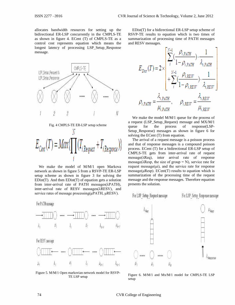
ISSN 2277 –3916 CVR Journal of Science & Technology, Volume 2, June 2012
allocates bandwidth resources for setting up the
bidirectional ER-LSP concurrently in the CMPLS-TE
as shown in figure 4. ECent (T) of CMPLS-TE as a
control cost represents equation which means the
longest latency of processing LSP_Setup_Response
message.
Fig. 4 CMPLS-TE ER-LSP setup scheme
We make the model of M/M/1 open Markova
network as shown in figure 5 from a RSVP-TE ER-LSP
setup scheme as shown in figure 3 for solving the
EDist(T). And then EDist(T) of equation gets a solution
from inter-arrival rate of PATH messages(λPATH),
inter-arrival rate of RESV messages(λRESV), and
service rates of message processing(μPATH, μRESV).
Figure 5. M/M/1 Open markovian network model for RSVP-TE LSP setup
EDist(T) for a bidirectional ER-LSP setup scheme of
RSVP-TE results to equation which is two times of
summarization of processing time of PATH messages
and RESV messages.
We make the model M/M/1 queue for the process of a request (LSP_Setup_Request) message and MX/M/1
queue for the process of response(LSP-
Setup_Response) messages as shown in figure 6 for
solving the ECent (T) from equation.
The arrival of a request message is a poisson process
and that of response messages is a compound poisson
process. ECent (T) for a bidirectional ER-LSP setup of
CMPLS-TE gets from inter-arrival rate of request
message(λReq), inter arrival rate of response
message(λResp, the size of group = N), service rate for
request message(μi), and the service rate for response
message(μResp). ECent(T) results to equation which is summarization of the processing time of the request
message and the response messages. Therefore equation
presents the solution.
Figure 6. M/M/1 and Mx/M/1 model for CMPLS-TE LSP setup
74 CVR College of Engineering

ISSN 2277 –3916 CVR Journal of Science & Technology, Volume 2, June 2012
We assume the followings for comparing of the
ECent(T) and the EDist(T) according to the N size(the
number of the LERs along the arbitrary ER-LSP).
1. Assuming an arbitrary absolute value of μ, and
setting up μPATH = μRESV = 2μ, μi = μ, μResp = α·μ (α is a
constant coefficient). 2. Assuming an arbitrary absolute value of λ, and
setting up λ= 1, λPATH = λRESV = λReq = λResp = λ.
Figure 6 shows that the value of the ECent(T) and
the EDist(T) according to the size of N, when the value
of μ is varied. Dotted lines show when the value of μ is
30, and solid lines show when μ is 50. In the condition
of general assumptions, the ECent(T) is lower than the
EDist(T) therefore we conclude that ECent(T) is
superior for the control cost in general.
Figure 7. Comparison of control cost on condition of mu=30 and 50
CONCLUSION
We reviewed the novel NGN architecture with RACF
entity, able to control dynamically and to coordinate the
QOS-guaranteed connectivity. NGN has brought a
revolution in mobile networks and some questions are
yet to be addressed in implementing it but the situation
is changing fast and NGN is capturing the mobile
market. The demand for various services to be provided
on a single platform has increased. We understand the
primary motivation of NGN is the replacement of the
legacy telecom carrier networks, with the inexpensive
equipments available for the Internet protocols. Many
Internet users expect NGN to be better than the current Internet and ensuring access to the existing Internet
services. The advantage of NGN is having admission
control mechanism that reduces network resource
reservation complex in unit of log scale. The reserved
resources in a route has less delay in centralized
approach compared to distributed approach that shows
the NGN QOS.
REFERENCES
[1] [1] F. Baroncelli, B. Martini, V. Martini and P.
Castoldi, “Supporting Control Plane-enabled Transport Networks within ITU-T Next Generation Network (NGN) architecture”, 978-1-4244-2066-7/08/$25.00 ©2008 IEEE, pp. 271-278.
[2] Dr. Mustafa Shakir, “Challenging Issues in NGN Implementation and Regulation”, 978-1-4244-3709-2/10©2010 IEEE
[3] H. Schulzrinne and S. Casner and R. Frederick and V. Jacobson, “RTP: A Transport Protocol for Real-Time Applications,” July 2003, RFC3550.
[4] Y. Rekhter, T. Li, and S. Hares, “A Border Gateway Protocol 4 (BGP-4),” January 2006, RFC4271.
[5] Kenji Rikitake and Koji Nakao, “NGN and internet: from coexistence to integration”, First ITU-T Kaleidoscope Academic Conference, 92-61-12441-
0/CFP0838E © 2008 ITU, japan. [6] Keith Knightson, Naotaka Morita, and Thomas
Towle, “NGN Architecture: Generic Principles, Functional Architecture, and Implementation”, IEEE Communications Magazine, vol. 43, no. 10, pp 49-56, Oct. 2005.
[7] Keith Knightson, Naotaka Morita, and Thomas Towle, “NGN Architecture: Generic Principles, Functional Architecture, and Implementation”,
IEEE Communications Magazine, vol. 43, no. 10, pp 49-56, Oct. 2005.
[8] Keith Knightson et al “NGN Architecture: Generic Principles Functional Architecture, and Implementation” Communications Magazine, IEEE, Oct. 2005, Volume 43, Issue 10.
[9] ITU-T Y.2021, “IMS for Next Generation Networks”, September 2006.
[10] ITU-T Y.2012, “Functional requirements and architecture of the NGN release 1”, September 2006.
[11] Ch. Bouras and K. Stamos, “Examining the Benefits of a Hybrid Distributed Architecture for Bandwidth Brokers”, in Proc. IPCCC’05, 2005, Paper 10.1109/PCCC, pp. 491-498.
[12] Kwon Cho, Koji OKAMURA, “A Centralized
Resource and Admission Control Scheme for NGN Core Networks”, Graduate School of Information Science and Electrical Engineering, Kyushu University 6-10-1 Hakozaki, Higashi-ku, Fukuoka, 812-8581, Japan.
CVR College of Engineering 75

ISSN 2277 –3916 CVR Journal of Science & Technology, Volume 2, June 2012
Extended AODV For Multi-Hop WMN S.Jyothsna
CVR College of Engineering, Department of IT, Ibrahimpatan, R.R.District, A.P., India
Email: [email protected]
Abstract-Wireless Mesh Networks (WMN) consists
of mesh routers and mesh clients, where mesh
routers have minimal mobility and form the
backbone of WMNs. They provide network access
for both mesh and conventional clients. Existing
Adhoc On Demand Distance Vector(AODV)
Protocol was designed to simply yield the shortest
path between a given source and its destination.
This routing Protocol is not suitable for Wireless
Mesh Backbone since it do not consider the
impairments of wireless channels. we propose a
new routing metric called Expected Transmission
Count(ETX) and use this metric instead of the
minimum hop count metric to find routes that
result in higher throughputs. we will integrate
AODV with the ETX metric. We show that ETX
metric is superior to the hop count in terms of
finding paths with higher throughputs.
Index Terms-WMN, AODV, Routing Protocol,
Routing Metric, ETX.
I. INTRODUCTION
1.1 WMN
WMNs are comprised of two types of nodes
Mesh Router and Mesh Client. Along with the
routing capability for gateway/bridge functions
existing in a conventional wireless router, a mesh
router supports additional routing functions to
provide a platform for mesh networking. Mesh routers generally have minimal mobility and
their purpose is basically formation of mesh
backbone for the mesh clients. The
gateway/bridge functionalities in mesh routers
enable the integration of WMNs with various
other networks. Wireless Mesh routers enable
conventional nodes equipped with wireless
network interface cards (NICs) to connect
directly to WMNs. Ethernet can be used to
access WMNs by connecting to wireless mesh
routers when wireless NICs are not available.
1.2 Routing Metrics
Metrics are foundations to find the high
performance routing path between the source and
destination. A node measures some basic
elements for the link to its neighbors including
packet loss, delay, hop count etc. based on these
fundamental elements wireless node reassembles
them into a new parameter, the radio metric, to
describe the state of the link. Some popular radio
metrics have been proposed recently. Per-hop
RTT, Pkt Pair, ETX and ETT. ETX, proposed by
De Counto, estimates the number of
retransmissions needed to send unicast packets
by measuring the loss rate of broadcast packets between pairs of neighboring nodes.
II. RELATED WORK
Protocols such as DSR and AODV were
designed to simply yield the shortest path
between a given source and its destination. They do not consider the effects and impairments of
wireless channels.
2.1 Our Contribution
By considering the effect of packet losses on
wireless links, we define a new metric called
Expected Transmission Count (ETX) and use this metric instead of the minimum hop count
metric to find routes that result in higher
throughputs. Links with higher loss rates require
more retransmissions to successfully transmit a
packet and hence would have higher values of
ETX.
In multi-hop wireless networks,
communication quality depends on the route
from a source to a destination. In this paper, we
consider a one-dimensional multi-hop wireless
network where nodes are distributed randomly and theoretically analyze the relation between
communication quality and routing policy using
ETX, which is the predicted number of data
transmissions required to send a packet over that
link, including retransmissions. First, we
theoretically analyze the mean length of links,
the mean number of hops, and the mean route
ETX, which is the sum of the ETXs of all links
in a route. We compare hop count metric and
ETX in AODV, using the results of analysis and
show differences between these algorithms in the
route. We provide a comparative analysis of various
routing strategies that effect end to end
performance in WMN. We first improve well-
76 CVR College of Engineering
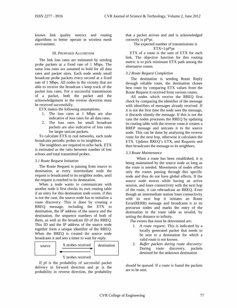
ISSN 2277 –3916 CVR Journal of Science & Technology, Volume 2, June 2012
known link quality metrics and routing
algorithms to better operate in wireless mesh
environment.
III. PROPOSED ALGORITHM
The link loss rates are estimated by sending
probe packets at a fixed rate of 1 Mbps. The
same loss rates are assumed to hold for all data
rates and packet sizes. Each node sends small
broadcast probe packets every second at a fixed
rate of 1 Mbps. All nodes in the vicinity that are
able to receive the broadcast s keep track of the
packet loss rates. For a successful transmission
of a packet, both the packet and the
acknowledgement in the reverse direction must
be received successfully. ETX makes the following assumptions.
1. The loss rates at 1 Mbps are also
indicative of loss rates for all data rates.
2. The loss rates for small broadcast
packets are also indicative of loss rates
for larger unicast packets.
To calculate ETX in real networks, each node
broadcasts periodic probes to its neighbors.
The neighbors are required to echo back. ETX
is estimated as the ratio between number of lost
echoes and total transmitted probes.
3.1 Route Request Initiation
The Route Request is passing from source to
destination, at every intermediate node the
request is broadcasted to its neighbor nodes, until
the request is reached to its destination.
When a node wants to communicate with another node it first checks its own routing table
if an entry for this destination node exists. if this
is not the case, the source node has to initialize a
route discovery. This is done by creating a
RREQ message, including the ETX to
destination, the IP address of the source and the
destination, the sequence numbers of both of
them, as well as the broadcast ID of the RREQ.
This ID and the IP address of the source node
together form a unique identifier of the RREQ.
When the RREQ is created the source node
broadcasts it and sets a timer to wait for reply.
If pf is the probability of successful packet
delivery in forward direction and pr is the
probability in reverse direction, the probability
that a packet arrives and and is acknowledged
correctly is pf*pr.
The expected number of transmissions is
ETX=1/pf*pr ETX of a route is the sum of ETX for each
link. The objective function for this routing
metric is to pick minimum ETX path among the
alternative routes.
3.2 Route Request Completion
The destination is sending Route Reply
through reliable route, the destination choses
best route by comparing ETX values from the
Route Request it received from various routes.
All nodes which receive the RREQ first
check by comparing the identifier of the message
with identifiers of messages already received. If
it is not the first time the node sees the message,
it discards silently the message. If this is not the
case the nodes processes the RREQ by updating
its routing table with the reverse route.it creates a
RREP message and unicasts it to the source node. This can be done by analyzing the reverse
route for the next hop, otherwise it calculates the
ETX. Updates RREQ’s ETX, and Requests and
then broadcasts the message to its neighbors.
3.3 Route Maintenance
When a route has been established, it is being maintained by the source node as long as
the route is needed. Movements of nodes effect
only the routes passing through this specific
node and thus do not have global effects. If the
source node moves while having an active
session, and loses connectivity with the next hop
of the route, it can rebroadcast an RREQ. Even
though an intermediate station loses connectivity
with its next hop it initiates an Route
Error(RERR) message and broadcasts it to its
precursor nodes and marks the entry of the destination in the route table as invalid, by
setting the distance to infinity.
The events that must be determined are:
1. A route request: This is indicated by a
locally generated packet that needs to
be sent to a destination for which a
valid route is not known.
2. Buffer packets during route discovery:
During route discovery, packets destined for the unknown destination
should be queued. If a route is found the packets
are to be sent.
source destination X probes received
Y probes received
CVR College of Engineering 77

ISSN 2277 –3916 CVR Journal of Science & Technology, Volume 2, June 2012
3. Update the lifetime of an active route:
This is indicated by a packet being
received from, sent to or forwarded to a
known destination. 4. Generate a RERR if a valid route does
not exist: If there is no known route to a
destination, the node must send a
RERR.
5. Generate a RERR during restart: After
the AODV routing protocol restarts, it
must send a RERR message to other
nodes attempting to use it as a router.
IV. RESULTS AND ANALYSIS
For the experiments, we choose hop-count
metric to provide baseline for performance comparison along with ETX.
4.1 Experimental setup
Our experiments are performed using NS-2
simulations. In our experiments, we choose the
10-node scenario,20-node scenario,50-node
scenario and 100-node scenario,120-node scenario,150-node scenario,180-node scenario.
For simulations, we choose the distances
between the nodes and their transmissions ranges
in such a way that both paths are independent
with the exception of sharing source and
destination.
4.2 Simulations
NS-2 is our simulation platform and we
implemented ETX with AODV routing protocol.
AODV is chosen because of its suitability to the
stationary scenario of wireless mesh networks. We have added probing mechanism in AODV
protocols where each node broadcasts a probe
packet after every 10 sec for ETX and the
receivers send back a unicast echo packet.
Sending time is embedded in the probe packet.
When a node receives an echo packet from a
neighbor, it calculates the delay. If the delay is
greater than a fix threshold i.e 10000 ms in our
experiments, the echo packet is dropped
otherwise, the node counts the dropped or lost
packets to calculate ETX. ETX uses the last ten
probes for computation. When a node receives routing table broadcast from a neighbor, it adds
the ETX value of the link to the neighbor to the
table entries and compares them with its own
table.
Constant bit rate (CBR) UDP traffic is used
with 1000 byte packets for various data rates
form source 0 to destination 3. UDP traffic
allows us to study the performance of routing
metric in the simplest settings without any
influence of transport protocol artifact. To
implement loss in non-preferred path, a node on
the path is made to drop random packets among all it receives according to specific probability of
loss. Each result is averaged over 10 simulation
runs and error bars in figures show 95%
confidence interval.
We got expected results for ETX
performance under lower data rate, but with
higher data rates ETX performance was
comparatively low. The results are shown
interestingly, when one path become much
worse than the other, ETX has better throughput,
i.e., lower loss rate than hop-count. Hop-count always has a lower buffer overflow loss than
ETX, because it does not use probes. However,
hop-count does not distinguish between higher or
lower loss paths. As a consequence, when losses
in one path becomes higher, packets dropped due
to bad channels become more significant than
packets dropped due to buffer overflow and
overall performance of hop-count metric is
worse than ETX. No.of Nodes vs throughput
By analyzing the results, we can observe the
throughput is more where ETX as the metric.
Because, by calculating the ETX values on the
links, nodes can chose the lower ETX paths i.e
reliable links.
CONCLUSION
5. Summary
In this paper, a survey of routing metric
carried out, we proposed and implemented ETX
enhancement over well known AODV routing
protocol. The prerequisites that a multi-radio
multi-channel mechanism must have are also
studied. Steps and method to be used for new
metrics are discussed.
Based on our experiments, we observed our
proposed Routing Protocol is performing better
78 CVR College of Engineering
ISSN 2277 –3916 CVR Journal of Science & Technology, Volume 2, June 2012
than existing AODV, since ETX chooses paths
based link quality rather than number of hops.
ETX finds routes that result in higher
throughputs. We show that ETX metric is superior to the hop count metric in terms of
finding paths with higher throughputs.
ETX chooses links with higher delivery ratio.
Buffer overflow loss in ETX is in general more
than that of hop count, which has no probing
mechanism.
REFERENCES
[1] R.Draves, J.Padhye, and B.Zill, ―Comparison of routing metrics for static multi-hop wireless networks,‖ in SIGCOMM ’04: Proceedings of the 2004 conference on Applications, technologies, architectures, and protocols for computer
communications, 2004, pp.133-144. [2] D.S.J.D. Couto, D. Aguayo, J.Bicket, and R.
Morris, ―A high throughput path metric for multi-hop wireless routing,‖ Wirel. Netw., vol. 11, no. 4, pp. 419-434, 2005.
[3] I.F. Akyildiz and W. Xudong, ―A survey on wireless mesh networks,‖ IEEE communications Magazine, vol. 43, pp.
23—30, 2005. [4] W.S.,B. Ishibashi, R. Boulaba, and D.
Meddour, ―Performance study of wireless mesh networks routing metrics ,‖ in Proc. IEEE/ACS AICCSA 2008, March-April 2008,pp. 1100-1106.
[5] S.Misra et al., ―Guide to Wireless Mesh Networks‖ Springler-Verlag London Limited 2009
[6] C. Perkins, E.Belding-Royer, S.Das. Ad hoc On-Demand Distance Vector (AODV) Routing, RFC 3561.
[7] ―The Network Simulator-ns-2.‖ from http://www.isi.edu/nsnam/ns.
CVR College of Engineering 79

ISSN 2277 –3916 CVR Journal of Science & Technology, Volume 2, June 2012
A Study On HR Practices In CVRCE Dr.B.Archana
1 and Prof.M.S.Bhat
2
1CVR College of Engineering, Department of M.S., Ibrahimpatan, R.R.District, A.P., India
Email: [email protected] 2CVR College of Engineering, Department of M.S., Ibrahimpatan, R.R.District, A.P., India
Email: [email protected]
Abstract—The studies on Human Resource
Practices are positively linked with employee
performance and institutional performance in the
education sector. On this perspective, this study
examines the various HR practices based on the
survey of the selected teaching employees of
CVRCE. The results of the study indicate a high
degree of satisfaction by the employees towards the
various HR practices being followed by the
institution.
Index Terms—HR Practices, Selected Teaching
Employees, CVRCE.
I. INTRODUCTION
CVR College of Engineering (CVRCE),
approved by AICTE and affiliated to JNT
University, Hyderabad was established in 2001.
It was ranked in the TOP-8 among all colleges in
Osmania University (OU) area during
EAMCET-2008 counseling. It was also ranked
as the #1 college among more than 420 colleges
in Andhra Pradesh that started in the last decade.
It is promoted by NRI Technology Professionals,
who were residents in the US. It is the expectation of its academic
community that it is on the successful path to be
in the TOP-5 amongst all colleges in OU area in
the next couple of years. The vision statement of
CVRCE is to become a premier educational
institution in India, offering the best technical
training inputs to its students. It is the only
Engineering college in entire Andhra Pradesh to
have achieved the following three major
accomplishments within the first 6 years of
existence - getting NBA accreditation, having record campus placements and getting funding of
>Rs.18 lakhs from central government agency.
To add a feather to its cap, it has Professors who
have previously worked at OU and JNTU.
‘Human Resources’ is a terminology used to
describe the individuals who make up the
workforce of an institution. It is also the name
of the function within an institution charged with
the overall responsibility for implementing
strategies and policies relating to the
management of individuals, (i.e., the human
resources). This function’s title is often
abbreviated to the initials ‘HR’. In other words,
Human means the people, who are working in
the organisation, Resources means the various
facilities available in the organisation and
Management means getting things done by others.
II. REVIEW OF LITERATURE
A number of researchers have reported that
HR practices are positively linked with
organisational and employee performance
(Guest [1] 2002; Gould-Williams [2], 2003;
Harley [3] 2002; Park et al [4], 2003; Wright et
al [5], 2003 and Tessema [6] 2006).These
researchers focused their studies in the
developing countries like India, which are
considered to be ‘Knowledge Societies’,
equipped with a suitable workforce. Hence, the focus is growing on the importance of quality
education delivery, which is done through
efficient employees of an efficient organisation.
In this context what matters most is to what
extent the educational institution facilitates its
employees in providing a quality education. In
this backdrop, this study makes an attempt to
identify the various HR Practices provided by
the institution (i.e., CVRCE) 7 to its selected
employees who are into teaching.
III. OBJECTIVES
To understand the demographics of the
selected teaching employees
To identify the employees’ perception
on performance
To identify the various factors related to
compensation practices
To identify the various factors related to
performance evaluation practices
To identify the various factors
considered for promotion practices
To identify the various factors related to turnover practices
To rank the various welfare practices
offered
80 CVR College of Engineering

ISSN 2277 –3916 CVR Journal of Science & Technology, Volume 2, June 2012
To rank the various opportunities
provided for career advancement
To analyse the overall assessment of
HR practices
IV. LIMITATIONS
The study was restricted only to the
employees who were in teaching. Thus,
omitting the non-teaching employees,
who were also associated with the
institution from past many years.
The teaching employees who had not
completed two and above years of
service were purposefully excluded for
the study.
V. METHODOLOGY
The various employees who were into teaching from various departments and those
who have completed two and above years of
their service from the same institution have been
selected for the purpose of the study. However,
the study is not census based and is purely on the
basis of Judgmental sampling method. The
selected teaching employees were from various
strata like Professors, Associate Professors,
Senior Assistant Professors and Assistant
Professors of all the departments of the
institution.
VI. DATA COLLECTION
The Primary data was collected through
personally administered structured
questionnaires. The questionnaires were tested
through a pilot survey about the consistency and
other measures. A total of 70 questionnaires
were administered to all the selected teaching
employees. However, only 50 of them were
received back, thus making the response rate to
be 71% which was a sufficient sample size for
analysis. The breakup of the responses based
upon various departments to which the selected teaching employees belonged to was: ECE (14),
EEE (4), CSE (3), IT (9), EIE (5), H&S (6),
MBA (4) and MCA (5).
For the purpose of data collection, the
questionnaire was categorized into nine sections
titled as: Demographics, Employee perception on
performance, Compensation practices,
Performance evaluation practices, Promotion
practices, Turnover practices, Welfare practices,
Opportunities for career advancement and
Overall assessment of HR practices; in all
containing 35 Questions. Most of the responses were marked by the selected teaching employees
on a five point Likert’s Scale (with endpoints: 1-
Strongly disagree, 5-Strongly agree) and few of
the responses were obtained through open ended
questions. For the purpose of the analysis of the
data, the responses on the scale against the
grades ‘Agree’ and ‘Strongly agree’ were clubbed up and the responses obtained under the
grades ‘Disagree’ and ‘Strongly disagree’ were
separately clubbed up. However, the responses
obtained against the grade ‘Neutral’ are shown
without any such clubbing. The required
secondary data was collected from the website,
brochures, newsletters and service manual of
CVRCE, which was used for framing the
objectives and designing the questionnaire for
the purpose of the study.
VII. FINDINGS
Objective 1
To understand the demographics of the
selected teaching employees.
TABLE I:
DEMOGRAPHICS
Gender No. of employees
Male 25
Female 25
Designation No. of employees
Assistant Professor 34
Sr. Asst. Professor 1
Associate Professor 11
Professor 4
Tenure of employment No. of employees
2 years 4
2-4 years 14
4-6 years 21
More than 6 years 11
Age group No. of employees
20-30 years 14
31-40 years 28
41-50 years 4
Above 51 years 4
Qualification No. of employees
Bachelors 11
Masters 31
M.Phil / MS 7
Doctorate 1
Mother tongue No. of employees
Telugu 36
Hindi 2
Others 12
Source: Questionnaire to the employees
The objective of Table 1 is to show the
composition of the demographics of the
respondents considered for the study.
As depicted above, male and female
teaching employees were 25 each.
Majority of them were in the strata of
Assistant Professor; were falling in the
tenure period of 4-6 years; were in the age group of 31-40 years; were holding
Masters Degree as their qualification
CVR College of Engineering 81

ISSN 2277 –3916 CVR Journal of Science & Technology, Volume 2, June 2012
and most of theirs Mother tongue was
Telugu.
Objective 2
To identify the ‘employees’ perception on
performance.
The selected teaching employees were
requested to opine about various factors
related to the perceptions of their
Performances. For which, 37 of them
have opined to have better
performances than their colleagues with similar qualifications, 11 of them
viewed to be average and only 2 of
them had disagreed to it.
42 of them were satisfied with their
performances.
19 of them have agreed for further
improvements with their performances
to be in par with other colleagues with
similar qualifications. Where as, 17 of
them have disagreed to it and 12 of
them viewed to be average.
However, 44 of them have agreed to the
perception that their performances were
better than that of the employees of the
other institutions.
It was also inferred that, 37 of them
have agreed that the job in this
institution is more challenging than
their previous jobs in other institutions.
Objective 3
To identify the various factors related to
compensation practices
The selected teaching employees were
requested to share their views on
various factors related to the
Compensation practices. Against which,
35 of them had agreed about the
presence of an attractive compensation system. However, 15 of them
expressed an average opinion about it.
22 of them have agreed that the salaries
they received reflected their respective
performances. Nevertheless, 19 of them
perceived it to be average.
Also, 36 of them opined that their
salaries reflected their respective
qualifications. 14 of them had average
views about it.
33 of them remarked that other compensatory factors like incentives,
etc, motivated their performances.
The presence of equity and fairness in
administering compensation was agreed
by 28 of them where as 17 of them had
an average opinion.
All of them have agreed that timeliness
and regularity was maintained in
administering salaries and other financial benefits.
28 of them considered their salaries to
be in compatible with the salaries of the
other institutions and to be on par with
the market rates.
Objective 4
To identify the various factors related to
performance evaluation practices.
The selected teaching employees were
requested to comment on various
factors related to performance
evaluation practices. Against which, 23
of them had agreed that the
performance evaluation practices were
related to their salaries where as 21 of
them had an average stand about it.
38 of them perceived that the performance evaluation practices
induced them to perform better.
With regard to whether the feedback on
the performance evaluation was being
communicated back to them, only 18 of
them had agreed to it and 23 of them
had not agreed to it. Moreover, 8 of
them had an average view about it.
39 of them had agreed that the
performance evaluation was considered
to be an important task by their superiors.
The performance evaluation factors had
resulted into better performances for 23
of them; which further enabled them to
know about their strengths and made
them to reinforce the same. For the
other 10, it resulted in making them
realize about their weaknesses and
enabled them to overcome the same. On
the other hand, 7 of them felt that it
hardly had any impact on them.
30 of them felt that the present
performance evaluation system needed
major changes to be done. Where as, 17
of them were not recommending any
changes in it.
Those who felt that a few changes in the
performance evaluation system were to
be done, requested the following factors
to be considered in future:
It should be transparent and should have
a multilayer measures for evaluation of
performances.
82 CVR College of Engineering

ISSN 2277 –3916 CVR Journal of Science & Technology, Volume 2, June 2012
Feedback from the students, who have
obtained above 70% of aggregate
results, should only be taken into
consideration.
If a teacher is likely to be strict with the students, then the chances of getting a
low feedback are high.
The feedback forms given to the
students must have more clarity and if
possible the set of statements in the
present feedback form may be revised.
The performance evaluations should
also be obtained from the HoDs
concerned.
Performances of teachers in other
competitive exams like FET, Net, Gate, etc., should also be taken into
consideration.
The teachers with high and positive
feedback are to be appreciated.
Feedback obtained from the students
should be communicated back to the
teachers concerned.
Maintenance of absolute confidentiality
in collecting and analyzing the feedback
taken from the students, to be practiced.
Objective 5
To identify the various factors considered for
promotion practices.
The selected teaching employees were
requested to remark on various factors
considered against promotion practices.
For which, 34 of them have agreed that the aspect of seniority was considered
for taking a promotion decision.
36 of them remarked that performances
of the employees were considered for
taking a promotion decision.
And 43 of them felt that for taking a
promotion decision, only up-gradation
of qualification was considered.
Objective 6
To identify the various factors related to
turnover practices.
The selected teaching employees had
considered various factors that were
responsible for the turnover in the
institution. Relatively, 38 of them felt
that employee getting a better
opportunity was the main reason for the turnover. However, 8 of them felt that
employees’ spouse getting relocated
could be one other reason. 12 of them
also felt that there could be several
other reasons supporting the same.
A few suggestions as follows were
given by them for having a better
separation process.
To conduct an exit interview
If the employee quitting is able to replace another employee in the
vacancy so created, then the separation
process can be immediately considered
Employees leaving the institution with a
sweet note are likely to act as
ambassadors in spreading a good word
of mouth.
Consideration of the loyalty and the
contributions made by the employee
during his/her service especially while
quitting.
For arriving at zero or low employee
turnover rate, the following suggestions
were also made by them.
Identification of additional skills in the
employees.
Incentives for long time services.
Number of casual leaves to be increased
for women employees
Employee retention to be increased
Provision of residential campus facility
for the employees
Provision of medical leaves, sick leaves,
etc
Introduction of schemes like ESI, PPF,
etc, which benefits the employees.
Objective 7
To rank the various welfare practices offered.
Various welfare practices like having a
health centre, recreation facilities,
benefits for maternity issues,
consideration of major sickness, crèche
facilities, factors related to hygiene and
cleanliness, transportation facilities,
provision of personal loans, benefit of
insurance cover, canteen facilities, and
provision of drinks like coffee, tea, etc
were rated by the selected teaching
employees.
For the purpose of analysis, aggregate
of all the corresponding welfare
practices was considered and averages
for the same were derived with. The
result states that majority of these
practices which were numbering to 26
were considered to be followed on a
highly satisfactory level. Only 11 of
them were marked them as less satisfied
practices. However, 10 of them were
marked as being practiced on an average basis.
CVR College of Engineering 83
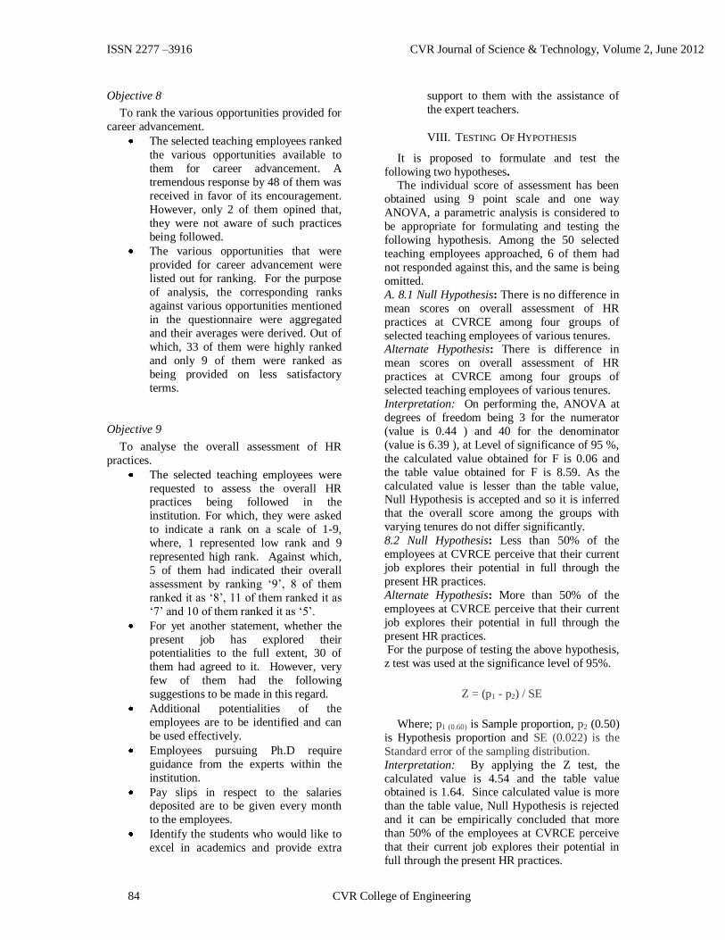
ISSN 2277 –3916 CVR Journal of Science & Technology, Volume 2, June 2012
Objective 8
To rank the various opportunities provided for
career advancement.
The selected teaching employees ranked
the various opportunities available to
them for career advancement. A
tremendous response by 48 of them was
received in favor of its encouragement.
However, only 2 of them opined that,
they were not aware of such practices
being followed.
The various opportunities that were
provided for career advancement were
listed out for ranking. For the purpose
of analysis, the corresponding ranks
against various opportunities mentioned
in the questionnaire were aggregated
and their averages were derived. Out of
which, 33 of them were highly ranked
and only 9 of them were ranked as
being provided on less satisfactory
terms.
Objective 9
To analyse the overall assessment of HR
practices.
The selected teaching employees were
requested to assess the overall HR practices being followed in the
institution. For which, they were asked
to indicate a rank on a scale of 1-9,
where, 1 represented low rank and 9
represented high rank. Against which,
5 of them had indicated their overall
assessment by ranking ‘9’, 8 of them
ranked it as ‘8’, 11 of them ranked it as
‘7’ and 10 of them ranked it as ‘5’.
For yet another statement, whether the
present job has explored their potentialities to the full extent, 30 of
them had agreed to it. However, very
few of them had the following
suggestions to be made in this regard.
Additional potentialities of the
employees are to be identified and can
be used effectively.
Employees pursuing Ph.D require
guidance from the experts within the
institution.
Pay slips in respect to the salaries deposited are to be given every month
to the employees.
Identify the students who would like to
excel in academics and provide extra
support to them with the assistance of
the expert teachers.
VIII. TESTING OF HYPOTHESIS
It is proposed to formulate and test the
following two hypotheses.
The individual score of assessment has been
obtained using 9 point scale and one way
ANOVA, a parametric analysis is considered to
be appropriate for formulating and testing the
following hypothesis. Among the 50 selected
teaching employees approached, 6 of them had
not responded against this, and the same is being
omitted.
A. 8.1 Null Hypothesis: There is no difference in
mean scores on overall assessment of HR
practices at CVRCE among four groups of
selected teaching employees of various tenures. Alternate Hypothesis: There is difference in
mean scores on overall assessment of HR
practices at CVRCE among four groups of
selected teaching employees of various tenures.
Interpretation: On performing the, ANOVA at
degrees of freedom being 3 for the numerator
(value is 0.44 ) and 40 for the denominator
(value is 6.39 ), at Level of significance of 95 %,
the calculated value obtained for F is 0.06 and
the table value obtained for F is 8.59. As the
calculated value is lesser than the table value, Null Hypothesis is accepted and so it is inferred
that the overall score among the groups with
varying tenures do not differ significantly.
8.2 Null Hypothesis: Less than 50% of the
employees at CVRCE perceive that their current
job explores their potential in full through the
present HR practices.
Alternate Hypothesis: More than 50% of the
employees at CVRCE perceive that their current
job explores their potential in full through the
present HR practices. For the purpose of testing the above hypothesis,
z test was used at the significance level of 95%.
Z = (p1 - p2) / SE
Where; p1 (0.60) is Sample proportion, p2 (0.50)
is Hypothesis proportion and SE (0.022) is the
Standard error of the sampling distribution.
Interpretation: By applying the Z test, the
calculated value is 4.54 and the table value obtained is 1.64. Since calculated value is more
than the table value, Null Hypothesis is rejected
and it can be empirically concluded that more
than 50% of the employees at CVRCE perceive
that their current job explores their potential in
full through the present HR practices.
84 CVR College of Engineering

ISSN 2277 –3916 CVR Journal of Science & Technology, Volume 2, June 2012
SUGGESTIONS AND CONCLUSIONS
The HR practices have a direct impact on the
employees of any educational institution. These
practices not only help the employees to grow in
an institutional stratum, but also serve as a mode for effective and qualitative teaching. Although,
most of the HR practices were well appreciated
by the selected teaching employees, it was also
found that there were some lacunae, which are
yet to be identified and improved for further
enhancement of the quality of HR practices.
The primary data collected from the study has
proved that the selected teaching employees of
CVRCE were contented with the various HR
practices provided to them and its subsequent
impact was also obvious from the various
achievements of CVRCE as inferred from the secondary data. The statistical tools applied to
various assumptions made in the study,
empirically concluded that the tenure of the
employees has impact on the perception of
overall assessment of HR practices at CVRCE
and it was also concluded that more than 50% of
the employees at CVRCE perceive that their
current job explores their potential in full
through the present HR practices.
In a nutshell, HR practices, in the cause of
education especially by an educational institution are imperative for the pursuit of excellence and
also for building up wise and skilled citizens of a
nation.
SCOPE FOR FURTHER STUDY
The measurement of HR practices followed by
an institution is a continuous process. Also, in
the context of enhancing and improving the HR
practices in future and with greater chances of
further increase in the size of the teaching
employees in the years ahead, there is a scope to
conduct similar study over a period of time.
ACKNOWLEDGEMENT
At the outset we wish to express our sincere
gratitude to the Management without whose kind
approval this study titled ‘HR Practices at
CVRCE’ would have never been possible. The
institutionalisation of good HR practices
commenced with the former Principal, Dr. Rama
Sastry, our present Director. We also thank our
Principal Dr. A.D. Rajkumar, for his kind
consideration in providing me an opportunity to
carry out the same. We also take this
opportunity in thanking all the teaching staff of the Department of Management Studies who
contributed with their valuable suggestions
during the Pilot survey. We also would like to
thank all the respondents of the study for their
kind cooperation, keen interest and timely
submission of the filled-in questionnaires. Our
sense of gratitude is conveyed in a special way to
all the Heads and Professors of various departments who were also part of the
respondents. We also owe our gratitude to Ms.
Harini, DTP operator, for rendering her
assistance in making the Questionnaires
available in the form of softcopy.
REFERENCES
[1] Guest, D (2002). Human Resource Management, Corporate Performance and Employee Wellbeing: Building the Worker into HRM, the Journal of Industrial Relations, 44(3), 335-358.
[2] Gould-Williams, J. (2003). The importance of HR practices a workplace trust in achieving superior performance: A study of public sector institutions, International Journal of Human Resource Management, 14(1), 28-54.
[3] Harley, B (2002). Employee Responses to High Work Performance System Practices,
the Journal of Industrial Relations, 44(3), 418-434.
[4] Park, H. J. Mitsuhashi, H.Fey, C.F.Bjorkman, I. (2003). The effect of human resource management practices on Japanese MNC subsidiary performance, 14(8), 1391-1406.
[5] Wright, P.M.Garden, T.M, T.M. and Moynihan, L.M. (2003). The impact of HR
practices on the performance of business units, Human Resource Management Journal, 13 (3), 21-36.
[6] Tessema, M and Soeters, J (2006). Challenges and prospects of HRM in developing countries: International Journal of Human Resource Management, 17(1), 86-105.
[7] http://cvr.ac.in [8] News letters, Brochures and Service manual
of CVRCE.
CVR College of Engineering 85

ISSN 2277 –3916 CVR Journal of Science & Technology, Volume 2, June 2012
Queuing Theory-A Tool For Optimizing
Hospital Services V.R.Girija
1 and Prof.M.S.Bhat
2
1 Deccan School of Management, Department of Hospital Maagement, Hyderabad, India
Email: [email protected] 2CVR College of Engineering, Department of Management Studies, Ibrahimpatan, R.R.District, A.P., India
Email: [email protected]
Abstract -Allocation of scarce resources presents an
increasing challenge to hospital administrators and
health policy makers. In health care situations, we
typically want to minimize cost or maximize quality or,
more likely, some combination of these two. Application
of queuing theory in hospital, attempts to improve the
delivery of patient care services in the outpatient
department as well as other departments. Calculation of
Traffic intensity with a mean waiting time & Service
timings helps to understand the congestion and
overcrowding in the system or to identify the service
facilities which are idle, thus leading to optimization of
resources.
This study analyzes the queuing characteristics in
tertiary and secondary care government hospitals in
twin cities of Hyderabad and Secunderabad. A sample
of 200 patients were randomly selected and observed to
understand their arrival and service patterns.
Surprisingly both the hospitals had very less utilization
rate (26.58% in tertiary care & 28.16% in secondary
care) and very high idle rate (73% in tertiary care &
71% in secondary care). The results clearly show that
the utilization rate is very small which needs attention
by the policy makers to improve the efficiency of the
system in both the government hospitals.
Index terms-queue, waiting line, optimization, arrival
rate, service rate.
I. INTRODUCTION
Easy access is one of the fundamental demands
placed on health services. Accessibility mainly in
relation to waiting times is the aspect with which
patients express greatest dissatisfaction. Although
healthcare is usually delivered within a reasonable
period, most people instinctively react to waiting
times in a negative way.
In many countries, the critical importance of this
issue prompted the rapid expansion of research on
waiting times and access to health services. The main
lines of research focus on theories to explain the causes of waiting times, analysis of the scope and
consequences of waiting times, and evaluations of
various initiatives aimed at correcting the problem.
One of the fundamental requirements on health
services is good access to health care. “Good access”
is defined as “the provision of care in relation to the
needs of citizens, irrespective of their geographical,
social or economic situation”. Waiting times are one
of the important aspects of access to health care.
Waiting times and access to health services can be viewed as health policy issues. They can be related to
the management and distribution of health care
resources and the public‟s consumption of health
services.
With the growing population & changing life style,
hospitals are getting crowded day by day. At the
same time patients who are sick, hesitate to wait for
longer periods in queue. Thus understanding the
Queue behavior and optimizing on the Waiting time,
Service cost as well as Idle resources is an important
task that every hospital should achieve to tackle the
needs of increased patient flow without making them wait for longer periods.
II. LITERATURE REVIEW
There has been some work on managing
hospital waiting lists and allocating beds in a hospital
to various services. One interesting aspect of health
care waiting lists is the dynamic nature of the
problem: as the queue increases, the reneging rate
increases. People on the list look for services else
where.
“Ref.[1]” analyzed and suggested the applications
of Queuing theory in healthcare organizations around the world. He suggested that Queuing theory can be
applied in health service capacity planning,
emergency room arrivals, walk in patients in
physician offices, outpatient clinics, outpatient
surgeries in hospitals, hospital pharmacy and
pharmacy stores, healthcare resource and
infrastructure planning for disaster management and
public health.
“Ref. [2]” reviews the use of Queuing theory in
pharmacy applications with particular attention to
86 CVR College of Engineering

ISSN 2277 –3916 CVR Journal of Science & Technology, Volume 2, June 2012
improving customer satisfaction. “Ref. [3]” presents
a brief history of the use of queuing theory in
healthcare and gives the extensive list of the
bibliography of the research works on queuing theory.
“Ref. [4]” discusses the application of Queuing in
healthcare with respect to delays, utilization and
number of servers. “Ref. [5]” analyses that increase
in service capacity ,doesn‟t affect the queue much -
as patient arrival rate increases - as and when they
feel that ,queue length is less.
III. OBJECTIVES OF THE STUDY
1. To study the waiting time distribution of patients
in the Out Patient department of a Tertiary and
Secondary care Government hospital. 2. To apply the Waiting Line model or Queuing
Theory as a tool for optimizing hospital services.
IV. MATERIALS AND METHODS
A. The data collection device
Data is collected with the help of a questionnaire
designed for finding patient expectations. Observation method is also used to find out the inter-
arrival times of patients.
B. The Sample
A sample of 200 Out-patients (OP) each is taken
from the secondary and tertiary government hospital.
The period of the study is for 1 month. The survey is conducted in the general OP. There is an average
daily general OP of 35 in the tertiary care and
average daily general OP of 40 in the Secondary care.
For 1 month the population is 1,050 patients in
tertiary care & 1200 in secondary care. Patients are
selected randomly to find the inter-arrival timings
and service timings.
C. Data collection Process
The data is collected through questionnaire method
and observation. The questionnaire was prepared to
find the patient expectations in the hospital which
addressed some questions on waiting time of patients.
D. Data Analysis and Results
In most of the Queuing situations customer arrival
is random i.e. the occurrence of an event is not
influenced by the length of time that has elapsed
since the occurrence of last event. Random inter-
arrival and service times are described quantitatively
in queuing models by the exponential distribution.
The cumulative probability distribution function of
Exponential distribution is given as in (1).
F (t) = 1-e- λt (1)
Where „λ‟ is the arrival rate, „e‟ = 2.71828 and„t‟
is time and t >= 0. In the present study chi-square test
of “Goodness of Fit” is used to test the following
hypotheses.
Hypotheses 1
Ho: Inter-arrival time at Out Patient Department of
tertiary care government hospital follows exponential
distribution.
H1: Inter-arrival time at Out Patient Department of
tertiary care government hospital does not follow
exponential distribution.
Hypotheses 2
Ho: Inter-arrival time at Out Patient Department of
secondary care government hospital follows
exponential distribution.
H1: Inter-arrival time at Out Patient Department of
secondary care government hospital does not follow exponential distribution.
Hypotheses 3
Ho: Service time at Out Patient Department of
tertiary care government hospital follows exponential
distribution.
H1: Service time at Out Patient Department of tertiary care government hospital does not follow
exponential distribution.
Hypotheses 4
Ho: Service time at Out Patient Department of
secondary care government hospital follows
exponential distribution. H1: Service time at Out Patient Department of
secondary care government hospital does not follow
exponential distribution.
The following tables show the inter-arrival times
and service times of patients for both the hospitals.
TABLE-I
ARRIVAL TIME DISTRIBUTION FOR TERTIARY CARE
GOVERNMENT HOSPITAL
Inter-
arrival
time
(minutes)
5-10
10-20
20-30
30-45
45-60
60-120
Observed
frequency (
O)
57
48
35
27
21
12
Expected
Frequency
( E)
49.97
37.48
35.83
29.2
20.77
20.38
As per “Table I" the mean inter-arrival rate is
26.0875 minutes. The arrival rate is (λ) is 2.3 patients
per hour. The calculated value of is 7.572. The
critical value of at 5 (6-1) degree of freedom for α = 5% level of significance is 11.070. Hence Ho
(Inter-arrival time at Out Patient Department of
tertiary care government hospital follows exponential
CVR College of Engineering 87

ISSN 2277 –3916 CVR Journal of Science & Technology, Volume 2, June 2012
distribution) in hypothesis 1 may be accepted, as
calculated value is less than critical value.
TABLE-II
ARRIVAL TIME DISTRIBUTION FOR SECONDARY CARE
GOVERNMENT HOSPITAL
Inter-
arrival
time
(minutes)
5-10
10-20
20-30
30-45
45-60
60-120
Observed
frequency
( O)
68
42
37
30
10
13
Expected
Frequency
( E)
49.97
37.48
35.83
29.2
20.77
20.38
As per “Table II” the mean inter-arrival rate is
24.425 minutes. The arrival rate is (λ) is 2.45 patients
per hour. The calculated value of is 10.989. The
critical value of at 5 (6-1) degree of freedom for α = 5% level of significance is 11.070. Hence Ho (Inter-arrival time at Out Patient Department of
secondary care government hospital follows
exponential distribution) in hypothesis 2 may be
accepted, as calculated value is less than critical
value.
TABLE- III
SERVICE TIME DISTRIBUTION FOR TERTIARY CARE GOVERNMENT
HOSPITAL
Service time
(minutes)
0-5
5-10
10-15
15-20
Observed
frequency ( O)
56
69
48
27
Expected
Frequency ( E)
50.2
65.76
36.9
20.7
As per “Table III” the mean service rate is 8.65
minutes. The service rate is (µ) is 6.936 patients per
hour. The calculated value of is 6.086. The
critical value of at 3 (4-1) degree of freedom for α = 5% level of significance is 7.815. Hence Ho
(Service time at Out Patient Department of tertiary
care government hospital follows exponential
distribution) in hypothesis 3 may be accepted, as
calculated value is less than critical value.
TABLE-IV
SERVICE TIME DISTRIBUTION FOR SECONDARY CARE
GOVERNMENT HOSPITAL
Service time
(minutes)
0-5
5-10
10-15
15-20
Observed frequency (
O)
59
70
42
31
Expected Frequency (
E)
49.95
65.59
36.92
20.78
The mean service rate is 8.7 minutes. The service
rate is (µ) is 6.896 patients per hour. The calculated
value of is 7.6604. The critical value of at 3 (4-1) degree of freedom for α = 5% level of
significance is 7.815. Hence Ho (Service time at Out Patient Department of secondary care government
hospital follows exponential distribution) in
hypothesis 4 may be accepted, as calculated value is
less than critical value.
From the above tables it is clear that inter-arrival
timings and service timings in both the hospitals are
following exponential distribution. With these
findings a single server queuing model is applied to
study the following queuing characteristics for both
the hospitals. Utilization parameter or traffic intensity
given by (2).
P= λ / µ (2)
Idle rate or the probability that there are no
customers in the system either in the queue or in the
service given by (3).
Po = 1-p (3)
Length of the system or the average number of
customers in the system or expected number of
customers in the system given by (4).
Ls = λ / (µ- λ) (4)
Length of the queue or the average number of
customers in the queue or expected number of
customers in the queue given (5).
Lq = λ2 / [µ (µ- λ)] (5)
Expected waiting time in the system or average
waiting time in the system given (6).
Ws = 1 / (µ- λ) (6)
Expected waiting time in the queue or Average
waiting time in the queue given by (7).
Wq = λ / [µ (µ- λ)] (7)
TABLE-V
QUEUING CHARACTERISTICS FOR TERTIARY AND SECONDARY
CARE HOSPITAL
Queue character Tertiary care
hospital ( minutes)
Secondary care
hospital (minutes)
λ 2.3 2.45
µ 8.65 8.7
P 0.2658 0.2816
Po 0.73 0.71
Ls 0.36 0.392
Lq 0.096 0.11
Ws 0.15 0.16
Wq 1.688 1.76
88 CVR College of Engineering

ISSN 2277 –3916 CVR Journal of Science & Technology, Volume 2, June 2012
From the above table it is clear that both the
hospitals are not differing much in their arrival and
service timings. In both the hospitals (73% in tertiary
care & 71% in secondary care) the system is idle for a longer period of time. This clearly shows that for
almost more than 70% of the time there are no
customers either in the queue or in the system.
Similarly the system is busy (26.58% in tertiary care
& 28.16% in secondary care) for less than 30% of the
time. It means that the system has more capacity and
can accommodate more patients in the given OP
timings. The average number of customers either in
the queue or in the system is not even one. Average
waiting time in the queue is more for patients in both
the hospitals (1.688 minutes in tertiary care and 1.76 minutes in secondary care) when compared to the
average waiting time in the system (0.15 minutes in
tertiary care & 0.16 minutes in secondary care).
The results clearly show that the utilization rate is
very small which needs attention by the policy
makers. The resources can be better utilized to
provide more care to the patients. May be opening
the clinics in the evening and on government
holidays may increase the patient flow and decrease
the idle rate. Conducting medical camps often also
increases patient flow.
CONCLUSION
Queuing theory helps to understand the different
aspects of patients waiting in the queue as well as in
the system. In both government hospitals the idle rate
is more. This may be because of the patients more
shifting for private healthcare. It is felt by patients
that private hospitals provide better quality care when
compared to government hospitals. Also insurance is
helping patients to pay the high costs of private
hospitals. At the same time private hospitals have
more facilities, infrastructure and maintenance when
compared to government hospitals. The study can be extended to private hospitals to
find the queuing characters in that hospital. The study
was conducted only in the Outpatient department of
both government hospitals. The study can be
extended to find the queuing characteristics in
emergency room arrivals, outpatient surgeries in
hospitals, hospital pharmacy and disaster
management as suggested by Reetu Mahendiratta1.
Queuing theory application plays an important role in
optimization of hospital services and increase the
patient satisfaction by reducing the queue length or providing more servers in case of long queues.
Similarly management can plan to optimally utilize
the resources in case of large idle rates.
REFERENCES
[1] Reetu mahandiratta, “Applications of Queuing theory in Health Care,” International Journal of computing and Business Research, vol. 2, issue 2, May 2011.
[2] R.A.Nosek, J.P.Wilson, “Queuing Theory and customer satisfaction: a review of terminology, trends and applications to pharmacy practice,”
Hospital Pharmacy 2001, PP 275-279. [3] J.Preater “Queues in health”, Healthcare
Management science, Vol. 5, PP283, 2002. [4] L.Green, “Queuing analysis in health care in
patient flow: Reducing delay in health care delivery,” Springer, NewYork, PP 281-308.
[5] D.J.Worthington, “Hospital waiting list management models,” The journal of operation
research society, Vol. 42, PP 833-843.
CVR College of Engineering 89

ISSN 2277 –3916 CVR Journal of Science & Technology, Volume 2, June 2012
Effect of Inflation On Various Commodities Lalitha Suddapally
CVR College of Engineering, Department of Management Studies, Ibrahimpatan, R.R.District, A.P., India
Email: [email protected].
Abstract - As we all know inflation rate refers to a general rise
in prices measured against a standard level of purchasing
power. This is discussed in the context of continuous rise of
prices. When there is inflation, currency loses its purchasing
power. This may be caused by either demand pull or cash
push. In India inflation is measured based on the Wholesale
Price Index (WPI), where as in developed countries like US,
they use Consumer Price Index (CPI) as the basis. Presently in
India, the index is calculated taking into account price levels
of 1100 items and the year 2004-05 as base year. Inflation
affects different categories of people in varying measures.
Prices of some goods and services rise faster than others,
where as for some goods and services, there may not be any
remarkable change. The poor and the middle class suffer a lot
because of continuous rise of prices as their wages and salaries
are almost fixed. On the other hand, people with variable
incomes benefit a lot out of it. In this paper it is attempted to
study the influence of inflation on various commodity prices to
understand how in real sense it is changing the consumption
function. In this analysis it is revealed surprisingly that the
prices of primary articles and food grains continually are
increasing irrespective of variations in inflation. It is well
known fact that for these basic needs only, major share of the
income of poor and middle class people is spent. This means a
continuous increase in burden on them. It is also observed that
some commodity prices are varying in line with inflation and
for some others no much variation is seen. From this study, it
is felt that there is an immediate attention required to change
the weight-ages given to various commodities in calculating
the inflation to reflect reality.
Index Terms – Inflation, Wholesale Price Index, Consumer
Price Index, Gross Domestic Product, commodity, needs,
consumption function, weight-ages.
I. INTRODUCTION
Inflation implies a general increase in the prices measured against a general level of the power to purchase.
The measure of inflation is obtained by comparing two sets
of goods at different times. When there is inflation, the
currency loses its purchasing power. For example, when
Rs. 20 is the price of rice, with Rs. 100 one can purchase 5
Kgs, if its price increases to Rs. 25 in the next period, with
the same Rs. 100 only 4 Kgs can be purchased. The
computing for the increase in the cost, which is not
reflected by increase in the quality, is carried out. There
may be two causes for inflation. One demand pull i.e.,
excessive demand for the product and other is cash push i.e., decrease in supply of goods and increase in cost of
factors of production. In India inflation is measured by the
Wholesale Price Index (WPI) but many developed
countries like UK, US, Japan and China, use the Consumer
Price Index (CPI) to calculate inflation. in India the Office
of the Economic Adviser to the Government undertook to
publish for the first time, an index number of wholesale
prices, with base week ended August 19, 1939 = 100, from
the week commencing January 10, 1942. The index was
calculated as the geometric mean of the price relatives of 23
commodities classified into four groups: (1) food &
tobacco; (2) agricultural commodities; (3) raw materials;
and (4) manufactured articles. The price index is an
indicator of the average price movement over time of a fixed basket of goods and services. . The WPI number is a
weekly measure of wholesale price movement for the
economy. WPI is based on Laspeyres formula. WPI is also
the price index which is available on a shortest possible
time lag i.e., two weeks. To ensure that the items in the
index basket are as best representatives as possible, efforts
are made to include all the important items transacted in the
economy during the base year. The importance of an item
in the free market will depend on its traded value during the
base year. The National Statistical Commission has
recommended that base year should be revised every five year and not later than ten years. The well known criteria
for the selection of base year are (a) a normal year which
is a year in which there are no abnormalities in the level of
production, trade and in the price level and price variations,
(b) a year for which reliable production, price and other
required data are available and (c) a year as recent possible
and comparable with other data series at national and state
level. The base year at present is 2004-05 and the index
calculation is based on 1,100 items instead of 435 used with
the base year 1993-94.
A. Calculation of WPI and Inflation Rate
Let's calculate WPI for the year 2015 for a particular
commodity, say rice. Assume that the price of a kilogram
of rice in 2005 = Rs 20.00 and in 2015 = Rs 40.00. The
WPI of rice for the year 2015 is, (Price of rice in 2015 –
Price of rise in 2005)/ Price of rice in 2005 x 100 = (40 –
20)/20 x 100 = 100. Since WPI for the base year is assumed as 100, WPI for 2015 will become 100 + 100 = 200. In this
way individual WPI values of the 1100 commodities are
calculated and then the weighted average of individual WPI
figures are found out to arrive at the overall WPI.
Commodities are given weight-age depending upon its
influence in the economy. The weight-ages that were given
90 CVR College of Engineering

ISSN 2277 –3916 CVR Journal of Science & Technology, Volume 2, June 2012
for primary commodities, fuel and ower and manufactured
products respectively are 20.12%, 14.91% and 64.97%.
Now, if we have the WPI values of two time zones, say,
beginning and end of year, the inflation rate for the year
will be, (WPI of end of year – WPI of beginning of
year)/WPI of beginning of year x 100. For example, WPI on Jan 1st 2015 is 200 and WPI of Jan 1st 2014 is 190 then
inflation rate for the year 2015 is,(200 – 190)/190 x 100 =
5.26% and we say the inflation rate for the year 2015 is
5.26%. This is how we get weekly inflation rates in India.
Likewise monthly and yearly inflation rates also can be
calculated [1].
B. Factors influencing inflation
When the government of a country print money in
excess, prices increase to keep up with the
increase in currency, leading to inflation.
Increase in production and labor costs, have a
direct impact on the price of the final product,
resulting in inflation.
When countries borrow money, they have to cope
with the interest burden. This interest burden
results in inflation.
High taxes on consumer products, can also lead to inflation.
Demands pull inflation, wherein the economy
demands more goods and services than what is
produced.
Cost push inflation or supply shock inflation,
wherein non availability of a commodity would
lead to increase in prices.
C. Problems with inflation
When the balance between supply and demand
goes out of control, consumers could change their
buying habits, forcing manufacturers to cut down
production.
The mortgage crisis of 2007 in USA could best
illustrate the ill effects of inflation. Housing prices
increased substantially from 2002 onwards,
resulting in a dramatic decrease in demand.
Inflation can create major problems in the economy. Price increase can worsen the poverty
affecting low income household,
Inflation creates economic uncertainty and is a
dampener to the investment climate slowing
growth and finally it reduces savings and thereby
consumption.
The producers would not be able to control the
cost of raw material and labor and hence the price
of the final product. This could result in less profit
or in some extreme case no profit, forcing them
out of business.
Manufacturers would not have an incentive to
invest in new equipment and new technology.
Uncertainty would force people to withdraw money from the bank and convert it into product
with long lasting value like gold, artifacts.
II. DISCUSSION AND ANALYSIS
Inflation affects people in varying measures. Prices of
some goods and services rise faster than others, where as
for some goods and services, there may not be any
remarkable change. The poor and the middle class suffer a
lot because of continuous rise of prices as their wages and
salaries are almost fixed. On the other hand, people with
variable incomes benefit a lot out of it. It changes the
consumption function.
A. Inflation trend in the last 4 years
Figure 1. Inflation (Y axis) for the last four years(X axis)
Inflation is observed to be very high from july, 2009 to
july, 2010. It is below 10 only in all other months [2].
TABLE I.
INFLATION FOR THE LAST FOUR YEARS
Year Jan Feb Mar Apr May June July Aug Sept Oct Nov Dec
2011 9.35 9.54 9.68 9.70 9.56 9.44 9.22 9.78 9.72 9.73 9.34 7.47
2010 16.22 14.86 14.86 13.33 13.91 13.73 11.25 9.88 9.82 9.70 8.33 9.47
2009 10.45 9.63 8.03 8.70 8.63 9.29 11.89 11.72 11.64 11.49 13.51 14.97
2008 5.51 5.47 7.87 7.81 7.75 7.69 8.33 9.02 9.77 10.45 10.45 9.70
CVR College of Engineering 91
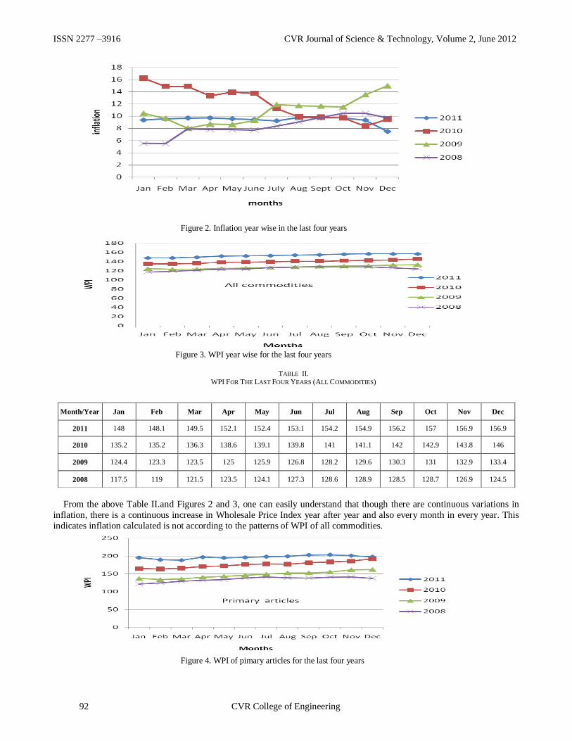
ISSN 2277 –3916 CVR Journal of Science & Technology, Volume 2, June 2012
Figure 2. Inflation year wise in the last four years
From the above Table II.and Figures 2 and 3, one can easily understand that though there are continuous variations in
inflation, there is a continuous increase in Wholesale Price Index year after year and also every month in every year. This
indicates inflation calculated is not according to the patterns of WPI of all commodities.
Month/Year Jan Feb Mar Apr May Jun Jul Aug Sep Oct Nov Dec
2011 148 148.1 149.5 152.1 152.4 153.1 154.2 154.9 156.2 157 156.9 156.9
2010 135.2 135.2 136.3 138.6 139.1 139.8 141 141.1 142 142.9 143.8 146
2009 124.4 123.3 123.5 125 125.9 126.8 128.2 129.6 130.3 131 132.9 133.4
2008 117.5 119 121.5 123.5 124.1 127.3 128.6 128.9 128.5 128.7 126.9 124.5
Figure 3. WPI year wise for the last four years
TABLE II. WPI FOR THE LAST FOUR YEARS (ALL COMMODITIES)
Figure 4. WPI of pimary articles for the last four years
92 CVR College of Engineering

ISSN 2277 –3916 CVR Journal of Science & Technology, Volume 2, June 2012
TABLE III.
WPI FOR THE LAST FOUR YEARS (PRIMARY ARTICLES)
Month/Year Jan Feb Mar Apr May Jun Jul Aug Sep Oct Nov Dec
2011 195.3 189.6 188.2 196.8 194.9 195.9 198.2 199.4 202.9 203.5 201.1 197.9
2010 164.9 163.6 165.9 171 172.6 176 177.8 177.3 180.8 183.4 185.3 192
2009 137.2 134.4 135.8 140.8 143.3 146.5 149.3 152.9 153 155.3 161.6 162.2
2008 121.2 124.8 128.9 132.1 134.2 138.3 141.1 139.2 138.3 140.8 141.4 137.5
TABLE IV.
WPI FOR THE LAST FOUR YEARS (FUEL AND POWER)
Month/Year Jan Feb Mar Apr May Jun Jul Aug Sep Oct Nov Dec
2011 151.3 153.5 157.6 159.5 160.4 161.6 165.6 167.1 168.3 170 171.6 172.6
2010 135.8 136.6 140.1 141.1 142.8 143.2 147.8 148 147.6 148.1 148.6 150.2
2009 127.2 124 123.1 124.2 124.8 125.7 130.5 131.5 132.9 133.4 134.7 135
2008 122.8 124 127.4 130.2 131.4 141.7 143.2 145.6 144.6 143.1 136.2 129.1
TABLE V.
WPI FOR THE LAST FOUR YEARS (MANUFACTURED PRODUCTS)
Month/Year Jan Feb Mar Apr May Jun Jul Aug Sep Oct Nov Dec
2011 132.6 134 135.6 136.6 137.4 137.9 138 138.4 139 139.6 139.8 140.6
2010 125.9 126.1 126.2 127.9 127.9 127.8 128.1 128.3 128.7 129.2 129.8 130.9
2009 119.8 119.7 119.8 120.2 120.8 121 121.1 122 122.6 122.9 123.6 124.2
2008 115.1 116 117.8 119.2 119.2 120.7 121.4 121.8 121.8 121.6 120.2 119.3
Figure 5. WPI of fuel and power for the last four years
CVR College of Engineering 93

ISSN 2277 –3916 CVR Journal of Science & Technology, Volume 2, June 2012
From the Tables II, III, IV and V, Figures 3, 4, 5 and 6,
we can observe that the pattern of all commodities which
are taken as a basis for the calculation of yearly inflation
almost resembles the pattern of manufactured products for
all the years. It may be because of the amount of weight-
age (64.97%) given to it. That means the total results are influenced by this weight-age of manufactured products 64,
97%.
The WPI of all commodities are ranging from 117.5 to
156.9 and manufactured products are ranging from 115,1 to
140.6 which are close to each other. Whereas when we
observe the primary articles and fuel & power, these values
are ranging from 121.2 to 197.9 and 122.8 to 172.6
respectively for the same period of time. This indicates the
rate of increase in prices of primary articles and fuel &
power is very high compared to that of manufactured
products. Further, the manufactured products are not letting the actual variation in the other two appear in the all
commodity WPI and also in inflation calculations as it has
major weight-age and is always below the other two.
As we all know, the primary articles include food articles
like rice, jowar, ragi, tea, coffee, urad, vegetables, fruits,
condiments, spices, mutton, chicken, pork, fish, egg,
buffalo meat, bajra, masur, gram, wheat, milk etc., Non-
food articles like gaur seed, flowers, linseed, soya bean,
rape and mustard seed, raw silk, sunflower and raw rubber,
safflower, groundnut seed, niger seed, gingelly seed,
fodder, cotton seed, castor seed, coir fiber, raw cotton and
raw jute etc., and minerals like sillimanite, barites, iron ore, bauxite, dolomite, crude petroleum, magnetite, steatite,
copper ore etc.
Fuel and power, include items such as electric power,
petrol, naphtha, aviation fuel, light diesel oil, diesel,
bitumen, furnace oil etc.
Manufactured products include food products like
processed prawn, canned fish, salt, gingelly oil, sugar,
mustard and rapeseed oil, groundnut oil, khandsari, palm
oil, powder milk, gaur, oil cakes, mixed spices, tea dust, tea
leaf, copra oil, wheat flour, ghee, beverages, coffee powder
etc., Other items of manufactured products include, tobacco and tobacco products, textiles, wood and wood products,
paper and paper products, leather and leather products,
chemicals and chemical products, non-metallic mineral
products, basic metals, alloys and metal products, transport
equipment and parts etc.
From the above, we can easily understand that the first
two categories are essential commodities and fulfill the
basic needs of the all human beings. Whereas the
manufactured products is mostly related to comforts and
luxuries related items, which are mostly consumed by
higher middle class and well to do class people. Though
primary articles and fuel & power are used by all the human beings, the amount of income spared for various
items in their consumption function vary from poor, lower
middle, higher middle and well to do class people. 70% -
90% of the income of poor and middle class people is
spared only for these two category items. Where as well to
do class people spare less than 10% of their income for
these two category of items. This means that when there is
greater rise in prices of these two categories of items, well
to do class has no much impact but the other two classes of
people have to sacrifice their other needs to fulfill these essential basic requirements as their income levels are
almost fixed.
In this regard, discussion about influence of rise of prices
on private sector and government employees also should be
done. Because, the income levels of private sector
employees are more or less fixed as there is no mechanism
in India to monitor the compensation for private sector
employees for inflation. This is very much true particularly
for poor and lower level employees of the private
organizations who amount to more than 60% of population.
For Government employees the Government announces DA to compensate the inflation influence on the cost of
living. This is also based on the calculated inflation rates
only which are not reflecting the reality because of more
weight-age to manufactured products. TABLE VI.
YEARLY WPI OF VARIOUS COMMODITIES FOR THE LAST
5 YEARS
Calendar Year 2010 2009 2008 2007 2006 2005
FOOD GRAINS
(CEREALS+PULSES) 174.13 160.31 141.13 129.18 118.71 104.28
Rice 165.87 154.21 135.58 118.68 107.79 104.43
Wheat 172.18 159.75 144.47 132.84 121.26 100.84
Pulses 200.84 178.8 151.35 147.83 141.99 106.63
Fruits and vegetables 163.02 143.61 131.93 124.12 108.38 106.11
Eggs, meat and fish 184.2 140.76 122.56 116.47 110.98 103.54
minerals 244.03 187.65 185.51 144.4 134.3 111.93
iron ore 504.81 271.78 299.59 194.15 163.17 113.86
LPG 121.7 112.34 115.24 106.1 106.1 106.1
Petrol 134.82 116.72 130.1 119.26 124.6 109.85
Electricity (Domestic) 113.23 107.38 104.88 103.73 100.87 99.18
Dairy products 150.38 132.99 121.02 114.75 102.58 99.4
sugar 166.36 145.64 99.14 92.63 110.49 107.6
Textiles 115.25 104.68 102.81 101.41 100.52 98.91
Paper 123.08 118.13 115.39 110.82 107.2 102.62
Fertilizers and Pesticides 114.02 108.26 107.03 106.02 104.28 101.81
Drugs and Medicines 114.5 112.32 110.99 106.46 102.22 100.91
cement 136.5 129.34 121.2 115.3 109.34 103.46
Steel and Alloys 142.95 136.66 137.11 121.01 109.88 105.55
Metal Products 160.9 147.89 141.51 123.65 117.02 104.1
Gold 275.78 228.3 188.08 150.07 142.84 102.27
Silver 285.54 202.04 192.88 171.83 155.13 101.01
Automotives 119.11 115.37 110.12 105.22 103.44 101.65
By-Cycles 134.1 131.93 119.63 114.67 109.44 103.72
And if we observe the trends of the very essential
commodities as given in the table 6, it is understood that
very essential commodities like food grains, rice, wheat,
pulses, vegetables, eggs, dairy products, sugar and by-
cycles which are consumed by poor and middle class by
Figure 6. WPI of Manufactured Products for the last four years
94 CVR College of Engineering

ISSN 2277 –3916 CVR Journal of Science & Technology, Volume 2, June 2012
sparing major share of their income have higher rate of
increase in their prices. But some goods like electricity,
petrol, textiles, LPG, paper, fertilizers and pesticides have
not that great increase but still almost at par with the
inflation rate calculated. Similarly items like iron ore,
minerals, cement, steel, metal products, gold. silver etc., which can indirectly influence the lives of many also have
higher rate of increase in price than the all commodity WPI.
That means the inflation rate calculated is not reflecting the
real time situation of the market. This is all because of not
giving proper weight-ages to the commodities and
commodity groups as per their real price variations in the
market. The present method of calculation of WPI and
inflation are mostly in favor of the rich because they are not
influenced by the increased prices of the essential
commodities much and at the same time they are
multiplying their money because investments, businesses and supportive policies mainly related to the manufactured
products. This is indirectly increasing the gap between the
rich and poor [3].
CONCLUSION
In this analysis, it is revealed surprisingly that though all
the commodity prices are continually increasing
irrespective of variations in inflation, the prices of primary
articles and food grains are continually increasing at quite
higher rate. This is not reflected by the WPI and inflation
measurement of the existing method. It is well known fact
that, for these basic needs only, major share of the income
of poor and middle class people is spent. This means a continuous increase in burden on them. It is also observed
that some commodity prices are varying in line with
inflation and for some others no much variation is seen.
From this study, it is felt that there is an immediate
attention required to change the weight-ages given to
various commodities in calculating the inflation to indicate
reality.
ACKNOWLEDGEMENTS
This paper is incomplete without my sincere thanks to
my husband, other family members, friends and teachers
who helped and co-operated to complete this work.
REFERENCES
[1] Amith Gosh, “Inflation in India: knowing the right numbers” – an article published in
http://knol.google.com/k/inflation%20india. [2] Publications of Planning Commission of India.
[3] Publications of Office of Economic Adviser, Govt. of India.
CVR College of Engineering 95

ISSN 2277 –3916 CVR Journal of Science & Technology, Volume 2, June 2012
NSL/ISSN/INF/2012/102 Date: 24.1.2012 Dr. A. D. Raj Kumar, CVR College of Engineering, Mangalpalli(V), Ibrahimpatan(M), Ranga Reddy, Hyderabad– 501510 Dear Sir/ Madam, We are happy to inform you that the following serial(s) published by you has been registered and assigned ISSN (Print) ISSN 2277 –3916 CVR Journal of Science and Technology
It is important that the ISSN should be printed on every issue preferably at the right hand top corner of the cover page. The Indian National Centre will be responsible for monitoring the use of ISSN assigned to Indian Serials and for supplying up to-date data of the same to the International Centre for ISSN, Paris. For this purpose we request you to send us the forth coming issue of your serial on complimentary basis. We solicit your co-operation in this regard. Yours sincerely
(V.V. Lakshmi) Head
National Science Library Please don’t forget to send a sample issue of the journal/URL with ISSN printed on it. Contact : Ms. Shobhna Vij e-mail : [email protected] phone : 011-26516672

ISSN 2277 –3916 CVR Journal of Science & Technology, Volume 2, June 2012