pathwise coordinate optimization - department of statistics

Pathwise Coordinate Optimization

Jerome Friedman∗

Trevor Hastie†

Holger Hofling‡

and Robert Tibshirani§

September 24, 2007

Abstract

We consider “one-at-a-time” coordinate-wise descent algorithmsfor a class of convex optimization problems. An algorithm of this kindhas been proposed for the L1-penalized regression (lasso) in the lter-ature, but it seems to have been largely ignored. Indeed, it seems thatcoordinate-wise algorithms are not often used in convex optimization.We show that this algorithm is very competitive with the well knownLARS (or homotopy) procedure in large lasso problems, and that itcan be applied to related methods such as the garotte and elastic net.It turns out that coordinate-wise descent does not work in the “fusedlasso” however, so we derive a generalized algorithm that yields thesolution in much less time that a standard convex optimizer. Finallywe generalize the procedure to the two-dimensional fused lasso, anddemonstrate its performance on some image smoothing problems.

Keywords and phrases: coordinate descent, lasso, convex optimization.

∗Dept. of Statistics, Stanford Univ., CA 94305, [email protected]†Depts. of Statistics, and Health, Research & Policy, Stanford Univ., CA 94305,

[email protected]‡Dept. of Statistics, Stanford Univ., CA 94305, [email protected]§Depts. of Health, Research & Policy, and Statistics, Stanford Univ, [email protected]

1

1 INTRODUCTION 2

1 Introduction

In this paper we consider statistical models that lead to convex optimizationproblems with inequality constraints. Typically, the optimization for theseproblems is carried out using a standard quadratic programming algorithm.The purpose of this paper is to explore “one-at-a-time” coordinate-wise de-scent algorithms for these problems. The equivalent of a coordinate descentalgorithm has been proposed for the L1-penalized regression (lasso) in theliterature, but it is not commonly used. Moreover, coordinate-wise algo-rithms seem too simple, and they are not often used in convex optimization,perhaps because they only work in specialized problems. We ourselves neverappreciated the value of coordinate descent methods for convex statisticalproblems before working on this paper.

In this paper we show that coordinate descent is very competitive withthe well known LARS (or homotopy) procedure in large lasso problems, candeliver a path of solutions efficiently, and can be applied to many otherconvex statistical problems such as the garotte and elastic net. We then goon to explore a non-separable problem in which coordinate-wise descent doesnot work— the “fused lasso”. We derive a generalized algorithm that yieldsthe solution in much less time that a standard convex optimizer. Finally wegeneralize the procedure to the two-dimensional fused lasso, and demonstrateits performance on some image smoothing problems.

A key point here: coordinate descent works so well in the class of problemsthat we consider because each coordinate minimization can be done quickly,and the relevant equations can be updated as we cycle through the variables.Furthermore, often the minimizers for many of the parameters don’t changeas we cycle through the variables, and hence the iterations are very fast.

Consider for example the lasso for regularized regression (Tibshirani 1996).We have predictors xij, j = 1, 2, . . . p, and outcome values yi for the ith ob-servation, for i = 1, 2, . . . n. Assume that the xij are standardized so that∑

i xij/n = 0,∑

i x2ij = 1. The lasso solves

minβ

1

2

n∑

i=1

(yi −p∑

j=1

xijβj)2

subject to

p∑

j=1

|βj| ≤ s. (1)

The bound s is a user-specified parameter, often chosen by a model selection

1 INTRODUCTION 3

procedure such as cross-validation. Equivalently, the solution to (1) alsominimizes the “Lagrange” version of the problem

f(β) =1

2

n∑

i=1

(yi −p∑

j=1

xijβj)2 + γ

p∑

j=1

|βj| (2)

where γ ≥ 0. There is a one-to-one correspondence between γ and the bounds — if β(γ) minimizes (2), then it also solves (1) with s =

∑pj=1 |βj(γ)|. In

the signal processing literature, the lasso and L1 penalization is known as“basis pursuit” (Chen et al. 1998).

There are efficient algorithms for solving this problem for all values of sor γ: see Efron et al. (2004), and the homotopy algorithm of Osborne et al.(2000). There is another, simpler algorithm for solving this problem for afixed value γ. It relies on solving a sequence of single-parameter problems,which are assumed to be simple to solve.

With a single predictor, the lasso solution is very simple, and is a soft-thresholded version (Donoho & Johnstone 1993) of the least squares estimateβ:

β lasso(γ) = S(β, γ) ≡ sign(β)(|β| − γ)+ (3)

=

β − γ if β > 0 and γ < |β|β + γ if β < 0 and γ < |β|0 if γ ≥ |β|.

(4)

This simple expression arises because the convex-optimization problem (2)reduces to a few special cases when there is a single predictor. Minimizing thecriterion (2) with a single standardized x and β simplifies to the equivalentproblem

minβ

1

2(β − β)2 + γ|β|, (5)

where β =∑

i xiyi is the simple least-squares coefficient. If β > 0, we candifferentiate (5) to get

df

dβ= β − β + γ = 0. (6)

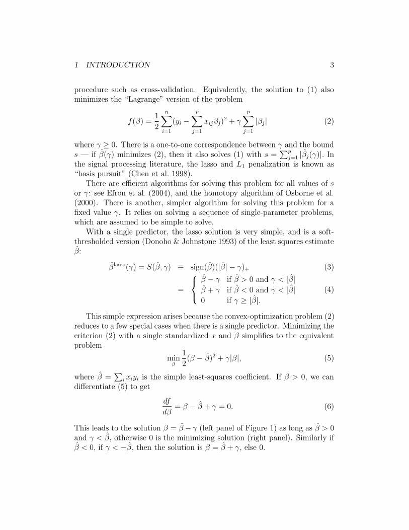
This leads to the solution β = β− γ (left panel of Figure 1) as long as β > 0and γ < β, otherwise 0 is the minimizing solution (right panel). Similarly ifβ < 0, if γ < −β, then the solution is β = β + γ, else 0.

1 INTRODUCTION 4

−1.0 −0.5 0.0 0.5 1.0 1.5 2.0

0.5

1.0

1.5

2.0

2.5

3.0

FA

LSE

−1.0 −0.5 0.0 0.5 1.0 1.5 2.0

PSfrag replacements

ββ

1 2(β−

β)2

+γ·|

β| β = 1.2, γ = 0.5 β = 1.2, γ = 1.3

Figure 1: The lasso problem with a single standardized predictor leads to softthresholding. In each case the solid vertical line indicates the lasso estimate, andthe broken line the least-squares estimate.

With multiple predictors that are uncorrelated, it is easily seen that onceagain the lasso solutions are soft-thresholded versions of the individual leastsquares estimates. This is not the case for general (correlated) predictors.Consider instead a simple iterative algorithm that applies soft-thresholdingwith a “partial residual” as a response variable. We write (2) as

f(β) =1

2

n∑

i=1

(yi −∑

k 6=j

xikβk − xijβj)2 + γ

∑

k 6=j

|βj|+ γ|βj|, (7)

where all the values of βk for k 6= j are held fixed at values βk(γ). Minimizingw.r.t. βj, we get

βj(γ) ← S(

n∑

i=1

xij(yi − y(j)i ), γ

)

(8)

where y(j)i =

∑

k 6=j xikβk(γ). This is simply the univariate regression coeffi-

cient of the partial residual yi− y(j)i on the (unit L2-norm) jth variable; hence

this has the same form as the univariate version (3) above. The update (7)is repeated for j = 1, 2, . . . , p, 1, 2, . . . until convergence.

An equivalent form of this update is

βj(γ) ← S(

βj(γ) +

n∑

i=1

xij(yi − yi), γ)

j = 1, 2, . . . p, 1, 2, . . . (9)

2 PATHWISE COORDINATEWISE OPTIMIZATION ALGORITHMS 5

0 5 10 15

020

040

060

0

Iteration

Coe

ffici

ent

2

3

4

7

9

1,5,6,8,10

Figure 2: Diabetes data: iterates for each coefficient from algorithm (9). Thealgorithm converges to the lasso estimates shown on the right side of the plot.

Starting with any values for βj, for example the univariate regression

coefficients, it can be shown that the βj(γ) values converge to β lasso.Figure 2 shows an example, using the diabetes data from Efron et al.

(2004). This data has 442 observations and 10 predictors. We applied al-gorithm (9) with γ = 88. It produces the iterates shown in the figure andconverged after 14 steps to the lasso solution β lasso(88).

This approach provides a simple but fast algorithm for solving the lasso,especially useful for large p. It was proposed in the “shooting” procedure ofFu (1998) and re-discovered by Daubechies et al. (2004). Application of thesame idea to the elastic net procedure (Zhou & Hastie 2005) was proposedby Van der Kooij (2007).

2 Pathwise coordinatewise optimization al-

gorithms

The procedure described in Section 1 is a successive coordinate-wise de-scent algorithm for minimizing the function f(β) = 1

2

∑

i(yi −∑

j xijβj)2 +

λ∑p

j=1 |βj|. The idea is to apply a coordinate-wise descent procedure for


each value of the regularization parameter, varying the regularization pa-rameter along a path. Each solution is used as a warm start for the nextproblem.

This approach is attractive whenever the single-parameter problem iseasy to solve. Some of these algorithms have already been proposed in theliterature, and we give appropriate references. Here are some other examples:

• The Non-negative garotte. This method, a precursor to the lasso, wasproposed by Breiman (1995) and solves

minc

1

2

n∑

i=1

(yi −p∑

j=1

xijcjβj)2 + λ

p∑

j=1

cj subject to cj ≥ 0. (10)

Here βj are the usual least squares estimates (we assume that p ≤ n).Using partial residuals as in (7), one can show that the the coordinate-wise update has the form

cj ←(

βjβj − λ

β2j

)

+

(11)

where βj =∑n

i=1 xij(yi − y(j)i ), and y

(j)i =

∑

k 6=j xikckβk.

• Least absolute deviation regression and LAD-lasso. Here the problemis

min β

n∑

i=1

|yi − β0 −p∑

j=1

xijβj|. (12)

We can write this asn∑

i=1

|xij|∣

∣

∣

(yi − y(j)i )

xij− βj

∣

∣

∣, (13)

holding all but βj fixed. This quantity is minimized over βj by a

weighted median of the values (yi − y(j)i )/xij. Hence coordinate-wise

minimization is just a repeated computation of medians. This approachis studied and refined by Li & Arce (2004).

The same approach may be used in the LAD-lasso (Wang et al. 2006).Here we add an L1 penalty to the least absolute deviation loss:

minβ

n∑

i=1

|yi − β0 −p∑

j=1

xijβj|+ λ

p∑

j=1

|βj| (14)


This can be converted into a LAD problem (12) by augmenting thedataset with p artificial observations. In detail, let X denote n×(p+1)model matrix (with the column of 1s for the intercept). The extra pobservations have response yi equal to zero, and predictor matrix equalto λ · (0 : Ip). Then the above coordinate-wise algorithm for the LADproblem can be applied.

• The Elastic net. This method, due to Zhou & Hastie (2005), adds asecond constraint

∑pj=1 β2

j ≤ s2 to the lasso (1). In Lagrange form, wesolve

minβ

1

2

n∑

i=1

(yi −n∑

j=1

xijβj)2 + λ1

p∑

j=1

|βj|+ λ2

p∑

j=1

β2j /2 (15)

The coordinate-wise update has the form

βj ←S(

∑ni=1 xij(yi − y

(j)i ), λ1

)

+

1 + λ2(16)

Thus we compute the simple least squares coefficient on the partialresidual, apply soft-thresholding to take care of the lasso penalty, andthen apply a proportional shrinkage for the ridge penalty. This algo-rithm was suggested by Van der Kooij (2007).

• Grouped Lasso (Yuan & Lin 2006). This is like the lasso, except vari-ables occur in groups (such as dummy variables for multi-level factors).Suppose Xj is an N × pj orthonormal matrix that represents the jthgroup of pj variables, j = 1, . . . , m, and βj the corresponding coefficientvector. The grouped lasso solves

minβ||y −

m∑

j=1

Xjβj||22 +m∑

j=1

λj||βj||2, (17)

where λj = λ√

pj. Other choices of λj ≥ 0 are possible; this one penal-izes large groups more heavily. Notice that the penalty is a weightedsum of L2 norms (not squared); this has the effect of selecting the vari-ables in groups. Yuan & Lin (2006) argue for a coordinate-descent al-gorithm for solving this problem, and show through the Karush-Kuhn-Tucker conditions that the coordinate updates are given by

βj ← (||Sj||2 − λj)+

Sj

||Sj||2, (18)


where Sj = XTj (y − y(j)), and here y(j)) =

∑

k 6=j Xkβk.

• The “Berhu” penalty. This method is due to Owen (2006), and isanother compromise between an L1 and L2 penalty. In Lagrange form,we solve

minβ

1

2

n∑

i=1

(yi−n∑

j=1

xijβj)2+λ

p∑

j=1

[

|βj|·I(|βj| < δ)+(β2

j + δ2)

2δ·I(|βj| ≥ δ)

]

.

(19)This penalty is the reverse of a “Huber” function—initially absolutevalue, but then blending into quadratic beyond δ from zero. Thecoordinate-wise update has the form

βj ←

S(∑n

i=1 xij(yi − y(j)), λ) if |βj| < δ∑n

i=1 xij(yi − y(j))/(1 + λ/δ) if |βj| ≥ δ(20)

This is a lasso-style soft-thresholding for values less than δ, and ridge-style beyond δ.

Tseng (1988) (see also Tseng (2001)) has established that coordinate de-scent works in problems like the above. He considers minimizing functionsof the form

f(β1, . . . βp) = g(β1, . . . βp) +

p∑

i=j

hj(βj) (21)

where g(·) is differentiable and convex, and the hj(·) are convex. Here eachβj can be a vector, but the different vectors cannot have any overlappingmembers. He shows that coordinate descent converges to the minimizer of f .The key to this result is the separability of the penalty function

∑pj=1 hj(βj),

a sum of functions of each individual parameter. This result implies that thecoordinate-wise algorithms for the lasso, the grouped lasso and elastic net,etc. converge to their optimal solutions.

Next we examine coordinate-wise descent in a more complicated problem,the “fused lasso” (Tibshirani et al. 2005), which we represent in Lagrangeform:

f(β) =1

2

n∑

i=1

(yi −p∑

j=1

xijβj)2 + λ1

p∑

j=1

|βj|+ λ2

p∑

j=2

|βj − βj−1|. (22)


0 200 400 600 800 1000

−2

02

4

genome order

log2

rat

io

0 200 400 600 800 1000

−2

02

4

genome orderlo

g2 r

atio

Figure 3: Fused lasso applied to some Glioblastoma Multiforme data. The dataare shown in the left panel, and the jagged line in the right panel represents theinferred copy number β from the fused lasso. The horizontal line is for y = 0.

The first penalty encourages sparsity in the coefficients; the second penaltyencourages sparsity in their differences; that is, flatness of the coefficientprofiles βj as a function of the index set j. Note that f(β) is strictly convex,and hence has a unique minimum.

The left panel of Figure 3 shows an example of an application of thefused lasso, in a special case where the feature matrix xij is the iden-tity matrix— this is called fused lasso signal approximation, discussed inthe next section. The data represents Comparative Genomic Hybridization(CGH) measurements from two Glioblastoma Multiforme (GBM) tumors.The measurements are “copy numbers”- log-ratios of the number of copiesof each gene in the tumor versus normal tissue. The data are displayed inthe left panel, and the red line in the right panel represents the smoothedsignal β from the fused lasso. The regions of non-zero estimated signal canbe used to call “gains” and “losses” of genes. Tibshirani & Wang (2007)report excellent results in the application of the fused lasso, finding that themethod outperforms other popular techniques for this problem.

Somewhat surprisingly, coordinate-wise descent does not work for thefused lasso. Proposition 2.7.1 of Bertsekas (1999), for example, shows that

2 PATHWISE COORDINATEWISE OPTIMIZATION ALGORITHMS10

every limit point of successive coordinate-wise minimization of a continuouslydifferentiable function is a stationary point for the overall minimization, pro-vided that the minimum is uniquely obtained along each coordinate. How-ever, f(β) is not continuously differentiable, which means that coordinate-wise descent can get stuck. Looking at Tseng’s result, the penalty functionfor the fused lasso is not separable, and hence Tseng’s theorem cannot beapplied in that case.

−1.0 −0.5 0.0

102.

010

2.5

103.

010

3.5

104.

0

−1.0 −0.5 0.0

102.

010

2.5

103.

010

3.5

104.

0

−1.0 −0.5 0.0−

1.0

−0.

50.

0

PSfrag replacements

β63β63

β64

β64

f(β

)

f(β

)

f(β)

Figure 4: Failure of coordinate-wise descent in a fused lasso problem with 100parameters. The optimal values for two of the parameters, β63 and β64, are both-1.05, as shown by the dot in the right panel. The left and middle panels showsslices of the objective function f(β) as a function of β63 and β64, with the otherparameters set to the global minimizers. The coordinate-wise minimizer over bothβ63 and β64 (separately) is -0.69, rather than -1.05. The right panel shows contoursof the two-dimensional surface. The coordinate-descent algorithm is stuck at (-0.69,-0.69). Despite being strictly convex, the surface has corners, in which thecoordinate-wise procedure can get stuck. In order to travel to the minimum wehave to move both β63 and β64 together.

Figure 4 illustrates the difficulty. We created a fused lasso problem with100 parameters, with the solutions for two of the parameters, β63 and β64 bothbeing equal to about -1. The top panels shows slices of the function f(β)varying β63 and β64, with the other parameters set to the global minimizers.We see that the coordinate-wise descent algorithm has got stuck in a cornerof the response surface, and is stationary under single-coordinate moves. Inorder to advance to the minimum, we have to move both β63 and β64 together.

3 THE FUSED LASSO SIGNAL APPROXIMATOR 11

Despite this, it turns out that the coordinate-wise descent procedure canbe modified to work for the fused lasso, yielding an algorithm that is muchfaster than a general quadratic-program solver for this problem.

3 The fused lasso signal approximator

Here we consider a variant of the fused lasso (22) for approximating one- andhigher-dimensional signals, which we call the fused-lasso signal approximator(FLSA). For one-dimensional signals we solve

minβ

f(β) =1

2

n∑

i=1

(yi − βi)2 + λ1

n∑

i=1

|βi|+ λ2

n∑

i=2

|βi − βi−1|. (23)

The measurements yi are made along a one-dimensional index i, and thereis one parameter per observation. Later we consider images as well. Inthe special case of λ1 = 0, the fused-lasso signal approximator is equivalentto a discrete version of the “total variation denoising” procedure (Rudinet al. 1992), used in signal processing. We make this connection clear inSection 6. Thus the algorithm that we present here also provides a fastimplementation for total variation denoising.

Figure 5 illustrates an example of FLSA with 1000 simulated data points,and the fit is shown for s1 = 269.2, s2 = 10.9.

We now describe a modified coordinate-wise algorithm for the diagonalfused lasso (FLSA) using the Lagrange form (23). The algorithm can alsobe extended to the general fused lasso problem; details are given in theAppendix. However it is not guaranteed to give the exact solution for thatproblem, as we later make clear.

Our algorithm, for a fixed value λ1, delivers a sequence of solutions cor-responding to an increasing sequence of values for λ2. First we make anobservation that makes it easy to obtain the solution over a grid of λ1 andλ2 values:

Proposition 1. The solutions to (23) for all (λ′1 > λ1, λ2) can be obtained

by soft-thresholding the solution for (λ1, λ2).

This is proven in the Appendix for the FLSA, two-dimensional penaltyfused lasso, and even more general penalty functionals. Thus our overallstrategy for obtaining the solution over a grid is to solve the problem for


0 200 400 600 800 1000

−2

−1

01

23

Index

Sig

nal

Figure 5: Fused lasso solution in a constructed example.

λ1 = 0 over a grid of values of λ2, and then use this result to obtain thesolution for all values of λ1. However for a single (especially large) valueof λ1, we demonstrate that is faster to obtain the solution directly for thatvalue of λ1 (Table 2). Hence we present our algorithm for fixed but arbitraryvalues of λ1.

Two keys for the algorithm are Assumptions (A1) and (A2) below, statingthat for fixed λ1, small increments in the value of λ2 can only cause pairsof parameters to fuse and they do not become unfused for larger of λ2 Thisallows us to efficiently solve the problem for a path of λ2 values, keeping λ1

fixed.The algorithm has three nested cycles:

Descent cycle: Here we run coordinate-wise descent for each parameter βj,holding all the others fixed.

Fusion cycle: Here we consider the fusion of a neighboring pair of parame-ters, followed by coordinate-wise descent.

Smoothing cycle: Here we increase the penalty λ2 a small amount, and rerunthe two previous cycles.

We now describe each in more detail.


1 2 3 4 5

−2

−1

01

Index

Y

−0.1 0.1 0.3 0.50.

120.

160.

20

0

−0.1 0.1 0.3 0.5

−0.

20−

0.10

0.00

0.10

Gra

dien

t

0

PSfrag replacements

β2β2

β3β3

β4β4

f(β

)

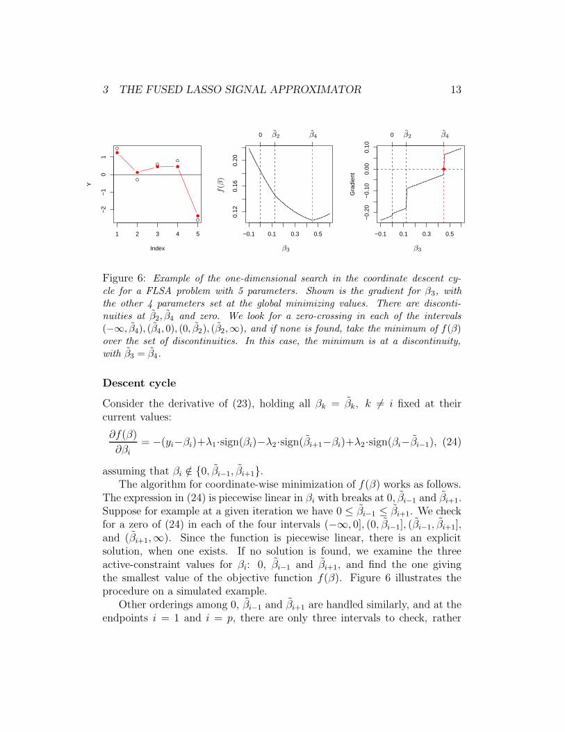
Figure 6: Example of the one-dimensional search in the coordinate descent cy-cle for a FLSA problem with 5 parameters. Shown is the gradient for β3, withthe other 4 parameters set at the global minimizing values. There are disconti-nuities at β2, β4 and zero. We look for a zero-crossing in each of the intervals(−∞, β4), (β4, 0), (0, β2), (β2,∞), and if none is found, take the minimum of f(β)over the set of discontinuities. In this case, the minimum is at a discontinuity,with β3 = β4.

Descent cycle

Consider the derivative of (23), holding all βk = βk, k 6= i fixed at theircurrent values:

∂f(β)

∂βi

= −(yi−βi)+λ1·sign(βi)−λ2·sign(βi+1−βi)+λ2·sign(βi−βi−1), (24)

assuming that βi /∈ 0, βi−1, βi+1.The algorithm for coordinate-wise minimization of f(β) works as follows.

The expression in (24) is piecewise linear in βi with breaks at 0, βi−1 and βi+1.Suppose for example at a given iteration we have 0 ≤ βi−1 ≤ βi+1. We checkfor a zero of (24) in each of the four intervals (−∞, 0], (0, βi−1], (βi−1, βi+1],and (βi+1,∞). Since the function is piecewise linear, there is an explicitsolution, when one exists. If no solution is found, we examine the threeactive-constraint values for βi: 0, βi−1 and βi+1, and find the one givingthe smallest value of the objective function f(β). Figure 6 illustrates theprocedure on a simulated example.

Other orderings among 0, βi−1 and βi+1 are handled similarly, and at theendpoints i = 1 and i = p, there are only three intervals to check, rather


than four.

Fusion cycle

The descent cycle moves parameters one at a time. Inspection of Figure 4shows that this approach can get stuck. One way to get around this is toconsider a potential fusion of parameters, when a move of a single βi failsto improve the loss criterion. This amounts to enforcing |βi − βi−1| = 0 bysetting βi = βi−1 = γ. With this constraint, we try a descent move in γ.Equation (24) now becomes

∂f(β)

∂γ= −(yi−1 − γ)− (yi − γ) (25)

+2λ1 · sign(γ)− λ2 · sign(βi+1 − γ) + λ2 · sign(γ − βi−2),

If the optimal value for γ decreases the criterion, we accept the move settingβi = βi−1 = γ.

Notice that the fusion step is equivalent to temporarily collapsing theproblem to one with p− 1 parameters:

• we replace the pair yi−1 and yi with the average response y = (yi−1 +yi)/2, and an observation weight of 2;

• the pair of parameters βi−1 and βi are replaced by a single γ, with apenalty weight of 2 for the first penalty.

At the end of the entire process of descent and fusion cycles for a givenλ2, we identify adjacent non-zero solution values that are equal and collapsethe data accordingly, maintaining a weight vector to assign weights to theobservations averages and the contributions to the first penalty.

Smoothing cycle

Although the fusion step often leads to a decrease in f(β), it is possibleto construct examples where for a particular value of λ2, no fusion of twoneighbors causes a decrease, but a fusion of three or more can. Our finalstrategy is to solve a series of fused lasso problems sequentially, fixing λ1,but varying λ2 through a range of values increasing in small increments δfrom 0.

The smoothing cycle is then as follows:


1. Start with λ2 = 0, hence with the lasso solution with penalty parameterλ1.

2. Increment λ2 ← λ2+δ, and run the descent and fusion cycles repeatedlyuntil no further changes occur. After convergence of the process for agiven value λ2, identify neighboring solution values that are equal andnon-zero and collapse the problem as described above, updating theweights.

3. Repeat step 2 until a target value of λ2 is reached (or a target bounds2).

Our strategy relies on the following assumptions:

A1. If the increments δ are sufficiently small, fusions will occur between nomore than two neighboring points at a time.

A2. Two parameters that are fused in the solution for (λ1, λ2) will be fusedfor all (λ1, λ

′2 > λ2)

By collapsing the data after each solution, we can achieve long fusions bya sequence of pairwise fusions. Note that each of the fused parameters canrepresent more than one parameter in the original problem. For example,if βj has a weight of 3, and βi+1 a weight of 2, then the merged parameterhas a weight of 5, and represents 5 neighboring parameters in the originalproblem.

After m fusions, the problem has the form

Cm + minβ

1

2

n−m∑

i=1

wi(yi − βi)2 + λ1

n−m∑

i=1

wi|βi|+n−m∑

i=2

|βi − βi−1|. (26)

Initially m = 0, wi = 1, and C0 = 0. If the (m + 1)st fusion is between βi−1

and βi, then the following updates occur:

• y ← (wi−1yi−1 + wiyi)/(wi−1 + wi),

• w+ ← wi−1 + wi,

• Cm+1 = Cm + 12[wi−1 · (yi−1 − y)2 + wi · (yi − y)2],

• yi−1 ← y, wi−1 ← w+,


2 4 6 8 10

01

23

45

2 4 6 8 10

01

23

45

2 4 6 8 10

01

23

45

2 4 6 8 10

01

23

45

PSfrag replacements

λ2 = 0 λ2 = 0.3

λ2 = 0.5 λ2 = 0.9

Figure 7: Small example of the fused lasso. λ1 is fixed at 0.01; as λ2 increases,the number of fused parameters increases.

• Discard observation i, and reduce all indices greater than i by 1.

Note that we don’t actually need to carry out the update for Cm, because noparameters are involved.

Figure 7 shows an example with just 9 data points. We have fixed λ1 =0.01 and show the solutions for four values of λ2. As λ2 increases, the numberof fused parameters increases.

Assumption A1 requires that the data have some randomness (i.e. nopre-existing flat plateaus exist). Assumption A2 holds in general. We provethat both assumptions hold for the FLSA procedure in the next section.

Numerical experiments show that A2 does not always hold for the generalfused lasso. Hence the extension of this algorithm to the general fused lasso(detailed in the Appendix) is not guaranteed to yield the exact solution. Notethat each descent and fusion cycle can only decrease the convex objective and

4 OPTIMALITY CONDITIONS 17

hence must converge. We terminate this pair of cycles when then change inparameter estimates is less than some threshold. The smoothing cycle isdone over a discrete grid of λ2 values.

4 Optimality conditions

In this section we derive the optimality conditions for the FLSA problem,and use them to show that our algorithms’s assumptions (A1) and (A2) aresatisfied.

We consider the Lagrangian form (23) for the fused lasso. The standardKarush-Kuhn-Tucker conditions for this problem are fairly complicated, sincewe need to express each parameter in terms of its positive and negative partsin order to make the penalty differentiable. A more convenient formulation isthrough the sub-gradient approach (see e.g. Bertsekas (1999), Prop. B.24).The equations for the subgradient have the form

−(y1 − β1) + λ1s1 − λ2t2 = 0

−(yj − βj) + λ1sj + λ2(tj − tj+1) = 0, j = 2, . . . n (27)

with sj = sign(βj) if βj 6= 0 and sj ∈ [−1, 1] if βj = 0. Similarly, tj =sign(βj − βj−1) if βj 6= βj−1 and tj ∈ [−1, 1] if βj = βj−1. These n equationsare necessary and sufficient for the solution. We restate assumptions (A1)and (A2) more precisely, and then prove they hold.

Proposition 2. For the fused-lasso signal approximation algorithm detailedin Section 3:

A1’. If the sequence yi are in general position— specifically, no two consec-utive yj values are equal— and the increments δ are sufficiently small,fusions will occur between no more than two neighboring points at atime.

A2’. Two parameters that are fused in the solution for (λ1, λ2) will be fusedfor all (λ1, λ

′2 > λ2)

Proof. We first prove (A2’). Suppose we have a stretch of nonzero solutions

βj−k, βj−k+1, . . . , βj that are equal for some value λ2, and βj−k−1 and βj+1

are not equal to this common value. Then tj−k and tj+1 each take a value in−1, 1; we denote these boundary values by Tj−k and Tj+1. Although the

4 OPTIMALITY CONDITIONS 18

parameters tj−k+1, . . . , tj can vary in [−1, 1] as λ2 changes (while the fusedgroup remains intact), the values depend only the (j − k + 1)th through jthequations in the system (27), because the boundary values are fixed. Taking

pairwise differences, and using the fact that βj−k = βj−k+1 = . . . = βj, thissubgroup of equations simplifies to

2 −1 0 0 · · · 0−1 2 −1 0 · · · 0...

......

.... . .

...0 0 · · · −1 2 −10 0 · · · 0 −1 2

tj−k+1

tj−k+2...

tj−1

tj

=1

λ2

yj−k+1 − yj+k

yj−k+2 − yj−k+1...

yj−1 − yj−2

yj − yj−1

+

Tj−k

0...0

Tj+1

(28)

Write this system symbolically as Mt = 1λ2

∆y + T , and let C = M−1. Theexplicit form for C given in Schlegel (1970) gives C`1 = (n − ` + 1)/(n +1), C`n = `/(n + 1). It is easy to check for all three possibilities for T thatCT ∈ [−1, 1] elementwise. We know that t = ( 1

λ2

C∆y + CT ) ∈ [−1, 1]elementwise as well, since t is a solution to (23) at λ2. For λ′

2 > λ2, theelements of the first terms shrink, and hence the values t(λ′

2) remain in[−1, 1]. This implies that the fused set remains fused as we increase λ2.These equations describe the path t(λ2) for λ2 increasing, and only changewhen one of the boundary points (fused sets) is fused with the current set,and the argument is repeated. This proves (A2’).

We now address (A1’). Suppose the data are in general position (e.g.have a random noise component), and we have the lasso-solution βj for λ1.

Because of the randomness, no neighboring non-zero parameters βj will be

exactly the same. This means for each nonzero value βj, we can write anequation of the form (27) where we know exactly the values for sj, tj and tj+1

(each will be one of the values −1, +1). This means that we can calculateexactly the path of each such βj as we increase λ2 from zero, until an eventoccurs that changes the sj, tj. By looking at all pairs, we can identify thetime of the first fusion of such pairs. The data are then fused together andreduced, and the problem is repeated. Fusions occur one-at-a-time in thisfashion, at a distinct sequence of values for λ2. Hence for δ small enough inour smoothing step, we can ensure that we encounter these fusions one at atime.

5 COMPARISON OF RUN TIMES 19

5 Comparison of run times

In this section we compare the run times of the coordinate-wise algorithmto standard algorithms, for both the lasso and diagonal fused lasso (FLSA)problems. All timings were carried out on a Intel Xeon 2.80GH processor.

5.1 Lasso speed trials

We generated Gaussian data with n observations and p predictors, with eachpair of predictors Xj, Xj′ having the same population correlation ρ. We trieda number of combinations of n and p, with ρ varying from zero to 0.95. Theoutcome values were generated by

Y =

p∑

j=1

βjXj + k · Z (29)

where βj = (−1)j exp(−2(j − 1)/20), Z ∼ N(0, 1) and k is chosen so thatthe signal-to-noise ratio is 3.0. The coefficients are constructed to have al-ternating signs and to be exponentially decreasing.

Table 1 shows the average CPU timings for the coordinatewise algorithm,two versions of the LARS procedure and lasso2, an implementation of thehomotopy algorithm of Osborne et al. (2000). All algorithms are imple-mented as R language functions. The coordinate-wise algorithm does all ofits numerical work in Fortran, while lasso2 does its numerical work in C.LARS-R is the “production version” of LARS (written by Efron and Hastie),doing much of its work in R, calling Fortran routines for some matrix op-erations. LARS-Fort (due to Ji Zhu) is a version of LARS that does all ofits numerical work in Fortran. Comparisons between different programs arealways tricky: in particular the LARS procedure computes the entire path ofsolutions, while the coordinate-wise procedure and lasso2 solve the problemsfor a set of pre-defined points along the solution path. In the orthogonal case,LARS takes min(n, p) steps: hence to make things roughly comparable, wecalled the latter two algorithms to solve a total of min(n, p) problems alongthe path.

Not surprisingly, the coordinate-wise algorithm is fastest when the cor-relations are small, and gets slower when they are large. It seems to bevery competitive with the other two algorithms in general, and offers somepotential speedup, especially when n > p.


Method Population correlation between features

n = 100, p = 10000 0.1 0.2 0.5 0.9 0.95

coord-Fort 0.31 0.33 0.40 0.57 1.20 1.45LARS-R 2.18 2.46 2.14 2.45 2.37 2.10LARS-Fort 2.01 2.09 2.12 1.947 2.50 2.22lasso2-C 2.42 2.16 2.39 2.18 2.01 2.71

n = 100, p = 50000 0.1 0.2 0.5 0.9 0.95

coord-Fort 4.66 4.51 3.14 5.77 4.44 5.43LARS-R 28.40 27.34 24.40 22.32 22.16 22.75LARS-Fort would not runlasso2 would not run

n = 100, p = 20, 0000 0.1 0.2 0.5 0.9 0.95

coord-Fort 7.03 9.34 8.83 10.62 27.46 40.37LARS-R 116.26 122.39 121.48 104.17 100.30 107.29LARS-Fort would not runlasso2 would not run

n = 1000, p = 1000 0.1 0.2 0.5 0.9 0.95


n = 5000, p = 1000 0.1 0.2 0.5 0.9 0.95


Table 1: Run times (CPU seconds) for lasso problems of various sizes n, p anddifferent correlation between the features. Methods are the coordinate-wise opti-mization (Fortran), LARS (R and Fortran versions) and lasso2 (C language)—the homotopy procedure of Osborne et al. (2000).


Figure 8 shows the CPU times for coordinate descent, for the same prob-lem as in Table 1. We varied n and p, and averaged the times over five runs.We see that the times are roughly linear in n and in p.

500 1000 1500 2000

01

23

45

6

Sample size n

CP

U s

econ

ds

500 1000 1500 2000

02

46

8

Number of predictors p

CP

U s

econ

ds

Figure 8: CPU times for coordinate descent, for the same problem as in Table 1,for different values of n and p. In each case the times are averaged over five runsand averaged over the set of values of the other parameter (n or p).

A key to the success of the coordinate-wise algorithm for lasso is the factthat, for squared error loss, the ingredients needed for each coordinate stepcan be easily updated as the algorithm proceeds. We can write the secondterm in (9) as

n∑

i=1

xij(yi − yi) = 〈xj, y〉 −∑

k:βk>0

〈xj, xk〉βk, (30)

where 〈xj, y〉 =∑n

i=1 xijyi, and so on. Hence we need to compute innerproducts of each feature with y initially, and then each time a feature xk

enters the model, we need to compute its inner product with all the rest.But importantly, O(n) calculations do not have to be made at every step.This is the case for all penalized procedures with squared error loss.

Friedlander & Saunders (2007) do a thorough comparison of the LARS(homotopy) procedure to a number of interior point QP procedures for thelasso problem, and find that LARS is generally much faster. Our finding


n = 1000λ1 λ2 # Active Coord Standard

0.00 0.01 456 0.040 2.1000.00 1.00 934 0.024 0.9310.00 2.00 958 0.019 0.9871.00 0.01 824 0.022 1.5191.00 1.00 975 0.024 1.5611.00 2.00 981 0.023 1.4042.00 0.01 861 0.023 1.4992.00 1.00 983 0.023 1.4182.00 2.00 991 0.018 1.407

n = 5000λ1 λ2 # Active Coord Standard

0.000 0.002 4063 0.217 20.6890.000 0.200 3787 0.170 26.1950.000 0.400 4121 0.135 29.1920.200 0.002 4305 0.150 41.1050.200 0.200 4449 0.141 48.9980.200 0.400 4701 0.129 45.1360.400 0.002 4301 0.108 41.0620.400 0.200 4540 0.123 41.7550.400 0.400 4722 0.119 38.896

Table 2: Run times (CPU seconds) for fused lasso (FLSA) problems of varioussizes n for different values of the regularization parameters λ1, λ2. The methodscompared are the pathwise coordinate optimization, and “standard”- two-phase ac-tive set algorithm sqopt of Gill et al. (1999). The number of active constraints inthe solution is shown in each case.


that coordinate descent is very competitive with LARS therefore suggeststhat also will outperform interior point methods.

Finally, note that there is another approach to solving the FLSA problemfor λ1 = 0. We can transform to parameters θj = βj−βj−1, and we get a newlasso problem in these new parameters. One can use coordinate descent tosolve this lasso problem, and then Proposition 1 gives the FLSA solution forother values of λ1. However this new lasso problem has a dense data matrix,and hence the coordinate descent procedure is many times slower than theprocedure described in this section. The procedure developed here exploitsthe near-diagonal structure of the problem in the original parametrization.

5.2 Fused lasso speed trials

For the example of Figure 5, we compared the pathwise coordinate algorithmto the two-phase active set algorithm sqopt of Gill et al. (1999). Bothalgorithms are implemented as R functions but do all but the setup andwrapup computations in Fortran. Table 2 shows the timings for the twoalgorithms for a range of values of λ1 and λ2. The resulting number of activeconstraints (i.e. βj = 0 or βj−βj−1 = 0) is also shown. In the second part ofthe table, we increased the sample size to 5000. We see that the coordinatealgorithm offers substantial speedups, by factors of 50 up to 300 or more.

In these tables, each entry for the pathwise coordinate procedure is thecomputation time for the entire path of solutions leading to the given valuesλ1, λ2. In practice, one could obtain all of the solutions for a given λ1 from asingle run of the algorithm, and hence the numbers in the table are very con-servative. But we reported the results in this way, to make a fair comparisonwith the standard procedure since it can also exploit warm starts.

n Average CPU sec

100,000 3.54500,000 14.931,000,000 29.81

Table 3: Run times (CPU seconds) for pathwise coordinate optimization appliedto fused lasso (FLSA) problems with a large number of parameters n averaged overdifferent values of the regularization parameters λ1, λ2.

6 THE TWO-DIMENSIONAL FUSED LASSO 24

In Table 3 we show the run times for pathwise coordinate optimization forlarger values of n. As in the previous table, these are the averages of run timesfor the entire path of solutions for a given λ1, and hence are conservative.We were unable to run the standard algorithm for these cases.

6 The two-dimensional fused lasso

Suppose we have total of n2 cells, laid out in a n × n grid (the square gridis not essential). We can generalize the diagonal fused lasso (FLSA) to two-dimensions as follows:

minβ

1

2

n∑

i=1

n∑

i′=1

(yii′ − βii′)2 (31)

subject ton∑

i=1

n∑

i′=1

|βii′ | ≤ s1,

n∑

i=1

n∑

i′=2

|βi,i′ − βi,i′−1| ≤ s2,

n∑

i=2

n∑

i′=1

|βi,i′ − βi−1,i′| ≤ s3.

The penalties encourage the parameter map βii′ to be both sparse and spa-tially smooth.

The fused lasso is related to signal processing methods such as “totalvariation denoising” (Rudin et al. 1992), which uses a continuous smoothnesspenalty analogous to the second penalty in the fused lasso. The TV criterionis written in the form

minu

∫

Ω

|∇u|du subject to ||u− y||2 = σ2 (32)

where y is the data, u is the approximation with allowable error σ2, Ω is abounded convex region in Rd, | · | denotes Euclidean norm in Rd and || · ||denotes the norm on L2(Ω). Thus in d = 1 dimension, this is a continuousanalogue of the fused lasso, but without the (first) L1 penalty on the coef-ficients. In d = 2 dimensions, the TV approach is different: the discretizedversion uses the Euclidean norm of the first differences in u, rather than thesum of the absolute values of the first differences.


This problem (32) can be solved by a general purpose quadratic-programmingalgorithm; we give details in the Appendix. However for a p× p grid, thereare 7p2 variables and 3p2 + 3 constraints, in addition to non-negativity con-straints on the variables. For p = 256 for example, this is 458, 752 variablesand 196, 611 constraints, so that finding the exact solution is impractical.

Hence we focus on the pathwise coordinate algorithm. The algorithmhas the same form as in the one-dimensional case, except that rather thanchecking the three active constraint values 0, βj−1 and βj+1, we check 0 andthe four values to the right, left, above and below (its four-neighborhood).The number of constraint values reduces to 4 at the edges and 3 at the cor-ners. The algorithm starts with individual pixels as the groups, and thefour-neighborhood pixels are its “distance-1 neighbors”. In each fusion cyclewe try to fuse a group with its distance-1 neighbors. If the fusion is ac-cepted, then the distance-1 neighbors of the fused group are the union of thedistance-1 neighbors of the two groups being joined (with the groups them-selves removed). Now one pixel might be the distance-1 neighbor to eachof the two groups being fused, and some careful bookkeeping is required tokeep track of this through appropriate weights. Full details are given in theAppendix.

We do not provide a proof of the correctness of this procedure. However,in our (limited) experiments we have found that it gives the exact solution tothe two-dimensional fused lasso. We guess that a proof along the lines of thatin the one-dimensional case can be constructed, although some additionalassumptions may be required.

As in the one-dimensional FLSA (Proposition 1), if we write the problemin terms of Lagrange multipliers (λ1, λ2, λ3), the solution for (λ′

1 > λ1, λ2, λ3)can be obtained by soft-thresholding the solutions for (λ1, λ2, λ3).

6.1 Example 1

Figure 9 shows a toy example. The data are in the top left, representinga “+”-shaped image with N(0, 1) noise added. The reconstruction by thelasso and fused lasso are shown in the other panels. In each case we did agrid search over the tuning parameters using a kind of two-fold validation.We created a training set of the odd pixels (1, 3, 5 . . . in each direction) andtested it on the even pixels. For illustration only, we chose the values thatminimized the squared reconstruction error over the test set. We see that thefused lasso has successfully exploited the spatial smoothness and provided a


0.0 0.2 0.4 0.6 0.8 1.0

0.0

0.2

0.4

0.6

0.8

1.0

Data

0.0 0.2 0.4 0.6 0.8 1.0

0.0

0.2

0.4

0.6

0.8

1.0

Lasso

0.0 0.2 0.4 0.6 0.8 1.0

0.0

0.2

0.4

0.6

0.8

1.0

Fused Lasso

Figure 9: A toy example: the data are in the top left, representing a “+”-shapedimage with added noise. The reconstruction by the lasso and fused lasso are shownin the other panels. In each case we did a grid search over the tuning parametersusing a kind of two-fold validation.


n Standard Coord8 2.0s 0.07s16 3.4s 0.13s32 20.8s 0.38s256 38m 7.1s

Table 4: 2D fused lasso applied to the toy problem. The table shows the number ofCPU seconds required for the standard and pathwise coordinate descent algorithms,as n increases. The regularization parameters were set at the values that yieldedthe solution in the bottom left panel of Figure 9.

much better reconstruction than the lasso.Table 4 shows the number of CPU seconds required for the standard and

pathwise coordinate descent algorithms, as n increases. We were unable toapply the standard algorithm for n = 256 (due to memory requirements),and have instead estimated the time by crude quadratic extrapolation.

6.2 Example 2

Figure 10 shows another example. The noiseless image (top panel) was ran-domly generated with 512×512 pixels. The background pixels are zero, whilethe signal blocks have constant values randomly chosen between 1 and 4. Thetop right panel shows the reconstruction by the fused lasso: as expected, itis perfect. In the bottom left we have added Gaussian noise with standarddeviation 1.5. The reconstruction by the fused lasso is shown in the bottomright panel, using two-fold validation to estimate λ1, λ2. The reconstructionis still quite good, capturing most of the important features. In this examplewe did a search over 10 λ1 values. The entire computation for the bottomright panel of Figure 10, including the two-fold validation to estimate theoptimal values for λ1 and λ2, took 11.3 CPU minutes.

6.3 Example 3.

The top left panel of Figure 11 shows a 256×256 gray scale image of statisti-cian Sir Ronald Fisher. In the top right we have added Gaussian noise witha standard deviation 2.5. We explore the use of the two-dimensional fusedlasso for denoising this image. However the first (lasso) penalty doesn’t make


Original image Fused lasso reconstruction

Noisy image Fused lasso reconstruction

Figure 10: A second toy example. The 100 × 100 noiseless and noisy images areshown on the left, while the corresponding fused lasso reconstructions are shownon the right. In each case we did a grid search over the tuning parameters λ1, λ2

using a kind of two-fold validation.

7 DISCUSSION 29

sense here as zero does not represent a natural baseline. So instead we trieda pure fusion model, with λ1 = 0. We found the best value of λ2, in terms ofreconstruction error from the original noiseless image. The solution shownin the bottom right panel, gives a reasonable approximation to the originalimage and reduces the reconstruction error from 6.18 to 1.15. In the bottomleft panel we have set λ2 = 0, and optimized over λ1. As expected, this purelasso solution does poorly, and the optimal value of λ1 turned out to be 0.

6.4 Applications to higher dimensions and other prob-

lems

The general strategy for the two-dimensional fused lasso can be directlyapplied in higher dimensional problems, the difference being that each cellwould have more potential distance-1 neighbors. In fact, the same strategymight be applicable to non-Euclidean problems. All one needs is a notionof distance-1 neighbors and the property that the distance-1 neighbors of afusion of two groups are the union of the distance-1 neighbors of the twogroups, less the fused group members themselves.

7 Discussion

Coordinate-wise descent algorithms deserve more attention in convex op-timization. They are simple and well-suited to large problems. We havefound that for the lasso, coordinate-wise descent is very competitive with theLARS algorithm, probably the fastest procedure for that problem to-date.Coordinate-wise descent algorithms can be applied to problems in which theconstraints decouple, and a generalized version of coordinate-wise descentlike the one presented here can handle problems in which each parameter isinvolved in only a limited number of constraints. This procedure is ideallysuited for a special case of the fused lasso— the fused lasso signal approxima-tor, and runs many times faster than a standard convex optimizer. On theother hand, it is not guaranteed to work for the general fused lasso problem,as it can get stuck away from the solution.

7 DISCUSSION 30

original image noisy image

lasso denoising fusion denoising

Figure 11: Top-left panel: 256 × 256 gray scale image of statistician Sir RonaldFisher. Top-right panel: Gaussian noise with standard deviation 2.5 has beenadded. Bottom-left panel: best solution with λ2 set to zero (pure lasso penalty); thisgives no improvement in reconstruction error. Bottom-right panel: best solutionwith λ1 set to zero (pure fusion penalty). This reduces the reconstruction errorfrom 6.18 to 1.15.

7 DISCUSSION 31

7.0.1 Software

Both Fortran and R language routines for the lasso, and the one- and two-dimensional fused lasso will be made freely available.

Acknowledgments

We thank Anita van der Kooij for informing us about her work on the elas-tic net, Michael Saunders and Guenther Walther for helpful discussions, andBalasubramanian Narasimhan for valuable help with our software. A specialthanks Stephen Boyd for telling us about the subgradient form (28). Whilewriting this paper, we learned of concurrent, independent work on coordi-nate optimization for the lasso and other convex problems by Ken Langeand Tongtong Wu. We thank the editors and two referees for commentsled to substantial improvements in the manuscript. Friedman was partiallysupported by grant DMS-97-64431 from the National Science Foundation.Hastie was partially supported by grant DMS-0505676 from the NationalScience Foundation, and grant 2R01 CA 72028-07 from the National Insti-tutes of Health. Hofling was supported by an Albion Walter Hewlett StanfordGraduate Fellowship. Tibshirani was partially supported by National ScienceFoundation Grant DMS-9971405 and National Institutes of Health ContractN01-HV-28183.

Appendix

7.1 Proof of Proposition 1

Suppose that we are optimizing a function of the form

f(β) =1

2

n∑

i=1

(yi − βi)2 + λ1

n∑

i=1

|βi|+∑

(i,j)∈C

λi,j|βi − βj|

where (i, j) ∈ C if the difference |βi − βj| is L1 is penalized with penaltyparameter λi,j. This general form for the penalty includes the followingmodels discussed earlier:

Fused Lasso Signal Approximator: Here, (i, j) ∈ C if i = j − 1. Fur-thermore λi,j = λ2.

7 DISCUSSION 32

Two dimensional Fused Lasso: Here i itself is a 2-dimensional coordi-nate i = (i1, i2). Let (i, j) ∈ C if |i1− j1|+ |i2− j2| = 1. If |i1− j1| = 1then λi,j = λ2, otherwise λi,j = λ3.

Now we prove a soft thresholding result.

Lemma 1. Assume that the solution for λ1 = 0 and λ2 ≥ 0 is known anddenote it by β(0, λ2). Then, the solution for λ1 > 0 is

βi(λ1, λ2) = sign(βi(0, λ2))(|βi(0, λ2)| − λ1)+.

Proof: First find the subgradient equations for β1, . . . , βn, which are

gi = −(yi − βi) + λ1si +∑

j:(i,j)∈C

λ2ti,j −∑

j:(j,i)∈C

λ2tj,i = 0

where si = sign(βi) if βi 6= 0 and si ∈ [−1, 1] if βi = 0. Also ti,j = sign(βi −βj) for βi 6= βj and ti,j ∈ [−1, 1] if βi = βj. These equations are necessaryand sufficient for the solution.

As it is assumed that a solution for λ1 = 0 is known, let s(0) and t(0)denote the values of the parameters for this solution. Specifically si(0) =sign(βi(0)) for βi(0) 6= 0 and for βi(0) = 0 it can be chosen arbitrarily, soset si(0) = 0. Note that as λ2 is constant throughout the whole proof, thedependence of β, s and t on λ2 is suppressed for notational convenience.

In order to find t(λ1), observe that soft thresholding of β(0) does notchange the ordering of pairs βi(λ1) and βj(λ1) for those pairs for which at leastone of the two is not 0 and therefore it is possible to define ti,j(λ1) = ti,j(0).

If βi(λ1) = βj(λ1) = 0, then ti,j can be chosen arbitrarily in [−1, 1] andtherefore let ti,j(λ1) = ti,j(0). Thus, without violating restrictions on ti,j,t(λ1) = t(0) for all λ1 > 0. s(λ1) will be chosen appropriately below so thatthe subgradient equations hold.

Now insert βi(λ1) = sign(βi(0))(|βi(0)|−λ1)+ into the subgradient equa-

tions. For λ1 > 0 look at 2 cases:Case 1: |βi(0)| ≥ λ1

gi(λ1) = −yi + βi(0)− λ1si(0) + λ1si(λ1) +∑

j:(i,j)∈C

λ2ti,j(λ1)−∑

j:(j,i)∈C

λj,itj,i(λ1) =

= −yi + βi(0) +∑

j:(i,j)∈C

λ2ti,j(0)−∑

j:(j,i)∈C

λj,itj,i(0) = 0

7 DISCUSSION 33

by setting si(λ1) = si(0), using the definition of t(λ1) and noting that β(0)was assumed to be a solution.

Case 2: |βi(0)| < λ1

Here, β(λ1) = 0 and therefore

gi(λ1) = −yi + λ1si(λ1) +∑

j:(i,j)∈C

λ2ti,j(λ1)−∑

j:(j,i)∈C

λj,itj,i(λ1) =

= −yi + βi(0) +∑

j:(i,j)∈C

λ2ti,j(0)−∑

j:(j,i)∈C

λj,itj,i(0) = 0

by choosing si(λ1) = βi(0)/λ1 ∈ [−1, 1] and again using that β(0) is optimal.As the subgradient equations hold for every λ1 > 0, soft thresholding

gives the solution. Note that we have assumed that λi,j = λ2, but this proofworks for any fixed values λi,j.

Using this theorem, it is possible to make a more general statement.

Proposition 1. Let β(λ1, λ2) be a minimum of f(β) for (λ1, λ2). Then thesolution for the parameters (λ′

1, λ2) with λ′1 > λ1 is a soft thresholding of

β(λ1, λ2), i.e.

β(λ′1, λ2) = sign(β(λ1, λ2))(β(λ1, λ2)− (λ′

1 − λ2))+

Proof. As a solution for minimizing f(β) exists and is unique for all λ1, λ2 ≥0, the solution β(0, λ2) exists and β(λ1, λ2) as well as β(λ′

1, λ2) are soft-thresholded versions of it using the previous theorem. Therefore

βi(λ1, λ2) = sign(βi(0, λ2))(|βi(0, λ2)| − λ1)+

βi(λ′1, λ2) = sign(βi(0, λ2))(|βi(0, λ2)| − λ′

1)+.

for i = 1, . . . , n. If βi(λ1, λ2) = 0, then also βi(λ′1, λ2) = 0. For βi(λ1, λ2) > 0,

the soft-thresholding implies that the sign did not change and thus sign(βi(λ1, λ2)) =sign(βi(0, λ2)). It then follows

βi(λ′1, λ2) = sign(βi(0, λ2))(|βi(0, λ2)| − λ′

1)+ =

= sign(βi(λ1, λ2))(|βi(λ1, λ2)| − (λ′1 − λ1))

+.

Therefore β(λ′1, λ2) is a soft-thresholded version of β(λ1, λ2).

7 DISCUSSION 34

Quadratic programming solution for the 2-dimensional

fused lasso

Here we outline the solution to the 2-dimensional fused lasso, using the gen-eral purpose sqopt package of Gill et al. (1999).

Let βii′ = β+ii′ − β−

ii′ with β+ii′ , β

−ii′ ≥ 0. Define θh

ii′ = βi,i′ − βi−1,i′ for i > 1,θv

ii′ = βi,i′ − βi,i′−1 for i′ > 1, and θ11 = β11. Let θhii′ = θh+

ii′ − θh−ii′ with

θh+i′ , θh−

i′ ≥ 0, and similarly for θvii′ . We string out each set of parameters into

one long vector, starting with the 11 entry in the top left, and going acrosseach row.

Let L1 and L2 be the n×n matrices that compute horizontal and verticaldifferences. Let e be a column n-vector of ones, and I be the n× n identitymatrix. Then the constraints and be written as

−a0

000

≤

L1 0 0 −I I 0 0L2 0 0 0 0 −I II −I I 0 0 0 00 eT eT 0 0 0 00 0 0 eT eT 0 00 0 0 0 0 eT

0 eT0

ββ+

β−

θh+

θh−

θv+

θv−

≤

a0

00s1

s2

s3

, (33)

Here a0 = (∞, 0, 0 . . .0). Since β1i′ = θ1i′ , setting its bounds at ±∞ avoids a“double” penalty for |β1i′ | and similarly for β1i′ . Similarly e0 equals e, withthe first component set to zero.

Pathwise coordinate optimization for the general one-

dimensional fused lasso

This algorithm has exactly the same form as that for the fused lasso sig-nal approximator given earlier. The form of the basic equations is all thatchanges.

Equation (24) becomes

∂f(β)

∂βj= −

n∑

i=1

[xij(yi −p∑

k 6=j

xikβk − xijβj)] (34)

+λ1 · sign(βj)− λ2 · sign(βj+1 − βj) + λ2 · sign(βj − βj−1)

7 DISCUSSION 35

assuming that βj /∈ 0, βj−1, βj+1.Similarly, expression (25) becomes

∂f(β)

∂γ= −

n∑

i=1

zi[yi −p∑

k/∈j,j+1

xikβk − ziγ] (35)

+2λ1 · sign(γ)− λ2 · sign(βj+2 − γ) + λ2 · sign(γ − βj−1),

where zi = xij + xi,j+1. If the optimal value for γ decreases the criterion, weaccept the move setting βj = βj−1 = γ.

Pathwise coordinate optimization for two-dimensional

fused lasso signal approximator

Consider a set (grid) G of pixels p = (i, j), with 1 ≤ i ≤ n1, 1 ≤ j ≤ n2.Associated with each pixel is a data value yp = yij. The goal is to obtain

smoothed values βp = βij for the pixels that jointly solve

minβij

1

2

n1∑

i=1

n2∑

j=1

(yij − βij)2 + λ1

n1∑

i=1

n2∑

j=1

|βij| (36)

+ λ2

n1∑

i=2

n2∑

j=2

| βij − βi−1,j | +

n1∑

i=1

n2∑

j=1

| βij − βi,j−1 |.

Defining the distance between two pixels p = (i, j) and p′ = (i′, j ′) asd(p, p′) = | i− i′| + | j − j ′|, (36) can be expressed as

minβp

1

2

∑

p∈G

(yp − βp)2 + λ1

∑

p∈G

| βp | + (λ2/2)∑

d(p,p′)=1

| βp − βp′|. (37)

Consider a partition of G into K contiguous groups Gk, G = ∪Gk andGk ∩Gk′ = 0, k 6= k′. A group Gk is contiguous if any p ∈ Gk can be reachedfrom any other p′ ∈ Gk by a sequence of distance-one steps within Gk. Definethe distance between two groups Gk and Gk′ as

D(k, k′) = minp∈Gk

p′∈Gk′

d(p, p′).

Suppose one seeks the solution to (37) under the constraints that allpixels in the same group have the same parameter value. That is for each

7 DISCUSSION 36

Gk, βp = γkp∈Gk. The corresponding optimal group parameter values γk

are the solution to the unconstrained problem

minγk

1

2

K∑

k=1

Nk(yk− γk)2 + λ1

K∑

k=1

Nk| γk | + (λ2/2)∑

D(k,k′)=1

wkk′| γk− γk′| (38)

where Nk is the number of pixels in Gk, yk is the mean of the pixel datavalues in Gk, and

wkk′ =∑

p∈Gk

∑

p′∈Gk′

I [d(p, p′) = 1].

Note that (38) is equivalent to (37) when all groups contain only one pixel.Further suppose that for a given partition one wishes to obtain the solu-

tion to (38) with the additional constrain that two adjacent groups Gl andGl′, D(l, l′) = 1, have the same parameter value γm; that is γl = γl′ = γm, orequivalently βp = γmp∈Gl∪Gl′

. This can be accomplished by deleting groupsl and l′ from the sum in (38) and adding the corresponding “fused” groupGm = Gl ∪Gl′, with Nm = Nl + Nl′ , ym = (Nlyl + Nl′yl′)/Nm,

Gk′D(m,k′)=1 = Gk′D(l,k′)=1 ∪ Gk′D(l′,k′)=1 −Gl −Gl′, (39)

and wmk′ = wlk′ + wl′k′.The strategy for solving (36) is based on (38). As with FLSA (Section

3) there are three basic operations: descent, fusion, and smoothing. For afixed value of λ1, we start at λ2 = 0 and n1 · n2 groups each consisting ofa single pixel. The initial λ2 = 0 solution of each γk is obtained by soft-thresholding γk = S(yk, λ1) as in (3). Starting at this solution the valueof λ2 is incremented by a small amount λ2 ← λ2 + δ. Beginning with γ1

the descent operation solves (38) for each γk holding all other γk′k′ 6=k attheir current values. The derivative of the criterion in (38) with respect toγk is piecewise linear with breaks at 0, γk′D(k,k′)=1. The solution for γk isthus obtained in the same manner as that for the one–dimensional problemdescribed in Section 3. If this solution fails to change the current value ofγk, successive provisional fusions of Gk with each Gk′ for which D(k, k′) = 1are considered, and the solution for the corresponding fused parameter γm

is obtained. The derivative of the criterion in (38) with respect to γm ispiecewise linear with breaks at 0, γk′D(m,k′)=1 (39). If any of these fusedsolutions for γm improves the criterion one provisionally sets γk = γk′ = γm.If not, the current value of γk remains unchanged.

REFERENCES 37

One then applies the descent/fusion strategy to the next parameter, k ←k + 1, and so on until a complete pass over all parameters γk has beenmade. These passes (cycles) are then repeated until one complete pass failsto change any parameter value, at which point the solution for the currentvalue of λ2 has been reached.

At this point each current group Gk is permanently fused (merged) withall groups Gk′ for which γk = γk′, γk′ 6= 0, and D(k, k′) = 1, producing a newcriterion (38) with potentially fewer groups. The value of λ2 is then furtherincremented λ2 ← λ2 + δ and the above process is repeated starting at thesolution for the previous λ2 value. This continues until a specified maximumvalue of λ2 has been reached or until only one group remains.

References

Bertsekas, D. (1999), Nonlinear programming, Athena Scientific.

Breiman, L. (1995), ‘Better subset selection using the non-negative garotte’,Technometrics 37, 738–754.

Chen, S. S., Donoho, D. L. & Saunders, M. A. (1998), ‘Atomic decompositionby basis pursuit’, SIAM Journal on Scientific Computing pp. 33–61.

Daubechies, I., Defrise, M. & De Mol, C. (2004), ‘An iterative threshold-ing algorithm for linear inverse problems with a sparsity constraint’,Communications on Pure and Applied Mathematics 57, 1413–1457.

Donoho, D. & Johnstone, I. (1993), Adapting to unknown smoothness viawavelet shrinkage, Technical report, Stanford University.

Efron, B., Hastie, T., Johnstone, I. & Tibshirani, R. (2004), ‘Least angleregression’, Annals of Statistics (2), 407–499.

Friedlander, M. & Saunders, M. (2007), ‘Discussion of “dantzig selector” bycandes and tao’, Annals of Statistics, to appear .

Fu, W. (1998), ‘Penalized regressions: the bridge vs the lasso’, JCGS7(3), 397–416.

REFERENCES 38

Gill, P., Murray, W. & Saunders, M. (1999), Users guide for sqopt 5.3: afortran package for large-scale linear and quadratic programming, Tech-nical report, Stanford University.

Li, Y. & Arce, G. (2004), ‘A maximum likelihood approach to least absolutedeviation regression’, URASIP Journal on Applied Signal Processing .

Osborne, M., Presnell, B. & Turlach, B. (2000), ‘A new approach to variableselection in least squares problems’, IMA Journal of Numerical Analysis20, 389–404.

Owen, A. (2006), A robust hybrid of lasso and ridge regression, Technicalreport, Stanford University.

Rudin, L. I., Osher, S. & Fatemi, E. (1992), ‘Nonlinear total variation basednoise removal algorithms’, Physica D 60, 259–268.

Schlegel, P. (1970), ‘The explicit inverse of a tridiagonal matrix’, Mathematicsof Computation 24(111), 665–665.

Tibshirani, R. (1996), ‘Regression shrinkage and selection via the lasso’, J.Royal. Statist. Soc. B. 58, 267–288.

Tibshirani, R., Saunders, M., Rosset, S., Zhu, J. & Knight, K. (2005),‘Sparsity and smoothness via the fused lasso’, J. Royal. Statist. Soc.B. 67, 91–108.

Tibshirani, R. & Wang, P. (2007), ‘Spatial smoothing and hot-spot detectionfor cgh data using the fused lasso’, To appear, Biostatistics .

Tseng, P. (1988), Coordinate ascent for maximizing nondifferentiable concavefunctions, Technical Report LIDS-P ; 1840, Massachusetts Institute ofTechnology. Laboratory for Information and Decision Systems.

Tseng, P. (2001), ‘Convergence of block coordinate descent methodfor nondifferentiable maximation’, J. Opt. Theory and Applications109(3), 474–494.

Van der Kooij, A. (2007), Prediction accuracy and stability of regrsssionwith optimal sclaing transformations, Technical report, Dept. of DataTheory, Leiden University.

REFERENCES 39

Wang, H., Li, G. & Jiang, G. (2006), ‘Robust regression shrinkage and con-sistent variable selection via the lad-lasso’, Journal of Business and Eco-nomics Statistics 11(3), 1–6.

Yuan, M. & Lin, Y. (2006), ‘Model selection and estimation in regressionwith grouped variables’, Journal of the Royal Statistical Society, SeriesB 68, 49–67.

Zhou, H. & Hastie, T. (2005), ‘Regularization and variable selection via theelastic net’, J. Royal. Stat. Soc. B. 67(2), 301–320.

pathwise coordinate optimization - department of statistics

Documents