pricing israeli options: a pathwise approachak257/kkvs.pdf · pricing israeli options: a pathwise...

Pricing Israeli options: a pathwise approach

C. KUHN†*, A. E. KYPRIANOU‡{ and K. VAN SCHAIK†§

†Frankfurt MathFinance Institute, Johann Wolfgang Goethe-Universitat, 60054 Frankfurt a.M.,Germany

‡University of Bath, Claverton Down, Bath, BA2 7AY, UK

(Received 22 May 2006; in final form 14 August 2006)

An Israeli option (also referred to as game option or recall option) generalizes an American option by alsoallowing the seller to cancel the option prematurely, but at the expense of some penalty. Kifer [15] showsthat in the classical Black–Scholes market such contracts have unique no-arbitrage prices. In Kyprianou[20] and Kuhn and Kyprianou [19] characterizations were obtained for the price of two classes of Israelioptions. For the general case, we give a dual resp. pathwise pricing formula similar to Rogers [23] andinvestigate this approach numerically.

Keywords: Israeli options; Convertible bonds; Dynkin games; Hedging strategies; Monte Carlosimulation

JEL Classification: G13; C73

Mathematics Subject Classification (2000); 91A15; 60G40; 60G48

1. Introduction

There are few examples of derivatives having the feature that they can be both exercised by

the holder prematurely and recalled by the writer. The most prominent example are

convertible bonds. The holder can convert them into a predetermined number of stocks of the

issuing firm, and the issuer can recall them, paying some compensation to the holder. These

contracts were approached in the economic literature for the first time Brennan and Schwartz,

and Ingersoll [2,10,11]. Optimal conversion and call policies were derived. These approaches

are limited however to Markovian claim structures. The first general analysis of such kind of

derivatives, using no-arbitrage arguments in conjunction with game theory, was made by

Kifer [15]. For a practical example of a convertible callable bond see [22], for an overview of

recent progress in handling convertible bonds see [25,14] and the references therein.

Stochastics: An International Journal of Probability and Stochastics Processes

ISSN 1744-2508 print/ISSN 1744-2516 online q 2007 Taylor & Francis

http://www.tandf.co.uk/journals

DOI: 10.1080/17442500600976442

*Corresponding author. Email: [email protected]{Email: [email protected]§Email: [email protected]

Stochastics: An International Journal of Probability and Stochastics Processes,Vol. 79, Nos. 1–2, February–April 2007, 117–137

Dow

nloa

ded

by [U

nive

rsity

of B

ath]

at 1

5:04

15

Febr

uary

201

6

Let us introduce Kifer’s model. Fix some finite time horizon T [ ð0;1Þ. Suppose that

X ¼ {Xt : t [ ½0; T%} and Y ¼ {Yt : t [ ½0; T%} are two stochastic processes, defined on

some filtered probability space ðV;F ; F ¼ ðF tÞt[½0;T%;PÞ, with values in Rþ < {þ1} and

cadlag paths (right continuous with left limits). We assume that Yt $ Xt for all t [ ½0; TÞand YT ¼ XT . The filtered probability space satisfies the usual conditions of right-continuity

and completeness.

The Israeli option, as introduced by Kifer [15], is a contract between a writer and holder

at time t ¼ 0 such that both have the right to exercise at any time before the expiry date T.

If the holder exercises, then (s)he may claim the value of X at the exercise date and if the

writer exercise, (s)he is obliged to pay to the holder the value of Y at the time of exercise.

If neither have exercised at time T then the writer pays the holder the amount XT ¼ YT . If

both decide to claim at the same time then the lesser of the two claims is paid. But, it turns

out that this marginal case has no impact on the option price as long as the payoff lies in

the interval ½Xt; Yt%. In short, if the holder will exercise with stopping time s and the

writer with stopping time t we can conclude that the holder receives at time s ^ t the

amount

Zs;t ¼ Xs1ðs#tÞ þ Yt1ðt,sÞ: ð1:1Þ

In a complete market, with a unique risk-neutral measure P , P, Kifer obtained a unique

no-arbitrage price for such contracts.

Suppose that the financial market consists of one riskless and d risky assets, i.e.

S ¼ ðS0; S1; . . . ; SdÞ, where Si; i ¼ 0; . . . ; d, are positive semimartingales. To simplify

notations we assume w.l.o.g. that S0 ¼ 1. Put differently, we work with discounted values

with respect to the numeraire S0.

Assume that the market is complete, i.e. there is a unique equivalent measure P under

which S is a local martingale. This is the situation in the Black–Scholes model. We shall

denote E to be expectation under P. The following theorem is a slight generalization of

Kifer’s pricing result. Kifer stated it under the Black–Scholes model and a slightly stronger

integrability assumption. However, the arguments are based on martingale representation

which holds for complete markets in general, see Theorem 2.1 resp. Theorem 3.3. in

Kramkov [18] applied to the case that the set of equivalent martingale measures is a

singleton. For a proof of Theorem 1.2 see [15] in conjunction with Step 1 of the proof of

Theorem 2.4 in this paper.

Definition 1.1. A stochastic process U ¼ ðUtÞt[½0;T% is said to be of class (D) if {Utjt [T 0;T} is uniformly integrable.

Theorem 1.2. Suppose that X is of class (D). Let T t;T be the class of F-stopping times valued

in ½t; T%: There is a unique no-arbitrage price process of the Israeli option. It can be

represented by the right continuous process V ¼ {Vt : t [ ½0; T%}where

Vt ¼ ess2 inft[T t;T ess2 sups[T t;TE Zs;tjF t

! "

¼ ess2 sups[T t;T ess2 inft[T t;TE Zs;tjF t

! "; ð1:2Þ

C. Kuhn et al.118

Dow

nloa

ded

by [U

nive

rsity

of B

ath]

at 1

5:04

15

Febr

uary

201

6

i.e. Vt is the dynamic value of a Dynkin game. Further, if Y has no positive jumps and X has

no negative jumps then optimal stopping strategies exist and are given by

s*t ¼ inf s [ ½t; T% : Vs # Xsf g and t*t ¼ inf s [ ½t; T% : Vs $ Ysf g ð1:3Þ

for all t [ ½0; T%.

Remark 1.3. In incomplete markets no-arbitrage arguments alone are not sufficient to

determine unique derivative prices. An established approach to price derivatives in

incomplete markets is by utility (indifference) arguments. For American and Israeli options

this was done in Kallsen and Kuhn [13]. It turns out that the “fair price” of an Israeli option

is again the value of a Dynkin game. The unique equivalent martingale measure P in

equation (1.2) is replaced by a well-chosen so-called neutral pricing measure P* , P which

plays a crucial role in utility maximization, see [13]. Therefore, the results of this paper can

be used in the same manner to simulate (utility based) option prices in incomplete markets.

Although in special cases the optimal stopping problem in equation (1.2) can be solved

explicitly (see [19] for the Israeli put option), in general, analytical methods are virtually out

of the question. Clearly one should not expect to be in any a better position than when posing

the same question for American claims. Consider for example, for large d [ N, an American

option with contingent claim of the form

K 2min S1t ; . . . ; Sdt

# $! "þ:

Trying to characterize free boundary problems for such an option can also be a problem

because of the high dimensionality. For such cases, Rogers proposes to work via a dual

pricing formula which inspires a different outlook when it comes to simulation.

The goal of this paper is to produce a dual representation of the price of an Israeli option

which could in the same way be used for Monte Carlo simulation as Rogers’ contribution on

American options. American claims are covered in this paper as long as we only assume that

the lower bound X is integrable. For it set Yt ¼ 1, t [ ½0; TÞ. We made the following

observation which can help when it comes to simulation. Let us interpret the stopping game

in equation (1.2) no longer as a stochastic but as a deterministic stopping game, by choosing

the optimal exercise strategies for each path v [ V separately. This represents the

hypothetical situation where all information about future price movements of the underlyings

are available at the very beginning. Instead of the payoff function Zs;t as defined in equation

(1.1) we consider Zs;tðvÞ2M*s^tðvÞ where M * is a martingale which will be characterized

later on. In a complete market M * corresponds to the gain process generated by a hedging

strategy. It turns out that the values of these stopping games coincideP-a.s. with V0, the price

of the Israeli option, see Theorem 2.7. Therefore, with the right martingale M * it is possible

to attain the exact option price by the simulation of a single sample path. Theorem 2.10

provides estimations in the case of a simulation with a wrong martingaleM – M *. Theorem

2.8 suggests to consider the variance of the pathwise value as a minimization criterion in

order to approach the right martingale M *. This idea is implemented in Section 3.

Cvitanic and Karatzas [5] established a connection between the value of a Dynkin game,

i.e. a stochastic stopping game as it arises in Theorem 1.2, and the solution of a backward

stochastic differential equation with reflection. In this framework they also construced a

corresponding deterministic stopping game, i.e. a game played path by path. However, their

Pricing Israeli options 119

Dow

nloa

ded

by [U

nive

rsity

of B

ath]

at 1

5:04

15

Febr

uary

201

6

pathwise obtained values of the deterministic stopping games are still stochastic and

coincides only in expectation with the value of the stochastic stopping game.

2. Representations of the Israeli option price

Throughout the paper we assume that X is of class (D). Firstly, we need a couple of notations.

They are rather voluminous. Primarily, this is the price for capturing the case of

discontinuous payoff processes.

Definition 2.1. Denote by M0 the set of martingales starting in zero.

In continuation of the usual notations for stopped processes we make the following

definition.

Definition 2.2. Let U be a stochastic process, t a stopping time, and D an F t2-measurable

subset of V (F t2 is the s-algebra generated by F 0 and by the sets of the form A> {t , t},where t [ ð0; T% and A [ F t). We denote by U t;D the process U stopped at t2, if the event

D occurs, and at t, if D does not occur, i.e.

Ut;Dt ¼ Ut1ðt,tÞ þ Ut21ðt$t and v[DÞ þ Ut1ðt$t and v!DÞ: ð2:1Þ

Remark 2.3. If U is a martingale or predictable, then the respective property also holds for

U t;D. This can be derived by using e.g. Proposition I.2.10 in [12]. By equation (2.1) we allow

for stopping at t2 which can be seen as some closure of usual stopping strategies.

Define the stopping times

t1 ¼ inf{s $ 0jVs $ Ys 2 1}; 1 . 0; and t ¼ lim1!0

t1: ð2:2Þ

The limit exists as t1 is monotone in 1. If Y is lower semicontinuous (i.e. it has no positive

jumps), then t ¼ t*. Analogously we set

s1 ¼ inf{s $ 0jVs # Xs þ 1}; 1 . 0; and s ¼ lim1!0

s1:

Let g be the American claim given by the (discounted) payoff process

gs ¼ Xs1ðs,t Þ þ Y t21ðt#s and t 1,t; 1.0Þ þ Y t1ðt#s and ’ 1.0 s:t: t 1¼t Þ: ð2:3Þ

g is the payoff process the buyer is faced with—given the optimal exercise strategy of the

seller. Analogously we define the payoff process the seller is faced with by

ht ¼ Xs21ðs#t and s 1,s ; 1.0Þ þ Xs1ðs#t and ’ 1.0 s:t: s1¼sÞ þ Yt1ðt,sÞ: ð2:4Þ

Let D1 ¼ {t1 , t; ; 1 . 0} and D2 ¼ {s1 , s; ; 1 . 0}.

Theorem 2.4. The process V t;D1 is a supermartingale, the process V s;D2 is a submartingale,

and the process V t;D1! "s;D2¼ V s;D2

! "t;D1 is a martingale. It follows that V s_t enjoys a

canonical decomposition of the form

C. Kuhn et al.120

Dow

nloa

ded

by [U

nive

rsity

of B

ath]

at 1

5:04

15

Febr

uary

201

6

V s_ t ¼ V0 þM * þ A2 B; ð2:5Þwhere

(i) the process M * ¼ {M*t : t [ ½0; T%} belongs to M0,

(ii) A ¼ {At : t [ ½0; T%} is predictable and non-decreasing such that A t;D1 ¼ 0.

(iii) B ¼ {Bt : t [ ½0; T%} is predictable and non-decreasing such that B s;D2 ¼ 0.

In addition, the Snell envelope of g

V 0t :¼ ess2 sups[T t;TE gsjF t

! ";

exists as an element of class (D) so that it possesses a Doob-Meyer decomposition.

Analogously, the lower Snell envelope of h

V 00t :¼ ess2 inft[T t;TE htjF t

! ":

exists as an element of class (D) and possesses a Doob-Meyer decomposition.

We have V0 ¼ V 00 ¼ V 00

0: The process ðM *Þt;D1 coincides with the martingale part in the

Doob-Meyer decomposition of V 0 and ðM *Þs;D2 coincides with the martingale part in the

Doob-Meyer decomposition of V 00.

Proof. Step 1: Let us show that under the assumption that X is of class (D) the Dynkin game

possesses an equilibrium point, i.e. the process V in equation (1.2) exists. This was proven by

Lepeltier and Maingueneau [21] (henceforth LM) for bounded payoff processes X and Y.

However, the existence of an equilibrium point holds also under the weaker assumption

above. To see this assume in the first instance that Y is bounded by a P-martingale M.

W.l.o.g. PðMT . 0Þ ¼ 1. By applying the statements of LM to the processes ~Xt :¼ Xt=Mt

and ~Yt :¼ Yt=Mt (which have values in [0,1]), taking the measure ~P defined by

d ~P=dP ¼ MT=M0, we obtain the existence of a value process ~V. On the other hand, we have

for U [ {X; Y}, t [ ½0; T%, s [ T t;T

~E ~UsjF t

! "¼ 1

MtE MT ~UsjF t

! "¼ 1

MtE UsjF t

! ":

This implies that the value process V for the payoff processes X, Y and the measure P also

exists with Vt ¼ Mt ~Vt. Thus, the following implication holds

Y is bounded by a martingale ) value process V for ðX; YÞ exists: ð2:6Þ

Now, assume only that X is of class (D) instead of Y # M. By Bank and El Karoui [1],

Lemma 3.10, this implies that X # !M for some martingale !M. Instead of Y consider the upper

bound !Y :¼ Y ^ ð1þ !MÞ and let !V be the corresponding value process for the payoff

processes !X ¼ X and !Y. As X # !Y and XT ¼ !YT the value process of this Dynkin game exists

by (2.6). Let us show that the value process V for X and Y also exists and coincides with !V.

We have

!Vt # ess2 sups[T t;TE XsjF t

! "# !Mt: ð2:7Þ


Dow

nloa

ded

by [U

nive

rsity

of B

ath]

at 1

5:04

15

Febr

uary

201

6

Consider now the 1-optimal recall time of the option seller given by

!t1t :¼ inf{s $ tj !Vs $ !Ys 2 1}. By right-continuity we have !V !t 1t $ !Y !t 1t 2 1. Together withequation (2.7) this implies that !Y !t1t , 1þ !M !t 1t for all 1 [ ð0; 1Þ. Therefore, by definition of !Y,

!Y !t 1t ¼ Y !t 1t ; ; 1 [ ð0; 1Þ: ð2:8Þ

With this we obtain

ess2 sups[T t;T ess2 inft[T t;TE Xs1ðs#tÞ þ Yt1ðt,sÞjF t

! "$ !Vt

¼ lim1!0

ess2 sups[T t;TE Xs1ðs# !t 1t Þ þ !Y !t 1t 1ð !t 1t ,sÞjF t

! "

¼ lim1!0

ess2 sups[T t;TE Xs1ðs# !t 1t Þ þ Y !t 1t 1ð !t 1t ,sÞjF t

! "

$ ess2 inft[T t;T ess2 sups[T t;TE Xs1ðs#tÞ þ Yt1ðt,sÞjF t

! ": ð2:9Þ

The first inequality is by Y $ !Y. The first equality is by Theorem 11 in LM applied to X and !Y

and the second equality by equation (2.8). By equation (2.9) V exists and coincides with !V.

Step 2: As V is dominated by the Snell-envelope of X which is dominated by !M defined in

Step 1 we have

V # !M: ð2:10Þ

In addition we have

V 0t # ess2 supt[T t;TE XsjF t

! "þ E V t21ðt 1,t ; 1.0Þ þ V t1ð’ 1.0 s:t: t 1¼t ÞjF t

! "

#ð2:10Þ

!Mt þ !Mt;D1

t

and

V 00t # E YT jF t

! "þ !Mt # 2 !Mt;

where the second inequality follows because YT ¼ XT . As !M and !M t;D1 are martingales

they are processes of class (D), cf. e.g. Proposition I.1.46 in [12]. Therefore, V, V 0, and V 00 areprocesses of class (D), which is of later use for the Doob–Meyer decomposition.

Step 3: Let us show that V t;D1 ¼ V 0. Fix a t [ ½0; T%. On the event {t # t} the assertion is

obvious. In the following calculations, we assume that we are working on the event {t . t}.

By Theorem 11 in LM, we have for 1 . 0

ess2 sups[T t;TE Zs;t1t jF t

! "# Vt þ 1; ð2:11Þ

where t1t ¼ inf{s $ tjVs $ Ys 2 1}. Let d . 0. Again, byTheorem 11 in LM,we can choose

an d-optimal stopping strategy sd such that E gs d jF t

! "$ ess2 sups[T t;TE gsjF t

! "2 d. Let

1n # 0 as n " 1. Possibly after re-definition of Zs;t for s ¼ t (which does not change the value

process V), we have pointwise convergence of Zsd;t1ntto gsd as n!1 (note that t1nt ¼ t1n for

sufficiently small 1n). By equation (2.10) the sequence Zs d;t1nt

% &

n[Nis uniformly integrable so

that we have convergence of E Zs d;t1ntjF t

% &to E gsd jF t

! "in L1ðPÞ. This implies P-a.s.

convergence on a subsequence ð1nk Þk[N, w.l.o.g. nk ¼ k. Together with equation (2.11)

C. Kuhn et al.122

Dow

nloa

ded

by [U

nive

rsity

of B

ath]

at 1

5:04

15

Febr

uary

201

6

applied to 1 ¼ 1nk we obtain

Vt þ 1k $ ess2 sups[T t;TE Zs;t1ktjF t

% &

$ E Zs d;t1ktjF t

% &

'!k!1E gsd jF t

! "

$ ess2 sups[T t;TE gsjF t

! "2 d:

As d . 0 was arbitrary this implies Vt $ ess2 sups[T t;TE gsjF t

! ". For the opposite

estimation we use that, again by Theorem 11 in LM,

Vt 2 1 # ess2 inft[T t;TE Zs1t ;tjF t

! "; ð2:12Þ

where s1t ¼ inf{s $ tjVs # Xs þ 1}. On a subsequence ðnkÞk[N we have again pointwise

convergence of E Zs1t ;t

1nk jF t

! "to E gs1

tjF t

! ", w.l.o.g. nk ¼ k. We obtain

Vt 2 1 # ess2 inft[T t;TE Zs1t ;tjF t

! "

# E Zs1t ;t

1k jF t

! "

'!k!1E gs1

tjF t

! "

# ess2 sups[T t;TE gsjF t

! "; k!1:

Altogether we arrive at

V t;D1 ¼ V 0: ð2:13Þ

Using similar reasoning one can conclude that

V s;D2 ¼ V 00: ð2:14Þ

As V 0 is a supermartingale and V 00 is a submartingale it follows that V ~t _ ~s is a special

semimartingale, i.e. it possesses a unique decomposition

V ¼ V0 þM * þ A2 B;

with the properties as stated in the Theorem. The last assertion of the theorem follows then

from equations (2.13), (2.14), and Remark 2.3. A

Remark 2.5. Theorem 2.4 provides a canonical decomposition of the process V only up to

s _ t. For the whole process such a decomposition need not exist, as V is in general not a

semimartingale. For example, V can be deterministic and possess infinite variation on [0,T].

This is in contrast to American claims where V is a supermartingale and hence a

semimartingale.

Lemma 2.6. Let L ¼ ðLtÞt[½0;T% be a positive process of class (D) (then its Snell-envelope

exists and is also an element of class (D), see [6], Proposition 2.29). Let V L ¼VL0 þML þ AL be the Doob-Meyer decomposition of the Snell-envelope. We have

VL0 ¼ sup

s[½0;T%Ls 2ML

s

! "; P-a:s: ð2:15Þ


Dow

nloa

ded

by [U

nive

rsity

of B

ath]

at 1

5:04

15

Febr

uary

201

6

Proof. By L # V L # VL0 þML, the left-hand side of equation (2.15) is obviously not smaller

than the right-hand side. On the other hand, for each 1 . 0 define the ½0; T%-valued stoppingtime t1 ¼ inf{s $ 0jVL

s # Ls þ 1}. By equation (24) in Fakeev [7] we have ALt 1 ¼ 0 and

therefore Lt 1 2MLt 1 $ VL

t 1 2MLt 1 2 1 ¼ VL

0 2 1. A

Theorem 2.7. We have

V0 ¼ sups[½0;T%

inft[½0;T%

Zs;t 2M*s^t

! "¼ inf

t[½0;T%sup

s[½0;T%Zs;t 2M*

s^t! "

; P-a:s:; ð2:16Þ

where M * is the martingale part in equation (2.5).

Proof. Consider the American contingent claim g defined in equation (2.3). By Theorem

2.4 its Snell envelope V 0 possesses a Doob-Meyer decomposition V 0 ¼ V 00 þM0 þ A0 with

V 00 ¼ V0 and M0 ¼ ðM *Þt;D1 . By this and Lemma 2.6 we obtain

V0 ¼ sups[T 0;T

E gs! "

¼ sups[½0;T%

gs 2M0s

! "$ inf

t[½0;T%sup

s[½0;T%Zs;t 2M*

s^t! "

; P-a:s: ð2:17Þ

To assure oneself of the last inequality choose tðvÞ ¼ t1ðvÞ for all 1 . 0.

Again, by Theorem 2.4 we know that the lower Snell envelope V 00 of the process h definedin equation (2.4) has a Doob-Meyer decomposition V 00 ¼ U 00

0 þM00 2 B00 with V 000 ¼ V0 and

M00 ¼ ðM *Þ ~s;D2 . We obtain as in equation (2.17)

V0 ¼ inft[T 0;T

E htð Þ ¼ inft[½0;T%

ht 2M00t

! "# sup

s[½0;T%inft[½0;t%

Zs;t 2M*s^t

! "; P-a:s: ð2:18Þ

equations (2.17) and (2.18) imply the assertion. A

Theorem 2.8. Assume that E supt[½0;T%Yt

! ", 1. Let ðM ðnÞÞn$1 , M0 such that the

sequence ðsupt[½0;T%jMðnÞt jÞn[N is uniformly integrable. Consider the pathwise games with

values

V n :¼ sups[½0;T%

inft[½0;T%

ðZs;t 2MðnÞs^tÞ ¼ inf

t[½0;T%sup

s[½0;T%ðZs;t 2MðnÞ

s^tÞ: ð2:19Þ

Suppose that ðV n 2 EðV nÞÞn[N tends to 0 in probability as n!1. Then, EðV nÞ convergeswith n!1 to the value of the stochastic game (1.2).

Proof. Let 1 . 0 and assume that PðjV n 2 EðV nÞj . 1Þ # 1. Define the stopping times

sn ¼ inf{t $ 0jXt 2MðnÞt $ EðV nÞ2 21} ^ T and tn ¼ sup{t $ 0jYt 2MðnÞ

t # EðV nÞþ21} ^ T . On the set A :¼ {jV n 2 EðV nÞj # 1} the optimal times for the deterministic

game (2.19) are not missed which yields Xs n^t n 2MðnÞs n^t n # V n # Ys n^t n 2MðnÞ

s n^t n .

Together with the right-continuity of the payoff processes we obtain that

jZs n;t n 2MðnÞs n^t n 2 EðV nÞj # 21 on A:

C. Kuhn et al.124

Dow

nloa

ded

by [U

nive

rsity

of B

ath]

at 1

5:04

15

Febr

uary

201

6

With EðMðnÞs n^t nÞ ¼ 0, the fact that X0 # V n # Y0, P-a.s., and some rough estimations on the

set VnA it follows that

jEðZs n;t n Þ2 EðV nÞj # 21þ 2Eð1VnA supt[½0;T%

YtÞ ¼: dð1Þ: ð2:20Þ

As PðVnAÞ # 1, dð1Þ tends to 0 for 1! 0. Analogously it follows that

'''E%

inft[½0;T%

%Zs n;t 2MðnÞ

s n^t

&&2 EðV nÞ

''' _'''E%

sups[½0;T%

%Zs;t n 2MðnÞ

s^t n

&&2 EðV nÞ

''' # d0ð1Þ

ð2:21Þ

where d0ð1Þ :¼ dð1Þ þ supn[NsupB[F ;PðBÞ#1E 1Bsupt[½0;T%jMðnÞt j

! ". By the uniformly integr-

ability of ðsupt[½0;T%jMðnÞt jÞn[N we have d0ð1Þ! 0 for 1! 0. Combining equations (2.20) and

(2.21) we obtain

EðZs n;t n Þ $ EðV nÞ2 dð1Þ

$ E sups[½0;T%

ðZs;t n 2MðnÞs^t nÞ

!

2 dð1Þ2 d0ð1Þ

$ inft[T 0;T

sups[T 0;T

E Zs;t 2MðnÞs^t

! "2 dð1Þ2 d0ð1Þ

¼ inft[T 0;T

sups[T 0;T

E Zs;t

! "2 dð1Þ2 d0ð1Þ:

By symmetry ðsn; tnÞn[N , T 0;T £ T 0;T is a sequence of approximate saddle points for the

stochastic game (1.2). This implies that EðV nÞ converges to the value V0 of the game. A

Remark 2.9. Theorem 2.7 removes the involvement with stopping strategies and instead

transfers the essence of the pricing problem to a clever choice of a martingaleM. In complete

markets the choice of a M [ M0 corresponds to a hedging strategy. With the right

martingale M ¼ M * the random variable

sups[½0;T%

inft[½0;T%

Zs;t 2Ms^t! "

ð2:22Þ

degenerates to a real number and the option price can be attained by the simulation of a single

sample path.

¿From a practical point of view it remains of course the problem to findM *. Arguably, one

has not made things any easier. Theorem 2.8 helps at least to approximate and identify the

right martingale. One could choose a finite basis of martingales in M0 and minimize the

empirical variance of the random variable (2.22) over linear combinations of this basis.

Rogers argues that with sensible choices of basis one can do quite well in this respect. For an

effective computation of the dual upper bound we refer the reader to Kolodko and

Schoenmakers [16]. For a general overview on Monte Carlo methods for American options

we refer to Glasserman [9] and the references therein. For the case of an Israeli option the

approach is even more robust w.r.t. the choice of the martingale as both players could profit

from the wrong choice of the martingale and effects may counter-balance (see Section 3).


Dow

nloa

ded

by [U

nive

rsity

of B

ath]

at 1

5:04

15

Febr

uary

201

6

Theorem 2.10. We have

V0 ¼ infM[M0

inft[T 0;T

E sups[½0;T%

Zs;t 2Ms^t! "

!

¼ supM[M0

sups[T 0;T

E inft[½0;T%

Zs;t 2Ms^t! "( )

: ð2:23Þ

Further, the infimum as well as the supremum are achieved when M is chosen to be M *.

Proof. By symmetry we have only to show equation (2.23). For any ðt;MÞ [ T 0;T £M0 we

have that

E sups[½0;T%

Zs;t 2Ms^t! "

!

$ sups[T 0;T

E Zs;t 2Ms^t! "

¼ sups[T 0;T

E Zs;t

! ":

Taking the infimum over all t [ T 0;T this implies that the right-hand side of equation (2.23)

is at least as big as V0. To prove the other direction we take for each 1 . 0 the stopping time

t1 as defined in equation (2.2) and the martingale part M 1 of the Snell envelope for the

American claim with buying back time t1. We obtain

E sups[½0;T%

Zs;t 1 2M 1s^t 1

! " !

¼ sups[T 0;T

E Zs;t 1

! "# V0 þ 1;

where the equality holds by Lemma 2.6 and the inequality by Theorem 11 of LM. A

Remark 2.11. By choosing an arbitrary pair ðt;MÞ [ T 0;T £M0 and simulating

Eðsups[½0;T%ðZs;t 2Ms^tÞÞ we can get an upper bound for V0 and by simulating

Eðinft[½0;T%ðZs;t 2Ms^tÞÞ with an arbitrary pair ðs;MÞ [ T 0;T £M0 we obtain a lower

bound for V0. Of course, to obtain tight estimations we have to find both a “good” stopping

time and a “good” martingale. This corresponds to the fact that for Israeli options a hedging

strategy consists of a trading strategy (in the underlyings) and a stopping time.

In finite discrete time the value of the pathwise game (2.22) can be effectively computed

by an algorithm described in the following Proposition.

Proposition 2.12. Consider the discrete deterministic game where both the maximizer and

minimizer choose a strategy s, t resp. from the set {0; . . . ;N}, with corresponding payoff

1{s#t}ls þ 1{t,s}ut. Furthermore, the sequences ðliÞi[{0; ... ;N} and ðuiÞi[{0; ... ;N} satisfy li # uifor i ¼ 0; . . . ;N 2 1 and lN ¼ uN .

We denote the running maximum over the li’s by !li and the running minimum over the ui’s

by ui. Set

m :¼ inf{k [ {1; . . . ;N}j!lk21 $ uk or uk21 # lk}

(where we understand inf Y ¼ 1). If m ¼ 1 the value is !lN ¼ lN ¼ uN ¼ uN . Otherwise, the

value is !lm21 if !lm21 $ um and um21 if um21 # lm. If both conditions above are satisfied then

also !lm21 ¼ um21.

C. Kuhn et al.126

Dow

nloa

ded

by [U

nive

rsity

of B

ath]

at 1

5:04

15

Febr

uary

201

6

Proof. First, by induction over k we show that

k , m ) !lk # uk: ð2:24ÞThe case k ¼ 0 is trivial. Suppose that !lk21 # uk21. By writing !lk ¼ !lk21 _ lk and

uk ¼ uk21 ^ uk, checking that !lk # uk boils down to considering four cases, each of which

can readily be covered by using the induction hypothesis, that lk # uk and that k , m implies!lk21 , uk and uk21 . lk.

The value if m ¼ 1 follows directly from equation (2.24). Furthermore if both conditions

in the definition of m are satisfied at the same time then using equation (2.24) together with

lm # um indeed implies !lm21 ¼ um21. Finally, suppose that m , 1 is triggered by the first

condition !lm21 $ um. This inequality together with equation (2.24) implies that if the

maximizer chooses the strategy argmax{liji [ {0; . . . ;m2 1}} and the minimzer m this is

indeed a saddle point with payoff !lm21. The case um21 # lm is dealt with similarly. A

3. Numerics

In this section we consider two prominent examples of game options. We discuss how the

results of the previous sections give rise to a numerical implementation of the pathwise

pricing of the games. This is mainly meant to illustrate the results obtained so far and try out

how good an approximation we can get by using martingales that are easily derived from the

payoff processes involved.

In the first subsection we look at the callable put under geometric Brownian motion and in

the second at the convertible bond under a jump-diffusion. Since no completely explicit

formulae are known for the value of these game options we use the technique of Canadization

to be able to analyze how good the pathwise approximation is. For an introduction to the

Canadization approach we refer the reader to Carr [4] (but this approach is of no importance

for the understanding of the current paper).

Theorem 2.7 suggests the following implementation for the pathwise pricing. As in Rogers

paper, we consider a set of hedging martingalesM ð1Þ; . . . ;M ðnÞ fromM0 for some n [ N. We

enlarge this set by considering all linear combinations with coefficients l ð1Þ; . . . ; l ðnÞ of thosemartingales and obviously aim at choosing theweights such that we are “closest” to the optimal

martingaleM *. As a criterion we use, as indicated by Theorem 2.8, the variance of the value of

the pathwise game. The effort of computing the value of the game—given a path sampled at

discrete time points—is of linear order in the number of grid points, see Proposition 2.12.

First we sample 300 paths of the underlying price process (in all the upcoming sampling we

will take 50 time steps with a step size of 0.01) and determine the value over each of the paths as

a function of l ð1Þ; . . . ; l ðnÞ, whose variance is then minimized. With its minimizing arguments

lð1Þ*; . . . ; lðnÞ

*we then sample another 5000 paths and determine the average value over the

paths and the variance. This average value is then compared to the true value as found by

the Canadization. Note that these numbers are the same as the ones used in Rogers paper.

The actual implementation of the computational work and the sampling is done in the

software package “Mathematica”†.

†Mathematica has the possibility to generate pseudo-random uniformly distributed numbers by the commandRandom[ ]. Yet the standard implementation of this function is flawed and the generated numbers are biased. Toavoid this problem we used the implementation of Random[ ] as e.g. discussed in http://forums.wolfram.com/mathgroup/archive/2004/May/msg00002.html


Dow

nloa

ded

by [U

nive

rsity

of B

ath]

at 1

5:04

15

Febr

uary

201

6

3.1 The callable put

Consider, as in the Black–Scholes model, a geometric Brownian motion S with strictly

positive parameters s; r; S0 ¼ s, i.e.

St ¼ s exp sWt þ ðr 2 s2=2Þt! "

; t $ 0

where, under the martingale pricing measure P, W is a Brownian motion starting in 0.

Ps indicates that S starts in s and Es denotes the expectation under Ps. The payoff processes X

and Y belonging to the callable put are given by

Xt ¼ e2rtðK 2 StÞþ and Yt ¼ e2rtððK 2 StÞþ þ dÞ

for t , T and XT ¼ YT ¼ expð2rTÞðK 2 ST Þþ. d . 0 is a penalty the minimizer has to

pay additionally if (s)he decides to terminate the contract prematurely. The structure of the

corresponding value function was studied in [19]. The optimal stopping strategies are given

by

t* ¼ inf{t [ ½0; t *% j St ¼ K} ^ T where t * is given by vAðK;T 2 t *Þ ¼ d

where vAðx; uÞ is the value function for the corresponding American put with time to

maturity u and

s* ¼ inf{t [ ½0; T% j St # wðT 2 tÞ} ^ T

where w : ½0; T%! ½0;K% is the exercise boundary, a decreasing function in the time to

maturity. Note that there is no explicit formula for t *.

For calculating V n as in (2.19) we begin with no martingale at all (or, put differently, only

the trivial martingale that is 0 everywhere), so the payoffs are the same as in the original

stochastic game, but the game is now played with both players knowing the complete path

while determining their strategies.

Numerical results for this case are provided in table 1.

The deviation of the empirical mean EðV nÞ from the true value V0 can only be caused

by the randomness of V n (see Theorem 2.8). We think that the quotient ðjEðV nÞ2V0jÞ=

( ffiffiffiffiffiffiffiffiffiffiffiffiffiffiffiffiffidVarVarðV nÞ

q )is a quantitity of interest as it measures the impact of the randomness of

the pathwise value on the actual error in the approximation. Therefore it is quoted in all

tables. Notice that in the special case of an American option a highly stochastic V n

automatically leads to an overestimation of the option price. By contrast in the game case

things are symmetric. Both players could profit from the wrong choice of the martingale and

effects could counter-balance.

Table 1. Numerical values with no martingale and parameter values s ¼ 0:4, r ¼ 0:06, K ¼ 100, T ¼ 0:5 andd ¼ 5.

S0

Truevalue

Average of pathwisevalues

Variance of pathwisevalues

Absolute error/standarddeviation

80 20.6 22.4 4.15 0.8890 12.4 12.7 4.37 0.14100 5.00 4.03 3.83 0.50110 3.64 2.82 6.02 0.33120 2.54 1.93 5.79 0.25

C. Kuhn et al.128

Dow

nloa

ded

by [U

nive

rsity

of B

ath]

at 1

5:04

15

Febr

uary

201

6

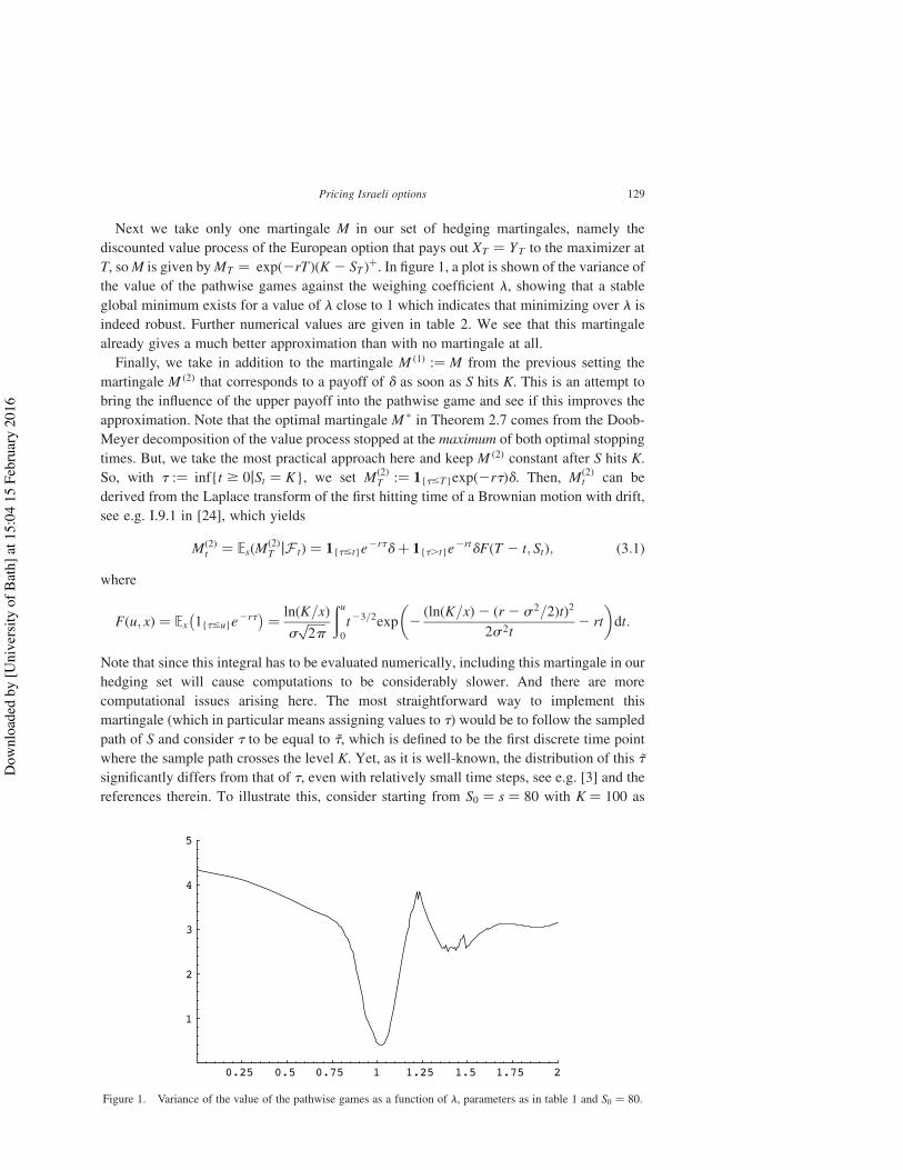
Next we take only one martingale M in our set of hedging martingales, namely the

discounted value process of the European option that pays out XT ¼ YT to the maximizer at

T, soM is given byMT ¼ expð2rTÞðK 2 ST Þþ. In figure 1, a plot is shown of the variance ofthe value of the pathwise games against the weighing coefficient l, showing that a stable

global minimum exists for a value of l close to 1 which indicates that minimizing over l is

indeed robust. Further numerical values are given in table 2. We see that this martingale

already gives a much better approximation than with no martingale at all.

Finally, we take in addition to the martingale M ð1Þ :¼ M from the previous setting the

martingale M ð2Þ that corresponds to a payoff of d as soon as S hits K. This is an attempt to

bring the influence of the upper payoff into the pathwise game and see if this improves the

approximation. Note that the optimal martingale M * in Theorem 2.7 comes from the Doob-

Meyer decomposition of the value process stopped at the maximum of both optimal stopping

times. But, we take the most practical approach here and keep M ð2Þ constant after S hits K.

So, with t :¼ inf{t $ 0jSt ¼ K}, we set Mð2ÞT :¼ 1{t#T}expð2rtÞd. Then, Mð2Þ

t can be

derived from the Laplace transform of the first hitting time of a Brownian motion with drift,

see e.g. I.9.1 in [24], which yields

Mð2Þt ¼ EsðMð2Þ

T jF tÞ ¼ 1{t#t}e2rtdþ 1{t.t}e

2rtdFðT 2 t; StÞ; ð3:1Þ

where

Fðu; xÞ ¼ Ex 1{t#u}e2rt

! "¼ lnðK=xÞ

sffiffiffiffiffiffi2p

pðu

0

t23=2exp 2ðlnðK=xÞ2 ðr 2 s2=2ÞtÞ2

2s2t2 rt

( )dt:

Note that since this integral has to be evaluated numerically, including this martingale in our

hedging set will cause computations to be considerably slower. And there are more

computational issues arising here. The most straightforward way to implement this

martingale (which in particular means assigning values to t) would be to follow the sampled

path of S and consider t to be equal to ~t, which is defined to be the first discrete time point

where the sample path crosses the level K. Yet, as it is well-known, the distribution of this ~tsignificantly differs from that of t, even with relatively small time steps, see e.g. [3] and the

references therein. To illustrate this, consider starting from S0 ¼ s ¼ 80 with K ¼ 100 as

0.25 0.5 0.75 1 1.25 1.5 1.75 2

1

2

3

4

5

Figure 1. Variance of the value of the pathwise games as a function of l, parameters as in table 1 and S0 ¼ 80.


Dow

nloa

ded

by [U

nive

rsity

of B

ath]

at 1

5:04

15

Febr

uary

201

6

hitting level. With the other parameters the same as in table 1 and taking average values after

5 runs of 5000 paths each, we find the empirical probability of the set { ~t # 0:5} to be 0.3720whereas Psðt # 0:5Þ ¼ 0:4182. So the empirical probability is considerably smaller, which

is mainly explained by the fact that there is a significant number of paths of S that actually

do cross K when considered in continuous time but stay below K at each of the discrete time

points.

The problem with this difference between t and ~t is that the process (3.1) is constructedfrom the law of the time-continuous stopping time t whereas later on the sample paths are

generated for a discrete time skeleton corresponding to the stopping time ~t. This causes themapping t 7! EðMð2Þ

t Þ (where E denotes the average over all paths) to be significantly non-

constant. We take a practical approach in solving this by adjusting our way of sampling as

follows. Instead of just sampling from a N ðmD;s2DÞ distributed random variable to

determine the value of the Brownian motion X with volatility s and drift m ¼ r 2 s2=2 at

time point D and translating this into the increase of S on a time interval of length D, we

sample a pair from the joint distribution of X and its running maximum M at time D (or

running minimum when starting from above K). Using this pair we can determine the

increase of S on a time interval of length D together with its running maximum over this time

interval, which in turn allows us to redefine ~t as, say, the middle point of the time interval

under consideration if the running maximum indeed indicates that S has actually crossed K

somewhere on this time interval (and S has not crossed K before). Of course taking the

middle point of the time interval is pretty arbitrary, but the error is at most D=2 ¼ 0:005 andthe exact time at which S hits K only enters, multiplied by 2r ¼ 20:06, linearly. Thus, thisprocedure seems reasonable enough.

The actual sampling from the pair ðXD;MDÞ is pretty straightforward. Making the

substitution Z1 ¼ 2MD 2 XD and Z2 ¼ XD the density function of ðZ1; Z2Þ becomes, cf. e.g.

I.13.10 in [24],

f ðz1; z2Þ ¼ 1{z1$jz2j}expð2m2D=ð2s2ÞÞffiffiffiffiffiffiffiffiffiffiffiffiffiffiffiffiffi

2ps 6D3p z1 exp 2

z212s2D

þ m

s2z2

( ):

Of course the marginal distribution of Z2 is stillN ðmD;s2DÞ and as it is clear from the above

formula, conditional on Z2 ¼ z2 the random variable Z1 follows a Weibull distribution

conditioned on being not less than jz2j. Since we can explicitly calculate the inverse of the

distribution function of this distribution we can sample Z1jZ2 ¼ z2 by standard means.

Now, if we again run the tests from the previous paragraph, we find that with this improved

definition the empirical probability of the set { ~t # 0:5} becomes 0.4152. So the deviation

from the corresponding probability with respect to t has improved from 11 to 0.7%.

Furthermore, on the issue of the processM ð2Þ being a martingale in the discrete time setting,

Table 2. Numerical values with same parameter values as in table 1.

S0

Truevalue



Absolute error/standarddeviation l*

80 20.6 20.8 0.35 0.33 1.0090 12.4 13.2 1.22 0.72 1.40100 5.00 5.00 0.00 – 1.00110 3.64 3.77 0.16 0.33 0.58120 2.54 2.61 0.24 0.14 0.64

C. Kuhn et al.130

Dow

nloa

ded

by [U

nive

rsity

of B

ath]

at 1

5:04

15

Febr

uary

201

6

doing the same tests as above again reveals that on average the difference jEðMð2ÞT Þ2Mð2Þ

0 j iseven closer to 0 than jEðMð1Þ

T Þ2Mð1Þ0 j.

Here are the numerics with the martingales M ð1Þ and M ð2Þ (table 3).

There is some improvement over the values from the previous table. Apparently the

starting point 90 stays an exception as it has a much larger variance and deviation from the

true value than the other ones.

3.2 The convertible bond

A convertible bond is a game contingent claim with payoff processes

Xt ¼ ge2rtSt and Yt ¼ e2rtðK _ gStÞfor t , T and XT ¼ YT ¼ expð2rTÞð1 _ gST Þ, where K . 1 and 0 , g , 1. This game is

called a convertible bond because it can be interpreted as the maximizer having the right to

convert this contract into g stocks, with a guaranteed minimum payment of 1 at t ¼ T. The

minimizer can recall the bond at price K, but then the holder (maximizer) obtains the

opportunity to convert the bond immediately.

The stock price S is now being modelled by a jump-diffusion with non-negative,

exponentially distributed jumps, including dividend payment at rate d with 0 , d , r.

That is, we have that

St ¼ expðsWt þ mt þ JtÞ; ð3:2ÞwhereW is again a Brownian motion and J is a compound Poisson process independent ofW

with jump intensity h . 0 and increments that follow an exponential distribution with

parameter u . 1 (which ensures finite expectations). Note that if we set the drift

m :¼ r 2 d2 s2=2 þ h=ð12 uÞ, then P is an equivalent martingale measure, in the sense

that the process ðexpð2rtÞSt þÐ t0expð2ruÞdSu duÞt$0 is a P-martingale.

Throughout, the optimal exercising strategy of the maximizer is such that he stops as soon

as the stock price exceeds a time-depending level (called exercise boundary, see the doted

line in figure 2). If time to go is very short, the maximizer will exercise right away if

S0 . 1=g but will wait if S0 , 1=g. Also the minimizer exercises once the stock price exeeds

an exercise boundary (see the solid line in figure 2). Coincidence of an exercise boundary

with the upper line which is the level K=g means that there is no “premature” stopping. On

the other hand, St $ K=g implies Xt ¼ Yt and the game is stopped anyway. From figure 2, it

can be seen that never both exercise boundaries lie below K=g at the same time, but it may

happen that there is temporarily no premature exercising. The fact that the minimizer may

recall at stock prices strictly smaller than K=g is caused by the positive jumps in equation

(3.2); see [8] for a discussion of this phenomenon in the perpetual case. A plot of the

corresponding value function can be seen in figure 3.

Table 3. Numerical values with same parameter values as in table 1.

S0

Truevalue



Absolute error/standarddeviation lð1Þ

*lð2Þ*

80 20.6 20.7 0.32 0.17 1.00 20.1090 12.4 11.7 1.20 9.77 1.00 20.70110 3.64 3.72 0.14 0.21 0.58 0.03120 2.54 2.58 0.24 0.08 0.63 0.05


Dow

nloa

ded

by [U

nive

rsity

of B

ath]

at 1

5:04

15

Febr

uary

201

6

Now we turn to the implementation of the pathwise approach. By adding an independent

jump process to the geometric Brownian motion the variance increases and consequently our

sampling variance will also be larger. Tests showed that in our setting doubling the number of

sampled paths from 5000 to 10,000 pretty much makes up for this. In the procedure of

determining the minimizing coefficients with which our martingales are weighted we also

doubled the number of sampled paths, from 300 to 600.

As for the callable put we start out with only the trivial 0 martingale, which results in the

numerics as shown in table 4.

The form of the lower payoff process X for t , T seems to indicate that it makes sense to

try the martingale M ð1Þ defined by Mð1ÞT ¼ g expð2rTÞST . Since ðexpð2ðr 2 dÞtÞStÞt$0 is a

Ps-martingale we have that Mð1Þt ¼ g expð2rt2 dðT 2 tÞÞSt for t , T. With this martingale

the approximation is indeed already significantly better.

Next it seems tomake sense to bring in amartingale that has some connectionwith the upper

payoff Y, therefore we takeM ð2Þ to be the martingale defined byMð2ÞT ¼ expð2rTÞðK _ gST Þ.

0.1 0.2 0.3 0.4 0.5u

1.15

1.25

1.3

1.35

1.4

Figure 2. The optimal exercise boundaries (the dotted line is for the maximizer and the solid line for theminimizer). The u-axes represents time to maturity and the upper line is the level K=g.

00.1

0.2

0.3

0.4

0.5

u

0.5

1

s

1

1.1

1.2

1.3

00.1

0.2

0.3

0.4u

Figure 3. The corresponding value function of a convertible bond, parameters as in table 4. As in figure 2 the plot isobtained by Canadization.

C. Kuhn et al.132

Dow

nloa

ded

by [U

nive

rsity

of B

ath]

at 1

5:04

15

Febr

uary

201

6

We getMð2Þt ¼ expð2rTÞFðT 2 t; gStÞ, where Fðu; xÞ ¼ Ex½K _ Su%, for t , T. Computing F

is now of course more involved than its equivalent in the geometric Brownian motion case.

A closed form formula is still available, but it turns out to be too complex to use it directly in

our simulations in the sense that computing its value takes so long that a simulation of a large

number of paths basically becomes unfeasible. Before addressing this issue we derive the

formula forF, this can be done along the lines of the calculations in [17] e.g. see also this paper

for more details on the functions defined below.

The density of a N ðmu;s2uÞ random variable plus n i.i.d. expðuÞ distributed random

variables is given by

t 7! expðs2u2u=22 ðt2 muÞuÞsffiffiffiffiffiffiffiffiffi2pu

p ðsuffiffiffiu

pÞnHhn21 su

ffiffiffiu

p2

t2 mu

sffiffiffiu

p( )

;

where the Hh functions are given by

HhnðxÞ ¼ð1

x

Hhn21ðyÞ dy ¼1

n!

ð1

x

ðt2 xÞne2t 2=2 dt ð3:3Þ

for n ¼ 0; 1; . . . and Hh21ðxÞ ¼ expð2x2=2Þ.By conditioning on the number of jumps of S up to time u and using that both the Brownian

motion and jump heights in S are independent of this number we can write Fðu; xÞ ¼Ex½K _ Su% as an infinite sum over integrals of y 7! K _ ðx expðyÞÞ against the density above.This yields

Fðu; xÞ ¼ e2luKFlnðK=xÞ2 mu

sffiffiffiu

p( )

þ xe ðs2=2þm2lÞuF

ðmþ s2Þu2 lnðK=xÞsffiffiffiu

p( )

þ expððs2u2=2þ mu2 lÞuÞsffiffiffiffiffiffiffiffiffi2pu

pX

n$1

ðsulu3=2Þnn!

( xIn21 lnðK=xÞ; 12 u;21

sffiffiffiu

p ;2

(suþ m

s

) ffiffiffiu

p( )-

þ KIn21 lnðx=KÞ; u; 1

sffiffiffiu

p ;2

(suþ m

s

) ffiffiffiu

p( ).; ð3:4Þ

with F the cumulative distribution function of a standard normal and the functions In for

n $ 0 defined by

Inðy; a; b; cÞ :¼ð1

y

eatHhnðbt2 cÞ dt:

Table 4. Numerical values with no martingale and parameter values s ¼ 0:4, r ¼ 0:06, K ¼ 1:3, T ¼ 0:5,d ¼ 0:02, g ¼ 0:9, h ¼ 10 and u ¼ 7.

S0

Truevalue



Absolute error/standarddeviation

0.8 1.060 1.031 0.0148 0.241 1.133 1.078 0.0225 0.371.2 1.224 1.139 0.0250 0.541.3 1.272 1.177 0.0231 0.631.4 1.300 1.237 0.0149 0.52


Dow

nloa

ded

by [U

nive

rsity

of B

ath]

at 1

5:04

15

Febr

uary

201

6

By integration-by-parts we can get rid of the integral in this expression and write

Inðy; a; b; cÞ ¼ 2eay

a

Xn

i¼0

b

a

( )n2i

Hhiðby2 cÞ

^b

a

( )nþ1 ffiffiffiffiffiffi2p

p

bexp

ac

bþ a2

2b2

( )F 7by^ c^

a

b

% &;

where the ^ is a þ if b . 0 and a – 0, and a 2 if b , 0 and a , 0; vice versa for the 7.

The first question when implementing these formulas for calculations is where to truncate

the infinite sum involved in the expression of F. Kou suggests that only the first 10–15 terms

are needed in most cases, we took 20 after doing some numerical tests with our parameters.

Furthermore, we see that in order to calculate F for a single pair ðu; xÞ we are required to

compute two double sums in which each summand involves a numerical integration because

of equation (3.3). This is perfectly doable for a just a few evaluations, but as remarked above

it is too involved for our purpose as this involves 50 (namely, the number of time steps)

evaluations of F for a single path and this times 10,000 to perform one simulation of a game.

To overcome this difficulty we did the following. Fix some u . 0 for a moment. The

function f : x 7! Fðu; xÞ is smooth, convex and increasing with f ð0þÞ ¼ K and, on account of

ðexpð2ðr 2 dÞtÞStÞt$0 being a Ps-martingale, such that f ðxÞ2 x expððr 2 dÞuÞ # 0 as x!1.

Furthermore, for h . 0 we have that

f ðxþ hÞ2 f ðxÞ ¼ E1 1{Su[ðK=ðxþhÞ;K=x%} ðxþ hÞSu 2 Kð Þ/ 0

þ hE1 1{Su.K=x}Su/ 0

and since the term in the first expectation stays bounded and tends to 0 when h # 0 it follows

that f 0ðxÞ ¼ E1 1{Su.K=x}Su/ 0

. Given this smooth structure and the fact that 10,000 simulations

would mean 10,000 evaluations of f, it is clear that we can benefit from allowing a small error

in evaluating f (in addition to the error that is already caused by the truncation of the sum and

numerical integration) and taking a number of base points on the x-axis at which f is

approximated by numerically evaluating, after which we interpolate to obtain approximative

values for other x.

More precisely, we simply take linear interpolation and choose a strategy for determining

the base points that allows us to control the maximal error made by interpolating explicitly. In

order to do so, we use that due to the fact that S has only positive jumps, f 0 is bounded belowby the function g given by

gðxÞ :¼ E1 1{~Su.K=x}~Su

h i;

where ~S is the continuous part of S, that is ~St ¼ expðsWt þ mtÞ for t $ 0. Given two base

points xk , xkþ1, the maximal difference on the interval ½xk; xkþ1% between the straight line l

through the points ðxk; f ðxkÞÞ and ðxkþ1; f ðxkþ1ÞÞ and the function f is bounded by the

minimum of f ðxkþ1Þ2 f ðxkÞ and the maximal difference on this interval between l and G,

where G is the antiderivative of g such that GðxkÞ ¼ f ðxkÞ. Note that G qualifies as a usable

bound because we expect it to have a convex structure comparable with f and its maximal

difference with l can be easily computed. Even though this can not be done explicitly, due to

G being convex and smooth and having a representation in terms of F, this maximal

difference can be very quickly and reliably approximated by Mathematica.

The exact implementation looks as follows. We start with an equidistant grid of base points

with typically a grid distance of 0.5 and make sure that our largest base point is chosen such

C. Kuhn et al.134

Dow

nloa

ded

by [U

nive

rsity

of B

ath]

at 1

5:04

15

Febr

uary

201

6

that the difference between f and x 7! x expððr 2 dÞuÞ is smaller than the maximal allowed

error, which we chose to be 1023. After calculating f on these base points we check using the

procedure described in the previous paragraph for each interval between two base points

whether the bound on the error is already smaller than the maximal allowed error. If not, then

we refine the grid by adding the middle point of this interval to it. This we repeat until the grid

is fine enough. Obviously, typically f 0 will be flatter in the regions close to 0 and where x is

large while it is more steep in the region around the point K=g, which translates in the grid

being finer around this point than in both other regions. This operation is feasible on an average

PC although it still takes several hours to complete it for all u [ {0:01; 0:02; . . . ; 0:5}.Having all this established, we can return to our actual goal, namely using the martingale

M ð2Þ in the simulation of the pathwise game. Since the operation for establishing its values

introduces numerical errors to the true value at different stages, one could wonder how much

this influences the martingale property of the sampled process. We checked this by running

10 simulations of 10,000 paths each from the different starting points also used in tables 4

and 5. As before, we look at how much the quantity EðMð2ÞT Þ2Mð2Þ

0 differs from 0 as a

measure for M ð2Þ being a martingale. Note in this perspective also that Mð2ÞT is determined

without using any numerical approximation to F while Mð2Þ0 is deterministic and calculating

its value does make use of the numerical approximation to FðT ; ·Þ. Reassuringly, it turns outthat for all tests and different starting points, jEðMð2Þ

T Þ2Mð2Þ0 j is even smaller than

jEðMð1ÞT Þ2Mð1Þ

0 j. This may seem surprising at first, but it makes more sense if one thinks

about it by looking at Mð1Þt also as a function of the underlying random variable St. This

function has a constant derivative g expð2rt2 dðT 2 tÞÞ, whereas for Mð2Þt this derivative

boils down to g expð2rTÞð›F=›xÞðT 2 t; gStÞ and using the properties of f 0 we discussed

before we see that this function is small for St close to 0 and it is bounded above by

g2expð2rt2 dðT 2 tÞÞ, so in fact this derivative is always smaller. This implies thatMð2Þt has

a smaller variance than Mð1Þt and as the numerical tests indicate, the numerical errors are of

smaller order than this effect.

Now we are ready to move on to the actual simulation of the pathwise game using the

martingale M ð2Þ. The results are as follows (table 6).

We see that this martingale gives a very good approximation, considerably better thanM ð1Þ

did. Some explanation might be found in the fact that the payoff XT of the maximizer at T

looks, due to the face value 1, similar to Mð2ÞT (recall that K ¼ 1:3) while on the other hand,

M ð1Þ and Y look less similar.

Finally, we see whether we can still improve on the values in the previous table by taking

linear combinations of M ð1Þ and M ð2Þ (table 7).

We see there is some improvement here but not too much. Note that the two starting values

with the least good approximations are the ones closest to the level K=g. Furthermore it can

be seen in the plots (and is also indicated by the value 1:300 ¼ K in the tables) that when

Table 5. Numerical values with the same parameters as in table 4.

S0

Truevalue




*

0.8 1.060 1.047 0.0059 0.17 0.34401 1.133 1.113 0.0063 0.25 0.40871.2 1.224 1.199 0.0052 0.35 0.48341.3 1.272 1.241 0.0040 0.49 0.49881.4 1.300 1.279 0.0022 0.45 0.4885


Dow

nloa

ded

by [U

nive

rsity

of B

ath]

at 1

5:04

15

Febr

uary

201

6

starting from S0 ¼ 1:4, the minimizer recalls right away. One could interpret this as an

indication that what is still mainly missing in our set of hedging martingales is a martingale

that is in some sense associated with the payoffs that occur already after short times, when S

quickly enters the early exercise region e.g.

Acknowledgement

We would like to thank an anonymous referee for helpful comments.

References

[1] Bank, P. and El Karoui, N., 2004, A stochastic representation theorem with applications to optimization andobstacle problems, Annals of Probability, 32, 1030–1067.

[2] Brennan, M.J. and Schwartz, E.S., 1977, Convertible bonds: valuation and optimal strategies for call andconversion, Journal of Finance, 32, 1699–1715.

[3] Broadie, M., Glasserman, P. and Kou, S.G., 1999, Connecting discrete and continuous path-dependent options,Finance and Stochastics, 3, 55–82.

[4] Carr, P., 1998, Randomization and the American put, Review of Financial Studies, 11, 597–626.[5] Cvitanic, J. and Karatzas, I., 1996, Backward stochastic differential equations with reflection and Dynkin

games, Annals of Probability, 24, 2024–2056.[6] El Karoui, N., 1981, Les aspects probabilistes du controle stochastique. Ninth Saint Flour Probability Summer

School (Saint Flour 1979), pp. 73–238.[7] Fakeev, A., 1970, Optimal stopping rules for stochastic processes with continuous parameters, Theory of

Probability and its Applications, 15, 324–331.[8] Gapeev, P.V. and Kuhn, C., 2005, Perpetual convertible bonds in jump-diffusion models, Statistics & Decisions,

23, 15–31.[9] Glasserman, P., 2004, Monte Carlo Methods in Financial Engineering (Springer).[10] Ingersoll, J.E., 1977, A contingent-claims valuation of convertible securities, Journal of Financial Economics,

4, 289–322.[11] Ingersoll, J.E., 1977, An examination of corporate call policies on convertible securities, Journal of Finance,

32, 463–478.[12] Jacod, J. and Shiryayev, A.N., 2003, Limit Theorems for Stochastic Processes (Springer), 2.Auflage.[13] Kallsen, J. and Kuhn, C., 2004, Pricing derivatives of American and game type in incomplete markets, Finance

& Stochastics, 8, 261–284.


S0

Truevalue




*

0.8 1.060 1.059 0.0015 0.03 1.44601 1.133 1.131 0.0019 0.05 1.35981.2 1.224 1.219 0.0012 0.14 1.30031.3 1.272 1.263 0.0006 0.37 1.26371.4 1.300 1.294 0.0001 0.60 1.1627


S0

Truevalue




*lð2Þ*

0.8 1.060 1.060 0.0012 – 0.0617 1.27341 1.133 1.132 0.0014 0.03 0.0980 1.12331.2 1.224 1.220 0.0010 0.13 0.0959 1.09911.3 1.272 1.265 0.0006 0.29 0.0299 1.20351.4 1.300 1.294 0.0001 0.60 0.0074 1.1454

C. Kuhn et al.136

Dow

nloa

ded

by [U

nive

rsity

of B

ath]

at 1

5:04

15

Febr

uary

201

6

[14] Kallsen, J. and Kuhn, C., 2005, Convertible bonds: financial derivatives of game type. In: A. Kyprianou, W.Schoutens and P. Wilmott (Eds.) Exotic Option Pricing and Advanced Levy Models, pp. 277–291, (Chichester:Wiley).

[15] Kifer, Y., 2000, Game options, Finance & Stochastics, 4, 443–463.[16] Kolodko, A. and Schoenmakers, J., 2004, Upper bounds for Bermudan style derivatives,Monte Carlo Methods

and Applications, 10, 331–343.[17] Kou, S.G., 2002, A jump-diffusion model for option pricing, Management Science, 48, 1086–1101.[18] Kramkov, D., 1996, Optional decomposition of supermartingales and hedging contingent claims in incomplete

markets, Probability Theory and Related Fields, 105, 459–479.[19] Kuhn, C. and Kyprianou, A.E., 2006, Callable puts as composite exotic options. To appear in Mathematical

Finance.[20] Kyprianou, A.E., 2004, Some calculations for Israeli options, Finance & Stochastics, 8, 73–86.[21] Lepeltier, J. and Maingueneau, M., 1984, Le jeu de Dynkin en theorie generale sans l’hypothese de

Mokobodski, Stochastics, 13, 25–44.[22] McConnell, J.J. and Schwartz, E.S., 1986, LYON taming, Journal of Finance, 41, 561–576.[23] Rogers, L.C.G., 2002, Monte-Carlo valuation of American options, Mathematical Finance, 12, 271–286.[24] Rogers, L.C.G. and Williams, D., 1994, Diffusions, Markov Processes and Martingales Vol. 1, 2nd ed.

(New York: Wiley).[25] Sirbu, M., Pikovsky, I. and Shreve, S., 2004, Perpetual convertible bonds, SIAM Journal on Control and

Optimization, 43, 58–85.


Dow

nloa

ded

by [U

nive

rsity

of B

ath]

at 1

5:04

15

Febr

uary

201

6

pricing israeli options: a pathwise approachak257/kkvs.pdf · pricing israeli options: a pathwise...

Documents