Paths to Success: The Relationship Between Human Developmentand Economic Growth1

by

Michael Boozer2

Gustav Ranis3

and

Frances Stewart4

Preliminary Draft November, 2002Comments Welcome

1We are grateful to Tavneet Suri for outstanding research assistance as well as numerousdiscussions in the development of this project.

2Department of Economics and the Yale Center for International and Area Studies, YaleUniversity. Email: michael.boozer@yale.edu

3Professor of International Economics and the Director of the Center for International andArea Studies, Yale University.

4Professor of Development Economics and the Director of Queen Elizabeth House, Univer-sity of Oxford.

Paths to Success: The Relationship Between Human Developmentand Economic Growth

by

Michael BoozerYale University

Gustav RanisYale University

andFrances StewartOxford University

ABSTRACT

There is growing agreement in the economic development literature thathuman development (HD) is the basic objective of economic activity with eco-nomic growth (EG) as the necessary instrument. However, the precise form ofhow an economy should attain this objective remains imprecise. In this paperwe argue that a large barrier to more precise development policy along theselines requires a more complete description of the inter-linkages between HD andEG. We Þrst show that while the usual view that EG must precede HD hascome up in endogenous growth theoretic models, its empirical importance hasnever been completely documented. Furthermore, the necessity of strong HD asa precursor to sustained growth implies that the uni-directional view of EG ascausal to HD is mis-speciÞed. The principal focus of the paper is in construct-ing an empirical strategy that allows substantial heterogeneity in preference andtechnology parameters across countries. We use country-speciÞc time paths tosummarize the overall �chains� linking EG to HD and HD to EG. We Þnd that,while the use of only one set of these reduced form parameters captures thesample paths of the joint (HD, EG) process rather poorly, the two indices usedin tandem predicts the cross-country sample paths remarkably well.

1 Introduction

The ultimate goal of what is broadly termed �economic development� has long

been recognized to be the overall well-being and utility of a country�s population.

Economists studying development have, however, often focused their studies on

the economic growth of countries. However, this focus implies that it is economic

growth (EG) rather than human development (HD) that is the ultimate goal

of development, perhaps reßecting that EG is viewed as necessary to produce

the Þnal goal of HD. In addition, the choice of how to allocate the proceeds of

EG to HD tends to involve both the preferences of a given country as well as

its current state of development. Such decisions are difficult to render unless a

precise context is speciÞed so that the costs and beneÞts of alternative policies

can be examined.

While observers such as Srinivasan (1994) remind us that there is no inherent

conßict between the dual goals of high HD and high EG, such a conßict persists

in both the academic and policy literature. In our view such a debate seems

to arise and persist largely because the dual relationship between HD and EG

across countries and across time has received far less attention than the deter-

minants of EG across countries. As a result, the debate over the precedence of

HD versus EG and their proper place in development tends to be driven unduly

by the preferences of the debaters and the relative weight of the World Bank�s

WDR and the UN�s HDR. In this paper we take up the task of more carefully

documenting the interrelationship between HD and EG for countries across time

as well as measuring the strength of the dual linkages between them. While the

vast array of resources, preferences, and institutions connecting them remains

something of a �black box�, our research attempts a generalization of the vast

literature focused on EG (the �exogenous� growth literature). In addition, our

work serves as a point of departure for future efforts to understand and explain

the country-speciÞc linkages that determine the strength of the links from EG

2

to HD and vice versa.

Our research is inspired by the inductive evidence presented in the earlier

work of Ranis, Stewart, and Ramirez (2000) (hereafter RSR) who examined

country-speciÞc paths in HD and EG measures over the period 1960 to 1992.

While their work only began to address the causal factors of HD and EG across

countries, their evidence makes for a compelling case that the time paths of HD

and EG for a given country are not independent of each other. In particular,

their evidence damages the traditional view of EG as predetermined relative to

HD. They found that, while short run gains in EG may be gained independent

of HD levels, such gains in EG appear to be short-lived unless HD levels are

also upgraded prior to, or in tandem with, EG-centric policies. This Þnding

alone means that the traditional approach of modeling EG as predetermined

is mis-speciÞed and that HD levels play an important �feedback� role in the

determination of subsequent growth. Thus even a social planner (or a policy

maker in a decentralized economy) with EG-centric preferences would be remiss

to ignore the role of HD upgrading on the sustainability of growth. This evidence

implies that the debate over HD and EG outcomes as an �either / or� debate is

misplaced, but that research and data collection efforts should focus on modeling

this joint process, and on the production of HD as an endogenously determined

input into the production of future EG, just as EG is required for the production

of HD. The use of the currently favored �one way� path models are likely to lead

to the adoption of policies focused excessively on EG, policies which may yield

only transitory gains in EG (what RSR refer to as �EG lopsided� outcomes) and

steady-states which are unaltered in the long run.

The empirical strategy we develop in this paper is driven by the observa-

tion that the individual processes linking EG to HD and HD to EG are by no

means homogeneous across countries. While assuming a common production

function across countries was common in the early cross-country growth litera-

ture, most researchers now have serious misgivings about such assumptions and

3

their approach.5 Instead, we allow for country-speciÞc strengths of the �chains�

linking EG to HD (Chain A) and HD to EG (Chain B). These chains are simply

a description of factors that encompass the relationship between HD and EG

in both directions, as shown in Figure 1. We rely heavily on the time series

dimension of our data to identify such country-speciÞc measures. We then pool

this collection of the 196 reduced form parameters measuring the strength of the

two chains for each of 98 countries to learn about the joint process of the two

HD and EG chains. Our measure of the Chain B strength is a generalization

of the �exogenous� technological change variables that drive sustained growth

in the neoclassical model. We Þnd that levels of HD drive subsequent growth,

a Þnding that was illustrated in the evidence of RSR, and is replicated in our

framework. In other words, we allow human capital to be a causal factor of

sustained growth, which may itself be endogenously produced.

In agreement with the earlier literature, we Þnd that EG is an important,

indeed an indispensable, input into the production of HD (Chain A). Far less

research attention has been paid to date to this less conventional production

function, the HD improvement function (HDIF), and thus our approach here is

comparatively ad hoc. Our strategy for dealing with the HDIF differs in two

important respects from our Chain B approach, for both data and conceptual

reasons. On the data front, we tend to have less time series coverage on our

measures of HD than for EG and can therefore really only examine HD changes

over the latter half of our sample period. The conceptual difference stems from

our prior that the building of HD infrastructure and the realization of its beneÞts

(e.g. life expectancy) occurs with a longer and more uncertain lag than in

improving EG, which is the Chain B outcome. We therefore use the country-

speciÞc relationship between predetermined �early� EG and �late� improvements

in HD as our measure of the strength of Chain A.

5See Solow (2000) and Srinivasan (1995) for critiques, and Durlauf and Quah (1999) for

an overview on approaches that abandon the strong form of this homogeneity.

4

While our empirical strategy for estimating the strength of Chain A is not

quite as �assumption free� as the strategy for Chain B, both rely on the time

series dimension of the data to estimate country-speciÞc summaries of the re-

lationships between HD and EG. We therefore differ from the standard �cross-

country regressions� literature that places strong homogeneity restrictions on

preference and technology processes across countries. Not using purely cross-

sectional data on HD and EG implies that there are no �simultaneous equations�

in our framework. However, we do Þnd that the joint sets of parameters across

countries measuring the Chain A and Chain B linkages are essential for describ-

ing their joint time series paths. For example, were it the case that EG were

�instrumental� or predetermined for HD, while HD does not Granger cause EG,

then the Chain B index would be sufficient to predict the performance of coun-

tries along the EG dimension. However, our empirical evidence indicates that

it is essential to use the simultaneous strengths in the Chain A and Chain B

linkages to predict the observed time series paths of these variables from 1960

to 2000. While it is true that many countries tend to score well or poorly on

both of these measures if they score well or poorly on one of them, many other

countries fail to reach the virtuous (and self-reinforcing) plateau of high EG and

high HD. Countries with weak Chain A links but strong Chain B links tend to

end up in the EG-lopsided state, with high EG but poor HD. This Þnding was

foreshadowed by the RSR Þndings and it represents the strongest evidence in

our paper against the view that the univariate process in EG is sufficient to

describe the joint EG-HD process. In fact, even if we are interested in under-

standing only EG as an outcome, our evidence shows that the dual Chain A

and Chain B measures are required. As per RSR, upgrades in HD via strong

links in Chain A are a necessary precondition to sustained (i.e. non-decreasing)

growth.

The rest of the paper is organized as follows. In Section 2, we update the

RSR Þndings and then review some of the previous literature on the HD-EG

5

relationship. Section 3 discusses our measurement framework for the strength

of the links in Chain B, as well as generalizing it to encompass the neoclas-

sical growth model as a special case. In Section 4 we discuss the analogous

measurement framework for measuring the links in Chain A. In Section 5 we

consider the two measurement devices in tandem and discuss their successes and

shortcomings. Here we show how planning or decentralized policy making in an

environment that ignores the role of HD in producing sustained EG can lead to

EG-lopsided outcomes and failure to accomplish the long-run enhancement of

development. Section 6 concludes.

2 Summary and Update of Previous Findings

and Literature

The previous literature on HD, EG, and their inter-relationships is too vast to

summarize here. Instead, we start by Þrst updating the prior work by RSR

on the two-way HD-EG relationship and, subsequently, referring only to the

literature that relates directly to our paper.6

Prior work by RSR examined the inter-relationships between HD and EG

for a large sample of developing countries for the period from 1960 to 1992. We

now review the most important implications of this paper for our work, and

update their results to 2000. RSR focused on documenting the two chains that,

when mutually reinforcing, lead to higher growth and higher human develop-

ment outcomes. These two Chains are illustrated in Figure 1 where we can see

that the strength of the links in say Chain A can be hypothesized to depend

on a number of factors, including, with respect to households, such factors as

income distribution, poverty rates, the level of female control over income, and,

with respect to governments, total expenditure, social expenditure and priority

6See Ranis, Stewart and Ramirez (2000) and Ranis and Stewart (2000).

6

ratios, plus factors that determine the efficiency of the human development im-

provement function. The reverse ßow, Chain B, i.e. from HD back to EG, nests

the more conventional production function, with the speciÞc prediction that HD

affects the trend or sustained component of growth, what we later refer to as

the growth trajectory. While economic growth provides the resources to permit

improvements in human development, human development is not only the Þnal

objective of an economy but also an input to additional increments in economic

growth. RSR identify the mutually reinforcing state of high EG-high HD as a

virtuous cycle and the opposing mutually depressing state as a vicious cycle.

Two asymmetric alternatives are also possible, as outlined below.

INSERT FIGURE 1

This initial work made an effort to econometrically examine the signiÞcance

of the various variables affecting both Chain A, from growth to human devel-

opment, and Chain B, from human development to growth. RSR found that,

for Chain A, GDP per capita growth, the social expenditure ratio and female

school enrollment rates all had a signiÞcant effect on HD. Similarly, in the case

of Chain B, the initial level of human development, as well as its change, the

investment rate, and the distribution of income all had a signiÞcant effect on

EG.

In the same analysis, they proposed that countries are likely to fall into

four possible categories when their EG-HD performance is compared to the

average developing country performance. Countries that exhibit above average

improvement in both human development and in growth fall into the virtuous

cycle, whereby strong links in both Chains A and B are mutually reinforcing.

On the other hand, the vicious cycle describes countries with relatively poor

performance on both growth and human development, with strong Chain A and

B linkages reinforcing each other over time. Finally, there are two possible cases

of lopsided performance, with some countries having better than average growth

but worse than average human development improvement, while others do worse

7

on growth and better than average on the human development dimension. Over

time, such lopsided development is not likely to persist since eventually the

weakly performing dimension will act as a brake on the other, leading to the

vicious cycle case, or, if linkages are strengthened over time, possibly through

policy change, a virtuous cycle.

Following RSR, Figure 2 shows the country classiÞcations, by region, in HD

and EG performance over the period 1960 to 2000. We use the infant mortality

shortfall reduction (IMSR) as the measure of HD change. It is standard in the

human development literature to measure changes in infant mortality, life ex-

pectancy, or adult literacy, as a shortfall (or gap) reduction. This helps account

for �ceiling (or ßoor) effects� for countries which near the theoretical boundaries

of, for example, 3 percent for infant mortality and 85 years of age for life ex-

pectancy. As countries near those boundaries, their actual change in the HD

measure may be small. However, using the fraction of the remaining shortfall

from the theoretical limit can account for this boundary effect, by accounting

for the size of the shortfall.7 As the measure of EG, we use the annual growth

rate in real per capita GDP. Figure 2 shows the relative HD-EG performance

of our sample of developing countries, by region, not including the Eastern Eu-

ropean countries. The averages that are used to deÞne the virtuous, vicious,

EG-lopsided and HD-lopsided cycles are population weighted developing world

averages (again excluding Eastern Europe). We should note, not surprisingly,

the dominance of East Asian countries in the virtuous cycle quadrant and that

of Sub-Saharan Africa in the vicious cycle quadrant.

INSERT FIGURE 2

RSR also argue that the path taken by an economy over time is extremely

important. It appears that only via the HD-lopsided cycle can a country in

7For example, if the underlying process is logistic, the shortfall reduction comes close to

converting the logistic path into one of nearly constant slope. This is the property we seek if

the goal is to abstract from ceiling or ßoor effects, where the slope of the logistic curve goes

to zero as it approaches its upper and lower limits.

8

the vicious cycle transit to the virtuous cycle. If a country attempts to transit

to the virtuous cycle via EG-lopsidedness its growth improvements will tend

to be short-lived and it returns to the vicious cycle. The main implication of

this is that a country Þrst needs to improve its HD before growth can become

sustained. While Figure 2 gave us a broad picture of the performance over forty

years, we can break this down into a decade-by-decade analysis to study the

transition of each of these countries (see Table 1 for the decades 1960-1970, 1970-

1980, 1980-1990 and 1990-2000). Once again, the decomposition into virtuous,

vicious, HD-lopsided and EG-lopsided cycles is based on population weighted

averages. Figure 3 illustrates these same transitions by region. In this two-

dimensional representation, the paths to �success� for the countries that made it

to the virtuous quadrant of high EG and high HD were non-linear. The number

of countries that made that transition from low EG to sustained high EG was

small. But the number of countries which tried the one-dimensional approach

to reaching high EG - i.e. by not simultaneously upgrading their HD - were

many, and without exception, their gains in higher EG were not sustained.

INSERT TABLE 1

INSERT FIGURE 3

To try and understand more about the roles played by underlying variables

in Chains A and B, RSR performed some regression analysis. We replicate

these here, once again updating our data set to the year 2000. Tables 2 and 3

report the results of these regressions. For Chain A, we use the infant mortality

shortfall reduction 1960 to 2000 as the measure of HD improvement. As Table 2

illustrates, growth in GDP per capita over the early parts of the sample period,

1960-1970, is highly signiÞcant in determining HD performance. Moreover, the

gross primary enrollment rate as well as the gross female primary enrollment

rate, public expenditure ratios on education and health are all signiÞcant. Table

3 shows the results for Chain B. Both HD measures, i.e. life expectancy and

the literacy rate, have signiÞcant effects on growth, as does the gross domestic

9

investment rate.

INSERT TABLE 2

INSERT TABLE 3

This completes the replication exercise from RSR. The most important im-

plications of their work are evident. It seems countries need to update their HD

prior to EG in order to beneÞt from sustained growth. We nowmove on to a brief

general literature review. Starting with Srinivasan (1994), his critique makes

clear that, while EG provides the instrumental means by which HD capacities

are improved, EG has historically not always been viewed as the sole objective of

development. Srinivasan does, however, clearly adopt the separability between

the EG and HD processes as portrayed in a standard budget line-indifference

curve analysis when arguing against using an HD index as the sole standard by

which development should be judged. While the notion that an index of HD,

necessarily more arbitrary, should usurp EG as the ultimate measure of suc-

cessful development is fraught with many measurement and conceptual issues,

our empirical evidence contradicts the conventional view that the development

process is one solely from EG to HD. Of course, if all countries tend to spend the

proceeds of growth on HD in much the same way, then EG can serve as a simple

summary statistic for the bivariate process. Aturupane, Glewwe, and Isenman

(1994) analyze this question empirically and Þnd that a single index based on

EG accounts for only about one-third of the variation in HD improvements.

Thus, even with the traditional view, that EG and HD form a one-directional

path from means to ends, clearly how policies and infrastructures are developed

matter for the ultimate increase in HD.

It is not hard to see why EG has retained its place as the focus, if not

the ultimate goal, of development economics for so long. EG is more easily

measurable and has the virtue that it has a tight theoretical basis (e.g. Solow

(1956) and much of the literature which followed). However, the neo-classical

growth model did not completely eliminate the ad hoc nature of the empirical

10

speciÞcation efforts, as the large volume of cross-country growth regressions

published from the late 1980�s until the present illustrates. The sensitivity

analysis performed by Levine and Renelt (1992) represents one early attempt

to plow through the various empirical speciÞcations suggested. In a related

strain of the literature, work by Durlauf and Johnson (1995) raised issue with

the stringent homogeneity assumptions implied by a strict interpretation of the

Solow model. They stress that countries should only be pooled across �clubs�,

which share a common form of steady-state income, and should not be all placed

into a common cross-country regression.8

Meanwhile, the recent endogenous growth literature, primarily theoretical,

along the lines of Romer (1986) and Lucas (1988) has further muddied the

precision of the neoclassical growth model for the empirical speciÞcation of

growth. In our empirical speciÞcation for EG and the Chain B links, we start

with the speciÞc aspects of EG we wish to measure, and then show how our

framework Þts in with the general characteristics of the neoclassical growth

model. In so doing we want to capture the relevant lessons from both the

heterogeneity (observed and unobserved) and the endogenous growth literature

in starting with a ßexible measurement framework.

The literature on HD and Chain A is by comparison much less voluminous.

Indeed, uncertainty along many dimensions of Chain A pervades the develop-

ment of a suitable measurement framework to measure the human development

improvement function. There are, of course, a considerable number of microeco-

nomic studies that illustrate the importance of various inputs, such as education,

health, potable water, as well as of such variables as the proportion of income

earned by women in the household, but a full analysis of the HDIF is still want-

ing (see Strauss and Thomas (1995)). We do not dwell on this intricate problem

in the context of this paper, but instead try to characterize the heterogeneity

8Indeed, Solow (2000) himself provides a critique of the empirical convergence literature

as well as of applying a homogeneous production function setup to explain growth across

countries.

11

in HDIF �efficiency� across countries as our summary measure of Chain A.

3 Income Paths: Measuring the Strength of the

Links in Chain B

We begin the discussion of our measurement framework for the two chains with

a focus on Chain B. This is because of the longer time series data available for

each country on EG as well as because of the more advanced state of knowl-

edge on that production function. The framework permits us to use the time

series dimension of the data to construct a country-speciÞc summary measure

of the strength of the underlying linkages in Chain B. In addition, it highlights

how ßexible we can make the cross-country variation in the parameters and

thus avoid the stringent homogeneity assumptions of the cross-country growth

literature. We can then relate our measurement framework to the standard

Solow-type neoclassical model and use this to modify our framework so as to

not �penalize� the high average growth countries. Our resulting strategy is then

easily interpretable in a Solow context, albeit one in which the usual cross-

country homogeneity assumptions are discarded and one in which the driving

force behind sustained growth becomes an empirical question.

As discussed above, one of the more intriguing, and testable, implications

of the RSR analysis is that countries that did not upgrade their HD levels in

tandem or prior to their attempts at higher EG tended to Þnd their gains in EG

short-lived. This non-linear relationship is elegantly re-displayed for our data

in Figure 3, which traces out the paths relating HD and EG over the 1960 to

2000 sample period.

Incorporating the information in a time series path of each country in the

(HD − EG) plane for a more statistical, and less qualitative, analysis is quitedifficult. Approaching the problem directly, each country has its own unique

12

non-linear path that it follows during our sample period 1960 to 2000, and such

unique non-linearity makes for a difficult measurement problem. Our solution

is to break the bivariate path in (HD−EG) into the univariate path for EG fora given country over time, which we label the growth trajectory. This provides

us with a univariate measure of the �sustainability� of the EG path, and we can

then see to what extent HD levels affect this EG trajectory. We emphasize from

the outset that neither the concept nor our measure of sustainability should be

equated to higher average growth. Both low growth and high growth countries

can score well on sustainability. But a country which experiences only a few

periods of higher EG, followed by a lapse to a lower growth state may have high

average EG over our sample period, but still score lower on our sustainability

measure. We should also note that our measure of sustainability, referred to

as the growth trajectory, is far more general than the usual notion of sustained

growth as it includes countries that may even have negative average EG over

the period, but are on a positive EG trajectory.

To measure these paths, we propose a simpliÞed approach that extracts the

linear time path of EG. If growth is constant or rising, the slope of this time

path will be zero or positive. We want transitory increases in EG not to be

counted as a positive growth trajectory. To accomplish this, we use a simple

decomposition from panel and hierarchical data methods that breaks down the

sample path of growth rates git for country i over the period 1960 to 2000 into

a country-speciÞc mean, a country-speciÞc trend, and idiosyncratic ßuctuations

around both of these parameters as follows:

git = αi + βit+ uit (1)

Note that these are a set of country speciÞc regressions yielding a collection

of estimated �αi and �βi Þtted values for each country. Then, in a second-stage

regression, we try to explain the country-speciÞc slope parameters that cap-

ture the growth trajectory, �βi with our regressors of interest, here mainly HD

13

measures.9

Note that if growth is simply random ßuctuations around a constant mean

rate, the estimated trend would be zero and the ßuctuations would be absorbed

into the error terms uit. Non-sustained jumps in growth will tend to raise the

estimated αi for a country, but also associate it with a negative βi. Empiri-

cally, there is a slight negative trend in growth rates for our entire sample of

countries over this time period, although we can treat �βi = 0 as our baseline,

with countries with zero or positive �βi�s being characterized as having a positive

EG trajectory and countries with �βi < 0 as having non-sustained or declining

growth. Our eyeball examination of the 86 country-speciÞc regression Þts indi-

cate that this HLM decomposition of growth rates provides a good measure of

sustainability.

It is also useful to compare the relationship of our HLM procedure to the

treatment of the time-series information in growth rates used in the literature

on convergence (e.g. Barro and Sala-i-Martin (1992)). Many researchers in this

literature �average out� the time dimension in their samples, and focus on average

growth rates over the sample period. Note that this information is contained

in our HLM measures as well, as each country-speciÞc OLS regression Þts the

mean. Thus, (using the over-bar to denote the time-averaged sample mean):

gi = �αi + �βiT + 1

2(2)

since the mean of the time trend t in a sample of length T is T+12 . Thus, by

suitably combining the information in the HLM effects of �αi and �βi, we could

simply reproduce the information typically used in cross-country growth regres-

sions. However, the HLM factorization allows us to separate out the direction

9This procedure falls under the class of �Hierarchical Linear Models� or HLM as advanced

by Bryk and Raudenbusch (1992) in the Þeld of psychometrics. See Boozer and Maloney

(2001) for the relation of HLM to econometric methods more familiar in economics, as well as

an application of the method for studying growth in individual-speciÞc test score trajectories

by age.

14

of the growth trajectory, which we deÞne to be sustainability, from the average

level of growth. Thus, a country which has a constant level of growth, be it low

or high, would score a 0 on a measure of sustainability by this deÞnition. Figure

4 shows the relationship between our measure of sustainability ( �βi) and the av-

erage growth rate for each country. Countries such as Korea and Singapore have

high growth rates from 1960 to 2000, but score only average on this measure of

sustainability. In fact, this �pure� or mechanical HLM approach tends to actu-

ally penalize countries with high average growth rates as far as the sustainability

measure goes. To see this, note the empirical plot of the Þtted HLM coefficients

of �βi versus �αi in Figure 5. There is a strong negative relationship between the

two estimates across countries, indicating that countries with higher average

growth rates will tend to score poorer on our proposed sustainability measure

of �βi.

INSERT FIGURE 4

INSERT FIGURE 5

While we experimented with a few ad hocmodiÞcations to our HLM-inspired

measurement approach, we returned to the cross-country growth literature to

incorporate an important omitted factor that plays a role in determining the

time-series movements in cross-country growth rates.10 Our goal is to revise

our initial measure of sustainability in EG so as to not �mechanically� penalize

high-growth countries, as the pure HLM approach does. We devote the next

sub-section to relating our statistical HLM framework to the neoclassical growth

literature, and then propose a simple modiÞcation to our HLM procedure that

does not suffer from these mechanical difficulties.

10One approach was to ask, for a given �αi, which countries had a higher �βi? Here, countries

like Singapore and Korea, which had only middling values of �βi, due in part to their high

average growth levels, had the highest values of the �residual beta� measure, after factoring

out their high �αi values. The approach that we describe below has the same ßavor as this

approach, but is less ad hoc and ties in closely with the neoclassical growth literature.

15

3.1 The Relationship of Our Measurement Framework to

the Neoclassical Model of Growth

The last 15 years have seen a resurgence in research on both the theoretical and

empirical causes of economic growth across a broad spectrum of countries. It

is a fair summary of both the theoretical and empirical literature to say that

it has focused in particular on how the cluster of �developed� countries is able

to sustain growth, absent some force creating technological advances offsetting

the declining marginal product of physical capital for a given country. Both

strands of the research literature have focused intently on the technological

progress explanation for differences in growth rates because it has important

implications for how we revise the neoclassical growth model of Solow to allow

for the possibility that the growth rates of clusters of countries actually diverge

over the long run.

The empirical work that led to the renewed interest in the sources of growth

focused on the trends in long run growth in the industrialized and nearly indus-

trialized countries. Authors such as Baumol (1986) tended to Þnd that growth

rates converged in accord with the simpliÞed neoclassical model within �clubs�

of countries, but diverged across such clusters of countries in the long run. This

provided the impetus to try to document or refute this Þnding in a broader set

of countries, as well as provide an explanation for how this could occur in a

well-speciÞed economic model, as in Romer (1986). What appears to have been

left out of this renewed focus over the past 15 years, however, is that growth

trajectories may well have a �life-cycle� aspect to them, in that factors that mat-

ter early in the growth path for a given country may matter far less later in the

life-cycle of that country. Indeed, the earlier literature on the factors affecting

economic growth often had some threshold that constituted a �take-off� point,

beyond which economic growth increased more rapidly. Kuznets, Lewis, and

Rostow were among the authors who provided possible, if differing, explana-

tions for why the life-cycle of economic growth was not purely constant. These

16

authors were writing at a time when some countries were making the transition

from low growth to high (sustained) growth before their very eyes, and so they

were motivated to try to explain why some countries were able to attain this

higher plateau, while other economies appeared to remain stagnant.

The data sources that were available to researchers in the 1980�s offered a

portrait of a broad cross-section of both developed and developing countries

on a number of indicators. From 1960 to the present, only a few countries in

the developing world have made the transition from a low growth state to a

sustained high growth state. Thus, this time window does not permit so much

a view into what allows this transition to be made as it allows us to examine

the far more numerous examples of where attempts at high growth policies

have failed to produce sustained success. When we look at the differences in the

growth rates over this period, it is not at all clear whether the �new growth�

literature and its focus on �technological change� can explain why, for example,

Botswana enjoyed greater success than other countries in Africa. We argue

that with a suitably evolutionary notion of what is meant by �labor augmenting

technical change� we can place both developing and more developed countries

on a uniÞed life-cycle growth path. We wish to establish a bridge between the

recent endogenous growth literature which focuses on the production of ideas

and the role of technological diffusion and the earlier literature which focused

on earlier stages in the growth transition of countries and considered elements of

progress beyond that narrow focus. Uzawa (1965) represents a critical �missing

link� in this regard in that he presents a two-sector endogenous growth model

in which the �health and education� sector constitutes the reproducible input

responsible for endogenous growth.

When we look at the conventional production function approach, we usually

focus on growth rather than on income per capita or levels of output. While

authors such as Barro (1997) and Quah (1996) have noted that the time-series

movements in per-capita output are a trivial fraction of the cross-country vari-

17

ation in levels of output per capita, our focus here is more on describing the

trajectories of growth that we observe during our sample period, as the levels

are too much a function of initial conditions and a myriad of political and cul-

tural factors. This combination of factors makes the attempt to explain the

cross-country patterns of output levels a precarious venture at best. Instead, we

ask what factors lead to sustained growth over the 1960 to 2000 period covered

by our sample, as well as the contra-positive to this question, which is why do

some countries fail to sustain attempts to reach a high level of growth. We focus

in the next section on a framework for measuring what is meant by �sustained�

growth. As we will see, our measurement framework needs to confront the em-

pirical fact that there is a strong propensity for growth rates to converge, as

opposed to income levels that are the focus of the convergence literature.

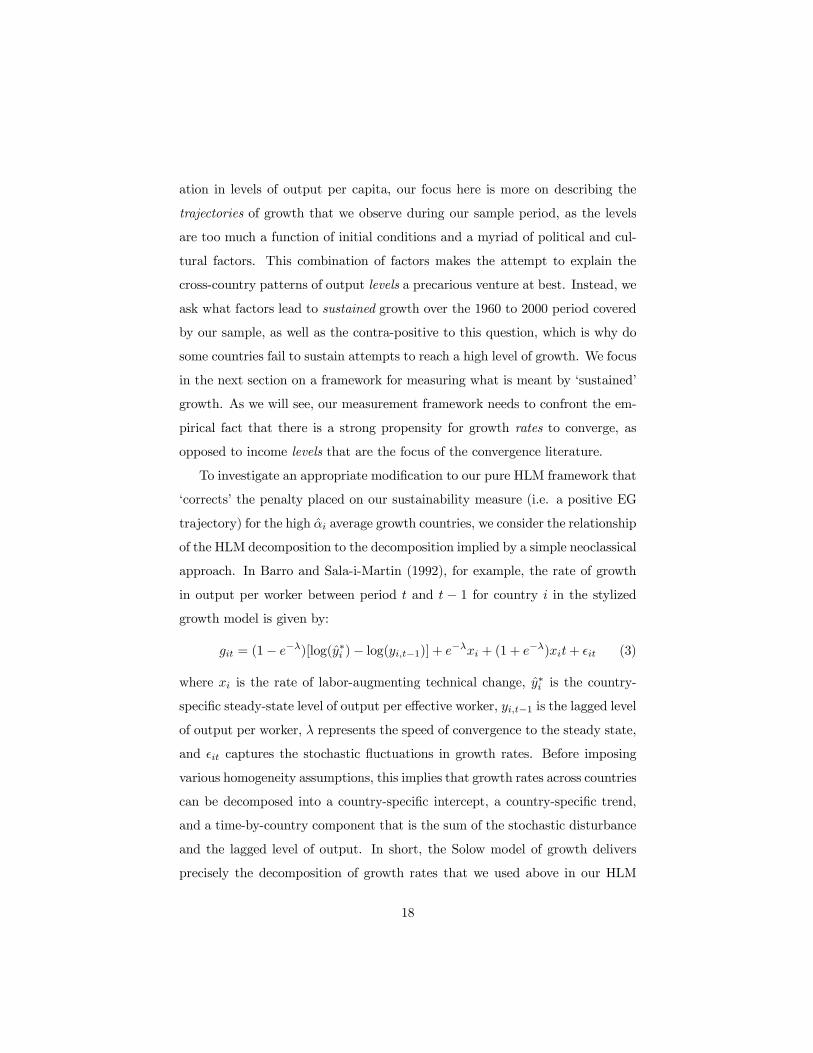
To investigate an appropriate modiÞcation to our pure HLM framework that

�corrects� the penalty placed on our sustainability measure (i.e. a positive EG

trajectory) for the high �αi average growth countries, we consider the relationship

of the HLM decomposition to the decomposition implied by a simple neoclassical

approach. In Barro and Sala-i-Martin (1992), for example, the rate of growth

in output per worker between period t and t − 1 for country i in the stylizedgrowth model is given by:

git = (1− e−λ)[log(�y∗i )− log(yi,t−1)] + e−λxi + (1+ e−λ)xit+ ²it (3)

where xi is the rate of labor-augmenting technical change, �y∗i is the country-

speciÞc steady-state level of output per effective worker, yi,t−1 is the lagged level

of output per worker, λ represents the speed of convergence to the steady state,

and ²it captures the stochastic ßuctuations in growth rates. Before imposing

various homogeneity assumptions, this implies that growth rates across countries

can be decomposed into a country-speciÞc intercept, a country-speciÞc trend,

and a time-by-country component that is the sum of the stochastic disturbance

and the lagged level of output. In short, the Solow model of growth delivers

precisely the decomposition of growth rates that we used above in our HLM

18

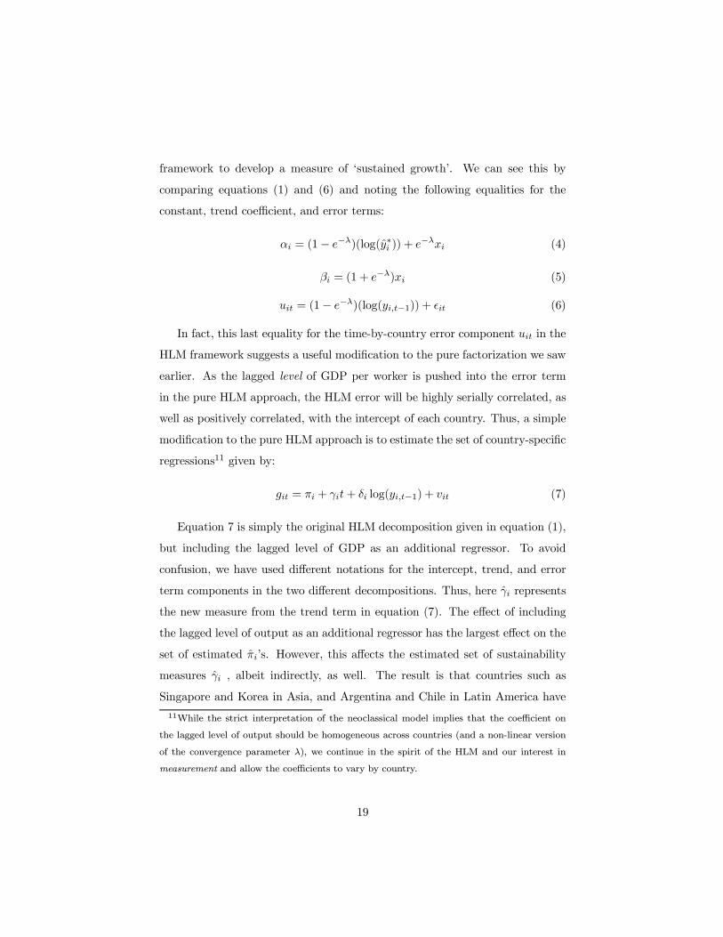
framework to develop a measure of �sustained growth�. We can see this by

comparing equations (1) and (6) and noting the following equalities for the

constant, trend coefficient, and error terms:

αi = (1− e−λ)(log(�y∗i )) + e−λxi (4)

βi = (1+ e−λ)xi (5)

uit = (1− e−λ)(log(yi,t−1)) + ²it (6)

In fact, this last equality for the time-by-country error component uit in the

HLM framework suggests a useful modiÞcation to the pure factorization we saw

earlier. As the lagged level of GDP per worker is pushed into the error term

in the pure HLM approach, the HLM error will be highly serially correlated, as

well as positively correlated, with the intercept of each country. Thus, a simple

modiÞcation to the pure HLM approach is to estimate the set of country-speciÞc

regressions11 given by:

git = πi + γit+ δi log(yi,t−1) + vit (7)

Equation 7 is simply the original HLM decomposition given in equation (1),

but including the lagged level of GDP as an additional regressor. To avoid

confusion, we have used different notations for the intercept, trend, and error

term components in the two different decompositions. Thus, here �γi represents

the new measure from the trend term in equation (7). The effect of including

the lagged level of output as an additional regressor has the largest effect on the

set of estimated �πi�s. However, this affects the estimated set of sustainability

measures �γi , albeit indirectly, as well. The result is that countries such as

Singapore and Korea in Asia, and Argentina and Chile in Latin America have

11While the strict interpretation of the neoclassical model implies that the coefficient on

the lagged level of output should be homogeneous across countries (and a non-linear version

of the convergence parameter λ), we continue in the spirit of the HLM and our interest in

measurement and allow the coefficients to vary by country.

19

much higher sustainability measures when we use the modiÞed framework than

under the pure HLM framework that tended to penalize them for their high

average growth rates and levels of output.

Figure 6 presents the relationship between this new measure of sustainability

(�γi) and average growth rates. It is clear from this Figure that, whereas the

original HLM measure of sustainability was slightly negatively correlated with

average growth, as in Figure 4, Figure 6 shows the modiÞed measure to be

mildly positively correlated with average growth. Contrasting Figures 4 and

6, it is thus clear that, by using the modiÞed HLM procedure, countries like

Korea, Singapore, and Thailand are no longer penalized for their high growth.

Likewise, countries such as Haiti, Bangladesh, and Cambodia are corrected

downward under the modiÞed procedure, and so do not score nearly so well

on sustainability as under the original HLM framework. Figure 7 plots the

original (�βi) versus the modiÞed (�γi) sustainability measure. While the two

measures are certainly positively correlated, it is clear that the correlation is by

no means perfect. As the modiÞed procedure has fewer measurement problems

and correctly captures the trend, level, and lagged output components of growth

implied by the standard Solow model, we utilize only the modiÞed sustainability

measure, �γi, in what follows.

INSERT FIGURE 6

INSERT FIGURE 7

The mapping between this modiÞed HLM approach and the stylized neoclas-

sical model has another appeal. Notice that expressions for the intercept and

trend effects of αi and βi hold, respectively, for πi and γi as well. The striking

implication from the underlying model for the trend effect δi versus the intercept

effect πi is that only sources of productivity enhancements for labor (denoted

as xi in the model above) should affect δi, whereas both xi as well as vari-

ables which help explain the steady state level of output per worker should help

describe the variations in the intercepts across countries. Put differently, the

20

neoclassical model implies the important exclusion restriction that only factors

which improve labor productivity should be associated with our sustainability

measure, whereas factors which affect both steady-state levels as well as vari-

ations in labor productivity should explain the cross-country variations in the

intercepts.

The modiÞed HLM approach also removes one of the common criticisms of

cross-country growth regressions, in that they have a �kitchen sink� type ßavor

to them. It is common in cross-country regression studies for the researcher

to simply pool the cross-section and time series dimensions of the data and

treat it all as �one kind� of variation. The modiÞed HLM framework instead

relies exclusively on the time-series path of the data in the Þrst stage, breaking

it into a linearized version. However, this decomposition meshes entirely with

the stylized Solow model, a theory that delivers a very precise way on which

variables should affect growth. Thus, if we take a variable such as the investment

rate, which is well known to correlate with pooled growth rates in a standard

cross-country growth regression, the Solow model predicts that it should not

correlate with the estimated trend component within the HLM framework (see

equation (5)). Only variables which are the empirical counterpart of xi, which

is technical progress in the traditional view, should affect the trend component

of growth. The modiÞed HLM framework allows us to be more broad-minded

than the pure neoclassical model and ask the empirical question of what affects

sustained growth. This exercise gains credibility because when the modiÞed

HLM framework is viewed via the stylized neoclassical model, variables such

as the investment rate should help explain only the intercept (via its effect on

steady-state output) and not the trend.

21

3.2 What Explains Sustained Growth in Developing Coun-

tries?

Now that we have a summary measure of the country-speciÞc time series of

growth paths via the modiÞed HLM framework, �γi, we can test the hypothe-

sis of RSR that attempts to increase EG without a prior or contemporaneous

strengthening of HD levels implies that such gains will be short-lived. We can

also ask, more generally, what explains sustainability in EG for our sample of

developing countries. Largely for comparison purposes, we also examine the

impacts of our variables on the average growth rate levels given by �πi, where

the distinction in what variables should determine �πi is less clear.

Having summarized the time series growth path by a single scalar, the speci-

Þcation question now is how to treat the time-series vector for each explanatory

variable. We follow the usual practice in HLM-based models and use the time

average of the explanatory factors, after Þnding that this appeared to be a good

summary of the underlying period-by-period regressions. The second issue of

speciÞcation is whether we want to use HD levels or HD growth rates. We work

with levels because we feel they are more tightly associated with labor produc-

tivity. In addition, large HD upgrades may still leave a country with poor HD

levels and vice versa, and so it is not clear that HD changes are the appropriate

concept. In the language of RSR, the index that determines the non-linear point

of �takeoff� in the EG process is determined by the level of HD, and not purely

its rate of growth.12

Thus we specify an empirical model relating sustainability in EG to HD as

12In this choice of modeling the dynamic interaction between HD and EG we are in concert

with the endogenous growth literature. In those models since the stock of accumulated human

capital or R & D helps determine the subsequent growth of these factors (e.g. Lucas (1988)),

the implication is that the change in output is related to the level or stock of the knowledge-

producing variable.

22

follows:

�γi = η + τHDi + z0iθ + ζi (8)

where i = 1, . . . , 83, as we lose three countries from our sample in moving

to the HLM procedure. The presence of the error term ζi highlights another

advantage of the HLM procedure in that it allows the heterogeneity in our

sustainability measure to vary for reasons that are not purely due to differences

in HD. Were that the case, the HLM procedure would have a one-step linear

regression counterpart that would involve a multitude of interaction terms. Our

focus is on the estimated value(s) of the coefficient τ , as we hypothesize that

lower levels of HD lead to lower sustainability in EG and vice versa. In the

vector of controls, z0i we include a set of 3 region dummies, as well as two

variables which affect growth generally, but which we think are not related to

sustainability: the investment to GDP ratio, and the exports to GDP ratio.

INSERT TABLE 4

The results of the basic speciÞcation, using the Infant Mortality (IM) mea-

sure for HD, are shown in Column 1 of Table 4. As larger values of IM indicate a

lower level of HD, we would expect to see an estimated τ less than zero. As the

actual value of the HLM coefficient, the dependent variable in this regression,

is rather difficult to interpret, we focus more on comparing the relative size of

the coefficients on the regressors in Table 4, as well as observing their statistical

signiÞcance. As we see from the results in Column 1, a higher infant mortality

rate implies a country is less likely to have sustained growth. This is consistent

with the observations of RSR in that countries with poorer performance in HD

are less likely to experience sustained growth. Perhaps not surprisingly, neither

the average investment rate nor the export ratio are signiÞcant in explaining

sustained growth. This observation is also consistent with the predictions of the

neoclassical model. However, this lends credibility to our empirical approach of

measuring just the sustainability of growth, in that typically both investment

and some measure of openness are generally highly correlated with growth itself.

23

In Column 2 we repeat this exercise, but now using Life Expectancy (LE). As

IM and LE are highly negatively correlated across countries, trying to measure

their separate inßuence is not feasible. We Þnd a strong positive effect of greater

LE on sustained growth. The coefficient is close to 8 times larger than the effect

of IM in column 1, even though IM has roughly twice the mean of LE. However,

average Infant Mortality rates vary much more across countries than average

Life Expectancies. In fact, the ratio of the standard deviations of IM to LE is

roughly 4, and this difference in the mean and variance properties explains the

larger magnitude of the LE coefficient estimate.

Finally, in Column 3 we present the results using the average Gross Sec-

ondary Enrollment Ratio as a third measure of HD.13 This effect is a little less

statistically precise, although still of the same (adjusted) magnitude as the other

2 coefficients (the standard deviation of the enrollment ratio is about half that

of IM), and distinct from zero at conventional levels. Here again the effect of

investment is small and insigniÞcant, and the effect of the export ratio is still of

the opposite sign from what might be expected.

The graphical versions of Table 4 are displayed in Figures 8, 9 and 10 for IM,

LE and Secondary Enrollment, respectively. It is worth commenting on some

of the patterns within and between regions. First, as we can see from both

Table 4 and from the three Figures, the Middle East (apart from Iraq) scores

rather low in terms of sustained growth. As their growth is generally driven

by a wealth in natural resources, the impact of the extended �Dutch Disease�

plus declining marginal productivity of resources would suggest precisely this

result for our measure of sustainability. Also of note is that, despite low average

growth rates, Africa scores quite well on our measure of sustainability of growth.

Across all 4 regions, Argentina and Chile score the highest, although Singapore

13Average Primary Enrollment Ratios vary much less across countries and they tend to

�top out� at values over 100 percent (as they are gross, as opposed to net, ratios). For these

reasons, their estimated effects tend to be less precise and reliable, and so we do not report

them.

24

and Korea in Asia are not far behind. Visual inspection of the underlying

plots indicates that the high scores in sustainability for Iraq and Turkey may

actually be artifacts of our measurement procedure, which can be sensitive to

one period of exceptionally high growth. This suggests the need to develop a

less susceptible alternative in future work.

INSERT FIGURE 8

INSERT FIGURE 9

INSERT FIGURE 10

4 Human Development Allocations and the Feed-

back to Growth: Measuring the Strength of

the Links in Chain A and the HD Improve-

ment Function

The virtues of the measurement framework we constructed for measuring the

many links in Chain B are, Þrst, that we were able to rely on the EG time series

available for each country to allow quite a bit of country-speciÞc heterogeneity.

Secondly, we were able to show that our approach incorporates the familiar

neoclassical growth framework as a special case. Unfortunately, when we turn to

Chain A, the country-speciÞc time series available for some of the HD measures

are not nearly as long, and the theoretical and conceptual models for what

generates HD improvement are not nearly as developed as is the case for Chain

B. The result of these data and conceptual deÞciencies is that our measurement

framework for the strength of the Chain A links cannot incorporate so much

country-speciÞc heterogeneity as was the case for Chain A, and that we must still

rely on the cross-sectional relationship between EG and HD improvements to

generate a country-speciÞc measure. We use lags in building HD infrastructure

25

as a result of EG to avoid the simultaneous equations bias. The Chain A

linkages are thus summarized by the residuals from a regression of 1980 to 2000

HD improvements, given EG from 1960 to 1980. While this only allows a 20 year

lag to realize the beneÞts of HD infrastructure built from extra dollars of EG,

this is close to the maximum lag time allowed by our data. Given initial growth,

countries that have better HD at the end of the sample period (i.e. higher Þtted

residuals from the cross-sectional regression) are inferred to have invested more

of the proÞts of their initial growth into developing their HD infrastructure,

i.e. stronger links in Chain A. This measure is thus orthogonal to initial EG by

construction, and yet when we test its usefulness as a measuring device we Þnd

that it has a strong positive correlation with growth over the end of the sample

period. Here again, the lag time in producing HD rules out simultaneity as the

source of this very clear positive relationship.

The empirical and theoretical microeconomic literature on the Human De-

velopment Improvement Function (HDIF) is vast - see the summary in Strauss

and Thomas (1995). The theoretical aspects of the macroeconomic HDIF, how-

ever, have yet to reach the level of precision as, say, is given to Chain B by the

Solow growth model and its followers. We know, at the level of the macroe-

conomy, that HD improvements require substantial infrastructural upgrading

as well as professional training, etc. These can easily take several generations

to achieve their full potential. While there is a lag time likely present also in

Chain B, we are really only positing that the lag time in Chain A is longer

than that for Chain B. A secondary consideration that affects our measurement

strategy for Chain A is that for one of the measures of HD, Secondary School

Enrollment, we only have the Þve-year time-series averages available, beginning

in 1980. For both of these reasons, we chose 1980 - the midpoint of our 40

year sample - as the dividing line between the �early� and �late� observations

in our sample. This leaves us with only 2 observations per country, on �early�

growth and �late� improvements in HD. As a result, we cannot utilize country-

26

speciÞc regressions as we did with Chain B, although our focus here is not on

country-speciÞc trends. Instead we rely on the cross-country relationship from

1960-1980 EG to 1980-2000 HD shortfall reductions as the benchmark by which

to measure the strength of the links in Chain A. We then use the Þtted residuals

from this regression as a measure of the overall strength of the links in Chain

A. The residuals represent countries that have higher or lower improvements in

HD given their initial level of growth. As we discuss more formally below, these

residuals capture how efficiently countries convert dollars of early EG into later

improvements in HD, as well as the tendency for larger improvements in HD

even independent of early EG.

If we denote these periods by 0 and 1 respectively, in principle we could use

the following equation to estimate the country-speciÞc strengths of Chain A and

the HDIF:

∆HDi1 = κ+ ψigi0 + ξi (9)

where the country-speciÞc conversion of dollars of early growth into HDIF is

given by the country-speciÞc slope ψi. Unfortunately, this regression has only 98

observations, but 99 parameters to estimate if the slope parameters are allowed

to be heterogeneous. In principle we could push the data to its limits and

extract 2 or 3 time periods per country, but in so doing we must make much

more precise assumptions on the lag structure. In practice the small number of

time series points makes this far too imprecise to be a viable approach, though

it has the virtue of being more consistent with our measurement approach for

Chain B.

Instead, we turn to the cross-sectional relationship between ∆HDi1 and gi0

and ask: for a given early growth gi0, what is the later improvement in HD?

The answer to this question is simply the Þtted residual to the homogeneous

slope coefficient regression:

∆HDi1 = κ+ ψgi0 + vi (10)

27

Call this Þtted residual �vi. Note that this measure is orthogonal to gi0 by

construction and note further that interpreting this measure of the strength of

Chain A as compared to the slope measure above implies that:

vi = ξi + (ψi − ψ)gi0 (11)

If the regression error in the heterogeneous HDIF ξi is small (i.e. if a necessary

condition for HD improvement is growth in income EG, which is the view that

EG is �instrumental� for HD), then this cross-section based method using the

Þtted residuals will capture the efficiency of converting early EG into later HD

improvements. Thus �vi will serve as a suitable measure of the strength of the

links in Chain A, given the measure of HD. We turn next to the Þnal issue

of measuring Chain A versus Chain B, and that concerns the ambiguity of

generalizing the HD outcome from the many possible measures of HD.

Here, HD is measured as either the infant mortality, life expectancy, adult

literacy, or school enrollment shortfall reductions. Concerning the issue of the

ambiguity in the best measure of HD, as well as the lag length issue, we focus on

the Infant Mortality shortfall reduction (IMSR) and the Secondary School Gross

Enrollment ratio shortfall reduction (ENSR) as our two measures of HD. IMSR

has the virtue that the lag time from initial growth until the improvements

in HD are realized are likely smallest for this measure. The downside of the

IMSR is that reducing IM may be less of a target once the level of IM gets

sufficiently small. For this reason, we also look at the secondary ENSR. Gross

primary school enrollments are all near 100 percent for most of our countries

by the end of the sample period. Tertiary enrollments, by contrast, are quite

low for many of our countries, and are generally less reliable in terms of data

availability. Enrollment data have the virtue of addressing the human capital

element of HD, which is thought to be a key factor both as an input and as

a result. It is crucial that we include some aspect of it in our analysis of the

HDIF and the measurement of the strength of the links in Chain A. However,

enrollments do have an appreciable lag time in developing the infrastructure

28

to support enhanced higher level enrollments, i.e. teachers must be trained

and schools must be built, etc. Enrollments also have the drawback of not

accounting for the quality of schooling which is known to vary widely across

countries. However, the measure of Chain A linkages based on both of these

indices are likely to have compensating strengths and weaknesses, and so we

look at an index based on their equally weighted linkage measures using the

measurement framework just described.

Figure 11 plots the data on IMSR from 1980 to 2000 against early EG from

1960 to 1980, together with the Þtted relationship of the regression shown in

equation 10. The vertical distance of each data point from the regression line

represents the Þtted residual �vi, which is our measure of the strength of the

Chain A links in the IM direction. Singapore stands out as having the largest

reduction in IM for a given amount of early growth, although one can also see

Malaysia, Chile, El Salvador and Sri Lanka as lower early growth countries that

nonetheless had very large reductions in IMSR. Because our Chain A measure

conditions on initial growth, these countries actually score better by our measure

than do Korea, Saudi Arabia, and Libya, which had about the same IMSR, but

which had much higher early growth as well. For this reason, we infer that these

three countries have weaker links in the IM aspect of HD than do Malaysia,

Chile, El Salvador and Sri Lanka.

INSERT FIGURE 11

Figure 12 presents the same graph for the strength of Chain A links, but

now using secondary ENSR in place of IMSR. Again, the cross-country Þtted

regression line is shown so that the reader can see the resulting Þtted residuals

which once again constitute our Chain A measure. In the case of secondary

school enrollments, Korea scores best, while Singapore, the country with the

strongest Chain A links when using IM as the measure of HD, is seen to be

quite close to the Þtted regression line, and thus only about average. Two

Middle East countries, Libya and Egypt, also score quite well, although any

29

correction for school quality across countries might dampen this conclusion. Sri

Lanka again does quite well in terms of converting its lower initial EG into HD

improvements, while Uruguay and China perform near the top on this measure.

By contrast, Iraq scores the lowest of all countries, especially given its larger

than average early growth.

INSERT FIGURE 12

It is clear by inspecting Figures 11 and 12 that while countries that tend

to have strong linkages in the infant mortality shortfall reduction aspect of HD

also tend to have strong linkages in the secondary school enrollment aspect,

there are some countries for which these two aspects of HD improvement move

in opposite directions. This observation, combined with the many factors of

HD, compared to the scalar aspect of EG, leads us to propose an index of the

strength of the Chain A linkages in the direction of infant mortality reduction

and secondary school enrollment improvements. We focus on these two aspects

of HD because they span the health infrastructure and education infrastructure

between them. Also, they have very different time lags in that infant mortality

can be altered relatively quickly, but school enrollment requires a longer delay

before all of the staff and infrastructure can be in place. Since our goal is to

measure the overall strength of the linkages in Chain A for HD in general, an

index based on these two measures will be sensitive to the many underlying

linkages in the overall HD infrastructure. Construction of the index is made

relatively simple by the fact that the two measures are the country-speciÞc

Þtted residuals just discussed in Figures 11 and 12. Thus, both series have zero

mean by construction and are orthogonal to initial growth. Furthermore, they

have roughly equal variances and for this reason we can use the unweighted

average of the two measures as an index of the strength of Chain A links in the

joint IMSR and ENSR directions. Since this index may appear somewhat ad

hoc to the reader, in Figure 13 we show the relationship of our index to later

growth from 1980-2000. As the strength of Chain A index measure is plotted

30

on the x-axis, the reader can Þrst observe simply the ranking of countries by

this index by reading them from right to left. The countries with strong Chain

A links are seen to be Korea, Sri Lanka, Uruguay, Chile, Egypt, and Singapore,

and those with the weakest Chain A linkages are Rwanda, Zambia, and Cote

d�Ivoire. Furthermore, the reader can see that this index of the strength of

Chain A linkages correlates very strongly with subsequent growth - a Þnding

in accord with the earlier analysis of RSR (2000) discussed in Section 2. This

Þnding is somewhat surprising because the Chain A index is orthogonal to initial

growth by its construction and so the strong relation to subsequent growth is by

no means automatic. Finally, Figure 13 also helps highlight imperfections in our

measurement strategy for the Chain A linkages. Departures from the regression

line for subsequent growth represent failures to perfectly predict which countries

will enjoy greater subsequent growth. While we did not expect this prediction

to be perfect, noting the larger discrepancies could help reÞne future attempts

to measure the Chain A linkages - e.g. Singapore seems to have performed

better than our index would have suggested, and Algeria represents a case that

we seem to have overstated.

INSERT FIGURE 13

5 Putting Together the Two Chains: Are they

Mutually Reinforcing?

Our goal so far has been to measure the strength of chains tying together HD

and EG in a simultaneous system. By making novel use of the data, we were able

to measure the strength of the chains, while acknowledging that the variables

themselves are jointly determined. The �chain� metaphor helped us to sidestep

the inherent simultaneity in the relationship between HD and EG by focusing

instead on what made each chain strong, and in so doing we have estimated a

31

set of country-speciÞc parameters which summarized the Chain A and Chain

B linkages. The question now is if there is any proof of the pudding? In this

section we want to see if the joint relationship between our measured Chain

A and Chain B linkages correspond to the countries that in fact experienced

virtuous, vicious, HD-lopsided and EG-lopsided outcomes.

Plotting the modiÞed HLM measure of the strength of Chain B from Section

3 on the x axis, and the index of the strength of Chain A links on the y axis,

Figure 14 shows the relationship between the two. Countries like Korea, Ar-

gentina, Chile and Singapore have strong links in both Chains A and B, which

is consistent with their reaching the high (HD, EG) plateau in the empirical

Þgure 2 (the associated country names for Figure 2 are related indirectly to

the country names in Table 1). On the �vicious� side of the plot, countries like

Cameroon, Rwanda, Afghanistan and Ecuador tend to score low on one or both

measures. Figure 15 breaks this relationship out by region which also aids in

clarifying some of the country labels. Not surprisingly, many of the countries

in East Asia and Latin America have strong linkages in both chains. Indeed,

outside of these two regions only Tunisia and Morocco in the Middle East, and

Mauritius, Senegal, and Ghana in Africa are countries that we estimate to have

strong dual linkages that would tend to push them to the virtuous (HD-EG)

plateau. While the results of Figures 14 and 15 do not perfectly predict the

observed outcomes as listed for the 1990-2000 decade in Table 1, the results are

striking. There are, of course, some notable �misses�: we estimate Panama to

have both weak Chain A and Chain B links, yet Table 1 indicates it is among

the virtuous countries in the 1990-2000 decade. In Africa, we estimate Ghana

and Senegal to have strong enough dual linkages to enable them to be in the

virtuous category, yet Table 1 reveals the opposite. We estimate India to be in

the HD lopsided category, yet empirically it appears to alternate between the

vicious and EG-lopsided quadrants. Nevertheless, the results are encouraging

overall.

32

INSERT FIGURE 14

INSERT FIGURE 15

6 Conclusion

The commonly held view in the economics profession is that while HD may rep-

resent the bottom line objective of a society EG is instrumental in the production

of HD. This EG-centric view has led to the development of a rich theoretical lit-

erature on the determinants of growth, both in the neoclassical and endogenous

growth theory contexts. But what appears to have garnered much less attention

is the role that HD plays in generating growth. In an earlier paper that formed

the basis for this effort Ranis, Stewart, and Ramirez (2000) provided evidence

that strong HD was essential if growth was to be sustained. Countries could

undertake policies that focused on EG, but the evidence presented by RSR in-

dicated that, if HD levels were not also sufficiently high, the gains in EG would

be short-lived. Growth today could lead to growth tomorrow, but only if HD

was sufficiently strong to keep the Þres burning.

In this paper we devised methods to measure the strength of the links from

EG to HD and from HD to EG. As a by-product of these measurement schemes,

we saw, for example, that the empirical observations of RSR conßicted with

the pure neoclassical growth model. The sustained component in growth is

the trend component, and in the neoclassical model that factor is driven by

exogenous technological change. And while that trend component serves as a

good summary measure of the strength of the linkages from HD to EG, we found

empirically that levels of HD were signiÞcantly related to this trend component.

This helped us reject the narrow view of the neoclassical model and move us in

the direction of the modern endogenous growth theory where a broader range

of variables can lead to sustained growth; moreover, those variables can be

�produced� by past EG and HD. This part of the evidence indicates the need to

33

broaden the spectrum of variables that can lead to sustained growth - at least

for developing countries - as well as to question the soundness of EG-centric

policies which may buy short run beneÞts in EG, but appear to be futile in

the purchase of long-run achievements. In our data, countries as diverse as Sri

Lanka, Tunisia, Malaysia, El Salvador, Colombia, and the Philippines appear

to have made signiÞcant economic gains in recent decades by focusing on their

HD infrastructure, despite their only average economic performance during the

early years of our sample.

The overall success of the measured strengths of the linkages in Chains A

and B to reproduce the actual destinations of the countries in the (HD-EG)

plane is striking. Given that these linkage measures are almost unrelated to

the variables themselves (by construction), the ability to predict the empirical

outcomes listed in Table 1 and displayed in Figure 2 was far from automatic.

But the proximity of the predicted conÞgurations in Figures 14 and 15 with the

empirical outcomes in Table 1 lends some conÞdence in our ability to measure

the strength of the linkages in Chains A and B and in their mutual feedback in

leading countries to success or failure.

34

References

[1] Aghion, Philippe and Peter Howitt (1998), Endogenous Growth Theory,

MIT Press, 1998.

[2] Aturupane, Harsha, Paul Glewwe and Paul Isenman, (1994), �Poverty,

Human Development and Growth: An Emerging Consensus?�, American

Economic Review, 84(2), 244-249.

[3] Barro, Robert (1997), �Myopia and Inconsistency in the Neoclassical

Growth Model�, National Bureau of Economic Research Working Paper

No. 6317.

[4] Barro, Robert (1997), �Economic Growth in a Cross Section of Countries�.

[5] Barro, Robert (1997), Determinants of Economic Growth: A Cross-

Country Empirical Study, Lionel Robbins Lectures, MIT Press.

[6] Barro, Robert and Xavier Sala-i-Martin (1995), Economic Growth, Ad-

vanced Series in Economics, McGraw-Hill.

[7] Barro, Robert and Xavier Sala-i-Martin (1992), �Convergence�, Journal of

Political Economy, 100(2), 223-251.

[8] Baumol, William (1986), �Productivity Growth, Convergence, andWelfare:

What the Long-run Data Show�, American Economic Review, 76(5), 1072-

1085.

[9] Boozer, Michael, and Tim Maloney, (2001), �The Effects of Class Size on

the Long Run Growth in Reading Abilities and Early Adult Outcomes

in the Christchurch Health and Development Study�, Economic Growth

Center Discussion Paper 827, Yale University, May 2001.

[10] Bryk, Anthony and Stephen Raudenbush (1992), �Hierarchical Linear Mod-

els�, Advanced Quantitative Techniques in the Social Sciences Series, Vol-

ume 1.

35

[11] Brock, William and Stephen Durlauf, (2000), �Growth Economics and Re-

ality�, Working Paper, Department of Economics, University of Wisconsin.

[12] Durlauf, Steven, (2000), �Econometric Analysis and the Study of Eco-

nomic Growth: A Skeptical Perspective�, Working Paper, Department of

Economics, University of Wisconsin.

[13] Durlauf, Steven and Danny Quah (1999), �The New Empirics of Eco-

nomic Growth�, in Taylor, John and Michael Woodford, eds. Handbook

of Macroeconomics, Volume 1A, Elsevier Science, North-Holland, 235-308.

[14] Durlauf, Stephen and Johnson, (1995), �Multiple Regimes and Cross-

Country Growth Behavior�, Journal of Applied Econometrics, 10, 365-384.

[15] Levine, Ross and David Renelt, (1992), �A Sensitivity Analysis of Cross-

Country Growth Regressions�, American Economic Review, 82(4), 942-963.

[16] Lucas, Robert, (2002), Lectures on Economic Growth, Harvard University

Press, 2002.

[17] Lucas, Robert, (1988), �On the Mechanics of Economic Development�,

Journal of Monetary Economics, 22(1), 3-42.

[18] Quah, Danny, (2000), �Cross-Country Growth Comparison: Theory to Em-

pirics�, London School of Economics, Center for Economic Performance

Discussion Paper 442, February 2000.

[19] Quah, Danny, (1997), �Empirics for Growth and Distribution: StratiÞca-

tion, Polarization, and Convergence Clubs�, Center for Economic Policy

Research Discussion Paper 1586, March 1997.

[20] Quah, Danny, (1996), �Twin Peaks: Growth and Convergence in Models

of Distribution Dynamics�, Economic Journal, 106(437), 1045-55.

[21] Quah, Danny, (1996), �Empirics for Economic Growth and Convergence�,

European-Economic-Review, 40(6), 1353-75.

36

[22] Quah, Danny, (1993), �Galton�s Fallacy and Tests of the Convergence Hy-

pothesis�, Scandinavian Journal of Economics, 95(4), 427-43.

[23] Ranis, Gustav, Frances Stewart and Alejandro Ramirez, (2000), �Economic

Growth and Human Development�, World Development, 28(2), 197-219.

[24] Ranis, Gustav and Frances Stewart, (2000), �Strategies for Success in Hu-

man Development�, Journal of Human Development, 1(1), 49-69.

[25] Romer, Paul (1986), �Increasing Returns and Long-run Growth�, Journal

of Political Economy, 94(5), 1002-37.

[26] Solow, Robert (1956), �A Contribution to the Theory of Economic

Growth�, The Quarterly Journal of Economics, 70(1), 65-94.

[27] Solow, Robert, (2000), Growth theory: An Exposition, Second Edition,

Oxford University Press, 2000.

[28] Srinivasan, T.N., (1994), �Database for Development Analysis: An

Overview�, Journal of Development Economics, 44(1), 3-28.

[29] Srinivasan, T.N., (1995),

[30] Srinivasan, T.N., (1962), �Investment Criteria and Choice of Techniques of

Production�, Yale Economic Essays, 2(1), 59-115.

[31] Strauss, John and Duncan Thomas, (1995), �Human Resources: Empirical

Modeling of Household and Family Decisions�, in Behrman and Srinivasan,

eds. Handbook of Development Economics, Volume III.

[32] Uzawa, Hirofumi, (1965), �Optimum Technical Change in an Aggregative

Model of Economic Growth�, International Economic Review, 6(1), 18-31.

37

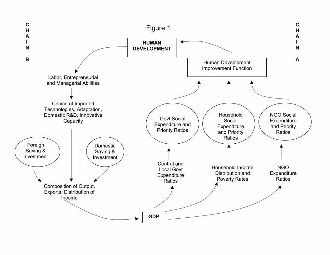
Figure 1

HUMAN DEVELOPMENT

GDP

NGO Expenditure

Ratios

NGO Social Expenditure and Priority

Ratios

Human Development Improvement Function

Household Social

Expenditure and Priority

Ratios

Govt Social Expenditure and Priority Ratios

Household Income Distribution and Poverty Rates

Central and Local Govt

Expenditure Ratios

Labor, Entrepreneurial and Managerial Abilities

Choice of Imported Technologies, Adaptation, Domestic R&D, Innovative

Capacity

Foreign Saving &

Investment

Domestic Saving &

Investment

Composition of Output, Exports, Distribution of

Income

C H A I N A

C H A I N B

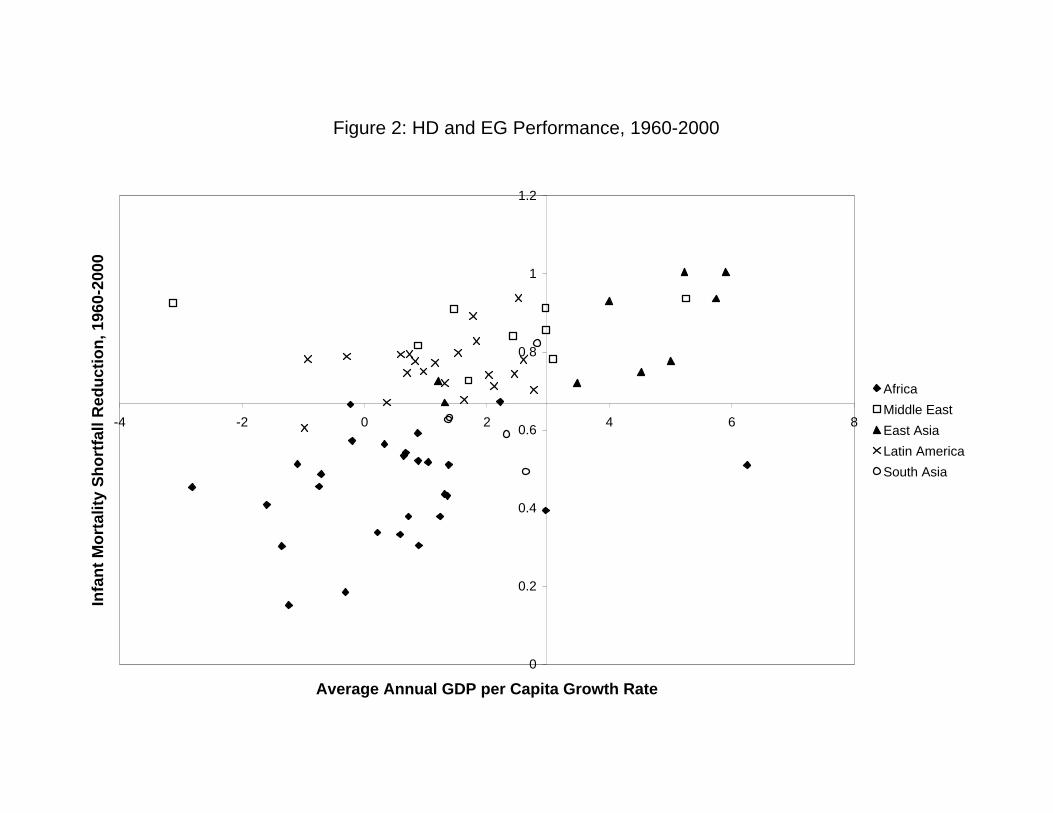
Figure 2: HD and EG Performance, 1960-2000

0

0.2

0.4

0.6

0.8

1

1.2

-4 -2 0 2 4 6 8

Average Annual GDP per Capita Growth Rate

Infa

nt

Mo

rtal

ity

Sh

ort

fall

Red

uct

ion

, 196

0-20

00

Africa

Middle East

East Asia

Latin America

South Asia

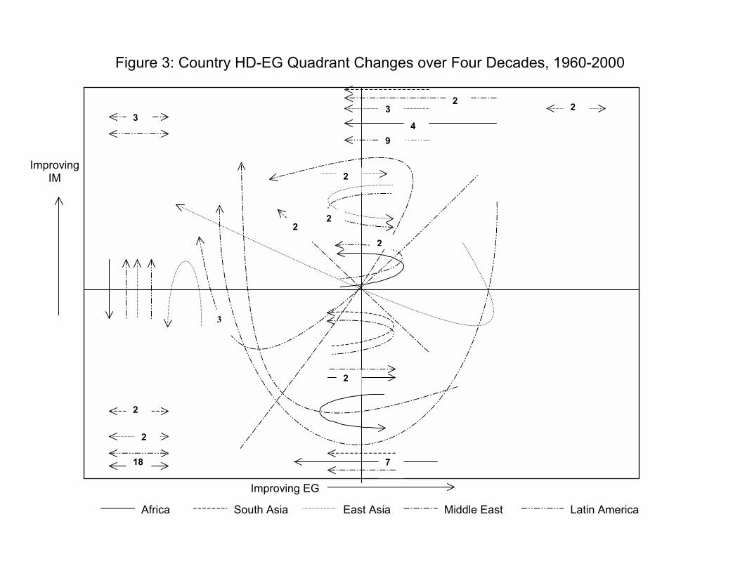
Figure 3: Country HD-EG Quadrant Changes over Four Decades, 1960-2000

7

Africa South Asia East Asia Middle East Latin America

Improving IM

Improving EG

18

2

3

2

2

2

3

2

2

9

2

2

3

2

4

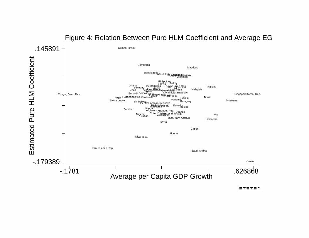
Figure 4: Relation Between Pure HLM Coefficient and Average EGE

stim

ated

Pur

e H

LM C

oeffi

cien

t

Average per Capita GDP Growth

-.1781 .626868-.179389

.145891

Senegal

Madagascar

Lesotho

Congo, Rep.

Guinea-Bissau

Somalia

Liberia

Sierra Leone

Cameroon

Central African Republic

Burkina Faso

Zambia

Mali

Rwanda

Cote d'Ivoire Uganda

Kenya

ChadBurundi

Mauritania

Ghana

Gambia

Malawi

Sudan

Zimbabwe

Nigeria

Gabon

Togo

Congo, Dem. Rep.

Botswana

Mauritius

Niger

Benin

Saudi Arabia

Oman

Tunisia

Syria

UAE

Algeria

Iraq

Egypt, Arab Rep.

Jordan

Kuwait

Morocco

Afghanistan

Turkey

Bangladesh

Korea, Rep.

Cambodia

Sri Lanka

Pakistan

India

Indonesia

Philippines

Iran, Islamic Rep.

Papua New Guinea

Nepal

ThailandMalaysia

Singapore

Colombia

Ecuador

Guatemala

Nicaragua

Venezuela

Trinidad and Tobago

Uruguay

Costa Rica

Bolivia

Panama

Argentina

Brazil

Jamaica

Haiti

HondurasMexico

Peru

Chile

Paraguay

El Salvador

Dominican Republic

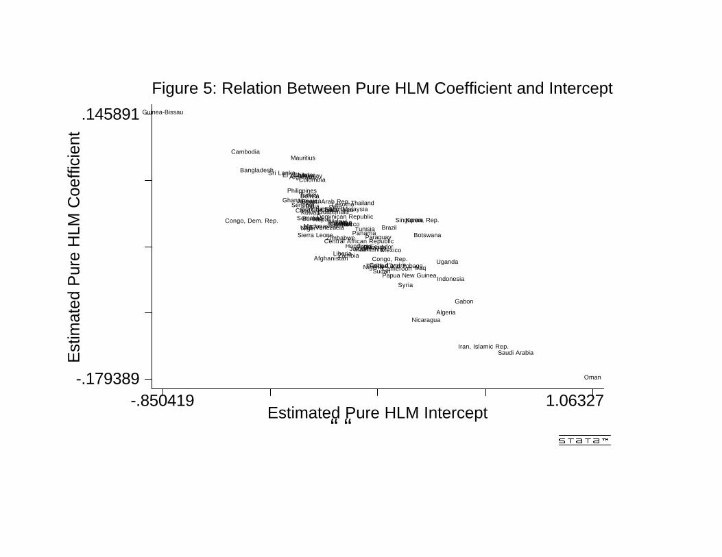
Figure 5: Relation Between Pure HLM Coefficient and InterceptE

stim

ated

Pur

e H

LM C

oeffi

cien

t

“ “Estimated Pure HLM Intercept

-.850419 1.06327-.179389

.145891

Senegal

Madagascar

Lesotho

Congo, Rep.

Guinea-Bissau

Somalia

Liberia

Sierra Leone

Cameroon

Central African Republic

Burkina Faso

Zambia

Mali

Rwanda

Cote d'Ivoire Uganda

Kenya

ChadBurundi

Mauritania

Ghana

Gambia

Malawi

Sudan

Zimbabwe

Nigeria

Gabon

Togo

Congo, Dem. Rep.

Botswana

Mauritius

Niger

Benin

Saudi Arabia

Oman

Tunisia

Syria

UAE

Algeria

Iraq

Egypt, Arab Rep.

Jordan

Kuwait

Morocco

Afghanistan

Turkey

Bangladesh

Korea, Rep.

Cambodia

Sri Lanka

Pakistan

India

Indonesia

Philippines

Iran, Islamic Rep.

Papua New Guinea

Nepal

ThailandMalaysia

Singapore

Colombia

Ecuador

Guatemala

Nicaragua

Venezuela

Trinidad and Tobago

Uruguay

Costa Rica

Bolivia

Panama

Argentina

Brazil

Jamaica

Haiti

HondurasMexico

Peru

Chile

Paraguay

El Salvador

Dominican Republic

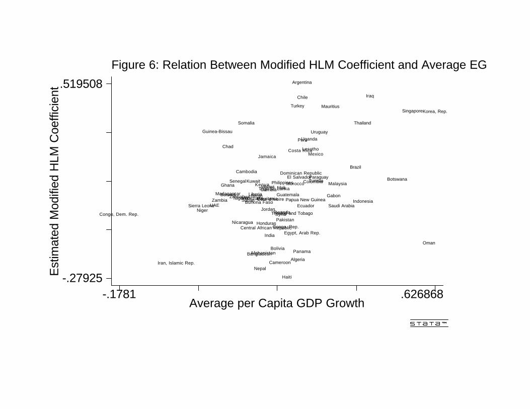
Figure 6: Relation Between Modified HLM Coefficient and Average EGE

stim

ated

Mod

ified

HLM

Coe

ffici

ent

Average per Capita GDP Growth

-.1781 .626868-.27925

.519508

Senegal

Madagascar

Lesotho

Congo, Rep.

Guinea-Bissau

Somalia

Liberia

Sierra Leone

Cameroon

Central African Republic

Burkina FasoZambia

Mali

Rwanda

Cote d'Ivoire

Uganda

Kenya

Chad

BurundiMauritania

GhanaGambiaMalawi

SudanZimbabweNigeria Gabon

Togo

Congo, Dem. Rep.

Botswana

Mauritius

Niger

Benin

Saudi Arabia

Oman

Tunisia

Syria

UAE

Algeria

Iraq

Egypt, Arab Rep.

Jordan

Kuwait Morocco

Afghanistan

Turkey

Bangladesh

Korea, Rep.

Cambodia

Sri Lanka

Pakistan

India

Indonesia

Philippines

Iran, Islamic Rep.

Papua New Guinea

Nepal

Thailand

Malaysia

Singapore

Colombia

Ecuador

Guatemala

Nicaragua

Venezuela

Trinidad and Tobago

Uruguay

Costa Rica

BoliviaPanama

Argentina

Brazil

Jamaica

Haiti

Honduras

Mexico

Peru

Chile

ParaguayEl SalvadorDominican Republic

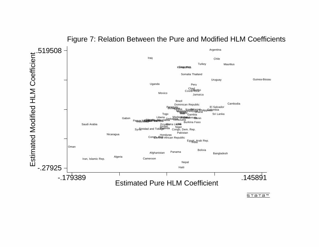
Figure 7: Relation Between the Pure and Modified HLM CoefficientsE

stim

ated

Mod

ified

HLM

Coe

ffici

ent

Estimated Pure HLM Coefficient

-.179389 .145891-.27925

.519508

Senegal

Madagascar

Lesotho

Congo, Rep.

Guinea-Bissau

Somalia

Liberia

Sierra Leone

Cameroon

Central African Republic

Burkina FasoZambia

Mali

Rwanda

Cote d'Ivoire

Uganda

Kenya

Chad

BurundiMauritania

GhanaGambia

Malawi

SudanZimbabweNigeriaGabon

Togo

Congo, Dem. Rep.

Botswana

Mauritius

Niger

Benin

Saudi Arabia

Oman

Tunisia

Syria

UAE

Algeria

Iraq

Egypt, Arab Rep.

Jordan

KuwaitMorocco

Afghanistan

Turkey

Bangladesh

Korea, Rep.

Cambodia

Sri Lanka

Pakistan

India

Indonesia

Philippines

Iran, Islamic Rep.

Papua New Guinea

Nepal

Thailand

Malaysia

Singapore

Colombia

Ecuador

Guatemala

Nicaragua

Venezuela

Trinidad and Tobago

Uruguay

Costa Rica

BoliviaPanama

Argentina

Brazil

Jamaica

Haiti

Honduras

Mexico

Peru

Chile

Paraguay El SalvadorDominican Republic

Figure 8: Explaining Sustainability of EG With IMM

odifi

ed H

LM C

oeffi

cien

t

Average Infant Mortality Rate

Africa

-.323197

.519508

Senegal

Namibia

Madagascar

Lesotho

Congo, Rep.

Guinea-BissauSomalia

LiberiaSierra Leone

Cameroon

Central African Republic

Burkina Faso ZambiaMali

Rwanda

Cote d'Ivoire

Uganda

Kenya

Chad

BurundiMauritania

GhanaGambiaMalawi

Sudan

Ethiopia

ZimbabweNigeriaGabonTogo

Congo, Dem. Rep.

Botswana

Mauritius

Niger

Benin

Middle East

Saudi Arabia

Oman

Tunisia

SyriaUAE

Algeria

Iraq

Libya

Egypt, Arab Rep.

Jordan

KuwaitMorocco

Asia

34.7462 70.7078-.323197

.519508

Afghanistan

Turkey

Bangladesh

Korea, Rep.

Cambodia

Sri Lanka

Pakistan

India

Indonesia

Philippines

Iran, Islamic Rep.

Papua New Guinea

Nepal

Thailand

Malaysia

Singapore

Latin America

34.7462 70.7078

Colombia

EcuadorGuatemala

Nicaragua

Venezuela

Trinidad and Tobago

Uruguay

Costa Rica

Bolivia Panama

Argentina

BrazilJamaica

Haiti

Honduras

Mexico

Peru

Chile

ParaguayEl SalvadorDominican Republic

Figure 9: Explaining Sustainiability of EG With LEM

odifi

ed H

LM C

oeffi

cien

t

Average Life Expectancy

Africa

-.323197

.519508

Senegal

Namibia

Madagascar

Lesotho

Congo, Rep.

Guinea-BissauSomalia

LiberiaSierra Leone

Cameroon

Central African Republic

Burkina Faso ZambiaMali

Rwanda

Cote d'Ivoire

Uganda

Kenya

Chad

BurundiMauritania

GhanaGambiaMalawi

Sudan

Ethiopia

ZimbabweNigeriaGabonTogo

Congo, Dem. Rep.

Botswana

Mauritius

Niger

Benin

Middle East

Saudi Arabia

Oman

Tunisia

SyriaUAE

Algeria

Iraq

Libya

Egypt, Arab Rep.

Jordan

KuwaitMorocco

Asia

34.7462 70.7078-.323197

.519508

Afghanistan

Turkey

Bangladesh

Korea, Rep.

Cambodia

Sri Lanka

Pakistan

India

Indonesia

Philippines

Iran, Islamic Rep.

Papua New Guinea

Nepal

Thailand

Malaysia

Singapore

Latin America

34.7462 70.7078

Colombia

EcuadorGuatemala

Nicaragua

Venezuela

Trinidad and Tobago

Uruguay

Costa Rica

Bolivia Panama

Argentina

BrazilJamaica

Haiti

Honduras

Mexico

Peru

Chile

ParaguayEl SalvadorDominican Republic

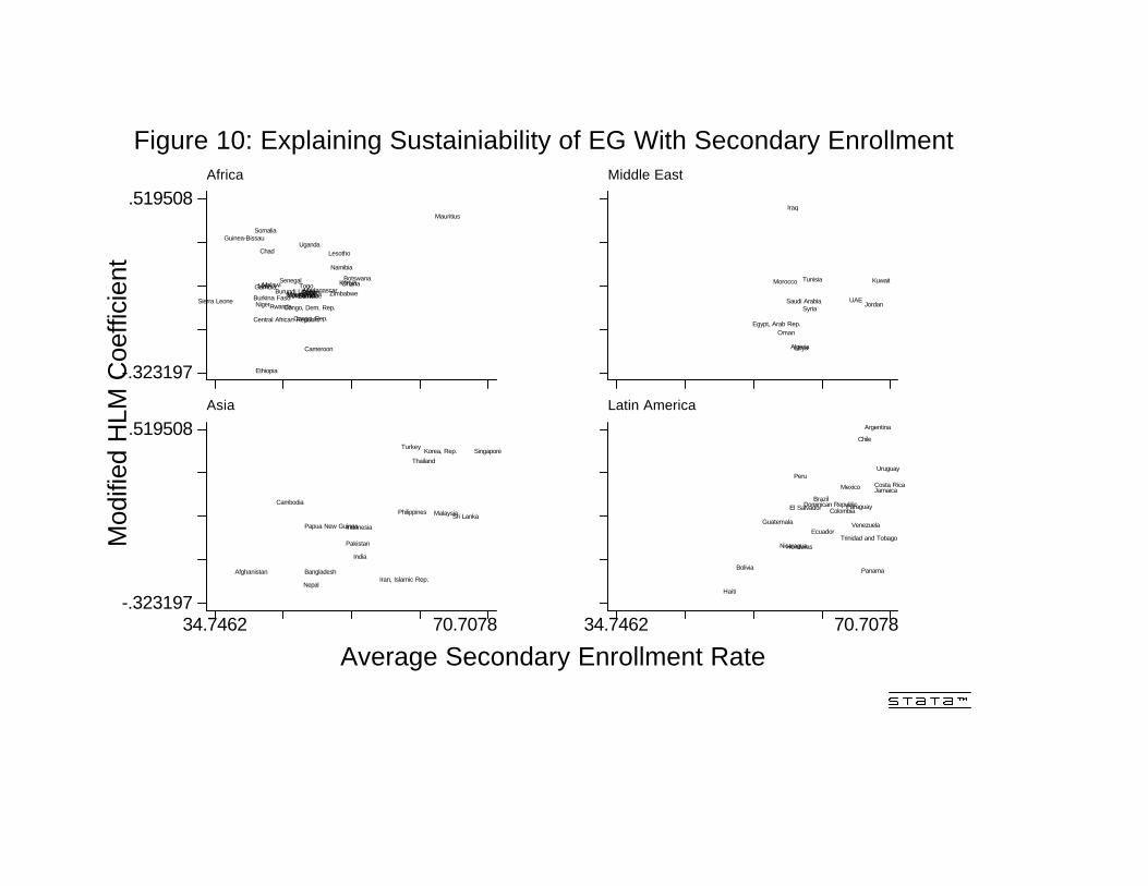
Figure 10: Explaining Sustainiability of EG With Secondary EnrollmentM

odifi

ed H

LM C

oeffi

cien

t

Average Secondary Enrollment Rate

Africa

-.323197

.519508

Senegal

Namibia

Madagascar

Lesotho

Congo, Rep.

Guinea-BissauSomalia

LiberiaSierra Leone

Cameroon

Central African Republic

Burkina Faso ZambiaMali

Rwanda

Cote d'Ivoire

Uganda

Kenya

Chad

BurundiMauritania

GhanaGambiaMalawi

Sudan

Ethiopia

ZimbabweNigeriaGabonTogo

Congo, Dem. Rep.

Botswana

Mauritius

Niger

Benin

Middle East

Saudi Arabia

Oman

Tunisia

SyriaUAE

Algeria

Iraq

Libya

Egypt, Arab Rep.

Jordan

KuwaitMorocco

Asia

34.7462 70.7078-.323197

.519508

Afghanistan

Turkey

Bangladesh

Korea, Rep.

Cambodia

Sri Lanka

Pakistan

India

Indonesia

Philippines

Iran, Islamic Rep.

Papua New Guinea

Nepal

Thailand

Malaysia

Singapore

Latin America

34.7462 70.7078

Colombia

EcuadorGuatemala

Nicaragua

Venezuela

Trinidad and Tobago

Uruguay

Costa Rica

Bolivia Panama

Argentina

BrazilJamaica

Haiti

Honduras

Mexico

Peru

Chile

ParaguayEl SalvadorDominican Republic

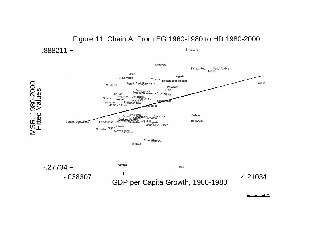
Figure 11: Chain A: From EG 1960-1980 to HD 1980-2000IM

SR

, 198

0-20

00F

itted

Val

ues

GDP per Capita Growth, 1960-1980

-.038307 4.21034-.27734

.888211

Afghanistan

Algeria

Argentina

Benin

Bolivia

Botswana

Brazil

Burkina Faso

Burundi

Cameroon

Central African RepublicChad

Chile

China

Colombia

Congo, Dem. Rep.

Costa Rica

Cote d'Ivoire

Dominican Republic

EcuadorEgypt, Arab Rep.

El Salvador

Gabon

Ghana

Guatemala

HaitiHonduras

India

Iraq

Jamaica

Kenya

Korea, Rep.

Lesotho

Liberia

Libya

MadagascarMalawi

Malaysia

Mauritania

Mauritius Mexico

Morocco

Nepal

Nicaragua

Niger

Nigeria

Oman

Pakistan

Panama

Papua New Guinea

ParaguayPeru

Philippines

Rwanda

Saudi Arabia

Senegal

Sierra Leone

Singapore

Somalia

Sri Lanka

Sudan

Syria

Thailand

Togo

Trinidad and TobagoTunisia

Uruguay

Venezuela

Zambia

Zimbabwe

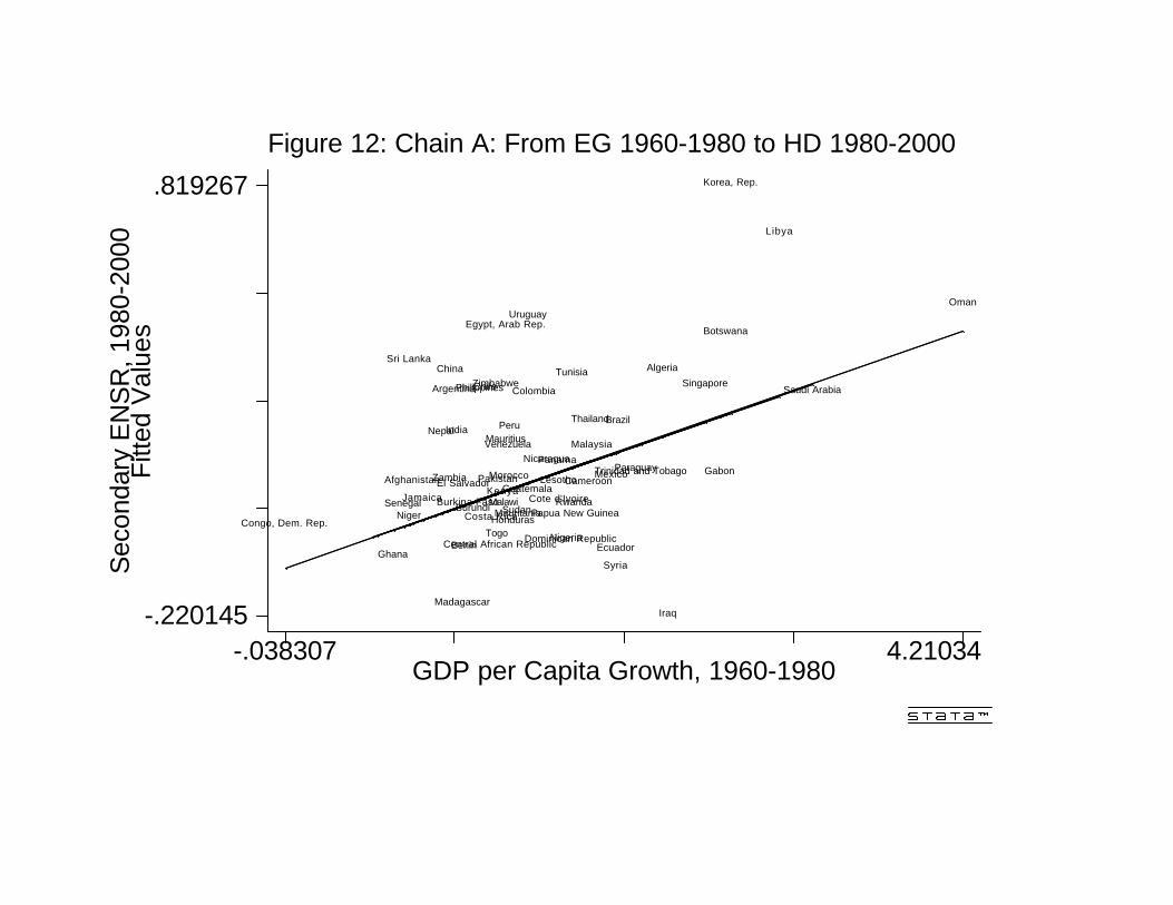
Figure 12: Chain A: From EG 1960-1980 to HD 1980-2000S

econ

dary

EN

SR

, 198

0-20

00F

itted

Val

ues

GDP per Capita Growth, 1960-1980

-.038307 4.21034-.220145

.819267

Afghanistan

Algeria

Argentina

Benin

Botswana

Brazil

Burkina FasoBurundi

Cameroon

Central African Republic

Chile

China

Colombia

Congo, Dem. Rep.Costa Rica

Cote d'Ivoire

Dominican RepublicEcuador

Egypt, Arab Rep.

El SalvadorGabon

Ghana

Guatemala

Honduras

India

Iraq

JamaicaKenya

Korea, Rep.

Lesotho

Libya

Madagascar

Malawi

Malaysia

Mauritania

Mauritius

MexicoMorocco

Nepal

Nicaragua

Niger

Nigeria

Oman

Pakistan

Panama

Papua New Guinea

Paraguay

Peru

Philippines

Rwanda

Saudi Arabia

Senegal

Singapore

Sri Lanka

Sudan

Syria

Thailand

Togo

Trinidad and Tobago

Tunisia

Uruguay

Venezuela

Zambia

Zimbabwe

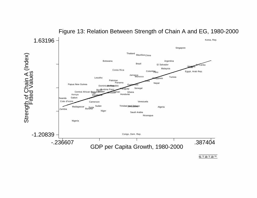
Figure 13: Relation Between Strength of Chain A and EG, 1980-2000S

treng

th o

f Cha

in A

(In

dex)

Fitt

ed V

alue

s

GDP per Capita Growth, 1980-2000

-.236607 .387404-1.20839

1.63196

Algeria

Argentina

Benin

BotswanaBrazil

Burkina Faso

Burundi

Cameroon

Central African Republic

Chile

China

Colombia

Congo, Dem. Rep.

Costa Rica

Cote d'Ivoire

Dominican Republic

Ecuador

Egypt, Arab Rep.

El Salvador

Gabon

Ghana

Guatemala

Honduras

India

Jamaica

Kenya

Korea, Rep.

Lesotho

Madagascar

Malawi

Malaysia

Mauritania

Mauritius

Mexico

Morocco

Nepal

Nicaragua

Niger

Nigeria

Oman

PakistanPanama

Papua New Guinea

Paraguay

Peru

Philippines

Rwanda

Saudi Arabia

Senegal

Singapore

Sri Lanka

SudanSyria

Thailand

Togo

Trinidad and Tobago

Tunisia

Uruguay

Venezuela

ZambiaZimbabwe

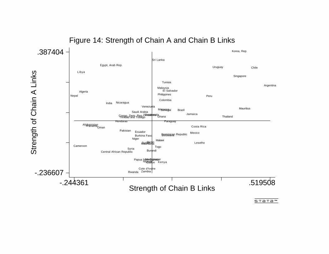
Figure 14: Strength of Chain A and Chain B LinksS

treng

th o

f Cha

in A

Lin

ks

Strength of Chain B Links

-.244361 .519508-.236607

.387404

Senegal

Madagascar

LesothoCameroon

Central African Republic

Burkina Faso

ZambiaRwandaCote d'Ivoire

Kenya

Burundi

Mauritania

Ghana

MalawiSudan

Zimbabwe

NigeriaGabon

Togo

Congo, Dem. Rep.

Botswana

Mauritius

NigerBenin

Saudi Arabia

Oman

Tunisia

Syria

Algeria

Libya

Egypt, Arab Rep.

Morocco

Afghanistan

Korea, Rep.

Sri Lanka

Pakistan

India

Philippines

Papua New Guinea

Nepal

Thailand

Malaysia

Singapore

Colombia

Ecuador

Guatemala

NicaraguaVenezuela

Trinidad and Tobago

Uruguay

Costa RicaPanama

Argentina

BrazilJamaica

Honduras

Mexico

Peru

Chile

Paraguay

El Salvador

Dominican Republic

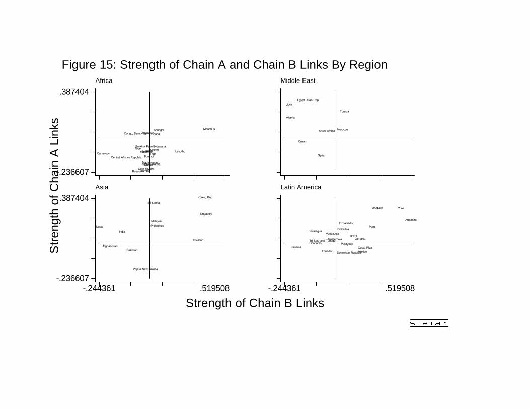
Figure 15: Strength of Chain A and Chain B Links By RegionS

treng

th o

f Cha

in A

Lin

ks

Strength of Chain B Links

Africa

-.236607

.387404

Senegal

Madagascar

LesothoCameroon

Central African Republic

Burkina Faso

ZambiaRwandaCote d'Ivoire

Kenya

BurundiMauritania

Ghana

MalawiSudan

Zimbabwe

NigeriaGabon

Togo

Congo, Dem. Rep.

Botswana

Mauritius

NigerBenin

Middle East

Saudi Arabia

Oman

Tunisia

Syria

Algeria

LibyaEgypt, Arab Rep.

Morocco

Asia

-.244361 .519508-.236607

.387404

Afghanistan

Korea, Rep.

Sri Lanka

Pakistan

India

Philippines

Papua New Guinea

Nepal

Thailand

Malaysia

Singapore

Latin America

-.244361 .519508

Colombia

Ecuador

Guatemala

NicaraguaVenezuela

Trinidad and Tobago

Uruguay

Costa RicaPanama

Argentina

BrazilJamaica

Honduras

Mexico

Peru

Chile

Paraguay

El Salvador

Dominican Republic

Table 1 Virtuous, Vicious and Lop-Sided Performance, 1960-2000

1960-1970

1970-1980

1980-1990

1990-2000

Africa Benin Vicious Vicious Vicious Vicious Botswana - Virtuous Virtuous HD-lopsided Burkina Faso Vicious Vicious Vicious Vicious Burundi EG-lopsided Vicious Vicious Vicious Cameroon Vicious EG-lopsided Vicious Vicious Central African Republic - Vicious Vicious Vicious Chad - Vicious Vicious Vicious Congo, Dem. Rep. Vicious Vicious Vicious Vicious Congo, Rep. Virtuous Virtuous Vicious Vicious Cote d'Ivoire EG-lopsided Vicious Vicious Vicious Eritrea - - - Vicious Ethiopia - - Vicious Vicious Gambia, The - - Vicious Vicious Ghana HD-lopsided Vicious Vicious Vicious Guinea-Bissau - - Vicious Vicious Kenya HD-lopsided Virtuous HD-lopsided HD-lopsided Lesotho EG-lopsided EG-lopsided Vicious Vicious Madagascar Vicious Vicious Vicious Vicious Malawi - EG-lopsided Vicious Vicious Mali - Vicious Vicious Vicious Mauritania - - Vicious Vicious Mauritius - - Virtuous HD-lopsided Mozambique - - Vicious EG-lopsided Namibia - - Vicious Vicious Niger - Vicious Vicious Vicious Nigeria EG-lopsided Vicious Vicious Vicious Rwanda Vicious Vicious Vicious Vicious Senegal Vicious Vicious Vicious Vicious

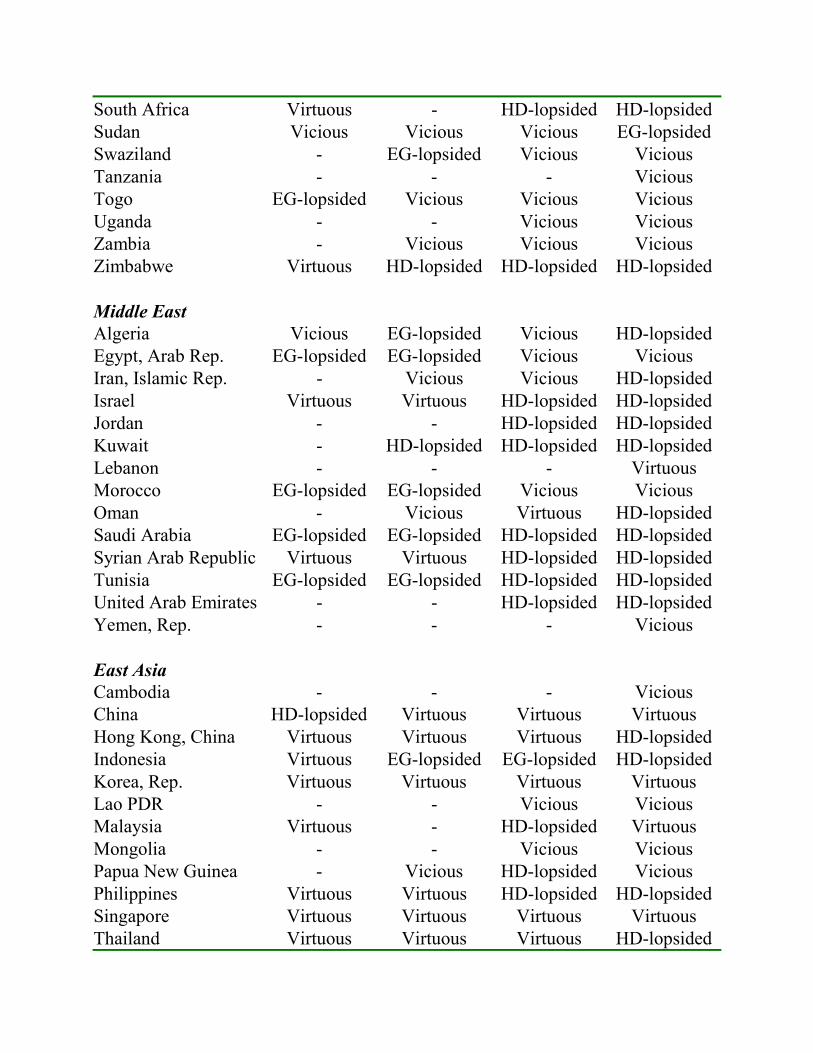
South Africa Virtuous - HD-lopsided HD-lopsided Sudan Vicious Vicious Vicious EG-lopsided Swaziland - EG-lopsided Vicious Vicious Tanzania - - - Vicious Togo EG-lopsided Vicious Vicious Vicious Uganda - - Vicious Vicious Zambia - Vicious Vicious Vicious Zimbabwe Virtuous HD-lopsided HD-lopsided HD-lopsided Middle East Algeria Vicious EG-lopsided Vicious HD-lopsided Egypt, Arab Rep. EG-lopsided EG-lopsided Vicious Vicious Iran, Islamic Rep. - Vicious Vicious HD-lopsided Israel Virtuous Virtuous HD-lopsided HD-lopsided Jordan - - HD-lopsided HD-lopsided Kuwait - HD-lopsided HD-lopsided HD-lopsided Lebanon - - - Virtuous Morocco EG-lopsided EG-lopsided Vicious Vicious Oman - Vicious Virtuous HD-lopsided Saudi Arabia EG-lopsided EG-lopsided HD-lopsided HD-lopsided Syrian Arab Republic Virtuous Virtuous HD-lopsided HD-lopsided Tunisia EG-lopsided EG-lopsided HD-lopsided HD-lopsided United Arab Emirates - - HD-lopsided HD-lopsided Yemen, Rep. - - - Vicious East Asia Cambodia - - - Vicious China HD-lopsided Virtuous Virtuous Virtuous Hong Kong, China Virtuous Virtuous Virtuous HD-lopsided Indonesia Virtuous EG-lopsided EG-lopsided HD-lopsided Korea, Rep. Virtuous Virtuous Virtuous Virtuous Lao PDR - - Vicious Vicious Malaysia Virtuous - HD-lopsided Virtuous Mongolia - - Vicious Vicious Papua New Guinea - Vicious HD-lopsided Vicious Philippines Virtuous Virtuous HD-lopsided HD-lopsided Singapore Virtuous Virtuous Virtuous Virtuous Thailand Virtuous Virtuous Virtuous HD-lopsided

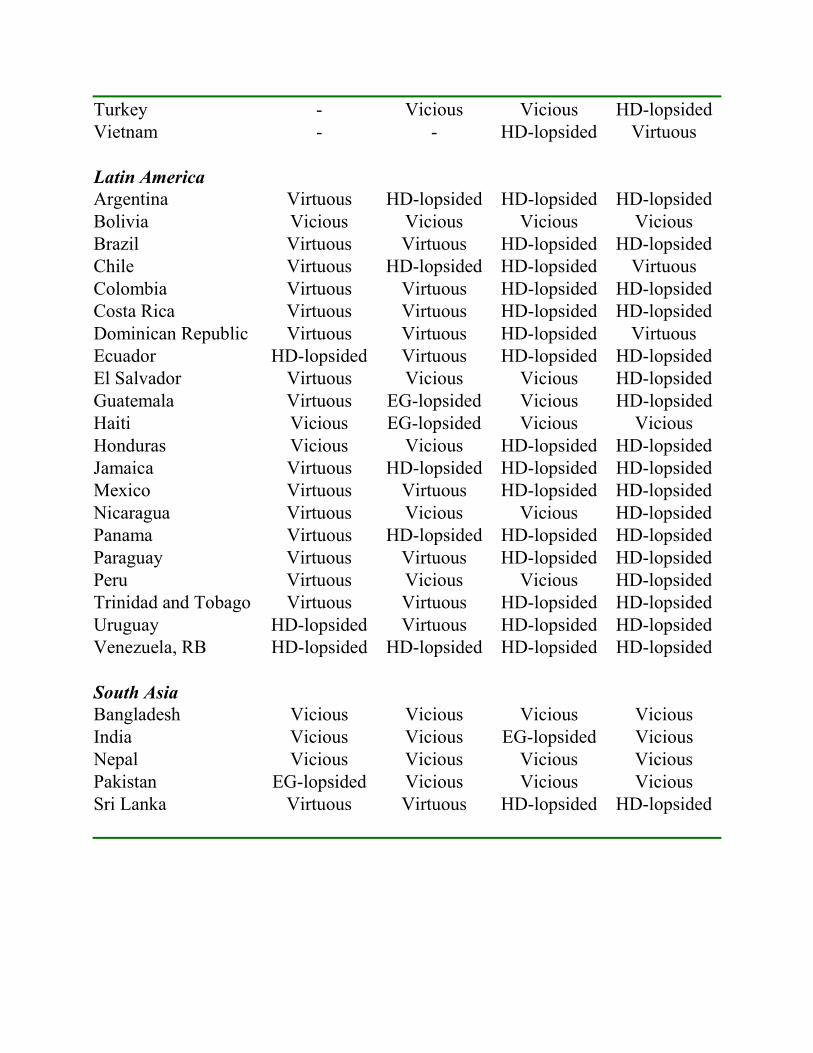
Turkey - Vicious Vicious HD-lopsided Vietnam - - HD-lopsided Virtuous Latin America Argentina Virtuous HD-lopsided HD-lopsided HD-lopsided Bolivia Vicious Vicious Vicious Vicious Brazil Virtuous Virtuous HD-lopsided HD-lopsided Chile Virtuous HD-lopsided HD-lopsided Virtuous Colombia Virtuous Virtuous HD-lopsided HD-lopsided Costa Rica Virtuous Virtuous HD-lopsided HD-lopsided Dominican Republic Virtuous Virtuous HD-lopsided Virtuous Ecuador HD-lopsided Virtuous HD-lopsided HD-lopsided El Salvador Virtuous Vicious Vicious HD-lopsided Guatemala Virtuous EG-lopsided Vicious HD-lopsided Haiti Vicious EG-lopsided Vicious Vicious Honduras Vicious Vicious HD-lopsided HD-lopsided Jamaica Virtuous HD-lopsided HD-lopsided HD-lopsided Mexico Virtuous Virtuous HD-lopsided HD-lopsided Nicaragua Virtuous Vicious Vicious HD-lopsided Panama Virtuous HD-lopsided HD-lopsided HD-lopsided Paraguay Virtuous Virtuous HD-lopsided HD-lopsided Peru Virtuous Vicious Vicious HD-lopsided Trinidad and Tobago Virtuous Virtuous HD-lopsided HD-lopsided Uruguay HD-lopsided Virtuous HD-lopsided HD-lopsided Venezuela, RB HD-lopsided HD-lopsided HD-lopsided HD-lopsided South Asia Bangladesh Vicious Vicious Vicious Vicious India Vicious Vicious EG-lopsided Vicious Nepal Vicious Vicious Vicious Vicious Pakistan EG-lopsided Vicious Vicious Vicious Sri Lanka Virtuous Virtuous HD-lopsided HD-lopsided

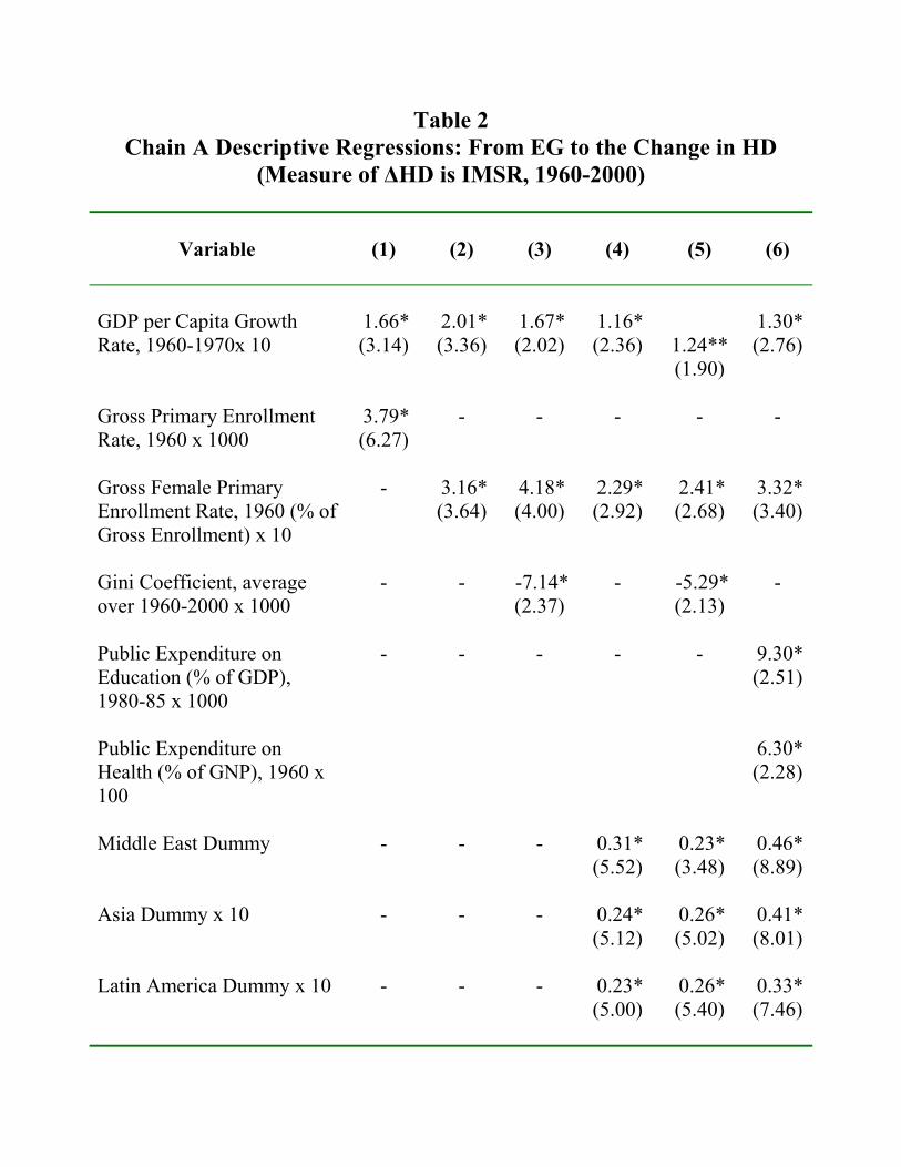
Table 2 Chain A Descriptive Regressions: From EG to the Change in HD

(Measure of ∆HD is IMSR, 1960-2000)

Variable

(1)

(2)

(3)

(4)

(5)

(6)

GDP per Capita Growth Rate, 1960-1970x 10

1.66* (3.14)

2.01* (3.36)

1.67* (2.02)

1.16* (2.36)

1.24** (1.90)

1.30* (2.76)

Gross Primary Enrollment Rate, 1960 x 1000

3.79* (6.27)

- - - - -

Gross Female Primary Enrollment Rate, 1960 (% of Gross Enrollment) x 10

- 3.16* (3.64)

4.18* (4.00)

2.29* (2.92)

2.41* (2.68)

3.32* (3.40)

Gini Coefficient, average over 1960-2000 x 1000

- - -7.14* (2.37)

- -5.29* (2.13)

-

Public Expenditure on Education (% of GDP), 1980-85 x 1000

- - - - - 9.30* (2.51)

Public Expenditure on Health (% of GNP), 1960 x 100

6.30* (2.28)

Middle East Dummy -

- - 0.31*

(5.52) 0.23* (3.48)

0.46* (8.89)

Asia Dummy x 10 -

- - 0.24*

(5.12) 0.26* (5.02)

0.41* (8.01)

Latin America Dummy x 10 -

- - 0.23*

(5.00) 0.26* (5.40)

0.33* (7.46)

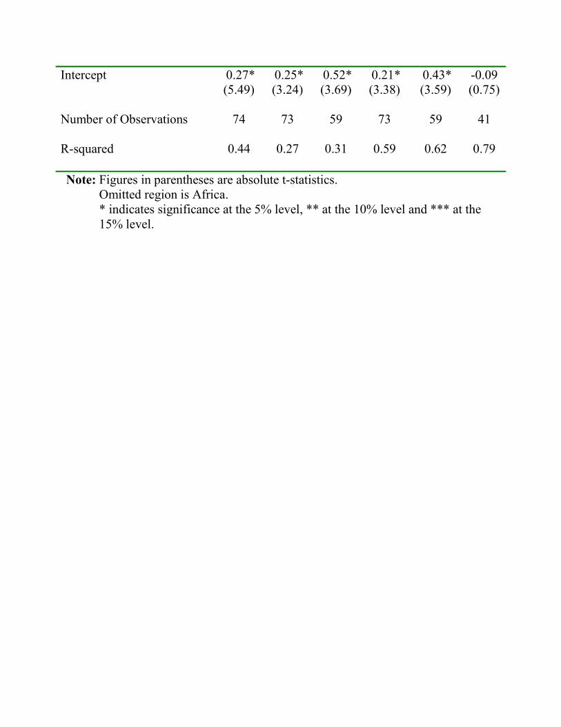
Intercept 0.27* (5.49)

0.25* (3.24)

0.52* (3.69)

0.21* (3.38)

0.43* (3.59)

-0.09 (0.75)

Number of Observations 74 73 59 73 59 41 R-squared 0.44 0.27 0.31 0.59 0.62 0.79 Note: Figures in parentheses are absolute t-statistics. Omitted region is Africa.

* indicates significance at the 5% level, ** at the 10% level and *** at the 15% level.

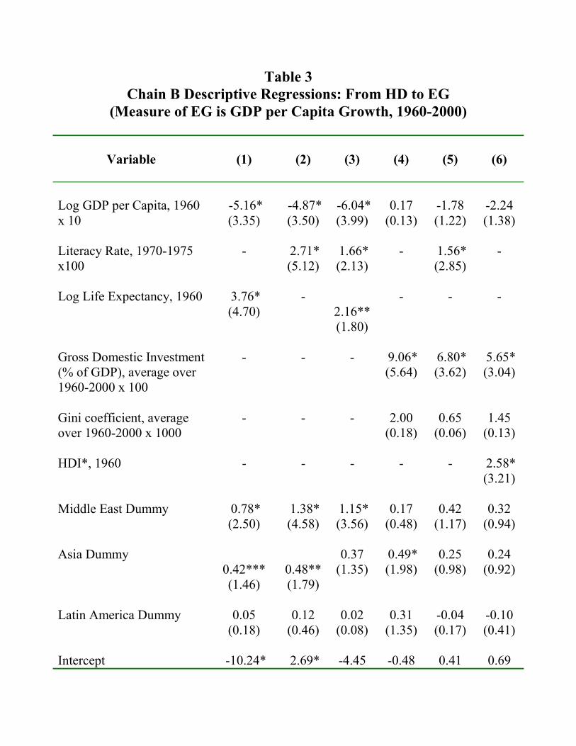
Table 3 Chain B Descriptive Regressions: From HD to EG

(Measure of EG is GDP per Capita Growth, 1960-2000)

Variable

(1)

(2)

(3)

(4)

(5)

(6)

Log GDP per Capita, 1960 x 10

-5.16* (3.35)

-4.87* (3.50)

-6.04* (3.99)

0.17 (0.13)

-1.78 (1.22)

-2.24 (1.38)

Literacy Rate, 1970-1975 x100

-

2.71* (5.12)

1.66* (2.13)

- 1.56* (2.85)

-

Log Life Expectancy, 1960 3.76*

(4.70) -

2.16** (1.80)

- - -

Gross Domestic Investment (% of GDP), average over 1960-2000 x 100

- - - 9.06* (5.64)

6.80* (3.62)

5.65* (3.04)

Gini coefficient, average over 1960-2000 x 1000

- - - 2.00 (0.18)

0.65 (0.06)

1.45 (0.13)

HDI*, 1960 - - - - - 2.58*

(3.21) Middle East Dummy 0.78*

(2.50) 1.38* (4.58)

1.15* (3.56)

0.17 (0.48)

0.42 (1.17)

0.32 (0.94)

Asia Dummy

0.42*** (1.46)

0.48** (1.79)

0.37 (1.35)

0.49* (1.98)

0.25 (0.98)

0.24 (0.92)

Latin America Dummy 0.05

(0.18) 0.12

(0.46) 0.02

(0.08) 0.31

(1.35) -0.04 (0.17)

-0.10 (0.41)

Intercept -10.24* 2.69* -4.45 -0.48 0.41 0.69

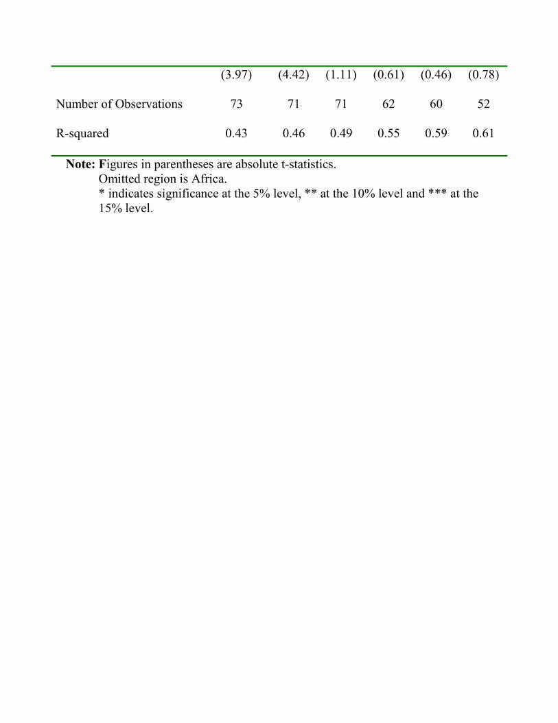
(3.97) (4.42) (1.11) (0.61) (0.46) (0.78) Number of Observations 73 71 71 62 60 52 R-squared 0.43 0.46 0.49 0.55 0.59 0.61

Note: Figures in parentheses are absolute t-statistics. Omitted region is Africa.

* indicates significance at the 5% level, ** at the 10% level and *** at the 15% level.

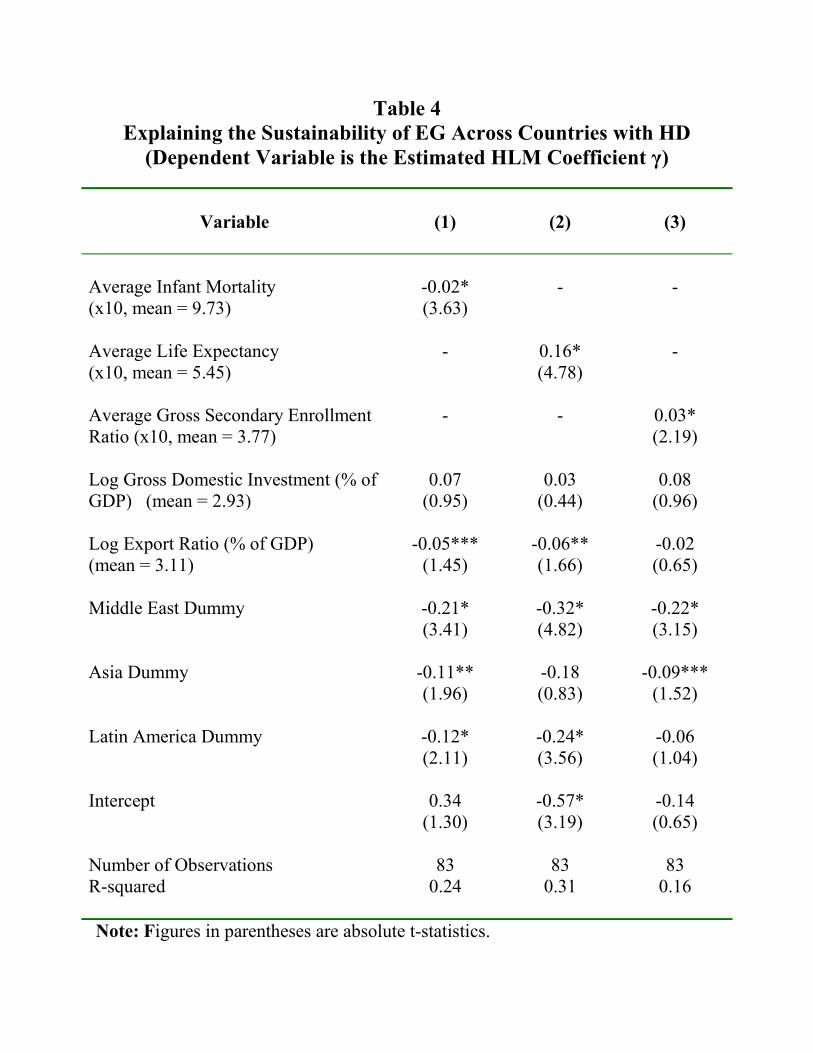
Table 4 Explaining the Sustainability of EG Across Countries with HD

(Dependent Variable is the Estimated HLM Coefficient γ)

Variable

(1)

(2)

(3)

Average Infant Mortality (x10, mean = 9.73)

-0.02* (3.63)

- -

Average Life Expectancy (x10, mean = 5.45)

-

0.16* (4.78)

-

Average Gross Secondary Enrollment Ratio (x10, mean = 3.77)

- - 0.03* (2.19)

Log Gross Domestic Investment (% of GDP) (mean = 2.93)

0.07 (0.95)

0.03 (0.44)

0.08 (0.96)

Log Export Ratio (% of GDP) (mean = 3.11)

-0.05*** (1.45)

-0.06** (1.66)

-0.02 (0.65)

Middle East Dummy -0.21*

(3.41) -0.32* (4.82)

-0.22* (3.15)

Asia Dummy -0.11**

(1.96) -0.18 (0.83)

-0.09*** (1.52)

Latin America Dummy -0.12*

(2.11) -0.24* (3.56)

-0.06 (1.04)

Intercept 0.34

(1.30) -0.57* (3.19)

-0.14 (0.65)

Number of Observations 83 83 83 R-squared 0.24 0.31 0.16 Note: Figures in parentheses are absolute t-statistics.