Path integrals for fermions, susy quantummechanics, etc..

(Appunti per il corso di Fisica Teorica 2 – 2012/13)

Fiorenzo Bastianelli

Fermions at the classical level can be described by Grassmann variables, also known asanticommuting or fermionic variables. These variables allow to introduce “classical” modelsthat upon quantization produce the degrees of freedom associated to spin. Actually, ratherthan “classical” models one should call them “pseudoclassical”, since the description of spin atthe classical level is a formal construction (spin vanish for ~ → 0). However, quantization ofGrassmann variables gives rise to spin degrees of freedom, and for simplicity we keep using theterm classical for such models.

In worldline approaches to quantum field theories, one often describes relativistic pointparticles with spin by using worldline coordinates for the position of the particle in space-timeand Grassmann variables to account for the associated spin degrees of freedom. From theworldline point of view these Grassmann variables have equations of motion that are first orderin time, and give rise to a Dirac equation in one dimension (the worldline can be considered as a0+1 dimensional space-time, with the one dimension corresponding to the time direction). Theyare fermions on the worldline and obey the Pauli exclusion principle, even though there is noreal spin in a zero dimensional space. In the following we study the path integral quantization ofmodels with Grassmann variables, and refer to them as path integrals for fermions, or fermionicpath integrals. In a hypercondensed notation the resulting formulae describe the quantizationof a Dirac field in higher dimensions as well.

Thus, we start introducing Grassmann variables and develop the canonical quantization ofmechanical models with Grassmann variables. Using a suitable definition of coherent statesthat mimics the standard definition of coherent states for the harmonic oscillator, we derive apath integral representation of the transition amplitude for fermionic systems. To exemplifythe use of Grassmann variables in mechanical models, we present a class of supersymmetricmodels, which allow us to introduce supersymmetry and related tools in one of their simplestrealization. Supersymmetry is a guiding principle of many worldline descriptions of relativisticfields, as we shall discuss in chapter 5. The N = 1 and N = 2 superspaces, the former used inworldline description of Dirac fields, are also briefly exposed.

1 Grassmann algebras

A n-dimensional Grassmann algebra G = θi is formed by generators θi with i = 1, ..., n thatsatisfy

θi, θj ≡ θiθj + θjθi = 0 . (1)

In particular any fixed generator squares to zero

θ2i = 0 (2)

suggesting already at the classical level the essence of the Pauli exclusion principle, accordingto which one cannot put two identical fermions in the same quantum state.

1

Functions of these Grassmann variables have a finite Taylor expansion (in fact they arereally defined by the latter). For example, for n = 1 there is only one Grassmann variable θand an arbitrary function is given by

f(θ) = f0 + f1θ (3)

where f0 and f1 are taken to be either real or complex numbers. Similarly, for n = 2 one has

f(θ1, θ2) = f0 + f1θ1 + f2θ2 + f3θ1θ2 . (4)

Terms with an even number of θ’s are called Grassmann even (or equivalently even, commuting,or bosonic). Terms with an odd number of θ’s are called Grassmann odd (or equivalently odd,anticommuting, or fermionic).

Derivatives with respect to Grassmann variables are very simple. As any function can beat most linear with respect to a fixed Grassmann variable, one has just to keep track of signs.Left derivatives are defined by removing the variable from the left of its Taylor expansion: forthe function f(θ1, θ2) given above

∂L∂θ1

f(θ1, θ2) = f1 + f3θ2 . (5)

Similarly, right derivatives are obtained by removing the variable from the right

∂R∂θ1

f(θ1, θ2) = f1 − f3θ2 (6)

where a minus sign emerges because one has first to commute θ1 past θ2.Equivalently, using Grassmann increments δθ, one may write

δf = δθ∂Lf

∂θ=∂Rf

∂θδθ (7)

which makes evident how to keep track of signs. If not specified otherwise, we use left derivativesand omit the corresponding subscript.

Integration can be defined, according to Berezin, to be identical with differentiation∫dθ ≡ ∂

∂θ. (8)

This definition has the virtue of producing a translational invariant measure, that is∫dθf(θ + η) =

∫dθf(θ) . (9)

This statement is easily proven by a direct calculation∫dθf(θ + η) =

∫dθ (f0 + f1(θ + η)) = f1 =

∫dθf(θ) . (10)

Grassmann variables can be defined to be either real or complex. A real variable satisfies

θ = θ (11)

2

with the bar indicating complex conjugation. For products of Grassmann variables the complexconjugate is defined to include an exchange of their ordered position

θ1θ2 = θ2θ1 (12)

so that the complex conjugate of the product of two real variables is purely imaginary

θ1θ2 = −θ1θ2 . (13)

It is iθ1θ2 that is real, as the complex conjugate of the imaginary unit carries the additionalminus sign to obtain a formally real object

iθ1θ2 = iθ1θ2 . (14)

Complex Grassmann variables η and η can always be decomposed in terms of two real Grass-mann variables θ1 and θ2 by setting

η =1√2

(θ1 + iθ2) , η =1√2

(θ1 − iθ2) . (15)

Having defined integration over Grassmann variables, we consider in more details the gaus-sian integration that is at the core of fermonic path integrals. For the case of a single realGrassmann variable θ the gaussian function is trivial, e−aθ

2= 1, as θ anticommutes with itself.

One needs at least two real Grassmann variables θ1 and θ2 to have a nontrivial exponentialfunction with an exponent quadratic in Grassmann variables

e−aθ1θ2 = 1− aθ1θ2 (16)

where a is either a real or a complex number. With the above definitions the corresponding“gaussian integral” is computed straghtforwardly∫

dθ1dθ2 e−aθ1θ2 = a . (17)

Defining the antisymmetric 2× 2 matrix

A =

(0 a−a 0

)(18)

one may rewrite the result of the Grassmann integration as∫dθ1dθ2 e

− 12θiA

ijθj = Pfaff(A) (19)

where Pfaff(A) is the pfaffian, the square root of the determinant of A. The latter is necessarilypositive definite for antisymmetric matrices. It is easy to see that this formula extends to aneven number n = 2m of real Grassmann variables, so that one may write∫

dnθ e−12θiA

ijθj = Pfaff(A) (20)

3

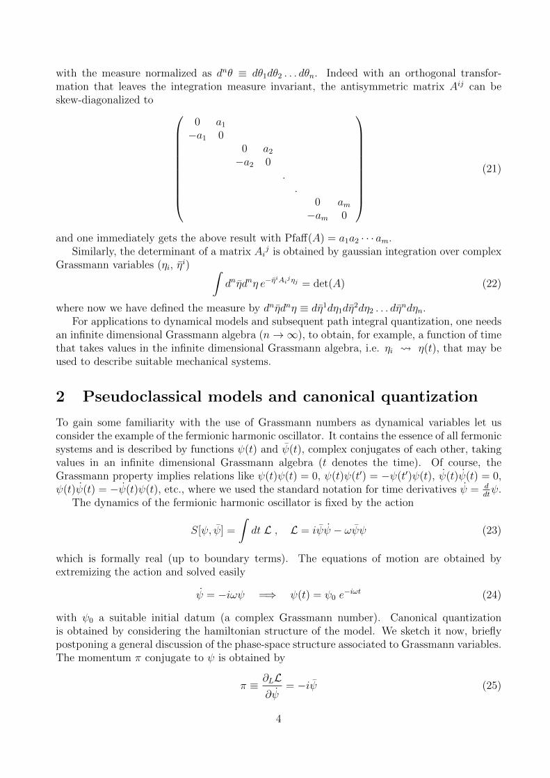
with the measure normalized as dnθ ≡ dθ1dθ2 . . . dθn. Indeed with an orthogonal transfor-mation that leaves the integration measure invariant, the antisymmetric matrix Aij can beskew-diagonalized to

0 a1

−a1 00 a2

−a2 0..

0 am−am 0

(21)

and one immediately gets the above result with Pfaff(A) = a1a2 · · · am.Similarly, the determinant of a matrix Ai

j is obtained by gaussian integration over complexGrassmann variables (ηi, η

i) ∫dnηdnη e−η

iAijηj = det(A) (22)

where now we have defined the measure by dnηdnη ≡ dη1dη1dη2dη2 . . . dη

ndηn.For applications to dynamical models and subsequent path integral quantization, one needs

an infinite dimensional Grassmann algebra (n→∞), to obtain, for example, a function of timethat takes values in the infinite dimensional Grassmann algebra, i.e. ηi η(t), that may beused to describe suitable mechanical systems.

2 Pseudoclassical models and canonical quantization

To gain some familiarity with the use of Grassmann numbers as dynamical variables let usconsider the example of the fermionic harmonic oscillator. It contains the essence of all fermonicsystems and is described by functions ψ(t) and ψ(t), complex conjugates of each other, takingvalues in an infinite dimensional Grassmann algebra (t denotes the time). Of course, theGrassmann property implies relations like ψ(t)ψ(t) = 0, ψ(t)ψ(t′) = −ψ(t′)ψ(t), ψ(t)ψ(t) = 0,ψ(t)ψ(t) = −ψ(t)ψ(t), etc., where we used the standard notation for time derivatives ψ = d

dtψ.

The dynamics of the fermionic harmonic oscillator is fixed by the action

S[ψ, ψ] =

∫dt L , L = iψψ − ωψψ (23)

which is formally real (up to boundary terms). The equations of motion are obtained byextremizing the action and solved easily

ψ = −iωψ =⇒ ψ(t) = ψ0 e−iωt (24)

with ψ0 a suitable initial datum (a complex Grassmann number). Canonical quantizationis obtained by considering the hamiltonian structure of the model. We sketch it now, brieflypostponing a general discussion of the phase-space structure associated to Grassmann variables.The momentum π conjugate to ψ is obtained by

π ≡ ∂LL∂ψ

= −iψ (25)

4

which shows that the systems is already in a hamiltonian form, the conjugate momenta beingψ up to factors. The classical Poisson bracket π, ψ

PB= −1 can be written as ψ, ψ

PB= −i.

Quantizing with anticommutators (as we shall see, fermionic system must be treated this way)one obtains

ψ, ψ† = ~ , ψ, ψ = ψ†, ψ† = 0 (26)

that is, the classical variables ψ, ψ are promoted to linear operators ψ, ψ† satisfying anticom-mutation relations taken to be i~ times the value of the classical Poisson brackets. Settingψ =√~ b and ψ† =

√~ b† one finds the fermionic creation/annihilation algebra

b, b† = 1 , b, b = b†, b† = 0 . (27)

The latter can be realized in a two dimensional Hilbert space. One may construct it a la Fock,considering b as destruction operator and b† as creation operator. One starts defining the Fockvacuum |0〉, fixed by the condition b|0〉 = 0. A second state is obtained acting with b†

|1〉 = b†|0〉 . (28)

No other states can be constructed acting with the creation operator b† as (b†)2 = 0. Nor-malizing the Fock vacuum to unity, 〈0|0〉 = 1, with 〈0| = |0〉†, one finds that these states areorthonomal

〈m|n〉 = δmn m,n = 0, 1 (29)

and span a two-dimensional Hibert space.Hamiltonian structure and canonical quantizationPath integrals for fermions can be derived form the canonical formalism, just as in the

bosonic case. For this we need to review briefly the hamiltonian formalism and canonicalquantization of mechanical systems with Grassmann variables.

The hamiltonian formalism aims to produce equations of motion as first order differentialequations in time. For a simple bosonic model with phase space coordinates (x, p), the phasespace action is usually written in the form

S[x, p] =

∫dt(px−H(x, p)

)(30)

The first term with derivatives (px) is called the symplectic term, and fixes the Poisson bracketstructure of phase space. Up to boundary terms it can be written in a more symmetrical form,with the time derivatives shared equally by x and p,

S[x, p] =

∫dt(1

2(px− xp) +H(x, p)

)=

∫dt(1

2za(Ω−1)abz

b +H(z))

(31)

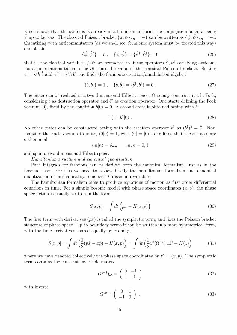
where we have denoted collectively the phase space coordinates by za = (x, p). The symplecticterm contains the constant invertible matrix

(Ω−1)ab =

(0 −11 0

)(32)

with inverse

Ωab =

(0 1−1 0

). (33)

5

The latter is used to define the Poisson bracket between generic phase space functions F andG

F,GPB

=∂F

∂zaΩab ∂G

∂zB(34)

which is readly seen to coincide with standard definitions. It satisfies the following properties:

F,GPB

= −G,FPB

(antisymmetry)

F,GHPB

= F,GPBH +GF,H

PB(Leibniz rule) (35)

F, G,HPBPB

+ G, H,FPBPB

+ H, F,GPBPB

= 0 (Jacobi identity)

These properties make it consistent to adopt the canonical quantization rules of substitutingthe fundamental variables za by linear operators za acting on a Hilbert space of physical states.The commutation relations of the za are fixed to be i~ times the value of the classical Poissonbrackets

[za, zb] = i~Ωab . (36)

More generally, phase space functions F (z) are elevated to operators F (z) (after fixing eventualordering ambiguities) having commutation relations with other operators of the form

[F (z), G(z)] = i~F,GPB

+ higher order terms in ~ . (37)

These prescriptions are consistent as both sides satisfy the same algebraic properties.This set up is readily extended to models containing Grassmann variables, after taking

care of sign arising from the anticommuting sector. We denote collectively the phase spacecoordinates by ZA = (xi, pi, θ

α), with (xi, pi) usual Grassmann even phase space variables andθα Grassmann odd variables. We consider a phase space action of the form

S[zA] =

∫dt

(1

2zA(Ω−1)AB z

B −H(z)

)(38)

where the symplectic term depends on a constant invertible matrix (Ω−1)AB with inverse ΩAB.Again this term must be written splitting the time derivatives democratically between allvariables, as in (31). The symplectic term as well as the hamiltonian are taken to be Grassmanneven (i.e. commuting objects). Then, it is seen that ΩAB is a truly antisymmetric matrix alongbosonic coordinates, while it is symmetric along anticommuting directions. It is used to definethe Poisson bracket by

F,GPB

=∂RF

∂zAΩAB ∂LG

∂zB(39)

where both right and left derivatives are used. In particular one finds ZA, ZBPB

= ΩAB. Forphase space functions F with definite Grassmann parity (−1)εF (εF = 0 if F is Grassmanneven, and εF = 1 if F is Grassmann odd), one finds a graded generalization of the propertiesin eq. (35), namely

F,GPB

= (−1)εF εG+1G,FPB

F,GHPB

= F,GPBH + (−1)εF εGGF,H

PB(40)

F, G,HPBPB

+ (−1)εF (εG+εH)G, H,FPBPB

+ (−1)εH(εF+εG)H, F,GPBPB

= 0

These properties make it consistent to adopt the canonical quantization rules of promotingphase space coordinates ZA to operators ZA with commutation/anticommutation rules fixedby the classical Poisson brackets

[ZA, ZB = i~ZA, ZBPB

= i~ΩAB (41)

6

where we have employed the compact notation

[· , · =

· , · anticommutator if both variables are fermionic

[· , ·] commutator otherwise(42)

The previous quick exposition becomes clearer by considering the following examples.

Examples

(i) Single real Grassmann variable ψ (single Majorana fermion in one dimension).Taking as phase space lagrangian

L =i

2ψψ −H(ψ) (43)

one finds Ω−1 = i, Ω = −i, and Poisson bracket at equal times ψ, ψPB

= −i. The dynamicalvariable ψ(t) is often called Majorana fermion in one dimension, as it satisfy a reality condition(akin to the Majorana condition) and the Dirac equation in one dimension. One may noticethat the only possible Grassmann even hamiltonian is a real constant. Also one verifies in thisexample that phase space can be odd dimensional if Grassmann variables are present. Thismodel is quantized by the anticommutator

ψ, ψ = ~ , (44)

however the quantum theory is trivial, as one may realize this algebra in a one dimensionalHilbert space, with the operator ψ acting as multiplication by

√~/2.

(ii) Several real Grassmann variables ψi (Majorana fermions in one dimension).For the case os several real Grassmann variables one may take as phase space lagrangian

L =i

2ψiψi −H(ψi) i = 1, ..., n (45)

and one finds (Ω−1)ij = iδij, Ωij = −iδij. Thus the Poisson brackets at equal times read asψi, ψj

PB= −iδij. Quantization is obtained by the anticommutator

ψi, ψj = ~δij (46)

which is recognized to be proportional to the Clifford algebra of the gamma matrices of theDirac equation in n euclidean dimensions. Indeed setting ψi =

√~/2 γi one finds γi, γj = 2δij

which is the defining properties of the gamma matrices appearing in the Dirac equation

(γi∂i +m)Ψ(x) = 0 . (47)

It is known that the algebra (46) is realized in a complex vector space of dimension 2[n2

], where[n

2] indicates the integer part of n

2. The previous case is recognized as a subcase of the present

one.(iii) Complex Grassmann variables ψ and ψ (Dirac fermion in one dimension).

Taking as phase space lagrangian

L = iψψ −H(ψ, ψ) (48)

7

one finds ψ, ψPB

= −i as the only nontrivial Poisson bracket between phase space coordinates

(ψ, ψ). It is quantized by the anticommutator ψ, ψ† = ~, producing a fermionic annihila-tion/creation algebra. It is realized in a two dimensional Fock space, as anticipated for the caseof the fermionic harmonic oscillator.

This basic result can be used to understand the statement on the dimensions of the gammamatrices. In even n = 2m dimensions one may combine the 2m Majorana fermions correspond-ing to the gamma matrices in m pairs of Dirac fermions, that generate a set of m independent,anticommuting annihilation/creation operators. The latter act on the m-th tensor product oftwo dimensional fermionic Fock spaces, giving a total Hilbert space of 2m dimensions, in accordwith the assertion given in point (ii) above. Adding an extra Majorana fermion to this set upcorresponds to a Clifford algebra in odd dimensions (2m + 1): the dimension of the Hilbertspace does not change and the last Majorana fermion can be realized as proportional to thechirality matrix of the 2m dimensional case.

2.1 Coherent states

For a derivation of the path integral for fermionic systems it is useful to introduce coherentstates, an overcomplete basis of vectors of the Fock space described previously. It is useful toreview the bosonic construction, to have a guide on the construction for the fermionic case.

In the theory of the harmonic oscillator one introduces coherent states defined as eigenstatesof the annihilation operator a. Let us recall that the algebra of the creation and annihilationoperators a† and a is the following

[a, a†] = 1 , [a, a] = 0 , [a†, a†] = 0 . (49)

It is realized in an infinite dimensional Hilbert space that can be identified with a Fock spacethrough the Fock construction, which goes as follows. A complete orthonormal basis is con-structed by starting from the Fock vacuum |0〉, defined by the condition a|0〉 = 0. The otherstates of the basis are obtained by acting with a† an arbitrary number of times on the Fockvacuum |0〉

|0〉 such that a|0〉 = 0

|1〉 = a†|0〉

|2〉 =a†√

2|1〉 =

(a†)2

√2!|0〉

|3〉 =a†√

3|2〉 =

(a†)3

√3!|0〉

...

|n〉 =a†√n|n− 1〉 =

(a†)n√n!|0〉

... (50)

Normalizing the Fock vacuum to unit norm, 〈0|0〉 = 1, where 〈0| = |0〉†, one finds that thesestates are orthonomal (it is enough to use the algebra (49) to verify it)

〈m|n〉 = δmn m,n = 0, 1, 2, ... . (51)

Now, choosing a complex number α, one builds the coherent states |α〉 as

|α〉 = eαa†|0〉 (52)

8

which turn out to be eigenstates of the annihilation operator a

a|α〉 = α|α〉 . (53)

A quick way of seeing this is by expanding the exponential and viewing |α〉 as an infinite sumwith suitable coefficients of the basis vectors constructed above

|α〉 = eαa†|0〉

=(

1 + αa† +1

2!(αa†)2 +

1

3!(αa†)3 + · · ·+ 1

n!(αa†)n + · · ·

)|0〉

= |0〉+ α|1〉+α2

√2!|2〉+

α3

√3!|3〉+ · · ·+ αn√

n!|n〉+ · · · . (54)

In this form it is easy to calculate (using a|n〉 =√n|n− 1〉)

a|α〉 = a(|0〉+ α|1〉+

α2

√2!|2〉+

α3

√3!|3〉+ · · ·+ αn√

n!|n〉+ · · ·

)= 0 + α|0〉+ α2|1〉+

α3

√2!|2〉+ · · ·+ αn√

(n− 1)!|n− 1〉+ · · ·

= α(|0〉+ α|1〉+

α2

√2!|2〉+ · · ·+ αn−1√

(n− 1)!|n− 1〉+ · · ·

)= α|α〉 . (55)

An even faster way is to realize that the algebra (49) can be realized by

a† → a , a → ∂

∂a(56)

with a ∈ C, and the result follows straighfowardly.A list of properties that can be easily proven with similar calculations are

(i) 〈α| = |α〉† = 〈0|eαa =⇒ 〈α|a† = 〈α|α(ii) 〈α|α〉 = eαα (scalar product)

(iii) 1 =

∫dαdα

2πie−αα |α〉〈α| (resolution of the identity)

(iv) Tr A =

∫dαdα

2πie−αα 〈α|A|α〉 (trace of the operator A) . (57)

One should note that the set of coherent states form an over-complete basis, it is not orthonor-mal (as 〈β|α〉 = eβα 6= 0), but it is useful to keep this redundancy.

A similar construction can be introduced for fermionic systems. Let us consider the algebraof the anticommutators of the fermionic creation and annihilation operators ψ† and ψ,

ψ, ψ† = 1 , ψ, ψ = 0 , ψ†, ψ† = 0 . (58)

This algebra can be realized by 2 × 2 matrices acting in the two-dimensional fermionic Fockspace generated by the vectors |0〉 and |1〉, defined by

ψ|0〉 = 0 , |1〉 = ψ†|0〉 . (59)

9

Indeed acting again with the fermionic creation operator on the state |1〉, does not produceadditional states (ψ†|1〉 = (ψ†)2|0〉 = 0 as a consequence of the algebra (58): one cannot haveoccupation numbers bigger then one. As already mentioned, this embodies the Pauli exclusionprinciple.

One defines fermionic coherent states again as eigenstates |ψ〉 of the annihilation operatorψ, having as eigenvalues the complex Grassmann number ψ

ψ|ψ〉 = ψ|ψ〉 . (60)

The Grassmann numbers, such as ψ and its complex conjugate ψ, anticommute of coursebetween themselves, and we define them to anticommute also with the fermionic operators ψ†

and ψ. No confusion should arise between the operators ψ and ψ† that have a hat, and thecomplex Grassmann variables ψ and ψ, egeinvalues of the eigenstates |ψ〉 and 〈ψ| respectively,that carry no hat (just as in the previous chapter we indicated position operator, eigenstatesand eigenvalues so that x|x〉 = x|x〉.)

One can prove the following properties

(i) |ψ〉 = eψ†ψ|0〉

(ii) 〈ψ| = 〈0|eψψ =⇒ 〈ψ|ψ† = 〈ψ|ψ

(iii) 〈ψ|ψ〉 = eψψ

(iv) 1 =

∫dψdψ e−ψψ |ψ〉〈ψ|

(v) Tr A =

∫dψdψ e−ψψ 〈−ψ|A|ψ〉

(vi) Str A = Tr[(−1)F A] =

∫dψdψ e−ψψ 〈ψ|A|ψ〉 . (61)

The proofs can be obtained by explicit calculation. Let us proceed systematically.(i) First of all one can expand the exponential and write the coherent state in the following

fashion

|ψ〉 = eψ†ψ|0〉

= (1 + ψ†ψ)|0〉 = |0〉 − ψψ†|0〉= |0〉 − ψ|1〉 (62)

so that one may compute

ψ|ψ〉 = ψeψ†ψ|0〉

= ψ(|0〉 − ψ|1〉

)= −ψψ|1〉 = ψψ|1〉 = ψ|0〉 = ψ

(|0〉 − ψ|1〉

)= ψ|ψ〉 (63)

which proves that |ψ〉 is a coherent state. Note that terms proportional to ψ2 can be insertedor eliminated at wish, as they vanish due to Grassmann property ψ2 = 0.

(ii) “Bra” coherent state. To prove this relation for a bra coherent state it is sufficientto take the hermitian conjugate of the ket coherent state |ψ〉. One must remember that the

10

definition of hermitian conjugate reduces to complex conjugation for Grassmann variables andincludes an exchange of the ordered position of both variables and operators. For example

(ψ†ψ)† = ψψ . (64)

(iii) Scalar product. It is sufficient to compute it directly (recalling that ψ2 = 0, ψ2 = 0and ψψ = −ψψ)

〈ψ|ψ〉 =(〈0| − 〈1|ψ

)(|0〉 − ψ|1〉

)= 〈0|0〉+ ψψ〈1|1〉 = 1 + ψψ

= eψψ . (65)

(iv) Resolution of the identity. First of all one must recall that the definition of integrationover Grassmann variables makes it identical with differentiation. In particular we use leftdifferentiation, that removes the variable form the left (one must pay attention to signs arisingfrom this operation) ∫

dψ ≡ ∂L∂ψ

,

∫dψ ≡ ∂L

∂ψ. (66)

Now a direct calculation shows that∫dψdψ e−ψψ |ψ〉〈ψ| =

∫dψdψ (1− ψψ)

(|0〉 − ψ|1〉

)(〈0| − 〈1|ψ

)= |0〉〈0|+ |1〉〈1| . (67)

We point out that the Grassmann variables are here defined to commute with the Fock vacuum|0〉, so that they commute with the coherent states, but anticommute with |1〉 = ψ†|0〉 (as theyanticommute with ψ†).

(v) Trace. Given a bosonic operator A, that commutes with ψ and ψ, one can verify that∫dψdψ e−ψψ 〈−ψ|A|ψ〉 =

∫dψdψ (1− ψψ)

(〈0|+ 〈1|ψ

)A(|0〉 − ψ|1〉

)=

∫dψdψ (1− ψψ)

(〈0|A|0〉 − ψψ〈1|A|1〉+ · · ·

)= 〈0|A|0〉+ 〈1|A|1〉= Tr A . (68)

(vi) Supertrace. An analogous calculation gives∫dψdψ e−ψψ 〈ψ|A|ψ〉 =

∫dψdψ (1− ψψ)

(〈0| − 〈1|ψ

)A(|0〉 − ψ|1〉

)=

∫dψdψ (1− ψψ)

(〈0|A|0〉+ ψψ〈1|A|1〉+ · · ·

)= 〈0|A|0〉 − 〈1|A|1〉 = Tr[(−1)F A]

= Str A . (69)

Here F is the fermion number operator (or occupation number, with egenvalues F = 0 for |0〉and F = 1 for |1〉). The last but one line indeed gives the definition of the supertrace.

11

3 Fermionic path integrals

We now have all the tools to find a path integral representation of the transition amplitude be-tween coherent states 〈ψf |e−iHT |ψi〉. We consider an hamiltonian H = H(ψ†, ψ) written in sucha way that all creation operators are on the left of the annihilation operators, something thatis always possible to achieve using the fundamental anticommutation relations in (58); indeedfor a single pair of fermionic creation and annihilation operators the most general (bosonic)hamiltonian is of the form H = ωψ†ψ + ω0.

First of all one divides the total propagation time T in N elementary steps of durationε = T

N, so that T = Nε. Using N − 1 times the decomposition of identity in terms of coherent

states one obtains the following equalites

〈ψf |e−iHT |ψi〉 = 〈ψf |(e−iHε

)N|ψi〉 = 〈ψf | e−iHεe−iHε · · · e−iHε︸ ︷︷ ︸

N volte

|ψi〉

= 〈ψf |e−iHε 1 e−iHε 1 · · · 1 e−iHε|ψi〉

=

∫ (N−1∏k=1

dψkdψk e−ψkψk

) N∏k=1

〈ψk|e−iHε|ψk−1〉 (70)

where we have defined ψ0 ≡ ψi and ψN ≡ ψf . For ε→ 0 one can approximate the elementarytransition amplitudes as follows

〈ψk|e−iH(ψ†,ψ)ε|ψk−1〉 = 〈ψk|(

1− iH(ψ†, ψ)ε+ · · ·)|ψk−1〉

= 〈ψk|ψk−1〉 − iε〈ψk|H(ψ†, ψ)|ψk−1〉+ · · ·

=(

1− iεH(ψk, ψk−1) + · · ·)〈ψk|ψk−1〉

= e−iεH(ψk,ψk−1)〈ψk|ψk−1〉= e−iεH(ψk,ψk−1)eψkψk−1 . (71)

The substitution H(ψ†, ψ)→ H(ψk, ψk−1) follows form the ordering of the hamiltonian that wehave specified previously (ψ† on the left and ψ on the right). This allows one to act with thecreation operator on the left on one of his eigenstates, and with the annihilation operator onthe right on one of his eigenstates, so that all operators in the hamitonian gets substituted bythe respective eigenvalues, producing a function of these Grassmann numbers. In this way thehamiltonian operator H(ψ†, ψ) is substituted by the hamiltonian function H(ψk, ψk−1). Theseapproximations are valid for N →∞, i.e. ε→ 0. Substituting (71) in (70) one gets

〈ψf |e−iHT |ψi〉 = limN→∞

∫ (N−1∏k=1

dψkdψk e−ψkψk

)ei

∑Nk=1[−iψkψk−1−H(ψk,ψk−1)ε]

= limN→∞

∫ (N−1∏k=1

dψkdψk

)ei

∑Nk=1[iψk(ψk−ψk−1)−H(ψk,ψk−1)ε]eψNψN

= limN→∞

∫ (N−1∏k=1

dψkdψk

)ei

∑Nk=1[iψk

(ψk−ψk−1)

ε−H(ψk,ψk−1)]ε+ψNψN

=

∫DψDψ ei

∫ T0 dt[iψψ−H(ψ,ψ)]+ψ(T )ψ(T ) =

∫DψDψ eiS[ψ,ψ] . (72)

12

This the path integral for one complex fermionic degree of freedom. We recognize in theexponent a discretization of the classical action

S[ψ, ψ] =

∫ T

0

dt [iψψ −H(ψ, ψ)]− iψ(T )ψ(T )

→N−1∑k=1

[iψk(ψk − ψk−1)

ε−H(ψk, ψk−1)]ε− iψNψN (73)

where T = Nε is the total propagation time. The last way of writing the amplitude in (72)is symbolic and indicates the formal sum over all paths ψ(t), ψ(t) such that ψ(0) = ψ0 ≡ ψiand ψ(T ) = ψN ≡ ψf , weighed by the exponential of i times the classical action S[ψ, ψ] thatcontains also the boundary value −iψ(T )ψ(T ).

Trace

We can bow calculate the trace of the transition amplitude e−iHT . Using coherent statesand the path integral representation of the transition amplitude one has

Tr[e−iHT ] =

∫dψ0dψ0 e

−ψ0ψ0 〈−ψ0|e−iHT |ψ0〉

= limN→∞

∫ ( N∏k=1

dψkdψk

)ei

∑Nk=1[iψk

(ψk−ψk−1)

ε−H(ψk,ψk−1)]ε

=

∫ABC

DψDψ eiS[ψ,ψ] (74)

where we have identified ψN = −ψ0 and ψN = −ψ0, and used that the exponential e−ψ0ψ0

present in the measure for calculating the trace cancels the boundary term eψNψN . In thecontinuum limit it emerges the sum on all antiperiodic paths (ABC, antiperiodic boundaryconditions), i.e. such that ψ(T ) = −ψ(0) and ψ(T ) = −ψ(0).

Supertrace

Similarly, the supertrace is calculated by

Str[e−iHT ] =

∫dψ0dψ0 e

−ψ0ψ0 〈ψ0|e−iHT |ψ0〉

= limN→∞

∫ ( N∏k=1

dψkdψk

)ei

∑Nk=1[iψk

(ψk−ψk−1)

ε−H(ψk,ψk−1)]ε

=

∫PBC

DψDψ eiS[ψ,ψ] (75)

where now we have identified ψN = ψ0 and ψN = ψ0. Again the exponential e−ψ0ψ0 presentin the measure for calculating the supertrace cancels the boundary term eψNψN . In therecontinuum limit the sum is over all periodic trajectories (PBC, periodic boundary conditions)defined by the boundary conditions ψ(T ) = ψ(0) and ψ(T ) = ψ(0).

We have derived the path integral for fermionic systems from the operatorial formulationusing a time slicing of the total propagation time. This produces a discretization of the contin-uum classical action which allows to define concretely the path integral when written directly inthe continuum. This corresponds to the time slicing regularization of the path integral. Other

13

regularizations will be described later on in the book. We have discussed just a simple modelwith one complex degree of freedom, ψ(t) and its complex conjugate ψ(t). This may be calleda Dirac fermion in one dimension. The extension of the path integral to additional complexdegrees of freedom is immediate.

A more subtle situation arises if one imposes a reality condition on the fermionic variableψ(t). In a sense this is the minimal model for fermions. Since ψ(t) = ψ(t), it is referred to asa Majorana fermion in one dimension, because of similar definitions for fermionic fields of spin1/2 in four-dimensions. Its action is of the form

S[ψ] =

∫dti

2ψψ . (76)

It is formally real and non vanishing because of the Grassmann character of the variable, but nonontrivial even term can be written down for an hamiltonian. For a number n > 1 of Majoranafermions ψi, i = 1, ..., n, one can write down instead a nontrivial hamiltonian

S[ψi] =

∫dt

(i

2ψiψi −H(ψi)

). (77)

Note that for a single Majorana fermion ψ the canonical quantization gives rise to the anticom-mutation relation

ψ, ψ = 1 (78)

which may be realized by a number, ψ = 1√2. The model is empty, and indeed it carries no

hamiltonian. For an even number of Majorana fermions, say n = 2m, one has instead

ψi, ψj = δij (79)

so that one can realize the algebra by pairing together the Majorana fermions to obtain mcomplex Dirac fermions, rewrite the anticommutator algebra in this basis, and realize it as aset of independent fermionic creation and annihilation operators on a corresponding fermionicFock space, as in (58). Then one may proceed in constructing the path integral. This procedureis sometimes called “fermion halving”, as one halves the number of fermions at the price ofmaking them complex. However, this procedure may hide symmetries manifest in the Majoranabasis.

To avoid this last problem, one may instead add a second set of (free) Majorana fermionsχi to be able to make n complex combinations Ψi = 1√

2(ψi+ iχi) and with these Dirac fermions

proceed again as before in the construction of the path integral. The fermions χi are just freespectators, and the hamiltonian does not contain them. In this case one must be careful tocorrect appropriately the overall normalization of the path integral, especially when computingtraces, as the physical Hilbert space of the ψi has dimension 2

n2 , which differs from the dimen-

sions of the full unphysical Hilbert space of the Ψi that is 2n. In this sense this procedure issometimes called “fermion doubling”, as the number of Majorana fermions is doubled.

Finally if the number of Majorana fermions is odd, say n = 2m+ 1, one can treat the first2m fermions in one of the two ways, but for the last one one must necessarily use the fermiondoubling procedure.

An important application of Majorana fermions is in the worldline description of spin 1/2particles in spacetimes of dimensions D > 1, D = 4 in particular.

14

To summarize, we have discussed the path integral quantization of fermionic theories withone-dimensional Majorana fermions ψi

S[ψ] =

∫dt

(i

2ψiψi −H(ψi)

)→

∫Dψ eiS[ψ] (80)

and one-dimensional Dirac fermions ψi, ψi

S[ψ, ψ] =

∫dt(iψiψ

i −H(ψi, ψi))→

∫DψDψ eiS[ψ,ψ] (81)

whose path integral is concretely made sense of by using the time slicing discretizations. Otherregularizations will be discussed later on.

One can again perform a Wick rotation to an euclidean time τ by t→ −iτ , and derive theeuclidean path integrals of the form∫

Dψ e−SE [ψ] and

∫DψDψ e−SE [ψ,ψ] (82)

where now

S[ψ] =

∫dt

(1

2ψiψi +H(ψi)

)and S[ψ, ψ] =

∫dt(ψiψ

i +H(ψi, ψi)). (83)

In this form they will be used in the subsequent parts of the book.

3.1 Correlation functions

Correlation functions are defined as normalized averages of the dynamical variables with thepath integral. Again, one may introduce a generating functional by adding sources to thepath integral. Using an hypercondensed notation by denoting all fermions by ψi and thecorresponding sources by ηi (taking values in a Grassmann algebra) one may write down thegenerating functional of correlation functions

Z[η] =

∫Dψ eiS[ψ]+iηiψ

i

(84)

so that, as an example, the two point function is given by

〈ψiψj〉 =

∫Dψ ψiψj eiS[ψ]∫Dψ eiS[ψ]

=1

Z[0]

(1

i

)2 δ2Z[η]

δηiδηj

∣∣∣∣η=0

. (85)

For a free theory, identified by a quadratic action of the form S[ψ] = −12ψiKijψ

j with Kij

an antisymmetric matrix, one may formally compute the path integral with sources by gaus-sian integration (after completing squares and making use of the transitional invariance of themeasure), thus obtaining an answer of the form

Z[η] = Pfaff(Kij) e− i

2ηiG

ijηj (86)

where Gij is the inverse of Kij, also an antisymmetric matrix. One finds

〈ψiψj〉 = −iGij (87)

15

where, of course, Gij is interpreted as a Green function in quantum mechanical applications.To get the correct overall normalization one must be careful with signs arising from the anti-commuting character of the Grassmann variables as well as from the antisymmetric propertiesof Kij and Gij.

Similar formulae may be written down for complex fermions (though they are contained inthe above formula as well) and in a euclidean time obtained after the Wick rotation. Eventuallyone must take into account the chosen boundary conditions on the path integral and use thecorresponding Green functions. The whole set of generating functions described for the bosoniccase may be introduced here as well. They are not used in this book, so that we leave theirderivation as an exercize to the reader.

4 Supersymmetric quantum mechanics

Very special quantum mechanical models containing bosons and fermions may exhibit theproperty of supersymmetry, a symmetry that finds many applications in theoretical physics.In quantum field theories supersymmetry relates particles with integer spins, the bosons, toparticles with half-integer spins, the fermions. It is employed to describe possible extensionsof the standard model of elementary particles that softens hierarchical problems related to themass of the Higgs boson. More theoretically, it helps improving the ultraviolet behavior ofgravitational theories (supergravities) and it is a fundamental ingredient of string theory.

At the quantum mechanical level, supersymmetry appears in worldline models for particleswith spin. It also finds beautiful applications in mathematical physics, as in producing simpleand elegant proof of index theorems that relate topological properties of differential manifoldsto local properties.

In the following section we present a class of models that exemplifies several aspects ofsupersymmetry in the simple setting of quantum mechanics. It includes as a particular casethe supersymmetric harmonic oscillator. In particular we will describe the path integral quan-tization and its use to calculate the so called Witten index. As cautionary note, once shouldobserve that in the description of particles in first quantization two spaces are present: theworldline, considered as a one dimensional space-time, and the target space-time on which theparticle propagates and which is the embedding space of the worldline. One may have super-symmetries on both spaces: (i) on the worldline, which is the case we are going to analyze andwhich is useful to describe a spinning particle, that is a particle with intrinsic spin, and (ii) ontarget space-time, in which case the model describes a multiplet of particles containing bosonsand fermions, that is particles with integer spin and particles with half integer spin, in equalnumbers. These models are often called superparticles, and will not be discussed in this book.

N=2 supersymmetric modelWe introduce now a supersymmetric model for the motion of a particle of unit mass on a line.

The particle is described by hermitian bosonic operators, the position x and the momentum p,satisfying the usual commutation relation

[x, p] = i (88)

augmented by fermionic operators ψ and ψ† that satisfy anti commutation relations

ψ, ψ† = 1 . (89)

16

As we shall see, the latter can be identified with fermionic annihilation and creation operators.Bosonic operators commute with the fermionic ones.

The dynamics is specified by an hamiltonian that depends on a function W (x), called theprepotential, through its first and second derivatives W ′(x) and W ′′(x)

H =1

2p2 +

1

2

(W ′(x)

)2

+1

2W ′′(x)(ψ†ψ − ψψ†) . (90)

In addition the model has conserved charges

Q = (p+ iW ′(x))ψ

Q† = (p− iW ′(x))ψ†

F = ψ†ψ (91)

that indeed commute with the hamiltonian, as can be verified by an explicit calculation

[Q, H] = [Q†, H] = [F , H] = 0 . (92)

The charges Q and Q† are the supercharges that generate supersymmetry transformations.They are fermionic operators. There are two of them, Q and Q†, or equivalently the real andthe imaginary part of Q, so that there are two supersymmetries, that is N = 2 supersymmetry.The hamiltonian may look complicated, but in supersymmetric models it is related to theanticommutator of the supercharges, which are more basic objects. In the present case one has

Q, Q† = 2H , Q, Q = Q†, Q† = 0 . (93)

These relations contain the hallmark of supersymmetry: the hamiltonian, which is the generatorof time translations, is related to the anticommutator of the supersymmetry charges, that is atime translation is obtained by the composition of two supersymmetry transformations.

In the present case there is also the conserved fermion number operator F , that is seen tosatisfy

[F , Q] = −Q , [F , Q†] = Q† . (94)

To summarize, the N = 2 supersymmetric model is characterized by a N = 2 supersym-metry algebra, a superalgebra with bosonic (H, F ) and fermionic (Q, Q†) charges with thefollowing non vanishing graded commutation relations

Q, Q† = 2H , [F , Q] = −Q , [F , Q†] = Q† . (95)

The operators of the model are realized explicitly in a Hilbert spaces constructed as follows.The operators x and p are realized in the usual way on the Hilbert space of square integrablefunctions by multiplication x→ x and differentiation p→ −i ∂

∂x. As for the fermionic operators

ψ† e ψ, their algebra identifies them as fermionic creation and annihilation operators that thatcan be realized on a two dimensional Fock space with basis |0〉 and |1〉, defined by

ψ|0〉 = 0, 〈0|0〉 = 1 (Fock vacuum)

|1〉 = ψ†|0〉 (state with one fermionic exitation). (96)

One cannot add additional excitations, as the creation operator satisfies ψ†, ψ† = 0, so that|2〉 = ψ†|1〉 = (ψ†)2|0〉 = 0. Thus, one has a Pauli exclusion principle for the states created bythe fermionic operators.

17

The full Hilbert space is thus the direct product of the two spaces described above, so thatone may realize the states by a wave function with two components

Ψ(x) =

(ϕ1(x)ϕ2(x)

)(97)

on which the basic operators act as follows

x −→ x

p −→ −i ∂∂x

ψ −→(

0 10 0

)ψ† −→

(0 01 0

). (98)

As a consequence, one finds the following explicit realization of the conserved charges of themodel

Q =

(0 −i∂x + iW ′(x)0 0

)Q† =

(0 0

−i∂x − iW ′(x) 0

)H =

(H− 00 H+

)=

(−1

2∂2x + 1

2(W ′(x))2 − 1

2W ′′(x) 0

0 −12∂2x + 1

2(W ′(x))2 + 1

2W ′′(x)

)F =

(0 00 1

)(99)

The hamiltonian is diagonal in the Fock space basis and contains the two hamiltonians H∓with potentials V∓ = 1

2(W ′(x))2 ∓ 1

2W ′′(x) . We assume them to have a suitable asymptotic

behavior that confine the particle, so that the resulting bound states have normalized wavefunctions.

Having defined F as the fermion number, we see that the states of the form

Ψ(x) =

(ϕ1(x)

0

)are bosonic as they have fermion number 0, while states of the form

Ψ(x) =

(0

ϕ2(x)

)are fermionic as they have fermion number 1. This a worldline nomenclature that allows usto exemplify the properties of supersymmetry. From the target space perspective there is nosupersymmetry, and the model describes a particle on a line which may have two polarizationsof its intrinsic spin.

18

A fundamental property that emerges form supersymmetry is that the hamiltonian operatorsis necessarily positive definite, as consequence of the algebra Q, Q† = 2H. The associatedSchrodinger equation takes the standard form

i∂

∂tΨ = HΨ (100)

and in the following we analyze some properties of the energy eigenstates that follows formsuspersymmetry.

General properties of supersymmetryLet us discuss general properties of supersymmetry that follows form its algebraic structure.

We assume that the supersymmetric model has an hamiltonian H, one hermitian supersymme-try charge Q, and the parity operator (−1)F satisfying the following algebra

Q, Q = H, (−1)F , Q = 0, [(−1)F , H] = 0 . (101)

This algebra is general enough to derive properties of many supersymmetric systems.In the previous case we have presented quantum mechanical theories with an hamiltonian

H, two supersymmetry charges Q and Q†, and the fermion number operator F . As one mayequivalently use the two hermitian supersymmetry charges Q1 and Q2, where Q = 1√

2(Q1+iQ2),

we satisy the above requirements using one of its hermitian charges, say Q1. Also one mayexponentiate the fermion number operator to obtain the unitary operator eiαF that performphase rotations, so that for α = π one has the parity operator(−1)F needed to meet the aboverequirements.

We also assume a discrete energy spectrum to guarantee that the energy eigenstes arenormalizable, and of course the existence of an Hilbert space H with a positive definite innerproduct.

One can prove the following properties:

Property 1: The hamiltonian H is positive definite.That means that for any vector |Ψ〉 of the Hilbert space H

〈Ψ|H|Ψ〉 ≥ 0 . (102)

Indeed using H = Q, Q with a hermitian Q one calculates

〈Ψ|H|Ψ〉 = 2 〈Ψ|QQ|Ψ〉 = 2 ||Q|Ψ〉|2 ≥ 0 . (103)

Moreover, this shows that an energy eigenstate with energy E must have E ≥ 0. This impliesthe following property.

Proprerty 2: Any state |Ψ0〉 with E = 0 is necessarily a ground state.Indeed, that is the lowest energy possible. In addition, from 〈Ψ0|H|Ψ0〉 = 0, recalling

property 1 and the fact that the Hilbert space has a positive definite norm, one finds that

Q|Ψ0〉 = 0 (104)

i.e. |Ψ0〉 is a supersymmetric state, a state invariant under supersymmetry transformations.

Property 3: Energy levels with E 6= 0 are degenerate.

19

Indeed, for any “bosonic” state (F = 0) with E 6= 0 there must exists a “fermionic” state(F = 1) with the same energy, and viceversa. To prove this statement let us consider a bosonicstate |b〉 (that we assume to be normalizable) with energy E 6= 0

H|b〉 = E|b〉 , E 6= 0 , 〈b|b〉 = ||b〉|2 = 1

(−1)F |b〉 = |b〉 . (105)

Then one can construct|f ′〉 = Q|b〉 (106)

that is an energy eigenstate of opposite fermionic number

H|f ′〉 = E|f ′〉 , (−1)F |f ′〉 = −|f ′〉 . (107)

Indeed, using [H, Q] = 0, one finds

H|f ′〉 = HQ|b〉 = QH|b〉 = QE|b〉 = E|f ′〉 (108)

and similarly, using (−1)F , Q = 0, one finds

(−1)F |f ′〉 = (−1)F Q|b〉 = −Q(−1)F |b〉 = −Q|b〉 = −|f ′〉 . (109)

In addition, the state can be properly normalized by |f〉 = 1√E|f ′〉 since E 6= 0, so that

〈f |f〉 = 1.Thus, the states |b〉 and |f〉 are degenerate in energy and they have opposite fermionic

parity: they form a two dimensional representation of the supersymmetry algebra. Of course,the same procedure above can be repeated starting from a fermionic eigenstes with E 6= 0 andconstruct the degenerate bosonic energy eigenstate.

One deduces that all energy levels with E 6= 0 are degenerate and with an equal numberof bosonic and fermionic states, while only the states with E = 0 are supersymmetric and ifthey exists are ground states of the model. This property allows to introduce the Witten indexas the number of bosonic minus the number of fermionic ground states. One can write thisas Tr(−1)F , with the trace extended over the full Hilbert space H, as positive energy statescancels pairwise in the sum and do not contribute

Tr(−1)F = n(E=0)b − n(E=0)

f . (110)

To make sure that the cancellation of positive energy states is achieved orderly one shouldregulate the Witten index as

Tr[(−1)F e−βH ] (111)

that is verified to be independent of the regulating parameter β. Indeed, using the completebasis of energy eigenstates one calculates

Tr[(−1)F e−βH ] =∑k

〈k|(−1)F e−βEk |k〉

= n(E=0)b − n(E=0)

f + e−βE1 − e−βE1 + e−βE2 − e−βE2 + . . .

= n(E=0)b − n(E=0)

f

= Tr(−1)F . (112)

20

The Witten index has topological properties in the sense that it is invariant under reasonabledeformations of the parameters of the theory (e.g. by varying the coupling constants withoutmodifying the asymptotic behavior of the potential): only pairs of states can leave the zeroenergy level by acquiring a small value of the energy, and this pair must necessarily form asupersymmetry doublet containing one bosonic and one fermionic state. Viceversa, states withE 6= 0 are paired and by varying the parameters of the theory they can join the set of groundstates without modifying the Witten index.

Witten indexLet us calculate the Witten index in the class of models with N = 2 supersymmetries

presented above. A vacuum state |Ψ0〉 with E = 0 satisfies H|Ψ0〉 = 0 and must necessarily besupersymmetric

Q|Ψ0〉 = 0 , Q†|Ψ0〉 = 0 . (113)

The solutions of these equations have the following general form

Ψ0(x) =

(c−e

−W (x)

c+e+W (x)

)(114)

where of course the wave function is given by Ψ0(x) = 〈x|Ψ0〉. Indeed,

QΨ0(x) =

(0 −i∂x + iW ′(x)0 0

)(?

c+eW (x)

)=

(−ic+(W ′ −W ′)eW (x)

0

)=

(00

). (115)

Similarly Q†Ψ0(x) = 0, as

Q†Ψ0(x) =

(0 0

−i∂x − iW ′(x) 0

)(c−e

−W (x)

?

)=

(0

−ic−(−W ′ +W ′)e−W (x)

)(00

)= 0 . (116)

Requiring the wave functions to be normalizable fixes the constants c− and c+. There are threedifferent cases:

1. Case W (x)x→±∞−→ ∞.

In such a situation (114) must have c+ = 0 to be normalizable. It has fermionic parity(−1)F = 1 as

FΨ0(x) =

(0 00 1

)(c−e

−W (x)

0

)= 0 (117)

and the Witten index is calculated to be Tr(−1)F = 1.

2. Case W (x)x→±∞−→ −∞

Now (114) must have c− = 0 to be normalizable. It has fermionic number F = 1 and parity

(−1)F = −1, so that the Witten index is Tr(−1)F = −1.

3. Case W (x)x→±∞−→ ±∞ oppure W (x)

x→±∞−→ ∓∞

21

In this case c− = 0 and c+ = 0, so that there are no normalizables solutions with E = 0.

The Witten index vanishes Tr(−1)F = 0.Typically one says that supersymmetry is spontaneously broken, as the ground state is

not invariant under supersymmetry transformations. The concept of spontaneous breaking ofsymmetries is of fundamental importance in QFT applications.

We can verify in our model the topological properties of the Witten index: one can modifyat will the prepotential W (x) without altering its asymptotic behavior, but these deformations

do not modify the value of Tr(−1)F .The vanishing of the Witten index does not guarantee that supersymmetry is spontaneously

broken (for example there might exist two ground states with E = 0 with opposite fermionicparity), but one may be sure that if the Witten index is different form zero, then supersymmerycannot be spontaneously broken: there will be always zero energy supersymmetric groundstates.

Classical actionOne needs the classical action to be able to study the model through a path integral. The

action makes use of Grassmann variables for treating the worldline fermions at the classicallevel. We first presentthe action, and then show that its canonical quantization givers riseprecisely to the previous model.

The action invariant under two supersymetries is given by

S[x, ψ, ψ] =

∫dt

[1

2x2 + iψψ − 1

2

(W ′(x)

)2

−W ′′(x)ψψ

](118)

where: x(t) is the coordinate of the particles in one dimension, ψ(t) and ψ(t) are the complexGrassmann variables (ψ denotes the complex conjugate of ψ) that describe the additionaldegrees of freedom related to the spin. Alternatively, one may use the real Grassmann variablesψ1 and ψ2, representing the real and imaginary part of ψ, ψ = (ψ1 + iψ2)/

√2.

The prepotential W (x) satisfies suitable asymptotic conditions to guarantee bound states atthe quantum level. The choice W (x) = 1

2ωx2 identified the so called supersymmetric harmonic

oscillator.The equations of motion are easily obtainable by extremizing the action

δS

δx(t)= 0 ⇒ x+W ′(x)W ′′(x) +W ′′′(x)ψψ = 0

δS

δψ(t)= 0 ⇒ iψ −W ′′(x)ψ = 0

δS

δψ(t)= 0 ⇒ i ˙ψ +W ′′(x)ψ = 0 . (119)

The action in invariant under infinitesimal supersymmetry transformations (with ε and εGrassmann constants) given by

δx = iεψ + iεψ

δψ = −ε(x− iW ′(x))

δψ = −ε(x+ iW ′(x)) (120)

22

and under U(1) phase transformation with infinitesimal parameter α

δx = 0

δψ = iαψ

δψ = −iαψ . (121)

The corresponding conserved Noether charges are easily identified to be

H =1

2x2 +

1

2

(W ′(x)

)2

+W ′′(x)ψψ

Q = (x+ iW ′(x))ψ

Q = (x− iW ′(x))ψ

F = ψψ (122)

where we have added the energy H arising as a consequence of time translations invariance.One may note that the commutator of two supersymmetry transformation generates a time

translation. In fact, calculating it onto the dynamical variable x one obtains

[δ(ε1), δ(ε2)]x = −ax (123)

with a = 2i(ε1ε2−ε2ε1). This is the characterizing property of supersymmetry: the compositionof two supersymmetries generate a time translation. The same property can be verified on thevariables ψ and ψ (in this case on the right hand side there appears also terms proportional tothe equations of motion)

Hamiltomian formalismTo perform canonical quantization we have to reformulate the model in phase space. The

conjugate momentum to the variable x is obtained as usual by

p =∂L

∂x= x (124)

As for the Grassmann variables, they have equations of motions that are first order in time, sothat they are already in a hamiltonian form. The momentum conjugate to ψ is proportionalto ψ as

π =∂LL

∂ψ= −iψ (125)

where ∂L denotes left differentiation (one commutes the variable to the left and then removesit). The corresponding hamiltonian is given by the Legendre transform of the lagrangian

H = xp+ ψπ − L

=1

2p2 +

1

2

(W ′(x)

)2

+W ′′(x)ψψ . (126)

Thus the phase space action is given by

S[x, p, ψ, ψ] =

∫dt(xp+ iψψ −H) . (127)

The basic Poisson brackets are given by

p, xPB

= −1 , π, ψPB

= −1 (128)

23

or equivalently, recalling that they are antisymmetric for commuting variables and symmetricfor anticommuting ones,

x, pPB

= 1 , ψ, ψPB

= −i . (129)

In general, for arbitrary phase space functions A and B Grassmann parity εA ed εB (ε = 0 forcommuting functions and ε = 1 for anticommuting ones) the Poisson brackets are defined by

A,BPB =∂A

∂x

∂B

∂p− ∂A

∂p

∂B

∂x− i∂RA

∂ψ

∂LB

∂ψ− i∂RA

∂ψ

∂LB

∂ψ(130)

wher ∂R and ∂L denote right and left derivatives, respectively. One must recall that thesebrackets satisfy the properties

A,BPB = (−1)εAεB+1B,APBA,BCPB = A,BPBC + (−1)εAεBBA,CPB (131)

The Noether charges calculated previously can be transcribed in phase space as

H =1

2p2 +

1

2

(W ′(x)

)2

+W ′′(x)ψψ

Q = (p+ iW ′(x))ψ

Q = (p− iW ′(x))ψ

F = ψψ (132)

and satisfy the following a Poisson bracket algebra whose non vanishing terams are given by

Q, QPB = −2iH , J,QPB = iQ , J, QPB = −iQ . (133)

The first one shows that the composition of two supersymmetries generate a translation in time.

Path integrals and Witten indexOne can now give a path integral representation of the Witten index. The regulated form

of the index Tr[(−1)F e−βH ] can be obtained by a Wick rotation t → −iβ of the transition

amplitude e−itH . The corresponding path integral has an euclidean action SE, again obtainedfrom (118) by a Wick rotation

iS[x, ψ, ψ]→ −SE[x, ψ, ψ] (134)

that produces

SE[x, ψ, ψ] =

∫ β

0

dτ

[1

2x2 + ψψ +

1

2

(W ′(x)

)2

+W ′′(x)ψψ

]. (135)

Now one must recall that a trace in the Hilbert space is calculated by a path integral withperiodic boundary conditions (PBC) for the bosonic variables, and antiperiodic boundary con-ditions (ABC) for the fermionic ones

Tr e−βH =

∫PCB

Dx∫PCB

DψDψ e−SE [x,ψ,ψ] (136)

24

The insertion of the operator (−1)F creates instead a supertrace and has the effect of changingthe boundary conditions on the fermions form antiperiodic to periodic, so that

Tr [(−1)F e−βH ] =

∫PCB

DxDψDψ e−SE [x,ψ,ψ] . (137)

We can sketch the calculation of the Witten index using this path integral representation. Itis simplified by using the fact that the Witten index is invariant under continuous deformationsof the parameters of the theory. We can deform the prepotential as

W (x)→ λW (x) (138)

with positive λ, and the take the limit λ → ∞. As the result must be independent of λ, onefinds, as we will soon show, that the index is computed by

Tr [(−1)F e−βH ] =∑x0

W ′′(x0)

|W ′′(x0)|(139)

where the sum is over all critical points x0, defined as the points of local maxima and minimathat satisfy W ′(x0) = 0. This result exemplify how the index connects topological propertiesto local properties (the critical points).

Sketch of the calculationOne must sum over all periodic trajectories, i.e. trajectories that close on themselves after aneuclidean time β. We indicate such trajectories by [x(τ), ψ(τ), ψ(τ)]. The leading contributionto the path integral for λ → ∞ is associated to the trajectories [x0, 0, 0] that are certainlyperiodic, where the constants x0 are the critical points of the prepotential W (x), defined bythe equation W ′(x0) = 0. This corresponds to the leading classical approximation to the pathintegral

Tr [(−1)F e−βH ] ∼∑x0

e−SE [x0,0,0] =∑x0

e−βλ2

2(W ′(x0))2 =

∑x0

1 .

Then one must add the semiclassical corrections due to the quantum fluctuations around the“classical vacua” [x0 + δx(τ), ψ(τ), ψ(τ)] that are identified by considering the quadratic partin [δx(τ), ψ(τ), ψ(τ)] from the expansion of the action around [x0, 0, 0]. These correctionscorrespond to calculating gaussian path integrals and give rise to functional determinants. Letus try to calculate them. Expanding the action in a Taylor series around the trajectory [x0, 0, 0]and keeping only the quadratic part in [δx(τ), ψ(τ), ψ(τ)], one finds

SE[x, ψ, ψ] =

∫ β

0

dτ

[1

2δx2 + ψψ +

λ2

2

(W ′(x0) +W ′′(x0)δx+ · · ·

)2

+ λW ′′(x0)ψψ + · · ·]

=

∫ β

0

dτ

[1

2δx[−∂2

τ + λ2(W ′′(x0))2]δx+ ψ[∂τ + λW ′′(x0)]ψ

]+ · · · (140)

and the gaussian path integral over [δx(τ), ψ(τ), ψ(τ)] produces

Tr [(−1)F e−βH ] =∑x0

∫PCB

DδxDψDψ e−SE [x0+δx,ψ,ψ]

=∑x0

Det [∂τ + λW ′′(x0)]

Det1/2 [−∂2τ + λ2(W ′′(x0))2]

. (141)

25

These determinants are defined by the product of the eigenvalues. A basis of periodic functionswith period β is given by

fn(τ) = e2πinτβ n ∈ Z . (142)

They are also the eigenfunctions of the differential operators that appear in (141)

[∂τ + λW ′′(x0)]fn(τ) = λnfn(τ) ⇒ λn =2πin

β+ λW ′′(x0)

[−∂2τ + (λW ′′(x0))2]fn(τ) = Λnfn(τ) ⇒ Λn =

(2πn

β

)2

+ (λW ′′(x0))2

so that

Det [∂τ + λW ′′(x0)]

Det1/2 [−∂2τ + λ2(W ′′(x0))2]

=∏n∈Z

λn

Λ1/2n

=∏n∈Z

2πinβ

+ λW ′′(x0)[(2πnβ

)2

+ (λW ′′(x0))2]1/2

=λW ′′(x0)

|λW ′′(x0)|∏n>0

[2πinβ

+ λW ′′(x0)][−2πinβ

+ λW ′′(x0)](2πnβ

)2

+ (λW ′′(x0))2

=W ′′(x0)

|W ′′(x0)|. (143)

The result is indeed independent of λ, and we have obtained the following value of theWitten index

Tr [(−1)F e−βH ] =∑x0

W ′′(x0)

|W ′′(x0)|. (144)

It is easily seen to reproduce the values obtained by the canonical analysis: for case 1 there isalways one more minimum than maxima, so that Tr (−1)F = 1, for case 2 there is always one

more maximum than minima, so that Tr (−1)F = −1, for case 3 the number of maxima and

minima concide and Tr (−1)F = 0.

N = 2, d = 1 superspaceThe superspace is a useful construction that gives a geometrical interpretation of supersym-

metry. It allows to formulate theories that are manifestly supersymmetric. It is constructedby adding anticommuting coordinates to the usual space time coordinates, and supersymmetrytransformations will be intepreted as arising from translations in the anticommuting directions.We exemplify this construction for the previous mechanical model with N = 2 supersymmetry,considered as a field theory in (0 + 1) space-time dimensions. The extension to (3 + 1) space-time dimensions is conceptually similar, but algebraically more demanding. The N = 1, d = 1superspace is also presented, as it is often used in worldline description of spin 1/2 fields.

Time translational invarianceTo appreciate the ideas underlying the construction of superspace, it is useful to review in

a critical way the elements that guarantee the constructions of actions invariant under transla-tions in time. These considerations will then be extended to translations along anticommutingdirections, interpreted as supersymmetry transformations.

26

In the case of a one degree of freedom carried by the variable x(t), an infinitesimal timetranslation (t→ t+ a) contains only a transport term

δTx(t) ≡ x′(t)− x(t) = −ax(t) = (iaH)x(t) (145)

which we have rewritten using the differential operator H ≡ i ∂∂t

. This operator is interpretedas the generator of a one parameter Lie group of abelian transformations, the group of timetranslations isomorphic to R, the group of real numbers with the addition as group product.A finite transformation can be obtained by exponentiation x′(t) = eiaHx(t) = x(t − a). Timederivatives of x(t) transform in the same way

δTx(t) =

∂

∂t(δTx(t)) = −ax(t) = (iaH)x(t) . (146)

Invariant actions can be obtained as integrals in time of a lagrangian that depends on timeonly implicitly, i.e. through the dynamical variables and their derivatives only,

S[x] =

∫dt L(x, x) (147)

since as consequence of (145) and (146) it follows that

δTL(x, x) = −a ∂

∂tL(x, x) =

∂

∂t(−aL(x, x)) (148)

and thus

δTS[x] =

∫dt δ

TL(x, x) =

∫dt

∂

∂t(−aL(x, x)) = 0 (149)

up to boundary terms, which is enough to prove invariance.N = 2 superspaceLet us now define the superspace R1|2 (N = 2 superspace in d = 1), as defined by the

coordinates(t, θ, θ) ∈ R1|2 (150)

where (θ, θ) are complex Grassmann variables. The generator of time translations is again thedifferential operator

H = i∂

∂t. (151)

Then one introduces the differential operators

Q =∂

∂θ+ iθ

∂

∂t, Q =

∂

∂θ+ iθ

∂

∂t(152)

that are seen to realize the algebra of N = 2 supersymmetry

Q, Q = 2H , Q,Q = Q, Q = 0 , [Q,H] = [Q,H] = 0 . (153)

Translations generated by these differential operators on functions of superspace produce su-persymmetry transformations in a geometrical way.

SuperfieldsSuperfields are functions of superspace, and are used as dynamical variables in the construc-

tion of supersymmetric actions. Let us consider the example of a scalar superfield X(t, θ, θ),

27

taken to be Grassmann even. It may be expanded in components (that is in a Taylor expansionin the anticommuting variables)

X(t, θ, θ) = x(t) + iθψ(t) + iθψ(t) + θθF (t) . (154)

Supersymmetry transformations are by definition generated by the differential operators Q andQ

δX(t, θ, θ) = (εQ+ εQ)X(t, θ, θ) (155)

where ε and ε are Grassmann parameters. In fact, expanding in components one obtains

δx = iεψ + iεψ

δψ = −ε(x+ iF )

δψ = −ε(x− iF )

δF = εψ − ε ˙ψ . (156)

Covariant derivatives and supersymmetric actionsTo identify invariant actions it is useful to introduce the covariant derivatives (covariant

under supersymmetry transformations), given by

D =∂

∂θ− iθ ∂

∂t, D =

∂

∂θ− iθ ∂

∂t(157)

and characterized by the fundamental property of anticommuting with the generators of super-symmetry in (152)

D,Q = D, Q = D,Q = D, Q = 0 . (158)

One may note that D and D differ from the operators Q and Q only by the sign of the secondterm, and satisfy the algebra

D, D = −2i∂t , D,D = D, D = 0 . (159)

Thanks to these properties, covariant derivatives of superfields are again superfields, i.e. theytransform under supersymmerty as the original superfield in (155)

δ(DX) = D(δX) = D((εQ+ εQ)X

)= (εQ+ εQ)DX , (160)

and similarly for DX. As a consequence a lagrangian L(X,DX, DX), function of the superspacepoint only implicitly through the dependence on the dynamical superfields and their covariantderivatives, that is without any explicit dependence on the point of superspace, transforms as

δL(X,DX, DX) = (εQ+ εQ)L(X,DX, DX) . (161)

Thus actions defined by an integration over the whole superspace

S[X] =

∫dtdθdθ L(X,DX, DX) (162)

are manifestly invariant (up to boundary terms), as they transform as integrals of total deriva-tives.

28

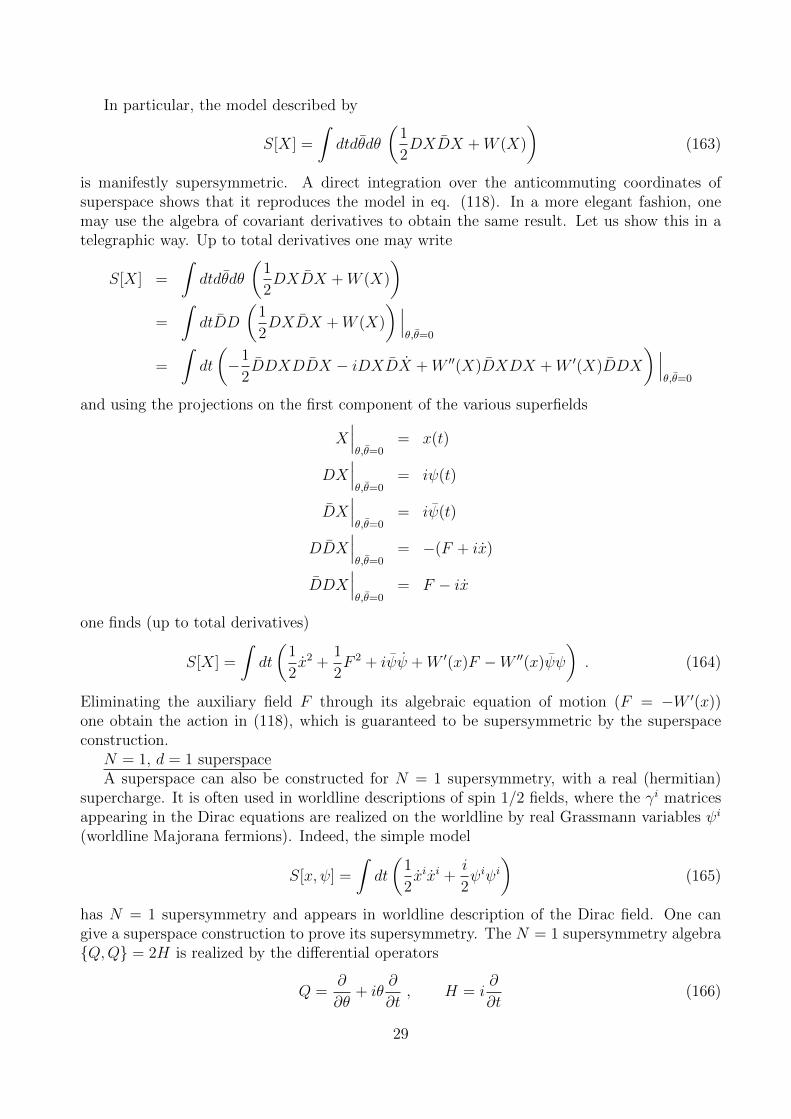
In particular, the model described by

S[X] =

∫dtdθdθ

(1

2DXDX +W (X)

)(163)

is manifestly supersymmetric. A direct integration over the anticommuting coordinates ofsuperspace shows that it reproduces the model in eq. (118). In a more elegant fashion, onemay use the algebra of covariant derivatives to obtain the same result. Let us show this in atelegraphic way. Up to total derivatives one may write

S[X] =

∫dtdθdθ

(1

2DXDX +W (X)

)=

∫dtDD

(1

2DXDX +W (X)

) ∣∣∣θ,θ=0

=

∫dt

(−1

2DDXDDX − iDXDX +W ′′(X)DXDX +W ′(X)DDX

) ∣∣∣θ,θ=0

and using the projections on the first component of the various superfields

X∣∣∣θ,θ=0

= x(t)

DX∣∣∣θ,θ=0

= iψ(t)

DX∣∣∣θ,θ=0

= iψ(t)

DDX∣∣∣θ,θ=0

= −(F + ix)

DDX∣∣∣θ,θ=0

= F − ix

one finds (up to total derivatives)

S[X] =

∫dt

(1

2x2 +

1

2F 2 + iψψ +W ′(x)F −W ′′(x)ψψ

). (164)

Eliminating the auxiliary field F through its algebraic equation of motion (F = −W ′(x))one obtain the action in (118), which is guaranteed to be supersymmetric by the superspaceconstruction.

N = 1, d = 1 superspaceA superspace can also be constructed for N = 1 supersymmetry, with a real (hermitian)

supercharge. It is often used in worldline descriptions of spin 1/2 fields, where the γi matricesappearing in the Dirac equations are realized on the worldline by real Grassmann variables ψi

(worldline Majorana fermions). Indeed, the simple model

S[x, ψ] =

∫dt

(1

2xixi +

i

2ψiψi

)(165)

has N = 1 supersymmetry and appears in worldline description of the Dirac field. One cangive a superspace construction to prove its supersymmetry. The N = 1 supersymmetry algebraQ,Q = 2H is realized by the differential operators

Q =∂

∂θ+ iθ

∂

∂t, H = i

∂

∂t(166)

29

that act on functions of superspace with coordinates (t, θ). The susy covariant derivative isgiven by

D =∂

∂θ− iθ ∂

∂t(167)

and anticommutes with Q. Using the superfields

X i(t, θ) = xi(t) + iθψi(t) (168)

one can construct in superspace the manifestly supersymmetric action

S[X] =i

2

∫dtdθDX iX i (169)

which reduces to (165) when passing to the superfield components.

30