bosons and fermions - fac.ksu.edu.sa

Perimeter Institute statistical physics Lecture Notes part 6: Bosons and fermions Version 1.5 9/11/09 Leo Kadanoff1

Bosons and fermionsSecond Quantization

Second Quantization vs ClassicalQuantum DescriptionOne Mode

Independent Excitations Extreme limit for fermions

Extreme limit for bosonsWaves

Waves= Special Bosonsphotons in cavitywaves as independent excitations

Conserved particlesconserved fermions in a boxconserved bosons in a boxbose transitiondynamics of fermions at low temperaturesLandau’s descriptiondynamics of bosons

Perimeter Institute statistical physics Lecture Notes part 6: Bosons and fermions Version 1.5 9/11/09 Leo Kadanoff

Second Quantized versus Classical Description

2

In a classical description, or even in using an ordinary wave function in a quantum description, we base everything on the particle. Particle 7 is sitting right in front of me; particle 23 is in the upper left hand corner, etc. A degenerate quantum system is one composed of identical particles sufficiently squeezed so that their wave functions overlap. To describe such a system, we cannot talk about the behavior of individual particles. We can only specify how many particles are doing this or that. Thus we start with a description of possible modes of the system and talk about their occupation. In this kind of description, we would say that there are seven particles in mode 3 and none in mode 2.

To discuss independent excitations in degenerate quantum theory, we use a formulation in which we allow the number of excitations to vary. Hence we are varying the number of particles. So instead of using exp(-βH), and keeping the number of particles fixed, we use as our weight function exp[-β(H-µN)] and we are allowing the number of particles to vary. The former approach is called using the canonical ensemble, and is what we have done up to now. The latter approach uses the grand canonical ensemble and it is the one we shall follow for this chapter.


Quantum Description

3

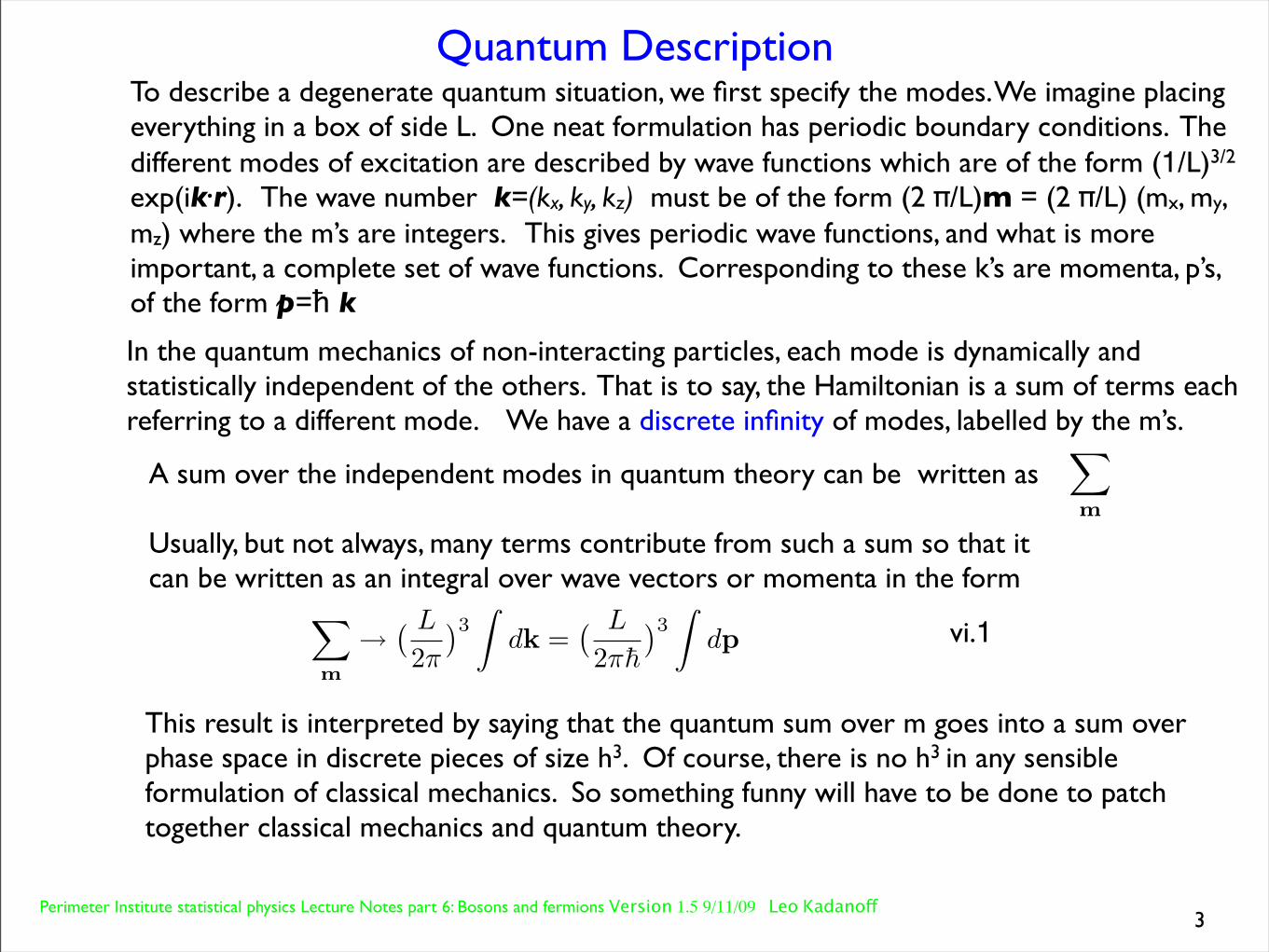
To describe a degenerate quantum situation, we first specify the modes. We imagine placing everything in a box of side L. One neat formulation has periodic boundary conditions. The different modes of excitation are described by wave functions which are of the form (1/L)3/2 exp(ik.r). The wave number k=(kx, ky, kz) must be of the form (2 π/L)m = (2 π/L) (mx, my, mz) where the m’s are integers. This gives periodic wave functions, and what is more important, a complete set of wave functions. Corresponding to these k’s are momenta, p’s, of the form p=ħ k

In the quantum mechanics of non-interacting particles, each mode is dynamically and statistically independent of the others. That is to say, the Hamiltonian is a sum of terms each referring to a different mode. We have a discrete infinity of modes, labelled by the m’s.

A sum over the independent modes in quantum theory can be written as

Usually, but not always, many terms contribute from such a sum so that it can be written as an integral over wave vectors or momenta in the form

∑

m

∑

m

→

( L

2π

)3

∫

dk =( L

2πh̄

)3

∫

dp

This result is interpreted by saying that the quantum sum over m goes into a sum over phase space in discrete pieces of size h3. Of course, there is no h3 in any sensible formulation of classical mechanics. So something funny will have to be done to patch together classical mechanics and quantum theory.

vi.1


One mode

4

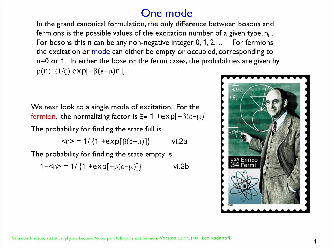
In the grand canonical formulation, the only difference between bosons and fermions is the possible values of the excitation number of a given type, nj . For bosons this n can be any non-negative integer 0, 1, 2, ... For fermions the excitation or mode can either be empty or occupied, corresponding to n=0 or 1. In either the bose or the fermi cases, the probabilities are given by ρ(n)=(1/ξ) exp[-β(ε-µ)n],

We next look to a single mode of excitation. For the fermion, the normalizing factor is ξ= 1 +exp[-β(ε-µ)]

The probability for finding the state full is

<n> = 1/ {1 +exp[β(ε-µ)]} vi.2aThe probability for finding the state empty is

1-<n> = 1/ {1 +exp[-β(ε-µ)]} vi.2b


Extreme Limits for fermions

5

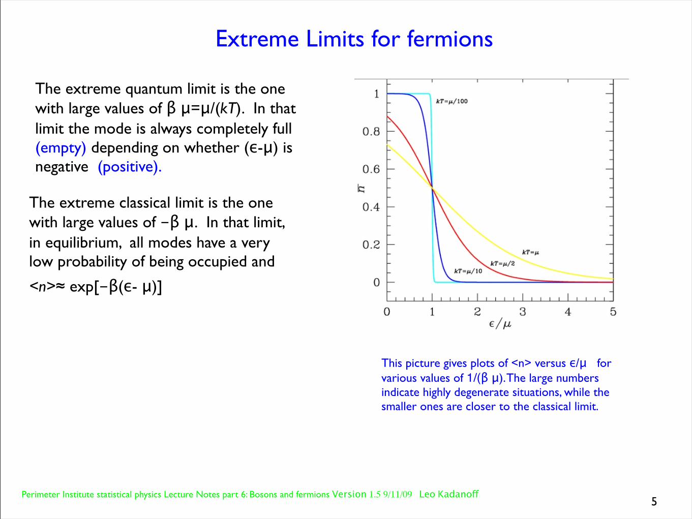
The extreme quantum limit is the one with large values of β μ=μ/(kT). In that limit the mode is always completely full (empty) depending on whether (ε-μ) is negative (positive).

The extreme classical limit is the one with large values of -β μ. In that limit, in equilibrium, all modes have a very low probability of being occupied and

<n>≈ exp[-β(ε- μ)]

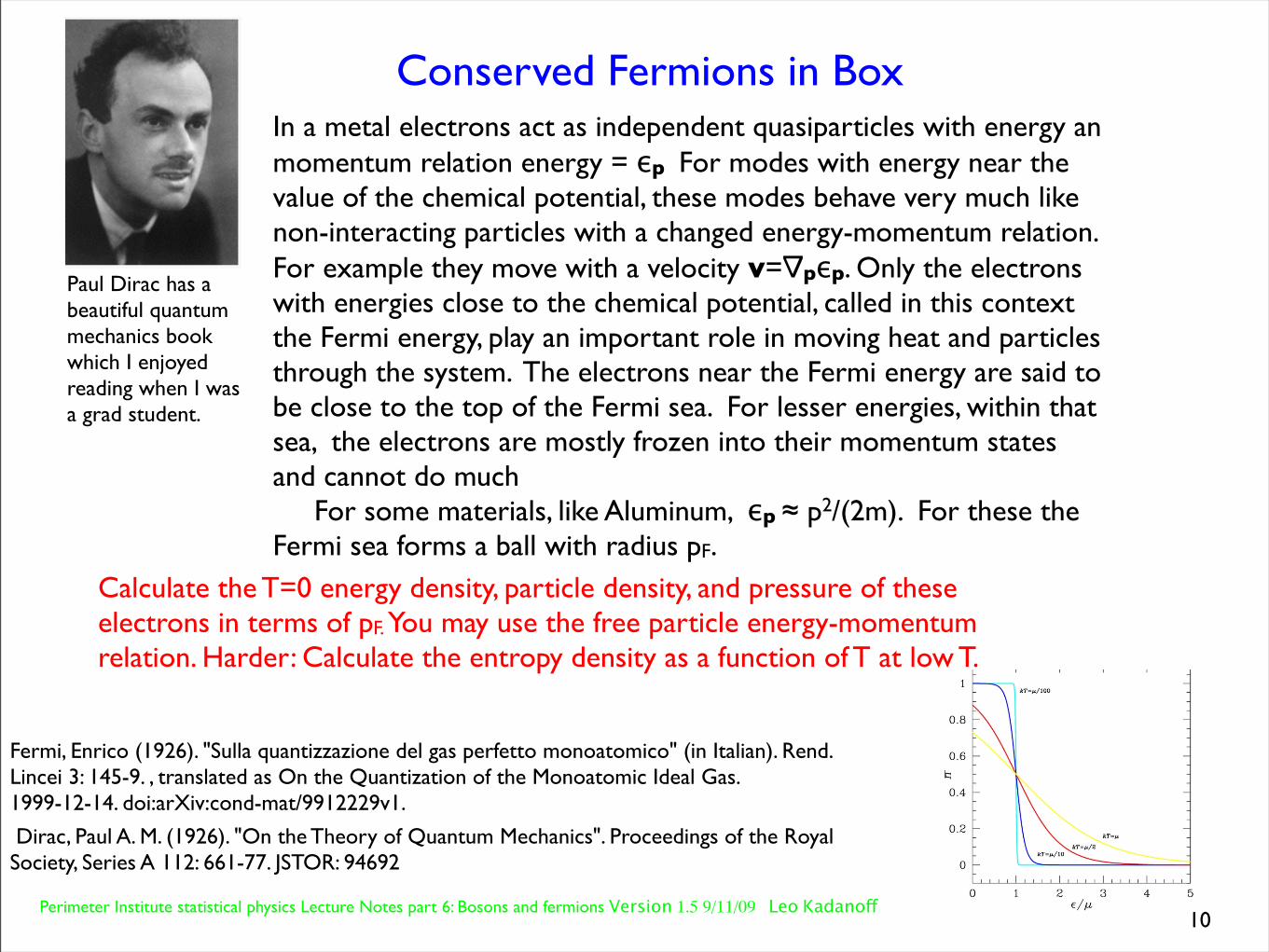
This picture gives plots of <n> versus ε/μ for various values of 1/(β μ). The large numbers indicate highly degenerate situations, while the smaller ones are closer to the classical limit.


the equilibrium probability distribution for occupation of the single mode is ρ(n)=(1/ξ) exp[-β(ε-µ)n]. All integer values of n between zero and infinity are permitted.

The normalizing factor is

ξ= 1 +exp[-β(ε-µ)] + +exp[-2β(ε-µ)]+ +exp[-3β(ε-µ)] +...

ξ=1/{1 -exp[-β(ε-µ)]}

Note that ε-µ must be positive.

The average occupation is <n> = 1/ {exp[β(ε-µ)]-1} vi.3An extreme quantum limit is the one with very small positive values of β (ε-µ). In that limit, the mode can have lots and lots of quanta in it. You can even have macroscopic occupation of a single mode, in which a finite fraction of the entire number of particles is in a single mode. This is also called Bose-Einstein condensation after the discoverers of this effect.

For the boson

Satyendra Nath Bose

The extreme classical limit is once more a very large value of -β μ and a small average occupation of the state. Once more <n>≈ exp[-β(ε- μ)] in this limit.Bosons need not be conserved. If they are not conserved, the equilibrium situation has μ=0.


Independent Excitations: waves

7

One example of a boson excitation is provided by a set of waves. There are two major examples: light waves and sound waves. In these two cases, the quanta are called respectively photons and phonons. In the simplest situation, the Hamiltonian for the system is a sum over terms corresponding to the different excitations in the system

Here, εj is the energy of a single excitation of type j and nj is the number of excitations of that type. These quanta have the property that they are not conserved. When the basic objects under consideration are conserved quantities, e.g. atoms or molecules, and they don’t interact, the Hamiltonian is of exactly the same form, but it is convenient to use a statistical theory in which we allow the total number of particles to vary, and use a probability function of the form

H =

∑

j

εjnj vi.4

and the statistical mechanics is given by the usual formula ρ{n}=(1/Ξ) exp(-βH{n}) where the normalizer, Ξ, is called the grand partition function.

ρ{n}=(1/Ξ) exp(-β[H{n}-μN{n}]) where N is the total particle number

N =

∑

j

nj

Here µ is called the chemical potential. The density of particles increases as µ increases.


Waves=Special bosons

8

ε=ħω, so in the classical limit the energy of a photon goes to zero.

the probability distribution for the single mode is

ρ(n)=(1/ξ) exp[-β ε n]

The normalizing factor is

ξ= 1 +exp[-β ε] + +exp[-2β ε]+ +exp[-3β ε] +... so that

Note that ε must be positive or zero. The average energy in the mode is <n>ε = ε/ {exp[β ε]-1}= ħω/ {exp[β ħω]-1}

Classical limit = high temperature <n>ε=1/ β = kT

Therefore classical physics gives kT per mode. A cavity has an infinite number of electromagnetic modes. Therefore, a cavity has infinite energy?!?

In quantum theory high frequency modes are cut off because they must have small average occupations numbers, <n>. Therefore the classical result of kT per mode is simply wrong. So there is no infinity.

In this way, Planck helped us get the right answer by introducing photons and starting off the talk about occupation numbers!

ξ= ___________11 -exp[-β ε]


photons in Cubic Cavity

9

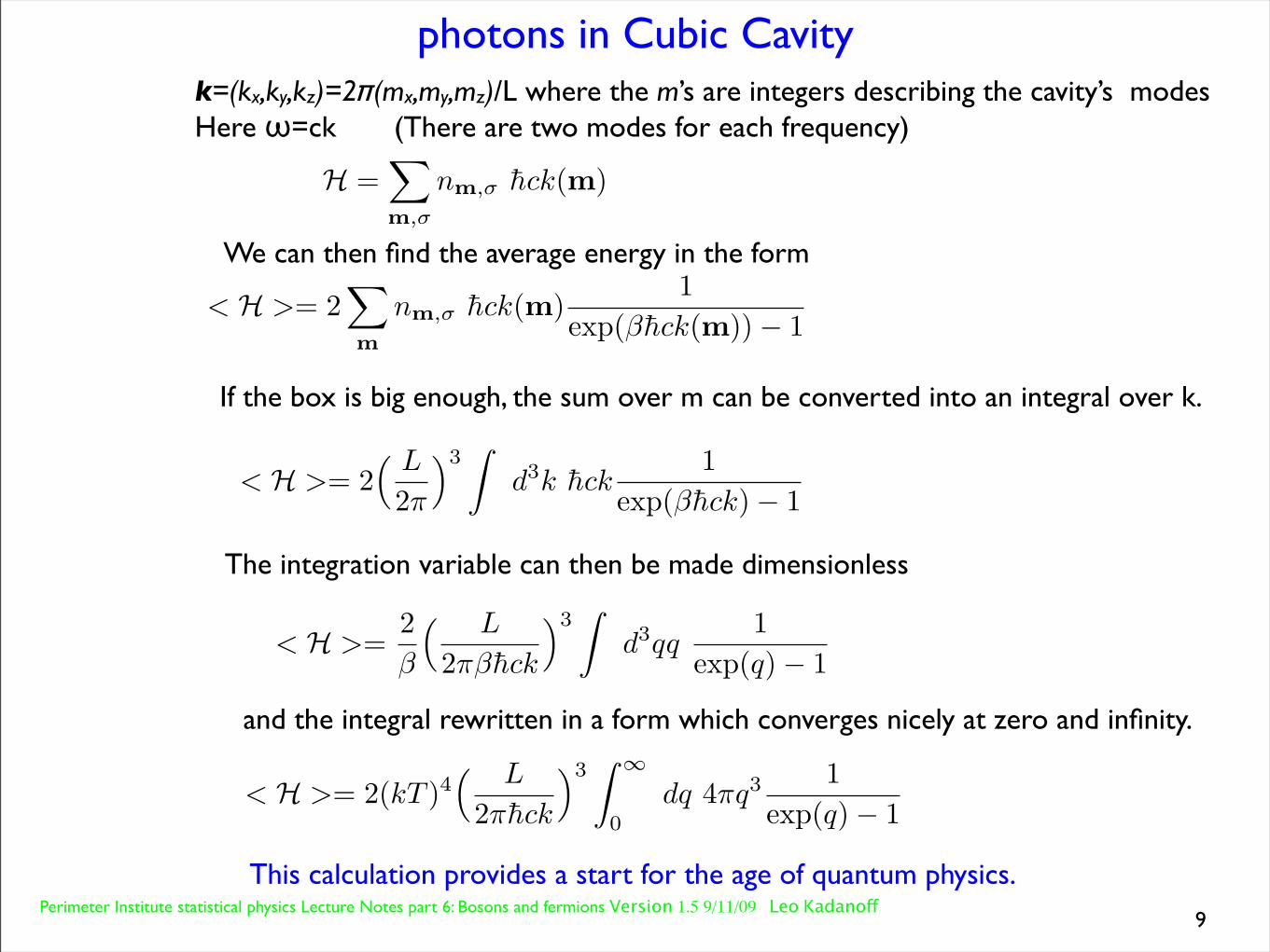
k=(kx,ky,kz)=2π(mx,my,mz)/L where the m’s are integers describing the cavity’s modes Here ω=ck (There are two modes for each frequency)

H =∑

m,σ

nm,σ h̄ck(m)

< H >= 2∑

m

nm,σ h̄ck(m)1

exp(βh̄ck(m)) − 1

We can then find the average energy in the form

If the box is big enough, the sum over m can be converted into an integral over k.

< H >= 2( L

2π

)3∫

d3k h̄ck1

exp(βh̄ck) − 1

The integration variable can then be made dimensionless

< H >=2

β

( L

2πβh̄ck

)3∫

d3qq1

exp(q) − 1

< H >= 2(kT )4( L

2πh̄ck

)3∫

∞

0

dq 4πq3 1

exp(q) − 1

and the integral rewritten in a form which converges nicely at zero and infinity.

This calculation provides a start for the age of quantum physics.


Conserved Fermions in Box

10

Fermi, Enrico (1926). "Sulla quantizzazione del gas perfetto monoatomico" (in Italian). Rend. Lincei 3: 145-9. , translated as On the Quantization of the Monoatomic Ideal Gas. 1999-12-14. doi:arXiv:cond-mat/9912229v1.

Dirac, Paul A. M. (1926). "On the Theory of Quantum Mechanics". Proceedings of the Royal Society, Series A 112: 661-77. JSTOR: 94692

Paul Dirac has a beautiful quantum mechanics book which I enjoyed reading when I was a grad student.

In a metal electrons act as independent quasiparticles with energy an momentum relation energy = εp For modes with energy near the value of the chemical potential, these modes behave very much like non-interacting particles with a changed energy-momentum relation. For example they move with a velocity v=∇pεp. Only the electrons with energies close to the chemical potential, called in this context the Fermi energy, play an important role in moving heat and particles through the system. The electrons near the Fermi energy are said to be close to the top of the Fermi sea. For lesser energies, within that sea, the electrons are mostly frozen into their momentum states and cannot do much For some materials, like Aluminum, εp ≈ p2/(2m). For these the Fermi sea forms a ball with radius pF.

Calculate the T=0 energy density, particle density, and pressure of these electrons in terms of pF. You may use the free particle energy-momentum relation. Harder: Calculate the entropy density as a function of T at low T.


Conserved Bosons in Box

11

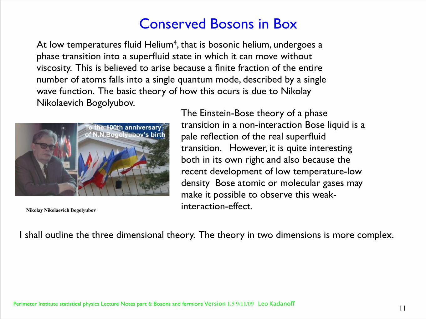
At low temperatures fluid Helium4, that is bosonic helium, undergoes a phase transition into a superfluid state in which it can move without viscosity. This is believed to arise because a finite fraction of the entire number of atoms falls into a single quantum mode, described by a single wave function. The basic theory of how this ocurs is due to Nikolay Nikolaevich Bogolyubov.

Nikolay Nikolaevich Bogolyubov

The Einstein-Bose theory of a phase transition in a non-interaction Bose liquid is a pale reflection of the real superfluid transition. However, it is quite interesting both in its own right and also because the recent development of low temperature-low density Bose atomic or molecular gases may make it possible to observe this weak-interaction-effect.

I shall outline the three dimensional theory. The theory in two dimensions is more complex.


Bose Transition

12

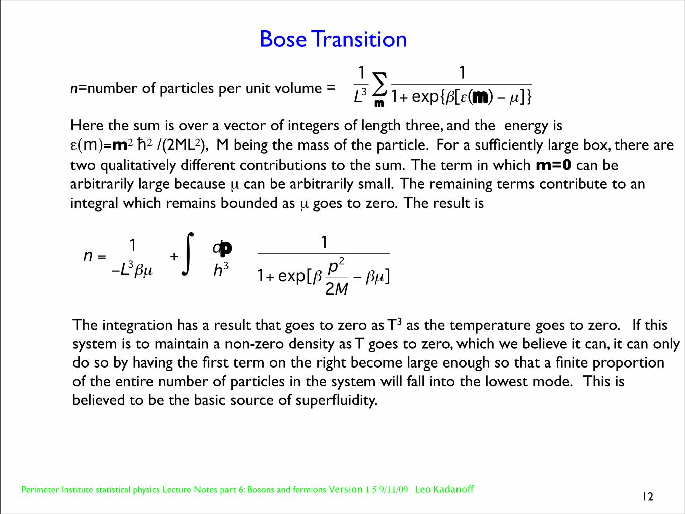
The integration has a result that goes to zero as T3 as the temperature goes to zero. If this system is to maintain a non-zero density as T goes to zero, which we believe it can, it can only do so by having the first term on the right become large enough so that a finite proportion of the entire number of particles in the system will fall into the lowest mode. This is believed to be the basic source of superfluidity.

∫

€

n =1

−L3βµ+∫

€

1

1+ exp[β p2

2M− βµ]

€

dph3

n=number of particles per unit volume =

Here the sum is over a vector of integers of length three, and the energy is ε(m)=m2 ħ2 /(2ML2), M being the mass of the particle. For a sufficiently large box, there are two qualitatively different contributions to the sum. The term in which m=0 can be arbitrarily large because µ can be arbitrarily small. The remaining terms contribute to an integral which remains bounded as µ goes to zero. The result is

€

1L3

11+ exp{β[ε(m) − µ]}m

∑


Dynamics of fermions at low temperature

13

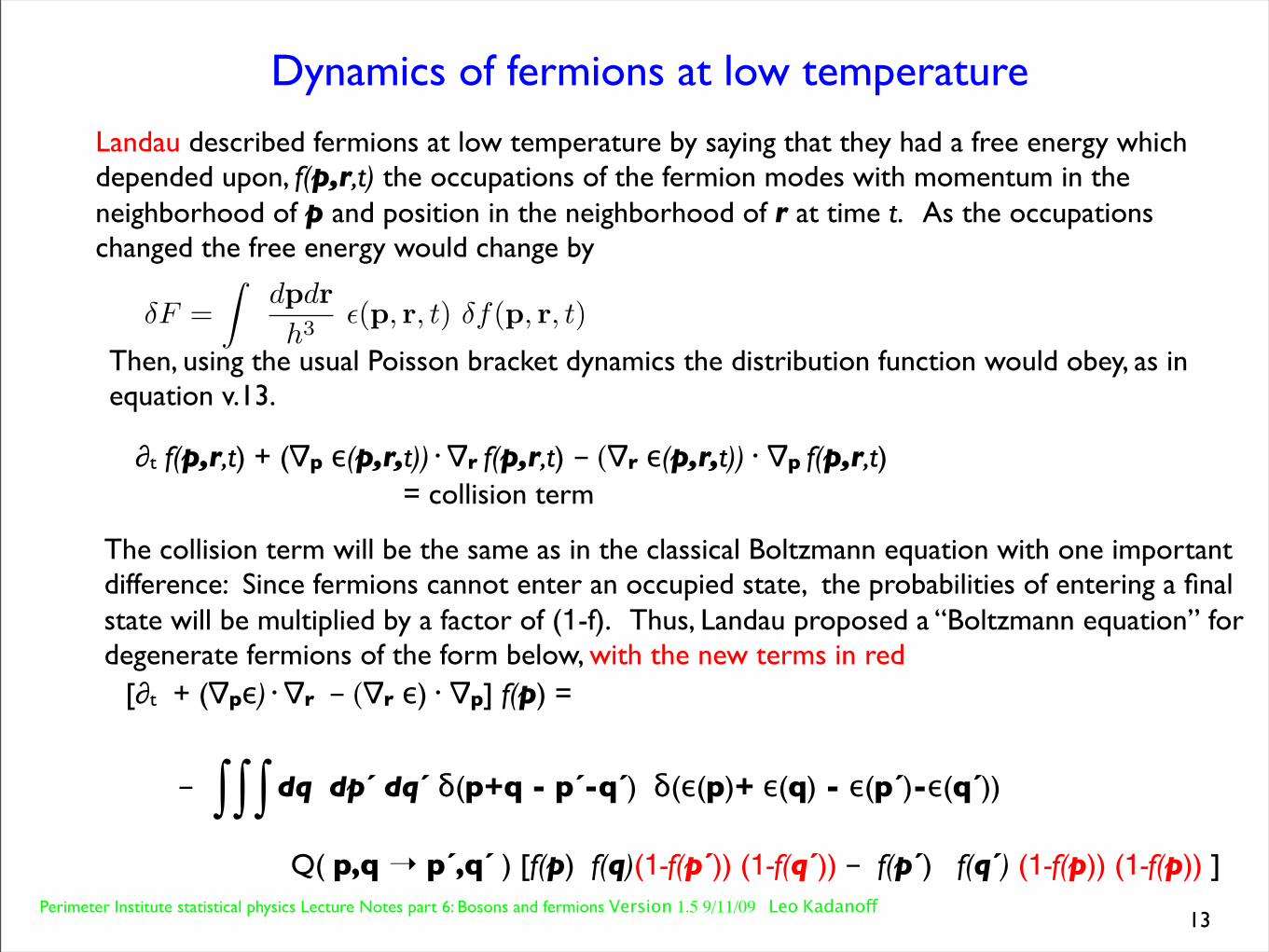
Landau described fermions at low temperature by saying that they had a free energy which depended upon, f(p,r,t) the occupations of the fermion modes with momentum in the neighborhood of p and position in the neighborhood of r at time t. As the occupations changed the free energy would change by

1234567890-=θωερτψυιοπ[]∴ασδφγηϕκλ;∏ζξχϖβνμ,./

δF =

∫dpdr

h3ε(p, r, t) δf(p, r, t)

Then, using the usual Poisson bracket dynamics the distribution function would obey, as in equation v.13.

∂t f(p,r,t) + (∇p ε(p,r,t)) . ∇r f(p,r,t) - (∇r ε(p,r,t)) . ∇p f(p,r,t)= collision term

The collision term will be the same as in the classical Boltzmann equation with one important difference: Since fermions cannot enter an occupied state, the probabilities of entering a final state will be multiplied by a factor of (1-f). Thus, Landau proposed a “Boltzmann equation” for degenerate fermions of the form below, with the new terms in red

[∂t + (∇pε) . ∇r - (∇r ε) . ∇p] f(p) =

- dq dp´ dq´ δ(p+q - p´-q´) δ(ε(p)+ ε(q) - ε(p´)-ε(q´))

Q( p,q ➝ p´,q´ ) [f(p) f(q)(1-f(p´)) (1-f(q´)) - f(p´) f(q´) (1-f(p)) (1-f(p)) ]

∫∫∫


Landau’s equation for low temperature fermion systems:

14

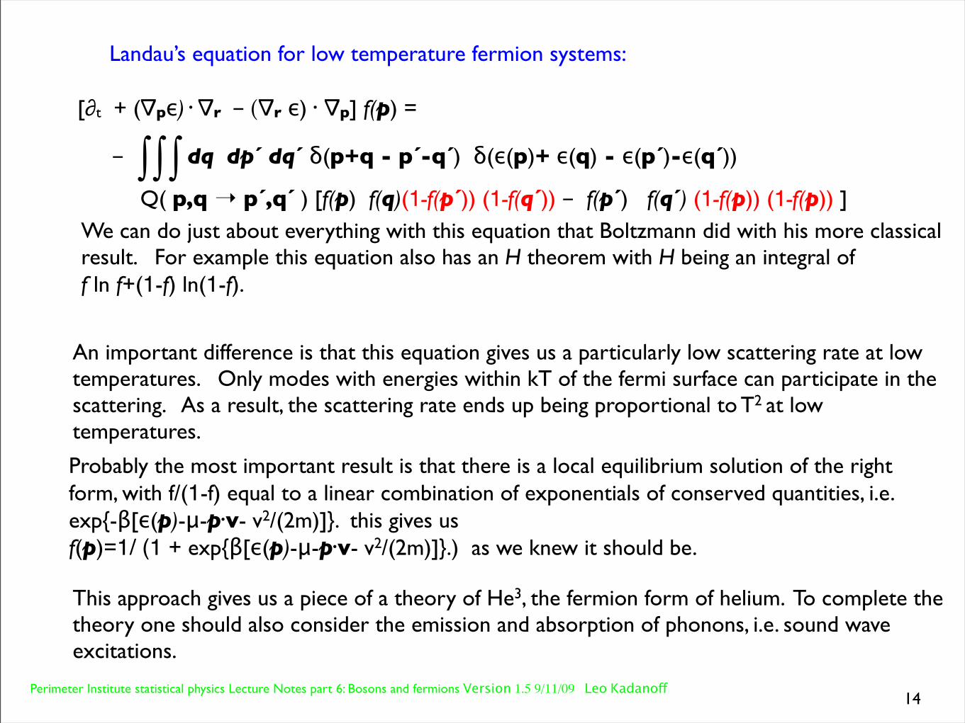
[∂t + (∇pε) . ∇r - (∇r ε) . ∇p] f(p) =


Q( p,q ➝ p´,q´ ) [f(p) f(q)(1-f(p´)) (1-f(q´)) - f(p´) f(q´) (1-f(p)) (1-f(p)) ]∫∫∫

We can do just about everything with this equation that Boltzmann did with his more classical result. For example this equation also has an H theorem with H being an integral of f ln f+(1-f) ln(1-f).

An important difference is that this equation gives us a particularly low scattering rate at low temperatures. Only modes with energies within kT of the fermi surface can participate in the scattering. As a result, the scattering rate ends up being proportional to T2 at low temperatures.

Probably the most important result is that there is a local equilibrium solution of the right form, with f/(1-f) equal to a linear combination of exponentials of conserved quantities, i.e.exp{-β[ε(p)-μ-p.v- v2/(2m)]}. this gives us f(p)=1/ (1 + exp{β[ε(p)-μ-p.v- v2/(2m)]}.) as we knew it should be.

This approach gives us a piece of a theory of He3, the fermion form of helium. To complete the theory one should also consider the emission and absorption of phonons, i.e. sound wave excitations.


Dynamics of bosons

15

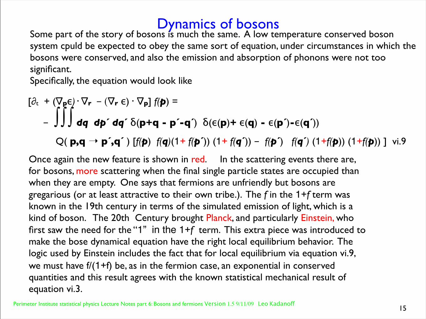
Some part of the story of bosons is much the same. A low temperature conserved boson system cpuld be expected to obey the same sort of equation, under circumstances in which the bosons were conserved, and also the emission and absorption of phonons were not too significant.Specifically, the equation would look like

[∂t + (∇pε) . ∇r - (∇r ε) . ∇p] f(p) =


Q( p,q ➝ p´,q´ ) [f(p) f(q)(1+ f(p´)) (1+ f(q´)) - f(p´) f(q´) (1+f(p)) (1+f(p)) ] vi.9

∫∫∫

Once again the new feature is shown in red. In the scattering events there are, for bosons, more scattering when the final single particle states are occupied than when they are empty. One says that fermions are unfriendly but bosons are gregarious (or at least attractive to their own tribe.). The f in the 1+f term was known in the 19th century in terms of the simulated emission of light, which is a kind of boson. The 20th Century brought Planck, and particularly Einstein, who first saw the need for the “1” in the 1+f term. This extra piece was introduced to make the bose dynamical equation have the right local equilibrium behavior. The logic used by Einstein includes the fact that for local equilibrium via equation vi.9, we must have f/(1+f) be, as in the fermion case, an exponential in conserved quantities and this result agrees with the known statistical mechanical result of equation vi.3.


References

16

Daniel Kleppner., “Rereading Einstein on Radiation”, Physics Today, (February 2005).

A Einstein, Phys. Z. 18 121 (1917). English translation, D. ter Haar, The Old Quantum Theory, Pergamon Press, New York, p. 167 (1967).

bosons and fermions - fac.ksu.edu.sa

Documents