Passive microwave measurements of sea ice

Leif Toudal Pedersen, DMI

Natalia Ivanova, NERSC

Thomas Lavergne, met.no

Rasmus Tonboe, DMI

Roberto Saldo, DTU

Marko Mäkynen, FMI

Georg Heygster, U-Bremen

Anja Rösel, U-Hamburg

Stefan Kern, U-Hamburg

Gorm Dybkjær, DMI

Algorithm evaluation

• Sensitivity to atmosphere

– Open water dataset

– Simulated data incl RTM corrected TBs from RRDP

– Met/ocean data screening

• Sensitivity to emissivity variations

– 100% ice dataset

– Simulated data

– Snow/ice/atmosphere data screening

• Summer performance (snow/ice melt and melt-ponds)

• SMMR vs SSMI vs AMSR-E performance

• Thin ice performance

• Potential resolution

Convergence at ca. 100%

• Deformation field between 20100109 and 20100110 from ENVISAT ASAR WSM

Dataset of daily data from June 2007to present exists from PolarView/MyOcean at DTU

Red: ConvergenceBlue: Divergence

Distribution of validation data (2008 example)

Algorithm portefolio

• Some new algorithms (combinations) were added

Main results for SIC0 and SIC1

No WF!

Workings of N90 algorithms

Artificial data combinations

• Some algorithms have cut-offs/non-linearities that does not allow a thorough validation at only 0 and 100% ice.

• We have generated a dataset of 15% ice and 85% ice using our 0% and 100%

• SIC15 = 0.85*SIC0(t)+0.15*SIC100(avgFY)

• SIC85 = 0.85*SIC100(t)+0.15*SIC0(avgW)

Algorithm comparison, SIC=15%, AMSR, no WF

Near 9

0GHz

Near 9

0GHz

lin, d

yn ASIP90

(NRL+N90

Lin)/2

(CF+N90

L)/2

(NRL+CF+N90

Lin)/3

Bootstra

p P (C

P)P37

(NT+CF+N90

Lin)/3

ECICE

P18 PR

Bristo

l

NASA Tea

m 2

(CF+N90

L*CF)/(

1+CF)

NASA Tea

m (N

T)

OSIS

AF-2

OSIS

AF

(NT+CF)/2 P10

(CF+N90

L*CF**

2)/(1

+CF**2)

(CF+N90

L*CF**

3)/(1

+CF**3)

OSIS

AF-3

UMas

s-AES

TUD

NORSEX

CalVal

Bootstra

p F (C

F)

One

chan

nel (6

H)

IOM

ASA IRT

0

5

10

15

20

25

30

35

Algorithm comparison, SIC=85%

PRP18 P37 P10

Bootstra

p P

(NRL+N90

Lin)/2 P90

Near 9

0GHz

lin, d

yn

IOM

ASA IRT

Bootstra

p F

CalVal

UMas

s-AES

TUD

NORSEX

Near 9

0GHz

NASA Tea

m

One

chan

nel (6

H)ASI

(NRL+CF+N90

Lin)/3

ECICE

(CF+N90

L*CF**

3)/(1

+CF**3)

(CF+N90

L)/2

(CF+N90

L*CF**

2)/(1

+CF**2)

(CF+N90

L*CF)/(

1+CF)

(NT+CF+N90

Lin)/3

Bristo

l

OSIS

AF

OSIS

AF-2

OSIS

AF-3

(NT+CF)/2

NASA Tea

m 2

0

5

10

15

20

25

30

35

NT2

• Has a bias of 10-15% at 85% ice, so a lot of datapoints at 85% are truncated at 100%

• Real performance at SIC=85% is something like 10% (estimated from SSMI results that are less biased)

AMSR Summer SIC=0

Weather filters

• Weather filters are supposed to remove open water points that show ice because of atmospheric influence (set SIC=0) .

• We have established further artificial datasets at 20, 25 and 30% SIC for testing of weather filters.

Weather filters

ICE

ICE

ICE

ICE

Weather filters

• Tested and we found that they remove ice up to sic>25%

• We therefore generated a subset of RRDP with appended ERA Interim– Calculated corrections of TBs due to wind,

water vapour and temp. Tried CLW but it was bad

• Applied all algorithms to this new set

Atmospheric correction

Upwelling + surface contrib.

Reflected downwelling contrib.

Reflected sky contrib.

Tap = εTs + n

Atmospheric correction

Stdev at SIC=0before and after Atm correction

Still no WF

Atmospheric correction using RTM

• CF algorithm before and after RTM correction with ERA INTERIM

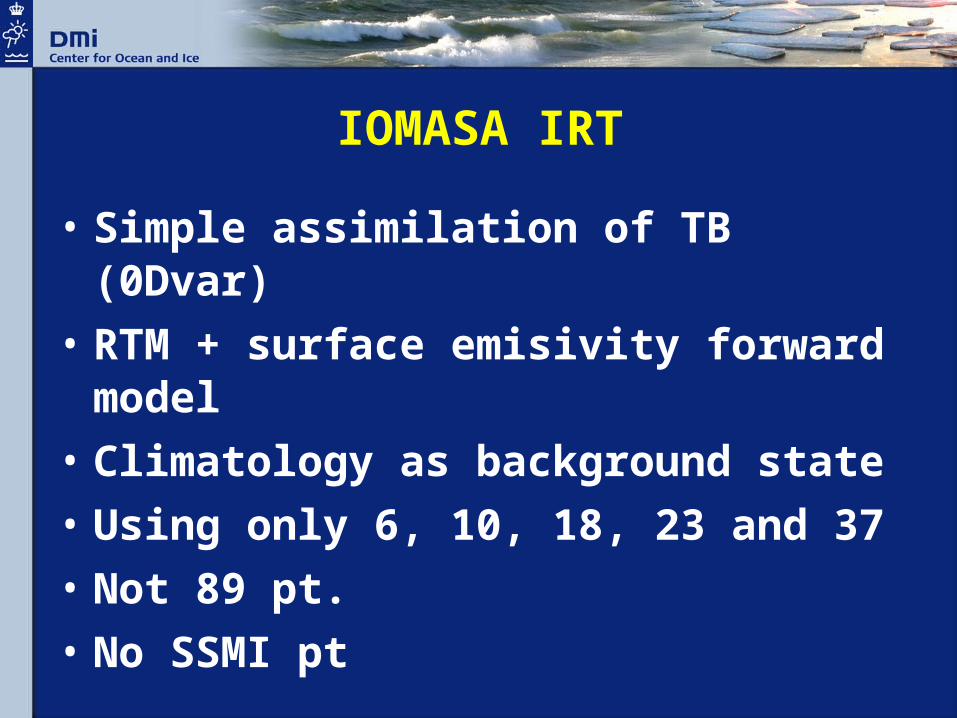
IOMASA IRT

• Simple assimilation of TB (0Dvar)

• RTM + surface emisivity forward model

• Climatology as background state

• Using only 6, 10, 18, 23 and 37

• Not 89 pt.

• No SSMI pt

AMSR - February 4, 2006

Ice concentration MY-fraction Ice temperature ”Error”

SSTWater Vapour Cloud liquid water Wind Speed

RRDP results, SIC=0

• Small RMS error

• 1.71%

• Small bias

• -0.05%

-8 -7 -6 -5 -4 -3 -2 -1 0 1 2 3 4 5 6 7 80

1000

2000

3000

4000

5000

6000

7000

Integrated retrieval of SIC=0, all year

Frequency

CF(rtm) vs IOMASA(irt) for SIC=0

0,0

50,0

100,0

150,0

200,0

-10,0 -5,0 0,0 5,0 10,0

Histogram

Bootstrap_f

Co

un

t

0,0

500,0

1000,0

1500,0

2000,0

-0,1 -0,1 0,0 0,1 0,1

Histogram

SICx

Co

un

t

Stdev=2.50 (before atm 4.3) Stdev=1.71

Ice conc in fractions of 1Ice conc in %

Algorithm comparison, SIC=15%, AMSR, no WF

Near 9

0GHz

Near 9

0GHz

lin, d

yn ASIP90

(NRL+N90

Lin)/2

(CF+N90

L)/2

(NRL+CF+N90

Lin)/3

Bootstra

p P (C

P)P37

(NT+CF+N90

Lin)/3

ECICE

P18 PR

Bristo

l

NASA Tea

m 2

(CF+N90

L*CF)/(

1+CF)

NASA Tea

m (N

T)

OSIS

AF-2

OSIS

AF

(NT+CF)/2 P10

(CF+N90

L*CF**

2)/(1

+CF**2)

(CF+N90

L*CF**

3)/(1

+CF**3)

OSIS

AF-3

UMas

s-AES

TUD

NORSEX

CalVal

Bootstra

p F (C

F)

One

chan

nel (6

H)

IOM

ASA IRT

0

5

10

15

20

25

30

35

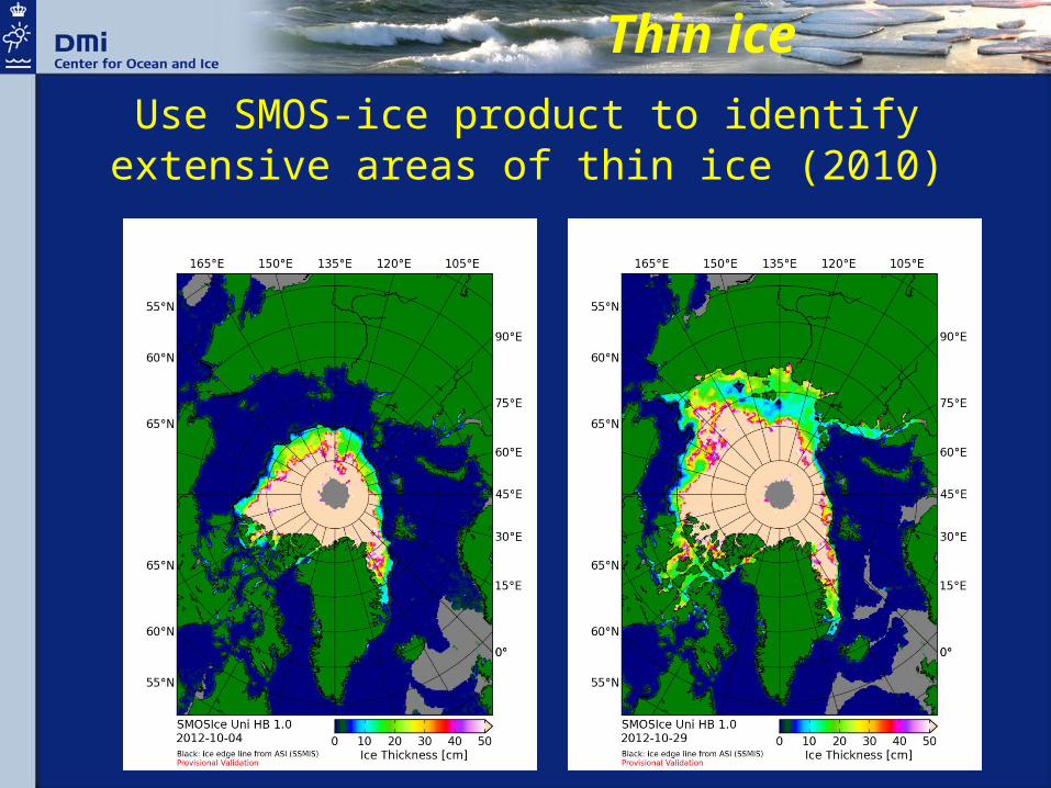
Use SMOS-ice product to identify extensive areas of thin ice (2010)

Thin ice

0.04

0.05

0.06

0.07

0.08

0.09 0.1

0.11

0.12

0.13

0.14

0.15

0.16

0.17

0.18

0.19 0.2

0.21

0.22

0.23

0.24

0.25

0.26

0.27

0.28

0.29

0.0

0.2

0.4

0.6

0.8

1.0

1.2

ASI

CF

Bristol

NT

NT2

N90

NORSEX

6H

TUD

AES

SIC(SMOS Ice Thickness)

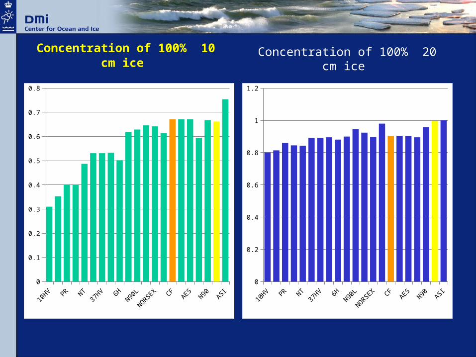
Concentration of 100% 10 cm ice

10HV PR NT

37HV 6H

N90L

NORSEX CFAES

N90 ASI0

0.1

0.2

0.3

0.4

0.5

0.6

0.7

0.8

10HV PR NT

37HV 6H

N90L

NORSEX CFAES

N90 ASI0

0.2

0.4

0.6

0.8

1

1.2

Concentration of 100% 20 cm ice

Melt pond dataset distribution

SIC vs (1-OW)OW is melt ponds + leads

Combination of melted snow/ice that causes overestimation and OW that does the opposite

Data format for validation dataSimple comma separated ASCII text file

(.csv)

Conclusions

• We select a relatively simple and linear algorithm (CF or OSISAF)

• We perform atmospheric correction to TBs to reduce atm noise

• We apply dynamic tie-points to accomodate residual sensor drift and seasonal cycle in signatures

The end

Thank you for your attention