parties, models, mobsters - uibk.ac.atzeileis/papers/psychoco-2014.pdf · overview model-based...
TRANSCRIPT

Parties, Models, MobstersA New Implementation of Model-Based Recursive Partitioning in R
Achim Zeileis, Torsten Hothorn
http://eeecon.uibk.ac.at/~zeileis/

Overview
Model-based recursive partitioningA generic approachExample: Bradley-Terry trees
Implementation in RBuilding blocks: Parties, models, mobstersOld implementation in partyAll new implementation in partykit
Illustration

Model-based recursive partitioning
Models: Estimation of parametric models with observations yi (andregressors xi ), parameter vector θ, and additive objective function Ψ.
θ̂ = argminθ
∑i
Ψ(yi , xi , θ).
Recursive partitioning:
1 Fit the model in the current subsample.2 Assess the stability of θ across each partitioning variable zj .3 Split sample along the zj∗ with strongest association: Choose
breakpoint with highest improvement of the model fit.4 Repeat steps 1–3 recursively in the subsamples until some
stopping criterion is met.
Model-based recursive partitioning
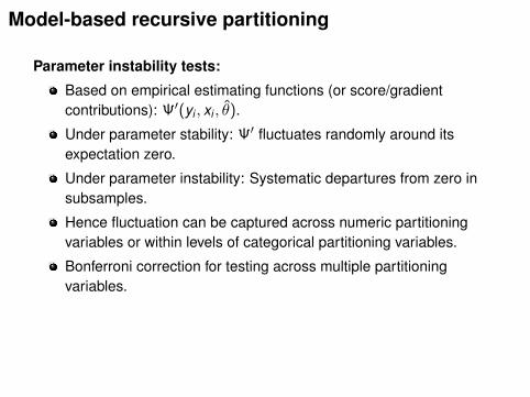
Parameter instability tests:
Based on empirical estimating functions (or score/gradientcontributions): Ψ′(yi , xi , θ̂).
Under parameter stability: Ψ′ fluctuates randomly around itsexpectation zero.
Under parameter instability: Systematic departures from zero insubsamples.
Hence fluctuation can be captured across numeric partitioningvariables or within levels of categorical partitioning variables.
Bonferroni correction for testing across multiple partitioningvariables.

Bradley-Terry trees
Questions: Which of thesewomen is more attractive?How does the answer depend onage, gender, and the familiaritywith the associated TV showGermany’s Next Topmodel?

Bradley-Terry trees
agep < 0.001
1
≤ 52 > 52
q2p = 0.017
2
yes no
Node 3 (n = 35)
●●
●
●●
●
B Ann H F M Anj
0
0.5
genderp = 0.007
4
male female
Node 5 (n = 71)
●
●
●
●
● ●
B Ann H F M Anj
0
0.5Node 6 (n = 56)
●
●
●
●
●
●
B Ann H F M Anj
0
0.5Node 7 (n = 30)
●
●
● ● ●
●
B Ann H F M Anj
0
0.5
Implementation: Building blocks
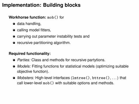
Workhorse function: mob() for
data handling,
calling model fitters,
carrying out parameter instability tests and
recursive partitioning algorithm.
Required functionality:
Parties: Class and methods for recursive partytions.
Models: Fitting functions for statistical models (optimizing suitableobjective function).
Mobsters: High-level interfaces (lmtree(), bttree(), . . . ) thatcall lower-level mob() with suitable options and methods.

Implementation: Old mob() in party
Parties: S4 class ‘BinaryTree’.
Originally developed only for ctree() and somewhat “abused”.
Rather rigid and hard to extend.
Models: S4 ‘StatModel’ objects.
Intended to conceptualize unfitted model objects.
Required some “glue code” to accomodate non-standard interfacefor data handling and model fitting.
Mobsters:
mob() already geared towards (generalized) linear models.
Other interfaces in psychotree and betareg.
Hard to do fine control due to adopted S4 classes: Manyunnecessary computations and copies of data.

Implementation: New mob() in partykit
Parties: S3 class ‘modelparty’ built on ‘party’.
Separates data and tree structure.
Inherits generic infrastructure for printing, predicting, plotting, . . .
Models: Plain functions with input/output convention.
Basic and extended interface for rapid prototyping and forspeeding up computings, respectively.
Only minimial glue code required if models are well-designed.
Mobsters:
mob() completely agnostic regarding models employed.
Separate interfaces lmtree(), glmtree(), . . .
New interfaces typically need to bring their model fitter and adaptthe main methods print(), plot(), predict() etc.

Implementation: New mob() in partykit
New inference options: Not used by default by optionally available.
New parameter instability tests for ordinal partitioning variables.Alternative to unordered χ2 test but computationally intensive.
Post-pruning based on information criteria (e.g., AIC or BIC),especially for very large datasets where traditional significancelevels are not useful.
Multiway splits for categorical partitioning variables.
Treat weights as proportionality weights and not as case weights.

Implementation: Models
Input: Basic interface.
fit(y, x = NULL, start = NULL, weights = NULL,
offset = NULL, ...)
y, x, weights, offset are (the subset of) the preprocessed data.Starting values and further fitting arguments are in start and ....
Output: Fitted model object of class with suitable methods.
coef(): Estimated parameters θ̂.
logLik(): Maximized log-likelihood function −∑
i Ψ(yi , x,θ̂).
estfun(): Empirical estimating functions Ψ′(yi , xi , θ̂).

Implementation: Models
Input: Extended interface.
fit(y, x = NULL, start = NULL, weights = NULL,
offset = NULL, ..., estfun = FALSE, object = FALSE)
Output: List.
coefficients: Estimated parameters θ̂.
objfun: Minimized objective function∑
i Ψ(yi , x,θ̂).
estfun: Empirical estimating functions Ψ′(yi , xi , θ̂). Only neededif estfun = TRUE, otherwise optionally NULL.
object: A model object for which further methods could beavailable (e.g., predict(), or fitted(), etc.). Only needed ifobject = TRUE, otherwise optionally NULL.
Internally: Extended interface constructed from basic interface ifsupplied. Efficiency can be gained through extended approach.

Illustration: Bradley-Terry trees
Data, packages, and estfun() method:R> data("Topmodel2007", package = "psychotree")R> library("partykit")R> library("psychotools")R> estfun.btReg <- function(x, ...) x$estfun
Basic model fitting function:
R> btfit1 <- function(y, x = NULL, start = NULL, weights = NULL,+ offset = NULL, ...) btReg.fit(y, weights = weights, ...)
Fit Bradley-Terry tree:
R> system.time(bt1 <- mob(+ preference ~ 1 | gender + age + q1 + q2 + q3,+ data = Topmodel2007, fit = btfit1))
user system elapsed5.112 0.020 5.263

Illustration: Bradley-Terry trees
Extended model fitting function:
R> btfit2 <- function(y, x = NULL, start = NULL, weights = NULL,+ offset = NULL, ..., estfun = FALSE, object = FALSE) {+ rval <- btReg.fit(y, weights = weights, ...,+ estfun = estfun, vcov = object)+ list(+ coefficients = rval$coefficients,+ objfun = -rval$loglik,+ estfun = if(estfun) rval$estfun else NULL,+ object = if(object) rval else NULL+ )+ }
Fit Bradley-Terry tree again:
R> system.time(bt2 <- mob(+ preference ~ 1 | gender + age + q1 + q2 + q3,+ data = Topmodel2007, fit = btfit2))
user system elapsed4.004 0.012 4.087

Illustration: Bradley-Terry trees
Model-based recursive partitioning (btfit2)
Model formula:preference ~ 1 | gender + age + q1 + q2 + q3
Fitted party:[1] root| [2] age <= 52| | [3] q2 in yes: n = 35| | Barbara Anni Hana Fiona Mandy| | 1.3378 1.2318 2.0499 0.8339 0.6217| | [4] q2 in no| | | [5] gender in male: n = 71| | | Barbara Anni Hana Fiona Mandy| | | 0.43866 0.08877 0.84629 0.69424 -0.10003| | | [6] gender in female: n = 56| | | Barbara Anni Hana Fiona Mandy| | | 0.9475 0.7246 0.4452 0.6350 -0.4965| [7] age > 52: n = 30| Barbara Anni Hana Fiona Mandy| 0.2178 -1.3166 -0.3059 -0.2591 -0.2357
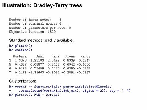
Illustration: Bradley-Terry trees
Number of inner nodes: 3Number of terminal nodes: 4Number of parameters per node: 5Objective function: 1829
Standard methods readily available:R> plot(bt2)R> coef(bt2)
Barbara Anni Hana Fiona Mandy3 1.3378 1.23183 2.0499 0.8339 0.62175 0.4387 0.08877 0.8463 0.6942 -0.10006 0.9475 0.72459 0.4452 0.6350 -0.49657 0.2178 -1.31663 -0.3059 -0.2591 -0.2357
Customization:R> worthf <- function(info) paste(info$object$labels,+ format(round(worth(info$object), digits = 2)), sep = ": ")R> plot(bt2, FUN = worthf)
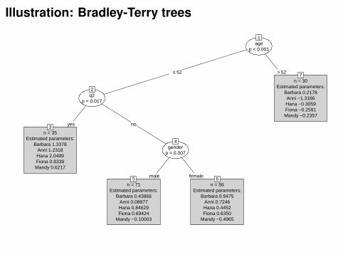
Illustration: Bradley-Terry trees
agep < 0.001
1
≤ 52 > 52
q2p = 0.017
2
yes no
n = 35Estimated parameters:
Barbara 1.3378Anni 1.2318Hana 2.0499Fiona 0.8339Mandy 0.6217
3
genderp = 0.007
4
male female
n = 71Estimated parameters:
Barbara 0.43866Anni 0.08877Hana 0.84629Fiona 0.69424
Mandy −0.10003
5n = 56
Estimated parameters:Barbara 0.9475
Anni 0.7246Hana 0.4452Fiona 0.6350
Mandy −0.4965
6
n = 30Estimated parameters:
Barbara 0.2178Anni −1.3166Hana −0.3059Fiona −0.2591Mandy −0.2357
7

Illustration: Bradley-Terry trees
agep < 0.001
1
≤ 52 > 52
q2p = 0.017
2
yes no
Barbara: 0.19Anni: 0.17Hana: 0.39Fiona: 0.11Mandy: 0.09Anja: 0.05
3
genderp = 0.007
4
male female
Barbara: 0.17Anni: 0.12Hana: 0.26Fiona: 0.23Mandy: 0.10Anja: 0.11
5Barbara: 0.27
Anni: 0.21Hana: 0.16Fiona: 0.19Mandy: 0.06Anja: 0.10
6
Barbara: 0.26Anni: 0.06Hana: 0.15Fiona: 0.16Mandy: 0.16Anja: 0.21
7

Illustration: Bradley-Terry trees3
Objects
Wor
th p
aram
eter
s
0.0
0.1
0.2
0.3
0.4
●●
●
●●
●
Barbara Anni Hana Fiona Mandy Anja
5
Objects
Wor
th p
aram
eter
s
0.0
0.1
0.2
0.3
0.4
●
●
●
●
●●
Barbara Anni Hana Fiona Mandy Anja
6
Objects
Wor
th p
aram
eter
s
0.0
0.1
0.2
0.3
0.4
●
●
●
●
●
●
Barbara Anni Hana Fiona Mandy Anja
7
Objects
Wor
th p
aram
eter
s
0.0
0.1
0.2
0.3
0.4
●
●
● ● ●
●
Barbara Anni Hana Fiona Mandy Anja

Illustration: Bradley-Terry trees
Apply plotting in all terminal nodes:R> par(mfrow = c(2, 2))R> nodeapply(bt2, ids = c(3, 5, 6, 7), FUN = function(n)+ plot(n$info$object, main = n$id, ylim = c(0, 0.4)))
Predicted nodes and ranking:R> tm
age gender q1 q2 q31 60 male no no no2 25 female no no no3 35 female no yes no
R> predict(bt2, tm, type = "node")
1 2 37 3 5
R> predict(bt2, tm, type = function(object) t(rank(-worth(object))))
Barbara Anni Hana Fiona Mandy Anja1 1 6 5 4 3 22 2 3 1 4 5 63 3 4 1 2 6 5

Summary
All new implementation of model-based recursive partitioning inpartykit.
Enables more efficient computations, rapid prototyping, flexiblecustomization.
Some new inference options.

References
Hothorn T, Zeileis A (2014). partykit: A Toolkit for Recursive Partytioning.R package version 0.2-0.URL http://R-Forge.R-project.org/projects/partykit/
Zeileis A, Hothorn T (2014). Parties, Models, Mobsters: A NewImplementation of Model-Based Recursive Partitioning in R.vignette("mob", package = "partykit").
Strobl C, Wickelmaier F, Zeileis A (2011). “Accounting for IndividualDifferences in Bradley-Terry Models by Means of Recursive Partitioning.”Journal of Educational and Behavioral Statistics, 36(2), 135–153.doi:10.3102/1076998609359791
Zeileis A, Hothorn T, Hornik K (2008). “Model-Based Recursive Partitioning.”Journal of Computational and Graphical Statistics, 17(2), 492–514.doi:10.1198/106186008X319331