particle dynamics of matter-wave solitons
TRANSCRIPT

School of Mathematics & Statistics
MMath Project
Particle Dynamics of Matter-WaveSolitons
Author:Imogen Large
Supervisor:Dr. Nick Parker
May 2014

Abstract
Solitons are important in the modelling of nonlinear systems like black holes and fibre-optics,however due to their non-dispersive nature they are difficult to form in practical experiments.Bose-Einstein condensation provides a physical system in which solitons can be observed andcontrolled. To a good approximation the Gross-Pitaevskii equation calculates the dynamics ofa Bose-Einstein condensate theoretically, and an exact soliton solution can be derived. In thisdissertation, Hamiltonian mechanics are used to provide a particle model for various soliton sys-tems. In recent experiments, a Gaussian barrier was introduced into the trapping potential ofa one-soliton system; here the system is modelled theoretically and the results show excellentagreement. Two external potentials are considered in two-soliton systems; the typical interactionpotential between solitons demonstrates the phase-shift, and the Lennard-Jones potential consid-ers the attractive and repulsive forces between solitons. The contrasting nature of these potentialsis observed through simulation and presented in Poincare sections.

Contents
1 Introduction 21.1 Solitons . . . . . . . . . . . . . . . . . . . . . . . . . . . . . . . . . . . . . . . . . 21.2 Solitons in Bose-Einstein Condensates . . . . . . . . . . . . . . . . . . . . . . . . . 4
2 Theory 92.1 Gross-Pitaevskii Equation . . . . . . . . . . . . . . . . . . . . . . . . . . . . . . . 92.2 Hamiltonian Mechanics . . . . . . . . . . . . . . . . . . . . . . . . . . . . . . . . . 12
3 Single Soliton Model 143.1 Dynamics in an Open Space . . . . . . . . . . . . . . . . . . . . . . . . . . . . . . 143.2 Dynamics in a Harmonic Trap . . . . . . . . . . . . . . . . . . . . . . . . . . . . . 143.3 Dynamics in a Harmonic Trap with a Barrier . . . . . . . . . . . . . . . . . . . . . 16
4 Two-Soliton Dynamics:The Interaction Potential 204.1 Short Term Dynamics . . . . . . . . . . . . . . . . . . . . . . . . . . . . . . . . . 214.2 Longer Term Dynamics . . . . . . . . . . . . . . . . . . . . . . . . . . . . . . . . . 234.3 Frequencies . . . . . . . . . . . . . . . . . . . . . . . . . . . . . . . . . . . . . . . 244.4 Poincare Sections . . . . . . . . . . . . . . . . . . . . . . . . . . . . . . . . . . . . 26
5 Two-Soliton Dynamics:The Lennard-Jones Potential 325.1 Short Term Dynamics . . . . . . . . . . . . . . . . . . . . . . . . . . . . . . . . . 335.2 Longer Term Dynamics . . . . . . . . . . . . . . . . . . . . . . . . . . . . . . . . . 355.3 Frequencies . . . . . . . . . . . . . . . . . . . . . . . . . . . . . . . . . . . . . . . 365.4 Poincare Sections . . . . . . . . . . . . . . . . . . . . . . . . . . . . . . . . . . . . 37
6 Summary 41
References 42
1
Chapter 1
Introduction
1.1 Solitons
Solitons, or solitary waves, are localised wave-packets which do not disperse over time. Aregular wave disperses as it propagates and its amplitude decreases; in contrast a solitary waveretains a fixed height and shape despite propagation. Solitons are solutions to nonlinear waveequations describing particle-like waves of energy which are precise and rigorous. Solitary wavesare experimental representations of these solutions, and so can be considered as approximate formsof the analytical solutions. Solitary waves can be applied in the analysis of various nonlinearsystems such as nonlinear optics and shallow water.
Solitons were first observed by John Scott Russell, a civil engineer and naval architect, in 1834on the Union Canal near Edinburgh. He was investigating the most efficient design of canal boatswhen the boat he was observing came to a sudden stop, and the wave at the front of the boatcarried on moving. Russell pursued the wave and this extract from his report details his findings:
“I believe that I shall best introduce this phenomenon by describing the circumstances of myown first acquaintance with it. I was observing the motion of a boat which was rapidly drawn alonga narrow channel by a pair of horses, when the boat suddenly stopped - not so the mass of waterin the channel which it had put in motion; it accumulated round the prow of the vessel in a stateof violent agitation, then suddenly leaving it behind, rolled forward with great velocity, assumingthe form of a large solitary elevation, a rounded, smooth and well-defined heap of water, whichcontinued its course along the channel apparently without change of form or diminution of speed.I followed it on horseback, and overtook it still rolling on at a rate of some eight or nine miles anhour, preserving its original figure some thirty feet long and a foot to a foot and a half in height.Its height gradually diminished, and after a chase of one or two miles I lost it in the windings ofthe channel. Such, in the month of August 1834, was my first chance interview with that singularand beautiful phenomenon which I have called the Wave of Translation, a name which it now verygenerally bears.” [1]
The “Wave of Translation” witnessed by Russell did not decrease in height or speed butcontinued to propagate with its original profile. This gives reason for us to believe he did indeedobserve a soliton. Russell continued his investigations into the “beautiful phenomenon”, recreatingthe wave using a plate which formed a division across a long narrow channel of shallow water [1].Russell [2] extracted some essential properties of the wave of translation, two of which are
2

CHAPTER 1. INTRODUCTION
� “the higher wave moves more rapidly than the lower” and
� “the great primary waves of translation cross each other without change of any kind”.
Precise definitions of solitons are difficult to find, and therefore, in this report, we definesolitons based on properties given by Drazin and Johnson [3]. A soliton is any solution of anonlinear equation (or system) which (i) represents a wave of permanent form; (ii) is localised, sothat it decays or approaches a constant at infinity; (iii) can interact strongly with other solitonsand retain its identity.
The crucial feature is that these waves interact strongly and then continue to propagate withalmost no interaction. We consider a system of two solitons of different amplitudes travelling inthe same direction [4]. They are placed with sufficient gap between them such that their tailsdon’t overlap. As the taller wave catches up with the shorter one, we may have expected thewaves to combine in some way but this is not the case. Both solitons emerge unchanged fromthe interaction. They both retain their form, amplitude and speed and there is a slight shift inposition. This property is more comparable to that of a particle. This gives the wave particle-like characteristics, emphasised when Zabusky and Kruskal [5] named the waves ‘solitons’ (afterprotons, photons, etc.).
1.1.1 Wave Equations
We consider the classical wave equation,
utt − c2uxx = 0 (1.1)
where u(x, t) is the amplitude of the wave, c is a constant with c > 0 and the subscript denotes thepartial derivative. Equation (1.1) is a linear wave equation which describes a wave propagating ina vacuum without dissipative effects. The wave disperses as it propagates. We wish to describe awave without dispersion and so look to include nonlinearities which balance the dispersive effects.
As discovered by John Scott Russell, solitons have been seen and reproduced in shallow waterdynamics. In 1895, Korteweg and de-Vries [6] derived this equation to describe these waves,
ut + (1 + u)ux + uxxx = 0. (1.2)
which includes a nonlinearity in its simplest form and is known as the KdV equation. The nonlinearpartial differential equation can be solved using the inverse scattering transform. This methodcan be applied to nonlinear integrable systems and used to give exact solutions.
Travelling waves in shallow water are described such that the top of the peak is travellingfaster than the bottom. This causes the wave to break. Korteweg and de-Vries were interestedin exploring if long water waves continued to “steepen in front and become less steep behind” [4].They showed that the KdV equation has steady progressing wave solutions,
u(x, t) = −1
2a2 sech2
[1
2a(x− x0 − a2t
)]. (1.3)
The velocity a2 is proportional to the amplitude. The width is inversely proportional to thesquare root of the amplitude. Thus we know that taller solitary waves travel faster and arenarrower than shorter ones [4], confirming the characteristic given by Russell [2].
3

CHAPTER 1. INTRODUCTION
Another nonlinear model that supports soliton solutions, more relevant to our study, is thenonlinear Schrodinger Equation. Originally arising in the theory of superconductivity and later inthe theory of superfluidity [3], the NLS equation is given by
iut +1
2uxx + |u|2u = 0. (1.4)
Like the KdV equation, the NLS equation can be applied to packets of water waves andadditionally plasma waves. The most important applications of the NLS equation is in the field ofnonlinear optics. It was first suggested in 1973 that optical fibres could support solitons pulses [7,8].At the time, fibre optics research was focussed on reducing the levels of information lost over largedistances and solitons offered a solution [9]. Since then solitons have proved crucial in preservinga signal through fibre optics. The NLS equation is relevant for modelling solitons in Bose-Einsteincondensates which we explore further in this dissertation.
1.2 Solitons in Bose-Einstein Condensates
1.2.1 Quantum Particles and Wave-Particle Duality
The dynamics of everyday objects around us can be modelled by classical mechanics howeverthis is not sufficient for particles or objects of such a tiny scale. The behaviour of quantumparticles is subject to quantum mechanics which provides a framework for describing dynamicsat the subatomic lengthscale. Heisenburg’s uncertainty principle states that it is not possible toknow the position and velocity of a particle simultaneously [10], and therefore the position andvelocity of quantum particles are each defined by a probability distribution. This uncertainty givesthe particles a degree of ‘blurriness’ as their exact positions and velocities are not known. The‘blurriness’ in position is described by the de Broglie wavelength, λdB. Since quantum particlesare defined to have this wavelength, they possess the properties of waves as well as particles; thisis called wave-particle duality.
All particles can be classified as either bosons or fermions. The distinction is important because,due to their distinguishing properties, the behaviour of a gas of bosons differs greatly from fermionicgases. Bosons are particles with integer spin (with angular momentum 0, 1, 2, 3, ...); fermionshave half-integer spin (1/2, 3/2, 5/2, ...) [11]. Examples of fermions include fundamental particles,electrons, neutrons and protons. Fermions cannot occupy the same quantum state at the sametime; they are unsociable. Combining an even number of fermions forms a composite particle withinteger spin, a boson. Photons and the majority of atoms are examples of bosons. Bosons areable to occupy the same quantum state and are sociable in nature. The solitons described in thisdissertation are produced in a gas which exploits the social nature of bosons.
1.2.2 Bose-Einstein Condensates
A quantum gas is a gas where quantum mechanics rather than Newtonian mechanics dominatesthe behaviour of the particles. Quantum gases are formed at cold temperatures, at less than 1millionth of a degree above absolute zero (0 Kelvin (K) or -273°C).
Einstein [12] was interested in how the sociable nature of the bosons could be applied and firsttheorised a quantum mechanical phenomenon called Bose-Einstein condensation in 1925 usingBose’s newly theorised statistics for quantum particles. It wasn’t until 1995 that it was realisedin weakly interacting atomic gases [13].
4

CHAPTER 1. INTRODUCTION
Consider a system of a fixed number of atoms with a fixed total energy. The sociable bosonproperty allows the atoms to be in any state within the system. The particles have an averageseparation d and velocity v.
Figure 1.1: The diagram explains criterion for Bose-Einstein condensation [14].
At relatively high temperatures the particles move around randomly with high velocities,bouncing off each other like snooker balls and d is large, as shown in the first panel of Figure1.1. If or when they collide, the particles behave classically. The temperature decreases and theparticles begin to behave more like waves (panel 2). Each wave-packet is localised with a sizegiven by the de Broglie wavelength,
λdB =h
m|v|∝ T−1/2, (1.5)
where h ≈ 6.67× 10⁻³⁴Js is Planck’s constant, m is the mass of the particle, v is the velocity andT is the temperature of the system. The temperature decreases, tending towards absolute zero,and the particles are moving slower. As |v|→ 0, the wavelengths of each particle increases. As thegas is cooled the number of atoms in the lowest energy state of the system gets bigger. When thesystem reaches a critical temperature, TC , the size of the wave-packets increases to the extent thatλdB ≈ d, and the particles start to overlap, as shown in panel 3. As they overlap they combine toform a giant matter wave across the whole system. Within the huge wave individual particles canno longer be identified and the atoms behave as one. At T = TC the number of particles in thelowest energy state increases significantly forming a spike in the energy distribution, see Figure1.2. This is a Bose-Einstein condensate. At T = 0 all the particles fall into the ground energystate and this is a pure Bose-Einstein condensate, depicted in the final panel of Figure 1.1.
Bose-Einstein condensation can occur in other scenarios. The condensation occurs when thewave-packets overlap. This happens either at very low temperatures (as detailed above) or at veryhigh densities. An example of the second case is neutron stars where the density of particles is sogreat that the particles are forced so close together that they overlap.
Quantum physics, due to its definition, is too small to be observed easily. Bose-Einsteincondensation offers the chance to view particles conforming to quantum mechanics on a largerscale. In the current pursuit of the quantum ‘era’, manipulation of BECs is crucial to the progress
5

CHAPTER 1. INTRODUCTION
Figure 1.2: First weakly interacting atomic Bose-Einstein Condensate realisation by Cornell et al. [11]who received a Nobel Prize in Physics 2001.
of this research. BECs are nonlinear systems; this is important as it provides a platform toinvestigate nonlinear objects such as investigate solitons.
1.2.3 Solitons in Bose-Einstein Condensates
Solitons arise in BECs in two forms which is determined by atomic interactions within thecondensate [15]. The interactions introduce the nonlinearity into the system which balances thedispersion. In the absence of interactions, there is no nonlinearity and therefore no soliton in thecondensate.
The particles in the BEC have a weak interaction between each other which is only felt whenthey are close together. The interaction is still effective, despite the weakness, due to the verycold temperatures and very low energy in the system. The consequence of the atoms being soclose together is an energetic cost for the interaction, g, defined as
g =4πh2asm
, (1.6)
where h is reduced Planck’s constant, as is the s-wave scattering length and m is the mass of eachatom. The scattering length is the critical distance between the atoms when an interaction occurs.Experimentalists can control the magnitude and sign of as and therefore g, and so can determinethe interactions between the atoms.
� g > 0 : repulsive interactions; it costs the system energy to keep the atoms close together.
� g = 0 : no interactions and no nonlinearity.
� g < 0 : attractive interactions; it reduces the energy in the system as the atoms are alreadyclose together.
Formed in a BEC with repulsive interactions, dark solitons are localised, negative dips inamplitude which satisfy the defining properties of solitons [3]. Contrastingly bright solitons appear
6

CHAPTER 1. INTRODUCTION
in BECs with attractive interactions. They are localised bumps in the condensate similar to pulsesof light. The attractive interactions allow the bright soliton to retain its profile without dispersingdespite propagation. In this dissertation, we consider bright solitons in Bose-Einstein condensateswith attractive atomic interactions. Being able to control the interactions within the BEC allowssystems to be constructed that are advantageous for modelling nonlinear systems like solitons.Solitons can be studied experimentally in systems of water or optics, but the unique properties ofthe BECs allow the solitons to last indefinately.
atoms, >2/3, remains in a noncondensedpedestal around the soliton, clearly visiblefor intermediate propagation times in theguide.
We then made measurements of the wave-packet size versus propagation time for threevalues of the scattering length: a > 0, a >20.11 nm, and a > 20.21 nm (Fig. 4). For a> 0 (Fig. 4A), the interaction between atomsis negligible, and the size of the cloud isgoverned by the expansion of the initial con-densate distribution under the influence of thenegative curvature of the axial potential. Themeasured size is in excellent agreement withthe predicted size of a noninteracting gassubjected to an expulsive harmonic potential:Taking the curvature as a fit parameter (solidline in Fig. 4A), we find vz 5 2ip 3 78(3)Hz, which agrees with the expected value ofthe curvature produced by the pinch coils(14). For a 5 20.11 nm and B 5 487 G, thesize of the wave packet is consistently belowthat of a noninteracting gas (Fig. 4B, solidline). Attractive interactions reduce the sizeof the atomic cloud but are not strong enoughto stabilize the soliton against the expulsivepotential. When a is further decreased to20.21 nm, the measured size of the wavepacket no longer changes as a function ofguiding time, indicating propagation withoutdispersion even in the presence of the expulsivepotential (Fig. 4C).
To theoretically analyze the stability ofthe soliton, we introduce the 3D Gross-Pitaevskii energy functional
EGP 5 * d3r\2
2m¹C~rW!2 1
Ng
2C (rW)4
11
2m @v'
2 ~ x21y2! 1 vz2z2#C~rW!2
(1)
where the condensate wave function C isnormalized to 1. In Eq. 1 the first term is thekinetic energy responsible for dispersion; thesecond term is the interaction energy, whichin the present case of attractive effective in-teractions (g , 0) causes the wave function tosharpen; and the third term is the externalpotential energy. We introduce the followingtwo-parameter variational ansatz to estimateminimal-energy states of EGP:
C~rW! 51
Î2ps'2 lz
1
cosh~z/lz!
expS2 x2 1 y2
2s'2 D (2)
where s' and lz are the radial and axialwidths of the wave function. The functionalform of the well-known 1D soliton has beenchosen for the longitudinal direction (5),while in the transverse direction a Gaussianansatz is the optimal one for harmonic con-
finement. For each lz we minimize the meanenergy over s'; the resulting function of lz isplotted (Fig. 5) for various values of theparameter Na/a'
ho where a'ho 5 (\/mv')1/2.
For very small axial sizes, the interactionenergy becomes on the order of 2\ v' andthe gas loses its quasi-1D nature and collaps-es (3, 4). For very large axial sizes, theexpulsive potential energy dominates andpulls the wave function apart. For intermedi-ate sizes, attractive interactions balance boththe dispersion and the effect of the expulsivepotential; the energy presents a local mini-mum (solid line in Fig. 5). This minimumsupports a macroscopic quantum bound state.However, it exists only within a narrow win-dow of the parameter Na/a'
ho. In our experi-ments v' 5 2p 3 710 Hz and vz 5 2ip 370 Hz for B 5 420 G, so that a'
ho 5 1.4 mm;for Na larger than (Na)c 5 1.105 mm, acollapse occurs (dashed curve in Fig. 5),while for Na smaller than (Na)e 5 0.88mm the expulsive potential causes the gas toexplode axially (dotted curve in Fig. 5).
For our experimental conditions and a 520.21 nm, the number of atoms that allows thesoliton to be formed is 4.2 3 103 # N # 5.2 3103, in good agreement with our measurednumber 6(2) 3 103. The expected axial size ofthe soliton is lz > 1.7 mm, which is below thecurrent resolution limit of our imaging system.To verify the presence of a critical value ofNae needed to stabilize the soliton, we haveperformed the measurements with the same abut with a reduced number of atoms, N 5 2 3103. At 8 ms guiding time the axial size of thewave packet increased to 30 mm, indicating thatno soliton was formed.
One may speculate as to the formation dy-namics of the soliton in the elongated trapbefore its release in the optical waveguide. Be-cause the atom number in the initial BEC, 2 3
Fig. 5. Theoretical energy diagram of an attrac-tive Bose gas subjected to an expulsive poten-tial for vz/v' 5 i 3 70/710. The energy as afunction of the axial size after minimizationover the tranverse size is shown for three val-ues of Na: within the stability window (solidcurve), at the critical point for explosion(Na)e (dotted curve), and at the critical pointfor collapse (Na)c (dashed curve). End pointsof the curves indicate collapse, i.e., s' 5 0.
Fig. 3. Absorption im-ages at variable delaysafter switching off thevertical trapping beam.Propagation of an idealBEC gas (A) and of asoliton (B) in the hori-zontal 1D waveguide inthe presence of an ex-pulsive potential. Prop-agation without disper-sion over 1.1 mm is aclear signature of asoliton. Correspondingaxial profiles are inte-grated over the verticaldirection.
A B CFig. 4. Measured rootmean square size of theatomic wave packetGaussian fit as a func-tion of propagationtime in the waveguide.(A) a 5 0, ideal gascase; (B) a 5 20.11nm; (C) a 5 20.21 nm;solid lines: calculatedexpansion of a nonin-teracting gas in the ex-pulsive potential.
R E P O R T S
17 MAY 2002 VOL 296 SCIENCE www.sciencemag.org1292
Figure 1.3: Matter-wave bright soliton as produced by Khaykovich et al. [16]. Panel A shows a systemwith g = 0, and the soliton disperses. Panel B is a system with attractive interactions and the profile ofthe soliton is maintained.
prevent the condensate from moving under the influence of theinfrared potential until, at a certain instant, the end caps are switchedoff and the condensate is set in motion. The condensate is allowed toevolve for a set period of time before an image is taken. As shown inFig. 3, the condensate spreads for a . 0, while for a , 0, non-spreading, localized structures (solitons) are formed. Solitonshave been observed for times exceeding 3 s, a limitation that webelieve is due to loss of atoms rather than wave-packet spreading.
Multiple solitons (‘soliton trains’) are usually observed, as isevident in Figs 3 and 4. We find that typically four solitons arecreated from an initially stationary condensate. Although multi-soliton states with alternating phase are known to be stationarystates of the nonlinear Schrodinger equation14,22,23, mechanisms fortheir formation are diverse. It was proposed that a soliton traincould be generated by a modulational instability24, where in the caseof a condensate, phase fluctuations would produce a maximumrate of amplitude growth at a wavelength approximately equal tothe condensate healing length y ¼ (8pnjaj)21/2, where n is theatomic density23. As a and y are dynamically changing in theexperiment, the expected number of solitons N s is not readilyestimated from a static model. Experimentally, we detect no
significant difference in N s when the time constant, t, for changingthe magnetic field is varied from 25 ms to 200 ms. We investigatedthe dependence of N s on condensate velocity v by varying theinterval Dt between the time the end caps are switched off to thetime when a changes sign. We find that N s increases linearly with Dt,from ,4 at Dt ¼ 0 to ,10 at Dt ¼ 35 ms. As the axial oscillationperiod is ,310 ms, v / Dt in the range of Dt investigated.
The alternating phase structure of the soliton train can beinferred from the relative motion of the solitons. Non-interactingsolitons, simultaneously released from different points in a harmo-nic potential, would be expected to pass through one another. Butthis is not observed, as can be seen from Fig. 4, which shows that thespacing between the solitons increases near the centre of oscillationand bunches at the end points. This is evidence of a short-rangerepulsive force between the solitons. Interaction forces betweensolitons have been found to vary exponentially with the distancebetween them, and to be attractive or repulsive depending on theirrelative phase25. Because of the effect of wave interference on thekinetic energy, solitons that differ in phase by p will repel, whilethose that have the same phase will attract. An alternating phasestructure can be generated in the initial condensate by a phase
0 ms
150
300
500
635
1,260
1,860
a > 0 a < 0
Figure 3 Comparison of the propagation of repulsive condensates with atomic solitons.
The images are obtained using destructive absorption imaging, with a probe laser detuned
27 MHz from resonance. The magnetic field is reduced to the desired value before
switching off the end caps (see text). The times given are the intervals between turning off
the end caps and probing (the end caps are on for the t ¼ 0 images). The axial dimension
of each image frame corresponds to 1.28 mm at the plane of the atoms. The amplitude of
oscillation is ,370 mm and the period is 310 ms. The a . 0 data correspond to 630 G,
for which a < 10a o, and the initial condensate number is ,3 £ 105. The a , 0 data
correspond to 547 G, for which a < 2 3a o. The largest soliton signals correspond to
,5,000 atoms per soliton, although significant image distortion limits the precision of
number measurement. The spatial resolution of ,10 mm is significantly greater than the
expected transverse dimension l r < 1.5 mm.
5 ms
70 ms
150 ms
Figure 4 Repulsive interactions between solitons. The three images show a soliton train
near the two turning points and near the centre of oscillation. The spacing between
solitons is compressed at the turning points, and spread out at the centre of the oscillation.
A simple model based on strong, short-range, repulsive forces between nearest-
neighbour solitons indicates that the separation between solitons oscillates at
approximately twice the trap frequency, in agreement with observations. The number of
solitons varies from image to image because of shot to shot experimental variations, and
because of a very slow loss of soliton signal with time. As the axial length of a soliton is
expected to vary as 1/N (ref. 11), solitons with small numbers of atoms produce
particularly weak absorption signals, scaling as N 2. Trains with missing solitons are
frequently observed, but it is not clear whether this is because of a slow loss of atoms, or
because of sudden loss of an individual soliton.
letters to nature
NATURE | VOL 417 | 9 MAY 2002 | www.nature.com152 © 2002 Macmillan Magazines Ltd
Figure 1.4: Soliton train as produced by Strecker et al. [17]. The group of solitons propagate withoutcombining or dispersing.
In 2002 bright solitons were formed in two separate experiments. Khaykovich et al. [16] pro-duced matter-wave bright solitons in an ultracold lithium-7 gas. They compared results of twosystems with different scattering lengths as shown in Figure 1.3. The propagation of an ideal gas,where g = 0, results in the BEC dispersing. In the system with attractive interactions, the BECpropagated without dispersion over 1.1mm, giving the indication of a soliton.
Simultaneously at Rice University, Strecker et al. [17] formed matter-wave soliton trains. Agroup of bright solitons of lithium-7 atoms in a quasi-1D waveguide were observed to propagatewithout spreading for many oscillatory cycles, as shown in Figure 1.4. The solitons did not mergetogether due to the relative phase, which was set to be φ = π.
7
CHAPTER 1. INTRODUCTION
In 2013 physicists at Durham University formed a Rubidium BEC containing a bright solitarymatter-wave. Marchant et al. examined the reflection of the soliton from a Gaussian barriercontained within a harmonic trap [18]. They observed experimentally the effects the barrier hadon the dynamics of the soliton and in Section 3.3 we recreate their results in a numerical model.
There is currently much theoretical interest in the stability of solitons in collisions and how thesetheories can be applied in physical systems [15]. A potential application for bright solitons in BECsis interferometry, a method for extracting information about forces. Experiments have previouslyrelied on manipulating waves of light and precision in measurements was poor. The properties ofbright solitary waves offer the opportunity for improving the precision. Interferometers are able tosplit the BEC and recombine it after a period. Differences in properties and phase give indicationto the conditions of the separate paths which the split BEC takes. This technique of investigationis important in applications to astronomy, oceanography and fibre optics.
There are two main ways to model solitons theoretically. An analytical soliton solution to thenonlinear wave equation can be found and solved in very limited cases, e.g. for a stationary soliton,but we are interested in more dynamical systems. Since solitons do not experience dispersion, theycan be modelled as particles in a much simpler system. Hamiltonian mechanics are a platformused for modelling the quantum mechanics of solitons numerically. Although this method neglectsthe internal excitations of solitons, it allows us to calculate soliton trajectories without having tosolve the full nonlinear wave equation. Martin et al. [19] show that the classical particle dynamicalmodel shows good agreement with the full solution of the wave equation. This classical particlemodel is what we develop further in this dissertation.
8
Chapter 2
Theory
2.1 Gross-Pitaevskii Equation
To a good approximation the dynamics of a BEC can be described by the Gross-PitaevskiiEquation [20, 21], the GPE, which is a specific form of the nonlinear Schrodinger equation. Itis a classical wave equation which arises from an approximation to the Heisenberg equations ofmotion [22]. The Gross-Pitaevskii equation in three dimensions is
ih∂
∂tΨ(r, t) =
(− h2
2m∇2 + V (r) + g3DN |Ψ(r, t)|2
)Ψ(r, t), (2.1)
where Ψ(r, t) denotes the wave-function and h is the reduced Planck’s constant. The mass of eachparticle is given by m, g3D is the strength of interaction, N is the number of particles in the BECand V (r) is the trapping potential. The trapping potential is a magnetic field which holds theBEC in space. It can be varied in time and space to manipulate the BEC. For convenience thewave-function is normalised to one. The GPE is a valid description given that the condensate ismacroscopically populated N � 1 and the temperature of the gas is sufficiently low that T � TCholds.
Time independent solutions of the GPE have the form
Ψ(r, t) = ψ(r)e−iµth (2.2)
where ψ(r) is time-independent and µ is the chemical potential (constant), the energy required toadd or remove a particle from the system. Substituting this expression into Equation (2.1) givesthe time-independent form of the GPE as
µψ(r) =
(− h2
2m∇2 + V (r) + g3DN |ψ(r)|2
)ψ(r), (2.3)
solutions to which describe the stationary states of the system.
2.1.1 Trapping Potentials
BECs are typically confined by harmonic potentials, or traps, which have the general form
V (r) =m
2
(ω2xx
2 + ω2yy
2 + ω2zz
2), (2.4)
9
CHAPTER 2. THEORY
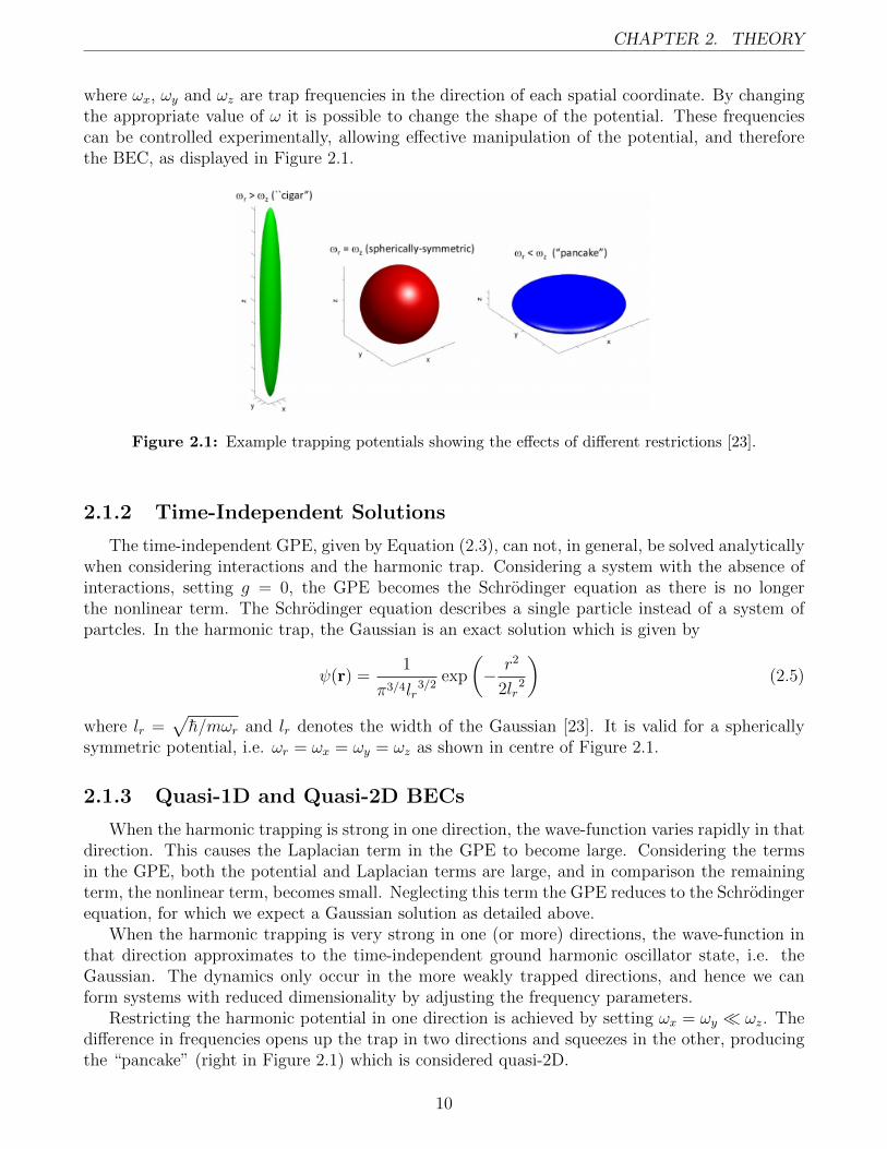
where ωx, ωy and ωz are trap frequencies in the direction of each spatial coordinate. By changingthe appropriate value of ω it is possible to change the shape of the potential. These frequenciescan be controlled experimentally, allowing effective manipulation of the potential, and thereforethe BEC, as displayed in Figure 2.1.
Figure 2.1: Example trapping potentials showing the effects of different restrictions [23].
2.1.2 Time-Independent Solutions
The time-independent GPE, given by Equation (2.3), can not, in general, be solved analyticallywhen considering interactions and the harmonic trap. Considering a system with the absence ofinteractions, setting g = 0, the GPE becomes the Schrodinger equation as there is no longerthe nonlinear term. The Schrodinger equation describes a single particle instead of a system ofpartcles. In the harmonic trap, the Gaussian is an exact solution which is given by
ψ(r) =1
π3/4lr3/2
exp
(− r2
2lr2
)(2.5)
where lr =√h/mωr and lr denotes the width of the Gaussian [23]. It is valid for a spherically
symmetric potential, i.e. ωr = ωx = ωy = ωz as shown in centre of Figure 2.1.
2.1.3 Quasi-1D and Quasi-2D BECs
When the harmonic trapping is strong in one direction, the wave-function varies rapidly in thatdirection. This causes the Laplacian term in the GPE to become large. Considering the termsin the GPE, both the potential and Laplacian terms are large, and in comparison the remainingterm, the nonlinear term, becomes small. Neglecting this term the GPE reduces to the Schrodingerequation, for which we expect a Gaussian solution as detailed above.
When the harmonic trapping is very strong in one (or more) directions, the wave-function inthat direction approximates to the time-independent ground harmonic oscillator state, i.e. theGaussian. The dynamics only occur in the more weakly trapped directions, and hence we canform systems with reduced dimensionality by adjusting the frequency parameters.
Restricting the harmonic potential in one direction is achieved by setting ωx = ωy � ωz. Thedifference in frequencies opens up the trap in two directions and squeezes in the other, producingthe “pancake” (right in Figure 2.1) which is considered quasi-2D.
10

CHAPTER 2. THEORY
For a quasi-1D trap, the potential is restricted in two directions with ωx = ωy � ωz, producingthe “cigar” (left in Figure 2.1). The high frequencies squeeze the trap radially and the condensateand trap can be considered to be in one dimension. We proceed by considering a quasi-1D systemin x and so the potential V (r) becomes V (x) = mω2
xx2/2.
2.1.4 One-Dimensional Gross-Pitaevskii Equation
To produce one dimensional objects like solitons, the dynamical system should have the samedimensional properties. We can draw simpler conclusions more efficiently by reducing the three di-mensional GPE to an equation with only one spatial coordinate [22]. To obtain the one-dimensionalGPE analytically, we take this decomposition of the wave-function in the y and z directions,
Ψ(r, t) = ψ(x, t)Φ(y)Φ(z) where Φ(ζ) =
(1
σ2π
)1/4
exp
(− ζ2
2σ2
). (2.6)
The wave-function has a Gaussian form with σ2 = h/mωr [19] and we can integrate out in they and z directions by applying the operator
∞∫−∞
∞∫−∞
Φ∗(y)Φ∗(z)dydz. (2.7)
which “averages” the wave-function in the radial directions. Applying restrictions (as defined inSection 2.1.3) to the potential so that it is sufficiently tight in the y and z directions, the harmonictrap potential energy is effective only in the x direction. And so (2.1) becomes
ih∂
∂tψ(x, t) =
(− h2
2m
∂2
∂x2+mω2
xx2
2+ g1DN |ψ(x, t)|2+hωr
)ψ(x, t). (2.8)
noting here how the derivatives are now only in x and the strength of interaction has changed toreflect the reduction in dimension.
The dimensionless form of the GPE allows us to find the simplest numerical form of thesolution. Introducing the dimensionless variables
x =m|g1D|N
h2x, t =
m|g1D|2N2
h3t,
(2.9)
ω =h3
m|g1D|2N2ωx, ψ(x) =
h√mg1DN
Ψ(x).
Equation (2.8) becomes
i∂
∂tψ(x, t) =
[−1
2
∂2
∂x2+
1
2ω2x2 − |ψ(x, t)|2
]ψ(x, t). (2.10)
Applying the same relations to the time-independent GPE, we obtain
µψ(x) =
[−1
2
∂2
∂x2+
1
2ω2x2 − |ψ(x)|2
]ψ(x). (2.11)
11

CHAPTER 2. THEORY
Now that every variable is dimensionless we proceed using these quantities and can remove the‘tilde’ notation. Considering a system in open space, with no potential (ω = 0), we seek a solutionof the dimensionless form ψ(x, t) = ψ(x)e−iµt. We take the trial solution,
ψ (x) = A sechx
Bwhich gives ψ (x) =
√2|µ| sech
(√2|µ|x
). (2.12)
The sech form of the solution demonstrates the wave is localised in nature. The solutionis time-independent and there is no trapping along x and so the wave is held together by theattractive interactions only. Hence it is a soliton solution.
−5 −4 −3 −2 −1 0 1 2 3 4 50
0.5
1
1.5
x
ψ(x
)
µ = −1
µ = −0.75
µ = −0.5
Figure 2.2: The exact soliton solution to the GPE for different values of µ.
2.1.5 The Effective Mass
Following methods used by Martin et al. in [19] the wave-function is normalised to one. Thenorm is given by
N =
∞∫−∞
|ψ (x) |2dx = 4η (2.13)
which is set such that N = 1. So when considering a one soliton system, η = 0.25; for two solitonsη1 = η2 = 0.125.
2.2 Hamiltonian Mechanics
To avoid solving the full GPE to calculate the trajectories of the soliton, we use Hamiltonianmechanics as a platform for modelling the motion numerically. The exact solution given byEquation (2.12) confirms the localised nature of the solitary wave solution such that we can modelit as a particle. Hamiltonian mechanics allows us to derive equations of motion so we can considerthe particle dynamics within various systems. This classical particle approximation has beenshown to agree well with full numerical solutions of the GPE by Martin et al. [19].
The Hamiltonian describes the energies of the system; remaining constant, H is the sum ofthe kinetic and potential energies. When considering a system with one soliton, the Hamiltonianis given by,
H =p2
2η+
1
2ηω2q2. (2.14)
12

CHAPTER 2. THEORY
The Hamiltonian is given as a function of position q and momentum p; this is reflected in howthe kinetic and potential energies are expressed. Equation (2.14) is appropriate for a simple systemwhich models the particle dynamics of a single soliton in a harmonic trap. The first term refers tothe kinetic energy, the second term the potential energy. This is the relevant potential energy fora harmonic trap with frequency ω. There is an individual Hamiltonian for each respective systemof solitons.
Hamilton’s equations are applied to the Hamiltonian and we obtain equations of motion. Theequations describe the motion of the particle as a coupled system of two first order differentialequations,
dq
dt=∂H
∂pand
dp
dt= −∂H
∂q. (2.15)
They can be considered as giving, at each point (q, p) of phase space, the velocity vector (q, p)used for building all the trajectories (q(t), p(t)) [24]. Upon solving these ODEs, we can obtainvalues for position and momentum of the particle at each time step. Typically we solve the ODEsnumerically using MATLAB.
13

Chapter 3
Single Soliton Model
As motivation for our modelling, we aim to recreate an experiment recently completed byMarchant et al. [18]. The experiment mapped the dynamics of a soliton contained in a harmonicpotential with a barrier in the trap wall. We explore to what extent these results can be foundnumerically. In this chapter we investigate the dynamics of the particle for different systems,increasing the complexity of the potential each time.
3.1 Dynamics in an Open Space
Consider a system with no trapping potential; a soliton is moving in a completely flat openspace. Without any potential, the Hamiltonian is given by H = p2/2η which is independent oftime. It follows that the motion of the particle in this system is trivial as it would remain constantand not change in direction or speed at all as time propagates.
3.2 Dynamics in a Harmonic Trap
For a non-trivial system we introduce a harmonic trapping potential as described in Section2.1.3. For our one dimensional system our potential is given by
V (q) =1
2ηω2q2 (3.1)
where η is the effective mass, ω is the trap frequency and q is the position of the particle. For thissystem we obtain the Hamiltonian,
H =p2
2η+ηω2q2
2, (3.2)
which we solve to obtain Hamilton’s Equations:
dp
dt= −ηω2q2 and
dq
dt=p
η. (3.3)
These coupled ordinary differential equations can be solved analytically. Combining them weobtain this second order ODE, q + ω2q = 0, which describes the motion of the particle. Thesolution is given by
q(t) = A sinωt+B cosωt (3.4)
14

CHAPTER 3. SINGLE SOLITON MODEL
where A and B are constants to be determined by initial conditions. The system is an example ofa simple harmonic oscillator; the trajectory of motion for the soliton is sinusoidal about the originof the trap.
Having obtained a solution for the system analytically, we simulate these results numericallyusing MATLAB to validate the code and accuracy of the ODE solver. As we are following theexperiment which includes the barrier, we keep the trap frequency consistent with that given byMarchant et al. [18]. Taking the experimental value, we apply the dimensionless variables givenin Equation (2.9) to convert into dimensionless values suitable for our model. We set the trapfrequency as specified by [18], ω = 0.03, and the effective mass η = 0.25.
−1 −0.5 0 0.5 10
0.5
1
1.5
x 10−4
q
V(q
)
Figure 3.1: Plot of harmonic trapping potential. The green cross represents the initial position of case1, and the blue cross for case 2.
We consider one soliton in two cases with different initial conditions as shown by the crossesin Figure 3.1;
1. Soliton placed in the centre of the trap, with momentum: q(0) = 0, p(0) = 0.0075 (green);
2. Soliton placed up the trap wall, without momentum: q(0) = −1, p(0) = 0 (blue).
We solve Hamilton’s Equations for each of these cases as shown in Figure 3.2.
Case 1: q(0) = 0, p(0) = 0.0075
The simulation for the first set of initial conditions is represented by the blue line in Figure 3.2.We consider the motion of the soliton as it is placed at the origin in the centre of the harmonictrap. The soliton begins with a small momentum and travels up the wall of the trap. As it movesup, the soliton loses kinetic energy but gains potential energy. At t ≈ 100 the soliton reaches itsmaximum height up the trap wall and is stationary. The soliton then begins to accelerate backdown the trap wall to the centre of the trap, losing potential energy and gaining kinetic energy.As it travels up the opposite side the soliton decelerates again. This motion continues in theform of an oscillation with a sinusoidal shape. We obtain the exact solution for this trajectory;recalling Equation (3.4) we apply our initial conditions and calculate for case 1 q(t) = sinωt. Thisanalytical solution follows the blue trajectory in Figure 3.2 exactly.
15

CHAPTER 3. SINGLE SOLITON MODEL
0 100 200 300 400 500 600 700 800 900 1000−1
−0.5
0
0.5
1
t
q
Figure 3.2: A position - time plot of a single soliton in a symmetric harmonic trap for differing sets ofinitial conditions. Following conditions set by Marchant et al. [18] ω = 0.03.
Case 2: q(0) = −1, p(0) = 0
The green line in Figure 3.2 depicts the simulation for the second set of initial conditions. Weconsider the motion of the soliton as it is displaced from the origin; placed at position q = −1 thesoliton begins the its trajectory up the trap wall with potential energy and no kinetic energy. Thesoliton travels down the trap wall, accelerating it gains kinetic energy and losing potential energy.The soliton passes through the origin and starts decelerating as it travels up the opposite trapwall. At t ≈ 230 the soliton reaches its maximum height and is stationary. It then travels backdown the trap wall and the oscillation forms. As before we compare with the analytical solution.Having applied this set of initial conditions we obtain that for case 2 q(t) = − cosωt.
As a check, we calculate the overall energy of the system at each time interval. We requirethe energy level to remain constant however there is a slight decrease in energy over time. Therelative error is 0.0017 therefore we can conclude that there is no significant loss of energy fromthe system. It is concluded that these errors originate from a relative tolerance level built into theODE45 solver in MATLAB. Decreasing the tolerance improves the results.
3.3 Dynamics in a Harmonic Trap with a Barrier
3.3.1 The Experimental Potential
The introduction of the barrier into the trapping potential complicates the system and makesour results more interesting. To include the Gaussian barrier in the trap we add the barrier termto expression for the potential.
V (q) =mω2q2
2+ V0 exp
[−(q − q0)2
w2
](3.5)
where V0 is the barrier height, w the barrier width and q0 is the barrier position. These parametersallow us to adjust the shape and size of the barrier, and therefore adjust the effects the barriercan have on the motion of the soliton. The conditions chosen ensure the barrier is much wider
16

CHAPTER 3. SINGLE SOLITON MODEL
than the solitary wave and so the wave behaves classically. As before we use the dimensionlessvariables given in Equation (2.9) to convert the experimental values given by Marchant et al. [18]into dimensionless values, suitable for our model. In Figure 3.3 the Gaussian barrier can be seen;the black line represents the shape of the transformed potential; the red dotted line shows theoriginal potential from Section 3.2; the blue cross is the initial starting point of the soliton inthe system. This initial position is clearly chosen to be above the barrier on the trap wall, i.e.|q(0)|> |q0|.
−1500 −1000 −500 0 500 1000 15000
50
100
150
200
250
300
q
V(q
)
(a)
−1500 −1000 −500 0 500 1000 15000
50
100
150
200
250
300
qV
adj(q
)
(b)
Figure 3.3: Plot of the harmonic trap with barrier for (a) original model with conditions based onthose used by [18]: ω = 0.03, V0 = 119, w = 98, q0 = −1135; (b) adjusted model with conditions:ω = 0.0326, V0 = 140, w = 75, q0 = −1135.
3.3.2 Comparison to Experimental Dynamics
Having set the conditions we proceed with the theoretical simulation. The soliton is releasedfrom its initial position with zero momentum and the motion is mapped in Figure 3.4. Throughoutthe simulation, we compare the barrier results (in black) with the experimental model (in red)where the trap is without a barrier. The blue and green dots signify data obtained from theoriginal study. Figure 3.4 is a plot showing the distance travelled from the initial position overtime. The gradient of the lines represent the velocity of the soliton.
0 50 100 150 200 250 300 3500
0.5
1
1.5
t
q(t
)−q(0
)
(a)(a)
0 50 100 150 200 250 300 3500
0.5
1
1.5
t
q(t
)−q
(0)
(b)(b)
Figure 3.4: Plot of the distance travelled over time for (a) original model and (b) adjusted model withinitial conditions q(0) = −1376, p(0) = 0.
17

CHAPTER 3. SINGLE SOLITON MODEL
We consider the motion of the soliton as it interacts with the barrier depicted by the blackline. The soliton is released from rest and travels down the side of the trap; it decelerates as itmoves up the barrier wall and accelerate as it moves back down. The soliton has been reflected bythe barrier; it returns to its initial position and an oscillation is instigated (c.f. Section 3.2 Case2). It is as if the soliton is held in a small version of the harmonic trapping potential. The reddotted line represents the trajectory in a system without the barrier. Without the barrier in thetrap, the soliton is not reflected and continues towards the centre of the trap.
The data from the experimental study is overlaid and we see that it captures the overallqualitative behaviour of the dynamics but there is a slight mismatch. We adjust the modelparameters to find a theoretical simulation which is closer to the data. We make adjustmentsto the parameters; increasing the barrier height and decreasing the width makes the walls of thebarrier steeper which, in turn, decreases the period of the oscillation. A slight increase in thetrap frequency similarly makes the walls of the trap steeper which evens out the oscillation. Seethe adjusted potential in Figure 3.3(b) and the effects these changes had on the adjusted modelin Figure 3.4(b). Now that the model follows the data much closer, we assume these modelparameters and proceed.
3.3.3 The Effect of Varying the Barrier Height
We consider how the dynamics change as we decrease the barrier height. It is interesting toexplore at what height the soliton is no longer reflected but is transmitted over the barrier. Havingalready examined the results for V0 = 0 and V0 = 140 we consider four barrier heights in betweenthese values which best show the changes in dynamics as the height of the barrier is altered.
−1500 −1000 −500 0 500 1000 15000
50
100
150
200
250
300
q
V(q
)
(a)
0 50 100 150 200 250 300 3500
0.5
1
1.5
t
q(t
)−q
(0)
(b)
Figure 3.5: Plot of harmonic potential, (a), and plot of distance travelled over time, (b), with varyingbarrier heights. The specific heights for the respective coloured lines are V0 = 0, V0 = 20, V0 = 70,V0 = 80, V0 = 100 and V0 = 140.
In Figure 3.5 we are able to see the effect the barrier height has on the results. Similarly toFigures 3.5(b) and 3.4(b), it shows the distance travelled from the initial position over time. Weconsider the case when V0 = 20; represented by the blue line, we see that at t ≈ 80 the path ofthe soliton differs slightly from the original model when there is a small deceleration as the solitonpasses over the barrier. In the next case when V0 = 70, shown in magenta, the soliton has similardynamics. The deceleration lasts longer as the barrier is higher and this is reflected in the plot.We obtain very different results for V0 = 80 (shown in green), despite the small increase in barrierheight. The small increase in barrier height is enough to cause a reflection from the barrier and
18

CHAPTER 3. SINGLE SOLITON MODEL
we see an oscillation occur. This oscillation has a larger period as the soliton spends more timeon the barrier. Finally we consider the cyan line when V0 = 100, which shows the path of thesoliton almost meeting the black line. From this analysis we see the most interesting results whenthe barrier height is between 70 and 80.
0 20 40 60 80 100 120 140 1600
0.2
0.4
0.6
0.8
1
1.2
V0
q(t
)−q
(0)
Travelling over Barrier
Reflected from Barrier
Figure 3.6: Plot of distance travelled against barrier height which demonstrates the heights of barrierfor which the soliton is transmitted or reflected.
A different representation of these conclusions is given in Figure 3.6. Here we consider thedistance the soliton is able to travel within 150ms plotted against varying barrier heights. The redline represents the cases when the soliton travels over the barrier, with the barrier height small.The black line shows the cases when the soliton is reflected. This plot demonstrates the overalleffect the barrier height has on the distance travelled; for small barriers, the soliton travels further;for high barriers, the distance travelled from the initial point is much smaller. The blue dots showthe points which are most crucial for the model. Between the blue dots is a critical barrier heightwhich divides systems where the particles travel over the barrier from systems where the particlesare reflected.
In this chapter we considered a system for a single soliton. Solving Hamilton’s equationsanalytically gave validation for the results obtained from simulating the system in MATLAB.Extending the model, we included a barrier in the harmonic trap and compared the simulatedvalues to experimental results. We made adjustments to the model to improve agreement andexplored the effect of varying the height of the barrier. A final comparison with experimentalresults in Figure 3.6 is made; the model agrees with the data very well and this confirms thevalidity of the model.
19

Chapter 4
Two-Soliton Dynamics:The Interaction Potential
This section examines systems of two solitons. Each soliton has position qi, momentum pi andmass ηi. To consider this system, we adapt our model as in multiple soliton systems there are otherenergies to be considered. As we saw Section 1.2.3, the s-wave scattering controls the strength ofthe interaction which holds the BEC together. When the tails of the soliton wave-packets overlap,they interact with each other. We explore how this interaction affects the dynamics of the solitonsin the system.
The interaction potential reflects the attractive or repulsive nature of the solitons. For twosolitons it is defined as
VInt (q1 − q2) = E (q1 − q2)− E (q1)− E (q2) (4.1)
where E (q1, q2) is the energy of a two-soliton system, and E (qi) is the energy of the one-solitonsystem. When the solitons are far apart, there is no interaction between the solitons and theenergy of the two-soliton system is equal to the separate one-soliton systems, and VInt = 0. Whenthe solitons are in close proximity, the interaction is felt, E (q1, q2) < E (q1) + E (q2) and theinteraction potential is negative. Itl can be derived [25] as
VInt (qi − qj) = −2ηiηj (ηi + ηj) sech2
[2ηiηjηi + ηj
(qi − qj)]
(4.2)
where qi− qj is the relative separation of each pair of solitons. For a system with several solitons,there is an interaction energy for each soliton pair and it is crucial to include them all whencalculating the energy of the system.
The negative sech2 form of the potential causes the solitons to behave as if they have entereda ‘bowl-like’ potential. Only effective when they are in the region of one another, we expectan acceleration as they approach one another, and a deceleration as they separate. When theseparation is close to zero the magnitude of VInt is at its greatest.
The Hamiltonian
We adjust the Hamiltonian, Equation (2.14), to include the interaction energy for a two-solitonsystem and obtain
H =p212η
+p222η
+1
2ηω2q21 +
1
2ηω2q22 − 2η1η2 (η1 + η2) sech2
[2η1η2η1 + η2
(q1 − q2)]
(4.3)
20

CHAPTER 4. TWO-SOLITON DYNAMICS: THE INTERACTION POTENTIAL
As before, this equation includes terms for the kinetic energies and the potential energies foreach soliton. The potential energies include the interaction and harmonic trap terms; for caseswithout a trap, we set ω = 0.
From this we can obtain Hamilton’s equations; for a two-soliton system there are two equationsper soliton. For the first soliton,
dq1dt
=∂H
∂p1and
dp1dt
= −∂H∂q1
=p1η1
= −η1ω2q1 −∂VInt∂q1
, (4.4)
and similarly for the second soliton,
dq2dt
=∂H
∂p2and
dp2dt
= −∂H∂q2
=p2η2
= −η2ω2q2 −∂VInt∂q2
, (4.5)
where
∂VInt∂q1
= 8η21η22 tanh
[2η1η2η1 + η2
(q1 − q2)]
sech2
[2η1η2η1 + η2
(q1 − q2)],
∂VInt∂q2
= −8η21η22 tanh
[2η1η2η1 + η2
(q1 − q2)]
sech2
[2η1η2η1 + η2
(q1 − q2)].
In this report we only consider solitons of equal mass so we set η1 = η2 = η. Therefore we cansimplify the interaction potential to become
VInt (q1 − q2) = −4η4 sech2 [η (q1 − q2)] (4.6)
and thus Hamilton’s equations, (4.4) and (4.5), become
dq1dt
=p1η
anddp1dt
= −ηω2q1 − 8η4 tanh η (q1 − q2) sech2 η (q1 − q2), (4.7)
dq2dt
=p2η
anddp2dt
= −ηω2q2 + 8η4 tanh η (q1 − q2) sech2 η (q1 − q2). (4.8)
Having derived this system of four ordinary differential equations, we proceed by solving themnumerically in MATLAB. This results in simulated values which can be used to describe thedynamics of each particle in the system. We follow the work done by Martin et al. and useconditions of the system as set in [19]. The trap frequency is given as ω = 0.014 and the effectivemass of each soliton as η1 = η2 = 0.125.
4.1 Short Term Dynamics
In the model, we specify the initial conditions such that soliton 1 has q1(0) > 0, p1(0) < 0,while soliton 2 has q2(0) < 0, p2(0) > 0. This ensures that over a given time, the solitons willcollide and interact. Altering the speeds allows us to control the nature of the interaction; whenthe solitons are moving slower, the interaction lasts longer, and therefore has more of an effect,whereas for fast moving solitons the interaction is negligible.
We consider three specific cases in the model to observe the full effects of the interaction energy,as shown in Figure 4.1;
21

CHAPTER 4. TWO-SOLITON DYNAMICS: THE INTERACTION POTENTIAL
(a) Both solitons moving without a harmonic trap;
(b) Soliton 1 is stationary; soliton 2 travels towards it without a harmonic trap;
(c) Both solitons moving symmetrically in a simple harmonic trap.
0 200 400 600−30
−20
−10
0
10
20
30
t
q
(a)
0 200 400 600−20
0
20
40
60
t
q
(b)
0 200 400 600−50
0
50
t
q
(c)
Figure 4.1: Position - time plots for soliton 1 and soliton 2 with initial conditions (a) q1(0) = 20, p1(0) =−0.008, q2(0) = −20, p2(0) = 0.008; (b) q1(0) = 20, p1(0) = 0, q2(0) = −20, p2(0) = 0.01; (c)q1(0) = 50, p1(0) = 0, q2(0) = −50, p2(0) = 0.
Figure 4.1 represents the paths of the solitons in the system; at every time step we can seetheir individual positions and velocities and also see how they interact. In each case, after theinteraction both solitons return to their initial velocities before the collision. This retention ofform and speed is a key property of solitons as defined in Section 1.1.
In Figure 4.1(a), the solitons approach each other, collide, interact and continue with theiroriginal velocities. During the interaction there is a shift in position for both soliton; we call thisthe “phase shift” and it is the only indication that any interaction has occurred. The interaction ismost noticable in the Figure 4.1(b), with only soliton 2 initially moving. As soliton 2 approaches,the interaction causes soliton 1 to start moving. As with the first case, it then returns to it’s initialvelocity, at rest, but the phase shift is very clear. Case (c) consider the solitons in a harmonictrap. Despite both solitons starting from rest, they have high velocities when they collide at thebottom of the trap. No phase shift is obvious and so we are unable to observe any interaction thatmight have occurred.
0 0.005 0.01 0.015 0.02 0.025 0.03 0.035 0.04 0.045 0.050
10
20
30
p(0)
Ph
ase
Sh
ift
Figure 4.2: Plot examining the effect of initial momentum on phase shift for a system with one solitonapproaching and interacting with a stationary soliton.
22

CHAPTER 4. TWO-SOLITON DYNAMICS: THE INTERACTION POTENTIAL
The dotted lines in Figure 4.1 demonstrate the trajectories of the solitons if there was nointeraction, highlights the shift in position. It has been discussed how changing the initial speedsof the solitons can control the length of the interaction. Figure 4.2 examines how these conditionsaffect the size of the phase shift. It shows a system similar to Figure 4.1(b); one soliton approachesthe other stationary one, with initial momenta ranging 0−0.05. As expected, the faster the solitonmoves, the shorter the length of interaction and the phase shift is smaller, as shown on the plot.
4.2 Longer Term Dynamics
We wish to examine the effect of multiple collisions and achieve this by only considering casesin the harmonic trap and extending the timescale. The initial conditions are specified such thatthey are not equal; soliton 1 is released from rest up the trap wall and soliton 2 is stationaryat the bottom of the trap. We consider three cases with soliton 1 released from various heightsto understand the dynamics. The heights are chosen to effect the dominance of the interactionpotential.
0 0.5 1 1.5 2 2.5 3
x 104
−50
0
50
t
q
(a)
0 0.5 1 1.5 2 2.5 3
x 104
−50
0
50
t
q
(b)
0 0.5 1 1.5 2 2.5 3
x 104
−50
0
50
t
q
(c)
Figure 4.3: Position - time plots for soliton 1 and soliton 2 with initial conditions q2(0) = p1(0) =p2(0) = 0 and (a) q1(0) = 50, (b) q1(0) = 30, (c) q1(0) = 20. The black dashed lines in indicates thesinusoidal form of the oscillations.
Figure 4.3 describes the trajectories in each case. Every case successfully causes sufficient shiftin the position of soliton 2 such that an oscillation in the trap is established. The time taken toachieve this varies based on the initial separation. In case (a) soliton 2 reaches its largest oscillationat t ≈ 1× 10⁴, for (b) this happens at t ≈ 0.25× 10⁴ and for (c) even earlier at t ≈ 0.1× 10⁴. Agreater initial separation causes a higher difference in velocities when the solitons meet; the effectof the interaction is not as great and the oscillation takes longer to form.
The uneven initial conditions cause an energy transfer between the solitons. At t = 0 soliton2 has no kinetic or potential energy and soliton 1 initially has high potential energy. As thepropagation starts and the solitons interact the situation reverses; at t = (1, 0.25, 0.1) × 104 foreach respective case soliton 1 has almost zero energy and soliton 2 is at the highest positionsof the trap with high potential energy. This repeats with the oscillation and there is a periodic
23

CHAPTER 4. TWO-SOLITON DYNAMICS: THE INTERACTION POTENTIAL
transfer of energy between the solitons. This only occurs in cases with unequal initial conditions.In systems with symmetric initial positions (see Figure 4.1(c)) the oscillations are constant andthere is no transfer of energy since when the solitons collide and interact their energy levels are thesame. In a system with unequal initial conditions but without the interaction potential, there is noenergy transfer and so soliton 2 remains stationary, despite the collision. The interaction potentialis crucial for the continuous exchange of energy between solitons. It can generate systems withperpetual transfer of energy which might have useful real life applications in superconductivity.
4.3 Frequencies
The simulations are run for an extended time and it is observed that the trajectories of thesolitons repeat, as is suggested in Figure 4.3(a). We notice oscillations take a sinusoidal form,particularly clear in (b), which are highlighted by the black dashed lines in each case. The periodof the sinusoidal profile varies depending on the initial separation. When the solitons start furtherapart, in (a), the profile has a longer period compared to (c), when the initial separation issmaller and the period is shorter. This is due to the different frequencies found in the systemwhich are effective for different initial separations. We investigate the form of these oscillationsfurther and calculate the periods and frequencies as the initial conditions for the model changes.The sinusoidal profile and changes in amplitude of the oscillations is analogous to beats of soundwaves. We investigate the frequencies of the system and look for a beat frequency to describe thesinusoidal shape.
We use various methods to determine the frequencies in the system. In MATLAB, the Discrete(Fast) Fourier Transform function produces a periodogram which picks out frequencies observedin the simulation. The trap frequency is clearly evident on the periodogram (Figure 4.4(a)) so weinvestigate the origins of other frequencies.
0.01 0.012 0.014 0.016 0.018 0.020
0.5
1
1.5
2
2.5
3x 10
7
ω
F(q
)
(a)
0.062 0.064 0.0660
200
400
600
800
1000
ω
F(q
)
(b)
Figure 4.4: Periodograms showing frequencies of the interaction potential two-soliton system; (a) Fouriertransform of the separation of two solitons with initial conditions q1(0) = 100, q2(0) = p1(0) = p2(0) = 0,similar to those in Figure 4.3, extracting ω ≈ 0.014; (b) Fourier transform of the separation of two solitonswith symmetric initial conditions q1(0) = −0.3, q2(0) = 0.3, p1(0) = p2(0) = 0, extracting ω ≈ 0.064.
Earlier we discussed how the solitons are affected by the negative sech2 form of the interactionenergy. When the solitons are sufficiently close, the particles oscillate within the interactionpotential with a frequency we refer to as the interaction frequency. We identify this frequency by
24

CHAPTER 4. TWO-SOLITON DYNAMICS: THE INTERACTION POTENTIAL
taking a Taylor expansion of the interaction potential about the origin, to order (q1 − q2)2, andobtain
VInt ≈ −4η3[1− η2 (q1 − q2)2
](4.9)
which we have shown as a decent approximation in Figure 4.5.
−10 −8 −6 −4 −2 0 2 4 6 8 10−0.01
−0.005
0
0.005
0.01
q1−q
2
V(q
1−
q2)
VInt = −4η4sech2 [η (q1 − q2)]
VInt approx = −4η3[
1− η2 (q1 − q2)
2]
Figure 4.5: Comparison with Taylor series expansion for interaction potential.
To identify the interaction frequency, we compare like terms in the Taylor expansion with theexpression for the harmonic trap potential. Comparing the magnitudes of the quadratic terms weobtain
4η5 (q1 − q2)2 =1
4ηω2
int (q1 − q2)2
=⇒ ωint ≈ 0.0625.
Combining the harmonic trap and interaction frequencies, the potential takes the form V (q) =(ω2
trap + ω2int)q
2/2. So we can obtain the combined frequency as given by
ωcomb =√ω2trap + ω2
int
=√
0.0142 + 0.06252
=⇒ ωcomb ≈ 0.064.
This frequency is relevant for when the solitons have small separation and their motion isaffected by both the trap and interaction frequencies. It is observed in Figure 4.4(b) in a systemwith these conditions.
4.3.1 Separation
As we saw in Figure 4.3, the initial separation determines the period of the sinusoidal profileof oscillations and so reflects the relative effect of the harmonic trap and interaction potential. Wevary the initial separation from 0 to 100 in a symmetric system, and explore to what extent eachpotential energy is effective. For each system the period and angular frequency of oscillations arecalculated by a function written in MATLAB. These values are determined based on the number
25

CHAPTER 4. TWO-SOLITON DYNAMICS: THE INTERACTION POTENTIAL
0 50 100
0.02
0.04
0.06
q(0)
ω
(a)
0 50 100
100
200
300
400
q(0)
T
(b)
Figure 4.6: Examining the effect of initial separation on overall frequency (a) and period (b) of thesystem. Blue lines indicate the (a) ωcomb = 0.064 and (b) T = 98.2; red line indicates (a) ωtrap = 0.014and (b) T = 448.8.
of times the trajectory crosses the origin. Due to the discrete nature of the iterations a degree ofinaccuracy is expected, though minimised by the low relative tolerance in ODE45.
In Figure 4.6 we observe that the closer the solitons are together, the more they feel eachothers effect through the interaction potential (blue), which is consistent with Figure 4.3(c) whenthe period of oscillations is short. When the solitons start further apart, the more they feel theeffect of the trap (red) and the longer the period (see Figure 4.3(a)). When the solitons start closetogether, very little time is spent propagating in the trap without the effects of the interactionand the opposite is true for when the solitons have large initial separation.
There is no indication of a beat frequency in the Fourier transform, nor are there any indicationsof additional forces felt in the separation simulation, so we are not able to explain the origin ofthe sinusoidal shape of the oscillations in the long-term dynamics.
4.4 Poincare Sections
From the conclusions drawn from the modelling, we know that whilst the dynamics of thesystem are complicated there is a degree of recurrence within the results themselves. To analysethe complicated dynamics we seek a method of representing these results in a form which is easierto interpret. The phase space is three dimensional; there are four coordinates, q1, p1, q2, p2, butfor a system with energy conserved, one of these can be eliminated [26]. A Poincare section is usedto decrease the number of dimensions of a phase space by one dimension. We introduce a surfaceof a section in phase space and, instead of studying a complete trajectory, we monitor only thepoints of intersection with this surface [27]. The Poincare section shows points representing theintersection of an orbit with a plane. These points produce contours reflecting the region whichis accessible a particular system. The section is not dependent on time; it is a representationof all the possible values for one soliton, with fixed conditions for the other. Introducing theserestrictions on the data allows us to present the system in two dimensions.
To define the intersections we choose the plane to be q2 = 0. When this condition occurs,soliton 2 can have positive or negative momentum. We choose p2 < 0 for a unique definition of thePoincare section. Applying these conditions, we compare the momentum and position of soliton1 with the centre-of-mass energy.
26

CHAPTER 4. TWO-SOLITON DYNAMICS: THE INTERACTION POTENTIAL
4.4.1 Center-of-Mass Coordinates
For simplification when considering the separation of the solitons in the system, it is useful tointroduce the relations [19]
Q =η1q1 + η2q2η1 + η2
, P = p1 + p2,
q = q1 − q2, p =η2p1 − η1p2η1 + η2
.
where Q is the center-of-mass position and q is the relative separation; P is the momentumcanonically conjugate to Q and p is the momentum conjugate to q. In our simulations, thesolitons are always of equal mass, so the center-of-mass relations become
Q =1
2(q1 + q2) , P = p1 + p2,
q = q1 − q2, p =1
2(p1 − p2) .
We make these substitutions and transform our expression for the Hamiltonian as given byEquation (4.3) to become
H =P 2
4η+p2
η+ω2ηq2
4+ ω2ηQ2 − 4η3 sech2 ηq. (4.10)
The Hamiltonian describes the energies of the system. When using the centre-of-mass coordi-nate system, the Hamiltonian can be divided into the center-of-mass energy, E, and the interactionenergy, ε, such that H = E + ε with these constants of motion, E and ε, given by
E =P 2
4η+ ω2ηQ2 (4.11)
ε =p2
η+ω2ηq2
4− 4η3 sech2 ηq (4.12)
Note that the center-of-mass energy is dependent only on P and Q and the interaction energyis dependent only on p and q.
The centre-of-mass energy, E, considers the relative position of the solitons; it is a function ofthe position and momentum of the centre-of-mass of the whole system. The interaction energy,ε, includes contributions from potential energy, both from the harmonic trap and the interactionpotential, and from the overall kinetic energy of the system. When the interaction energy isnegative it means the interaction potential is dominating. A strong interaction between the solitonsoccurs when they are close together and there is an exchange of energy. The faster the exchangeof energy between the solitons, the larger and more negative the interaction energy.
As H = E + ε, for a given H, the interaction energy corresponds to the centre-of-mass energy,but systems can have both small, both large or one high and one low. The balance of the interactionand centre-of-mass energies is unique for each set of initial conditions. For the Poincare sections,the centre-of-mass energy is always positive. This means that whenever E > H the interactionenergy is negative.
27

CHAPTER 4. TWO-SOLITON DYNAMICS: THE INTERACTION POTENTIAL
4.4.2 Deriving Poincare Conditions
Recalling the constants of motion, Equations (4.11) and (4.12), here we express them in termsof q1, q2, p1, and p2 for center-of-mass coordinates for solitons of equal mass,
E =(p1 + p2)
2
4η+ω2η (q1 + q2)
2
4, (4.13)
ε =(p1 − p2)2
4η+ω2η (q1 − q2)2
4+ V (q1 − q2) , (4.14)
where
V (q1 − q2) = −4η3 sech2 η (q1 − q2).
When we set q2 = 0, the constants of motion become
E =(p1 + p2)
2
4η+ω2ηq21
4,
ε =(p1 − p2)2
4η+ω2ηq21
4+ V (q1) .
Taking the sum of these, we obtain the Hamiltonian, H = E + ε, which simplifies to give
H =p212η
+p222η
+ηω2q21
2+ V (q1) ,
and rearranging for p2 we obtain
p2 = ±
√2η
[H − p21
2η− ηω2q21
2− V (q1)
].
As p2 < 0 is required, we take only the negative root of p22. Substituting this into the expressionfor the center-of-mass energy gives
E =p214η
+1
2
[H − p21
2η− ηω2q21
2− V (q1)
]− p1
2η
√2η
[H − p21
2η− ηω2q21
2− V (q1)
]+ηω2q21
4
=1
2[H − V (q1)]−
p12η
√2η
[H − p21
2η− ηω2q21
2+ V (q1)
]. (4.15)
This expression for the centre-of-mass energy is only dependent on q1 and p1 and so we canproceed with the Poincare section where we compare the dynamics of soliton 1 with this energy.
4.4.3 Interpretation
The Poincare sections in Figure 4.7 gives the region of possible q1 and p1 values for a systemwith total energy, H. The centre-of-mass energy, E, is represented by the colour scale, with highestenergies in red and lowest in blue. Each black contour represents a different centre-of-mass energywhich can be determined by initial conditions. The white contour shows the energy level for
28

CHAPTER 4. TWO-SOLITON DYNAMICS: THE INTERACTION POTENTIAL
Figure 4.7: Poincare sections for the two-soliton system with varying total energy levels: (a) H =1× 10⁻⁴, (b) H = 3× 10⁻³, (c) H = 1× 10⁻², (d) H = 4× 10⁻². The white contours indicate the regionwhere E = H.
E = H. Data points for initial conditions which give a particular E should follow the respectivecontour exactly.
In Figure 4.7 we examine four Poincare sections for different values of H. The centre-of-massenergy can exceed the total energy of the system. This is due to the interaction energy ε notbeing considered in the conditions used to plot the Poincare section, given by Equation (4.15).The regions inside the white contours indicate the instances when E > H and the value of ε isnegative so the solitons are interacting strongly and there is an exchange of energy.
Examining the sections we see the centre-of-mass energy is high for p1 < 0 and low for p1 > 0.Recalling the conditions set for the contour (q2 = 0, p2 < 0), we consider the instances when thesolitons have similar conditions. When p1 < 0, (p2 < 0) , q1 − q2 ≈ 0 the solitons are movingthrough the origin in the same direction and there is a long interaction. When the solitons movetogether their interaction is large, attractive and negative, and so there is a large centre-of-massenergy, in some cases with E > H. This is shown in the Poincare sections by the higher energylevels shown in the lower halves of the sections. Contrastingly, when the solitons pass each othergoing in opposite directions (p1 > 0, p2 < 0), there is a large overall kinetic energy and so theinteraction energy is large such that E is small. The white contours indicate the region of valuesfor which E > H, ε < 0, the interaction between solitons is large and there is an exchange ofenergy.
We notice how the shape and size of the section varies with the different total energy levels.For a two-soliton system in a harmonic trap, without any interaction, the Poincare section is acircle. As H is increased, the Poincare phase space tends to a circular shape, seen in Figure 4.7(d),
29

CHAPTER 4. TWO-SOLITON DYNAMICS: THE INTERACTION POTENTIAL
because for a system without any interaction, the phase space would be a circle. For lower valuesof H, the section resembles a diamond shape.
For a smaller energy level, the smaller the range of values for q1 and p1, as the scale of thesystem is decreased, the possible regions is reduced. In Figure 4.7(a) the section appears to bestretched upwards with the lower energy contours covering almost half of the section. In (b) wesee the diamond shape is more defined with the section almost perfectly symmetrical along thediagonals. The majority of high energy contours still lie in the bottom half of the section but theyare more spread than those depicted in (a). This trend continues in (c) as the energy increases.The range of values is greater and the contours are more evenly spread between positive andnegative momenta.
In the final case, (d), the contours demonstrate how the high and low energy levels are nearlyequal in their coverage of the section. The section is almost a perfect circle in shape; the bumprunning along the q1 = 0 line is the only discrepancy. The conditions used to define the Poincaresections specify q2 = 0 and so it is reasonable to assume that the bumps in the section are due toin the interaction between the solitons. It is particularly clear at q1 = 0, p1 ≈ 0 when the solitonshave the same position coordinate, they occupy the same place and must interact. The contourswhich include initial momenta around zero show the interaction bump when it is most defined.This agrees with our conclusions that the interaction is more effective and observed clearer whenthe solitions are travelling slower.
Interestingly it is not immediately clear what effect the interaction is having in the Poincaresections for the lower energy levels, (a) and (b). When presented along side the higher energylevels of (c) and (d), it is more obvious that the more square forms of (a) and (b) are due to theinteraction. This additional potential energy appears to stretch the section up and down but thebumps are not clear at all. We predict that if H is increased further, the bumps at the extremes ofp1 will decrease in magnitude and the section will resemble that of a system without interaction,a perfect circle.
4.4.4 Tracing Contours
Each contour is specific to an individual set of initial conditions. We choose initial conditions,q1(0) = 20, q2(0) = −5, p1(0) = p2(0) = 0, which allow us to calculate the overall energies of thesystem. We recall Equations (4.13) and (4.14) and use our initial conditions to obtain
E0 = 1.4× 10⁻³ and ε0 = 3.8× 10⁻³. (4.16)
The sum of these give the total energy of the system, H = 5.1×10⁻³, which dictates the shapeand size of the Poincare section.
In compliance with the conditions set on the Poincare section, we must pick out the valuesof the simulated data which satisfy q2 = 0 and p2 < 0. Only these data points are relevant forthis intersection of the phase space. The other data points exist in other sections but are notneeded here. A relatively small number of data points satisfy our conditions so in order to fillthe contour we must extend the running time for the model. Setting the maximum time to be100, 000, the model creates 37, 341 time steps, of which 259 satisfy the conditions and are relevantfor the section.
Using conditional statements the times when soliton 2 crosses the origin in a negative directionare recorded. There is a degree of inaccuracy here since the model uses discrete time steps; thestatement checks for a crossing point between each time step and, if satisfied, records the earlier
30

CHAPTER 4. TWO-SOLITON DYNAMICS: THE INTERACTION POTENTIAL
time. Methods for decreasing this error include reducing the relative tolerance within the ODE45solver. Additionally a method of interpolating the times could be applied.
Figure 4.8: Poincare section for the two-soliton system for H = 5.1×10⁻³ given by the initial conditionsq1(0) = 20, p1(0) = 0, q2(0) = −5, p2(0) = 0. Simulated data points are overlaid in white and follow theblack contour.
In Figure 4.8 we notice that the shape of the Poincare section is similar to that depictedin Figure 4.7(b). The black line highlights the contour mapped for centre-of-mass energy, E0 =1.4×10⁻³ and the white crosses are data points as extracted from the two-soliton model. The datapoints fill the majority of the contour so we know that the model has been run for a sufficientlylong period. The simulated values are consistent with the contour mapped so we are confidentthat the conditional statements are successfully extracting the correct data points which satisifythe Poincare section conditions.
In this chapter we considered a typical two-soliton system by including the interaction potentialin the Hamiltonian. We observed the phase shift which occurred when the solitons collided withsufficiently low momenta. Extending timescales, we saw the trajectories take a sinusoidal shapeand considered what might cause this. Varying the initial separation we considered to what extentthe different frequencies affected the motion of the solitons. The Poincare sections offered a visualrepresentation of all possible trajectories a soliton can take in a two-soliton system. There is muchmore information available on the section when compared to individual simulated trajectories.
31

Chapter 5
Two-Soliton Dynamics:The Lennard-Jones Potential
In the two-soliton system there are additional forces to consider. The solitons have attractiveand repulsive forces between them. The long range attraction is felt when the solitons are far apart;when in close range of each other, the solitons repel. It follows that for any large separation, anattraction is felt between the solitons and they move towards each other. Eventually they comeinto close enough proximity that they repel each other. Regular particles would move to anequilibrium separation such that the attractive and repulsive forces are equal. This would onlyhappens for solitons if there is dissipation in the system. By the properties of a soliton in Section1.1, we know that solitons propagate indefinitely, and so they would never come to rest at thisequilibrium separation.
4 5 6 7 8 9 10
−1
0
1
2
q1−q
2
VL
J(q1−
q2)
Figure 5.1: Lennard-Jones Potential (black) with τ = 1, σ = 5. Red dashed line is the attraction term.Blue dashed line is the repulsion term.
The attractive and repulsive forces determine the potential energy of the two solitons. The at-tractive and repulsive potential energies correspond to the negative and positive terms in Equation(5.1) respectively. The sum of these potentials is called the Lennard-Jones Potential [28],
VLJ = τ
[(σ
q1 − q2
)12
− 2
(σ
q1 − q2
)6]
(5.1)
where q1 − q2 = q is the separation, σ is the equilibrium separation constant and τ is the depth
32

CHAPTER 5. TWO-SOLITON DYNAMICS: THE LENNARD-JONES POTENTIAL
of the well. The potential is plotted in Figure 5.1 with τ = 1 and σ = 5. The blue dashed linedemonstrates how the potential energy of attraction changes with separation, the red dashed linefor the potential energy of repulsion. The black line shows clearly how the total of these potentialsbecomes the Lennard-Jones potential. The dotted lines highlight the parameters of the potential.The minimum occurs at q = 5; this gives the value of σ, the equilibrium separation constant. Itis also shown that τ , the depth of the well, is −1. Altering these parameters can affect at whatseparation the particles become repulsive and to what extent.
The Hamiltonian
As before, we adjust our equation for the Hamiltonian to include the Lennard-Jones potentialenergy and obtain
H =p212η1
+p222η2
+1
2η1ω
2q21 +1
2η2ω
2q22 + τ
[(σ
q1 − q2
)12
− 2
(σ
q1 − q2
)6]. (5.2)
The potential energy which corresponds to the harmonic trap is included. We proceed andcalculate Hamilton’s equations for the Lennard-Jones potential. We only consider solitons of equalmass.
dq1dt
=∂H
∂p1and
dp1dt
= −∂H∂q1
=p1η
= −ηω2q1 +12τ
q1 − q2
[(σ
q1 − q2
)12
−(
σ
q1 − q2
)6]
(5.3)
dq2dt
=∂H
∂p1and
dp1dt
= −∂H∂q1
=p2η
= −ηω2q2 −12τ
q1 − q2
[(σ
q1 − q2
)12
−(
σ
q1 − q2
)6]
(5.4)
5.1 Short Term Dynamics
We examine how the Lennard-Jones potential affects the dynamics of a system. We considera system without the trapping potential with initial separation q ≈ σ. The solitons are placed inan open space with zero momenta. Any motion observed is due to the attractive and repulsiveforces within the potential.
0 0.5 1 1.5 2 2.5 3
5
10
15
q
t
Figure 5.2: A separation - time plot displaying effects of the Lennard-Jones potential in a two-solitonsystem. The red, black and blue lines are for initial separations q = 4, 5, 6 respectively.
33

CHAPTER 5. TWO-SOLITON DYNAMICS: THE LENNARD-JONES POTENTIAL
In Figure 5.2 the black line represents the stationary trajectory of two solitons positioned withseparation q = σ = 5. With attractive and repulsive forces equal, the solitons remain stationary.The red line shows the trajectory when the solitons are given initial separation q = 4. With q < σ,the repulsive term in the potential forces a sudden repulsion. The blue line represents the motionof the solitons when given initial separation q = 6. Starting with q > σ the solitons are attractedtogether but when they cross the black line they feel the repulsion. The oscillation motion in theblue line here occurs as the solitons oscillate in the bowl-like trap at q = σ in Figure 5.1. Theoscillation is not sinusoidal and demonstrates the uneven strengths in the attractive and repulsiveforces. The difference in trajectory between the red and blue lines highlights the unequal gradientsof the potential walls around q = σ in Figure 5.1.
0 500 1000−40
−20
0
20
40
60
80
t
q
(a)
0 500 1000−50
0
50
t
q(b)
0 500 1000−20
−10
0
10
20
tq
(c)
Figure 5.3: Position - time plots for soliton 1 and soliton 2 with initial conditions (a) q1(0) = 25, p1(0) =0, q2(0) = −25, p2(0) = 0.01; (b) q1(0) = 40, p1(0) = 0, q2(0) = −40, p2(0) = 0; (c) q1(0) = 20, p1(0) =0, q2(0) = −10, p2(0) = 0. The trap frequency for (b) and (c) is ω = 0.014 as set by Martin et al. [19].
Similar to the interaction potential model considered in Chapter 4, we choose our conditionssuch that we ensure an interaction occurs. To observe the full effects of the Lennard-Jones poten-tial, we consider three specific cases, as shown in Figure 5.3;
(a) Soliton 1 stationary; soliton 2 moves towards the origin without the harmonic trap;
(b) Both solitons released from trap wall symmetrically;
(c) Both solitons released from trap wall asymmetrically.
Given the form of the potential we have certain expectations concerning the behaviour of thesolitons. For initial separation q(0) > 0, the potential only exists q > 0 for all t. We know fromthe origin of the expression, the solitons repel each other when the separation is sufficiently small,and so we know that the paths of the solitons do not cross.
Figure 5.3 shows the paths of the solitons in the system for each case individually. In case (a)only soliton 2 is initially moving. At t ≈ 300 the solitons have a separation q ≈ 25, the long rangeattraction has an effect and soliton 2 begins moving towards soliton 1. Both solitons acceleratetowards each other until t ≈ 380 when q = σ = 5 and the repulsion causes both to change directionand accelerate away. Soliton 1 is stationary before the interaction but the repulsion causes thesoliton to leave with constant velocity; soliton 2 approaches with speed but the repulsion causesthe deceleration, reverses the direction and the soliton leaves with almost no velocity. There is anexchange of kinetic energy between the solitons.
34

CHAPTER 5. TWO-SOLITON DYNAMICS: THE LENNARD-JONES POTENTIAL
Figure 5.3(b) demonstrates the repulsion occuring at the centre of the trap cleanly. Releasedfrom the same height the solitons move towards each other with equal velocity; when the separationreaches q = σ = 5 the solitons repel each other and travel back up the trap walls. As in caseswithout any interaction the solitons decelerate to their initial positions, change directions andtravel back towards the origin. The long range attraction is not evident here as the solitons movetowards each other due to potential energy from the harmonic trap.
In case (c) the solitons are released from different heights on the trap wall and this asymmetric-ity is reflected in the motions mapped in the plot. The repulsions occur when the solitons haveseparation q = σ but, unlike case (b), this does not happen central in the trap, and this causesthe uneven nature of the trajectories. An overall sinusoidal shape appears, similar to those seenin Figure 4.3.
5.2 Longer Term Dynamics
We wish to examine the effect of multiple collisions in the Lennard-Jones system. The longterm attraction in the Lennard-Jones potential means that over an extended timescale the solitonswould eventually come together, no matter what their initial separation or momenta. However, inorder to achieve multiple collisions in the shortest timescale we consider cases in the harmonic trap.Similar to those results explore in Section 4.2 we look at cases with unequal initial conditions; wealter the height from which soliton 1 is released from rest, with soliton 2 stationary at the centreof the trap.
0 1000 2000 3000 4000 5000 6000 7000 8000 9000 10000−50
0
50
t
q
(a)
0 1000 2000 3000 4000 5000 6000 7000 8000 9000 10000−50
0
50
t
q
(b)
0 1000 2000 3000 4000 5000 6000 7000 8000 9000 10000−50
0
50
t
q
(c)
Figure 5.4: Position - time plots for soliton 1 and soliton 2 with initial conditions q2(0) = p1(0) =p2(0) = 0 and (a) q1(0) = 50, (b) q1(0) = 30, (c) q1(0) = 20. The black lines indicate the sinusoidalprofile of oscillations.
Figure 5.4 gives the trajectories for three cases; in each case we observe the motion of soliton2 is initiated by the repulsion felt when the solitons are sufficiently close.
A greater initial separation causes a higher difference in velocities when the solitons meet; thiscauses a more dramatic energy transfer between the solitons. Just considering the separation ofthe solitons, they always return to their initial separation between repulsions. For systems with
35

CHAPTER 5. TWO-SOLITON DYNAMICS: THE LENNARD-JONES POTENTIAL
smaller initial separations, the energy required to do this is greatly reduced. This makes for asmaller scale of oscillation in the system.
The sinusoidal profile of oscillations witnessed in these longer dynamics for the interactionpotential is not as clear for the Lennard-Jones potential. It is not immediately evident in case (a)but is obvious in (c), as indicated by the black lines in Figure 5.4. On inspection, the sinusoidalprofile has period T ≈ 450 in all three cases. This implies a frequency of ω = π/225 ≈ 0.014, thetrap frequency. This frequency observed and the form of the trajectories suggests the sinusoidalform refers to the exchange of energy.
5.3 Frequencies
We explore the other frequencies which occur in the system with the Lennard-Jones potential.As before, we consider the Fourier transform and examine a periodogram. We apply a Fouriertransform to separation data, i.e. q = q1 − q2 (used for Figure 5.5), which we also shift suchthat the oscillation occurs around the origin. Examining a system without the harmonic trap weobtain the frequency ω ≈ 6.788 as shown in Figure 5.5, which we expect to be the frequency ofthe ‘bowl-like’ trap in the Lennard-Jones potential.
6 6.2 6.4 6.6 6.8 7 7.2 7.4 7.6 7.8 80
0.5
1
1.5
2
2.5x 10
−4
ω
F(q
)
Figure 5.5: Periodogram showing Fourier transform of separation data which extracts the frequencyω ≈ 6.788. The case examined has initial conditions q1(0) = −2, q2(0) = 2, p1(0) = p2(0) = 0, c.f. theblue line in Figure 5.2.
As before, we can also identify frequencies using a Taylor series expansion and apply this toidentify the frequency of this bowl. We take a Taylor expansion about q = σ, to order q2, andobtain
VLJ ≈ −τ[1− 36
τ
σ2(q − σ)2
](5.5)
which is shown to be a decent approximation in Figure 5.6.In Figure 5.6 we see the Lennard Jones potential plotted with the Taylor approximation over-
laid. We observe both follow the same curve at the minimum at q = σ = 5. To identify thefrequency, we compare like terms in the Taylor expansion with the harmonic trap term in the
36

CHAPTER 5. TWO-SOLITON DYNAMICS: THE LENNARD-JONES POTENTIAL
4 5 6 7 8 9 10−1
−0.5
0
0.5
1
1.5
q
V(q
)
VLJ = τ
[
(
σ
q
)12
− 2(
σ
q
)6]
VLJapprox = −τ
[
1− 36 τ
σ2 (q − σ)2
]
Figure 5.6: Comparison with Taylor Series expansion for the Lennard-Jones Potential Energy.
interaction energy (Equation (4.12)). Comparing the magnitudes of the quadratic terms gives
36τ
σ2=
1
4ηω2
=⇒ ωLJ ≈ 6.788
This matches the frequency observed in the Fourier transform and so we are satisfied it is thefrequency of the trap at q = σ in the Lennard-Jones potential. This frequency is significantly largerthan the trap frequency and thus in calculating a combined frequency we find that ωcomb ≈ ωLJ ,since ωLJ � ωtrap. So in the instances that the solitons have separation q ≈ σ and they are in thecentre of the trap, the effect of the trap is negligible.
5.4 Poincare Sections
Following the methods used in Section 4.4, we analyse the complicated dynamics of the two-soliton system using Poincare sections. We choose the same conditions to create the Poincaresections, q2 = 0, p2 < 0 to give a unique definition of the intersection of phase space. AdaptingEquation (4.15), the expression for the centre-of-mass energy becomes,
E =1
2
{H − τ
[(σ
q1
)12
− 2
(σ
q1
)6]}
− p12η
√√√√2η
{H − p21
2η− ηω2q21
2+ τ
[(σ
q1
)12
− 2
(σ
q1
)6]}
. (5.6)
The energy is only dependent on q1 and p1 and so we proceed with the Poincare section wherewe compare the dynamics of soliton 1 with this energy. As before, the interaction energy, ε, can benegative when the Lennard-Jones potential is dominant. As the attractive term of the potential(with q−6) is negative, there is a strong interaction between the solitons whilst q > σ. Whenq ≈ σ, the repulsive term then dominates the interaction energy and ε becomes positive.
37

CHAPTER 5. TWO-SOLITON DYNAMICS: THE LENNARD-JONES POTENTIAL
5.4.1 Interpretation
The Poincare sections in Figure 5.7 give the region of q1 and p1 values for systems with totalenergy, H. The colour scale represents the centre-of-mass energy, E. Each black contour representsan individual centre-of-mass energy, relevant for specific initial conditions. The white contour isthe energy level for E = H. The red contours give the lowest E for each system.
Figure 5.7: Poincare sections for the two-soliton system with varying total energy levels; (a) H =1 × 10⁻⁴, (b) H = 2 × 10⁻², (c) H = 2.4 × 10⁻¹, (d) H = 5 × 10⁻¹. The white contours indicate theregion where E = H. The red contours show the lowest centre-of-mass energy in each system.
In Figure 5.7 we examine four Poincare sections for different values of H. As before the energylevel affects the range of values for q1 and p1 and the spread of the contours. The section does notcover the full range of q1; we observe the separation gap in the middle showing that the solitonsdo not ever meet as the repulsive term in the potential ensures when q2 = 0, q1 > 5 or q1 < −5.Every section contains spikes in the extremes of the p1 axis, with the higher energy levels containedin the lower half when p1 < 0. Consistent with sections given in Figure 4.7, the centre-of-massenergy is high for p1 < 0 when the solitons are moving around the origin in the same direction,and low for p1 > 0 when the directions of motion are opposite. This is not as clear in (c) and(d) but is evident in the lower energy levels of (a) and (b). The red contours indicate the lowestcentre-of-mass energy which occurs when the square-root of Equation (5.6) equals zero. Thesecontours give the absolute outline of possible trajectories. These characteristics are consistentthroughout the different total energy levels; it is the overall shape and size which changes.
For lower energy levels, shown in (a) and (b), the sections are small, contained and clearlydefined. There is an overall diamond shape with spikes at the extremes of q1 as well. As theenergy increases these spikes become more pronounced as the range of q1 gets bigger. The lower
38
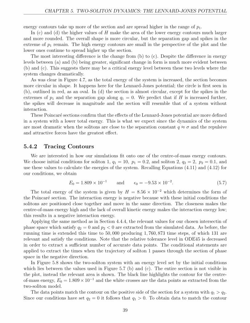
CHAPTER 5. TWO-SOLITON DYNAMICS: THE LENNARD-JONES POTENTIAL
energy contours take up more of the section and are spread higher in the range of p1.In (c) and (d) the higher values of H make the area of the lower energy contours much larger
and more rounded. The overall shape is more circular, but the separation gap and spikes in theextreme of p1 remain. The high energy contours are small in the perspective of the plot and thelower ones continue to spread higher up the section.
The most interesting difference is the change from (b) to (c). Despite the difference in energylevels between (a) and (b) being greater, significant change in form is much more evident between(b) and (c). This suggests there may be a critical energy level between these two levels where thesystem changes dramatically.
As was clear in Figure 4.7, as the total energy of the system is increased, the section becomesmore circular in shape. It happens here for the Lennard-Jones potential; the circle is first seen in(b), outlined in red, as an oval. In (d) the section is almost circular, except for the spikes in theextremes of p1 and the separation gap along q1 = 0. We predict that if H is increased further,the spikes will decrease in magnitude and the section will resemble that of a system withoutinteraction.
These Poincare sections confirm that the effects of the Lennard-Jones potential are more definedin a system with a lower total energy. This is what we expect since the dynamics of the systemare most dramatic when the solitons are close to the separation constant q ≈ σ and the repulsiveand attractive forces have the greatest effect.
5.4.2 Tracing Contours
We are interested in how our simulations fit onto one of the centre-of-mass energy contours.We choose initial conditions for soliton 1, q1 = 10, p1 = 0.2, and soliton 2, q2 = 2, p2 = 0.1, anduse these values to calculate the energies of the system. Recalling Equations (4.11) and (4.12) forour conditions, we obtain
E0 = 1.809× 10⁻¹ and ε0 = −9.53× 10⁻². (5.7)
The total energy of the system is given by H = 8.56 × 10⁻² which determines the form ofthe Poincare section. The interaction energy is negative because with these initial conditions thesolitons are positioned close together and move in the same direction. The closeness makes thecentre-of-mass energy high and the lack of overall kinetic energy makes the interaction energy low;this results in a negative interaction energy.
Applying the same method as in Section 4.4.4, the relevant values for our chosen intersectin ofphase space which satisfy q2 = 0 and p2 < 0 are extracted from the simulated data. As before, therunning time is extended this time to 50, 000 producing 1, 760, 873 time steps, of which 131 arerelevant and satisfy the conditions. Note that the relative tolerance level in ODE45 is decreasedin order to extract a sufficient number of accurate data points. The conditional statements areapplied to extract the times when the trajectory of soliton 1 passes through the section of phasespace in the negative direction.
In Figure 5.8 shows the two-soliton system with an energy level set by the initial conditionswhich lies between the values used in Figure 5.7 (b) and (c). The entire section is not visible inthe plot, instead the relevant area is shown. The black line highlights the contour for the centre-of-mass energy, E0 = 1.809× 10⁻¹ and the white crosses are the data points as extracted from thetwo-soliton model.
The data points match the contour on the positive side of the section for a system with q1 > q2.Since our conditions have set q2 = 0 it follows that q1 > 0. To obtain data to match the contour
39

CHAPTER 5. TWO-SOLITON DYNAMICS: THE LENNARD-JONES POTENTIAL
Figure 5.8: Poincare section for the two-soliton system with the Lennard-Jones potential for H =8.56 × 10⁻² given by initial conditions q1(0) = 10, p1(0) = 0.2, q2(0) = 2, p2(0) = 0.1. Simulated datapoints are overlaid in white and follow the black contour.
for the negative side the initial conditions should be altered such that q1 < q2. It is not possibleto have data points to appear for both sections from the same two-soliton model as the solitonsnever cross. The points fill the majority of the contour; an extended timescale would fill the wholecontour. The points do not lie cleanly on the contour even though the tolerance level has beenreduced. It is likely that if the timescale is increased the tolerance should be reduced again.
The contours shown in the Poincare sections for the Lennard-Jones potential are split, unlikethose for the interaction potential. The centre-of-mass energy level highlighted in Figure 5.8 isdisjointed with two contours appearing; a main one following the general form of the section andan additional contour at the top with p1 ≈ 0.5. This differs from the complete form of the contourson the sections for the interaction potential.
In this chapter we have analysed a two-soliton system which considers the Lennard-Jones po-tential. Having adapted Hamilton’s equations we examined the short term effects of the potential,observing the repulsion and attraction when the separation of the solitons is q ≈ σ, and foundthe frequency of the potential at this point. Extending the simulations we considered the effectsof adding the harmonic trap and varying the initial separation. Poincare sections allowed us toconsider similar systems with different energy levels. This proved important as the form of thesections was unusual and we gained better understanding for choosing suitable conditions for thesystem. Throughout we have compared these results to those obtained in Chapter 4.
40

Chapter 6
Summary
In this dissertation we introduced the concept of solitons and Bose-Einstein condensates anddiscussed how these can be used to model nonlinear systems. We considered the Gross-Pitaevskiiequation, examined the time-independent form and derived a soliton solution for one dimension.Whilst full computational modelling of the GPE could have been used, we applied Hamiltonianmechanics to systems which considered the soliton as a particle. We modelled a single soliton in aharmonic trap and observed simple harmonic motion as expected, validating the MATLAB model.Following the work by Marchant et al. [18], we introduced a barrier into the trap, examined thedynamics as the barrier height was varied, and found good agreement with the experimental data.Introducing a second soliton, we looked at systems which accounted for the interaction potentialand the Lennard-Jones potential separately. The classic interaction potential caused the phaseshift to occur when the solitons collided with sufficiently low momenta. We compared the effectsof the interaction potential frequency with the trap frequency by varying the initial separation.In the Lennard-Jones potential system, we observed the solitons repel when in close proximity.We found the frequency of the Lennard-Jones potential and compared its effects with the trapfrequency. In both systems we used Poincare sections to enable further understanding of themotion of the two solitons. The sections illustrated all possible trajectories and provided muchmore information than that offered from individual simulations.
As an extension to this dissertation, two-soliton systems which take into account both theLennard-Jones and the interaction potentials could be considered. The relative strengths of thepotentials are unknown and it would be interesting to see how this would affect the dynamicsof the solitons. Increasing the number of solitons in the system would complicate the dynamics;chaotic dynamics in a three-soliton system have been observed by Martin et al. [19] and it wouldbe interesting to consider a the Lennard-Jones potential in a three-soliton system.
41

References
[1] Russell J. Report on waves: made to the meetings of the British Association in 1842-43. 1845.
[2] Russell J, Robison J. Report of the Committee on Waves: appointed by the British Associationat Bristol in 1836.
[3] Drazin PG, Johnson RS. Solitons: An Introduction, vol. 2. Cambridge University Press, 1989.
[4] Lonngren K, Scott A. Solitons in Action. Academic Press Inc: New York, 1978.
[5] Zabusky NJ, Kruskal MD. Interaction of solitons in a collisionless plasma and the recurrenceof initial states. Phys. Rev. Lett 1965; 15(6):240–243.
[6] Korteweg D, De Vries G. On the change of form of long waves advancing in a rectangularcanal, and on a new type of long stationary waves. The London, Edinburgh, and DublinPhilosophical Magazine and Journal of Science 1895; 39(240):422–443.
[7] Hasegawa A, Tappert F. Transmission of stationary nonlinear optical pulses in dispersivedielectric fibers. I. Anomalous dispersion. Applied Physics Letters 2003; 23(3):142–144.
[8] Hasegawa A, Tappert F. Transmission of stationary nonlinear optical pulses in dispersivedielectric fibers. II. Normal dispersion. Applied Physics Letters 2003; 23(4):171–172.
[9] Commission on Physical Sciences M, Mathematics P, Council N, Board N, Sciences D. Non-linear Science. Compass series.
[10] Heisenberg W. Uber den anschaulichen inhalt der quantentheoretischen kinematik undmechanik. Zeitschrift fur Physik 1927; 43(3-4):172–198.
[11] Cornell E. Very cold indeed: The nanokelvin physics of Bose-Einstein condensation. NationalInstitute of Standards and Technology, Journal of Research 1996; 101(4):419–434.
[12] Einstein A. Quantentheorie des einatomigen idealen gases. 2. Sitzungsberichte der PreußischenAkademie der Wissenschaften 1925; .
[13] Anderson MH, Ensher JR, Matthews MR, Wieman CE, Cornell EA. Observation of Bose-Einstein condensation in a dilute atomic vapor. Science 1995; 269(5221):198–201.
[14] Ketterle W, Durfee D, Stamper-Kurn D. Making, probing and understanding Bose-Einsteincondensates. arXiv preprint cond-mat/9904034 1999; 5.
[15] Billam T, Marchant A, Cornish S, Gardiner S, Parker N. Bright solitary matter waves: forma-tion, stability and interactions. Spontaneous Symmetry Breaking, Self-Trapping, and Joseph-son Oscillations. Springer, 2013; 403–455.
42

REFERENCES
[16] Khaykovich L, Schreck F, Ferrari G, Bourdel T, Cubizolles J, Carr LD, Castin Y, SalomonC. Formation of a matter-wave bright soliton. Science 2002; 296(5571):1290–1293.
[17] Strecker KE, Partridge GB, Truscott AG, Hulet RG. Formation and propagation of matter-wave soliton trains. Nature 2002; 417(6885):150–153.
[18] Marchant A, Billam T, Wiles T, Yu M, Gardiner S, Cornish S. Controlled formation andreflection of a bright solitary matter-wave. Nature communications 2013; 4:1865.
[19] Martin A, Adams C, Gardiner S. Bright solitary-matter-wave collisions in a harmonic trap:Regimes of solitonlike behavior. Phys. Rev. A ; 77(1).
[20] Gross E. Unified Theory of Interacting Bosons. Phys. Rev. 1957; 106:161.
[21] Ginzburg V, Pitaevskii L. On the Theory of Superfluidity. Sov. Phys. JETP 1958; 7:858.
[22] Martin A. Theoretical Studies of Bright Solitons in Trapped Atomic Bose-Einstein Conden-sates. PhD Thesis, Durham University 2008.
[23] Parker N. Quantum Gases. MAS8114: Topics In Modern Applied Mathematics 2012/13.
[24] Gignoux C, Silvestre-Brac B. Solved problems in Lagrangian and Hamiltonian mechanics.Springer, 2009.
[25] Maki J, Kodama T. Phenomenological quantization scheme in a nonlinear Schrodinger equa-tion. Phys. Rev. Lett. 1986; 57(17):2097.
[26] Rafat M, Wheatland M, Bedding T. Dynamics of a double pendulum with distributed mass.American Journal of Physics 2009; 77(3):216–223.
[27] Korsch HJ, Jodl HJ, Hartmann T. Chaos: a program collection for the PC. Springer Publish-ing Company, Incorporated, 2008.
[28] Atkins P, de Paula J, Friedman R. Physical Chemistry: Quanta, Matter, and Change.
43