The Islamic University of GazaDeanery of Graduate StudiesFaculty of EngineeringElectrical Engineering Department

PARAMETERS IDENTIFICATION OFA PERMANENT MAGNET DC MOTOR

By

Mohammed S. Z. Salah

Supervisor

Prof. Dr. Muhammed Abdelati

“A Thesis Submitted in Partial Fulfillment of the Requirements for the

Degree of Master of Science in Electrical Engineering.”

1430 - 2009

Abstract

In this thesis, driver circuits to drive DC motor are designed and built. We take inour design the safety for any damage, the isolation from any interference and the ca-pability to provide the sufficient current needed to drive the motor. Also, methodsand algorithms used for parameters identification are addressed. Data acquisitionmodule form National Instruments is a suitable module used for acquiring signalssince it’s compatible with MATLAB and LABVIEW. To identify the parametersof the motor, an experimental measurement of armature voltage, armature currentand rotor speed are performed using the NIDAQ USB-6008 data acquisition mod-ule. Trials are performed to apply some of the methods on the motor practicallyto identify the motor parameters. DAQ toolbox in MATLAB/Simulink is used toacquire the test signals and perform analysis based on the nonlinear least squaremethod or pattern search method which they are suitable. Finally, we designed aGUI to be user friendly and to automate all the process of identification, in addi-tion to the feature for undergraduate and graduate students to apply experimentson control and machine labs. The extracted motor parameters from simulationproduced consistent simulation results with experimental data. The proposed ap-proaches are compared and both are proved to be simple, fast and accurate.

ii

: عنوان البحث بالعرب"ة

استخالb المچعامال^ الخاصة بالمچحرHg B الت"ا9 المچستمچر ”“

بع"ن األخذ تم ح"ث الد9اسة، في المچستخدم Bللمچحر التشغ"ل HIائر Hبناء تصمچ"م تم البحث هذا فيالالزم الت"ا9 تزOHد على القـد9ة Hكذلك مغناW"سـي تداخل Hأ Oحـدث Wا9ىء ألي األمان Hسـائل التصمچ"م في اإلعتبا9المچحـركا^، من النو_ بـ`ذا الخاصة المچعامال^ bاستخال في المچستخدمة cالطر 9Iاسة Hتم كمچا ، Bالمچحر لتشغ"ل

من الع"نا^ ملتقط fgهنمچو إستخدام تمHكذلك

الع"نا^ ملتقـط باسـتخدام Bالمچحر Hسرعةبـرهنامج

WرOقـة تطبـ"ق تم الن`اOة Hفي . 9Iاسـت`ا تم التي cالطر بـعض لتطب"قWرOقة

مععدة إضافة مع ، المچطلوبـة التحـل"ل"ة الرسـوما^ Hإo`ا9 المچعامال^ bإسـتخال عمچل"ة Oسـ`ل حـتىتم التي المچعامال^ Hاآلال^. التحــــــكم sمجا في التجا9ب بــــــعض تطبــــــ"ق من HالخرOج"ن الطالب تمچكن مزاOااإلفتراضي. Hالنظام الحق"قـــي النظام بــ"ن اإلستجابــة تطابــق في gلك Hتبــ"ن مقبــولة هنتائج أعطت اســتخالص`ابـــــ"ن`مچا. مقــــا9هنة عمچل تم حــــ"ث الدقــــة Hكذلك Hالســــرعة بالبســــاWة تتمچ"زان المچقترحــــتان الطرOقــــتان

المچباشر الت"ا9 Hg

National InstrumentsLABVIEW

NIDAQ USB-6008 )MATLAB

Nonlinear Least SquarePattern Search

MATLAB/SimulinkMATLAB

مع لتوافقه لإلستخدام لمچناسبتهHت"ا9 بــج`د الخاصة الع"نا^ ألخذ تطب"قــي هنظام بــناء تم المچعامال^ هذ| bالسـتخالH ،باسـتخدام الع"نا^ هذ| تحـل"ل Hتم كمچا . (محـاHال^ عدة إجراء تم . الع"نا^ ملتقـط مع الالزمة المچحـاكاة Hعمچل sبـاالتصا Oقـوم الذيHكذلكHالمچتوافقـة إOجاIها في المچناسبتان الطرOقتان ألهن`مچا المچعامال^ bاستخال عمچل"ة في

باستخدام محاكاة شاشة بتصمچ"م العمچل"ا^ هذ| جمچ"ع أتمچتة تم ،

MATLAB

GUIفي Iالمچوجو

iii

Dedication

To my family members who have been a constant source of

motivation, inspiration, and support.

iv

Acknowledgements

I would like to thank my thesis supervisor, Prof. Dr. Muhammed Abdelati, for hissupport, encouragement and professional assistance.

Special thanks to all other Islamic University staff members that I may have calledupon for assistance especially Dr. Iyad Abu-Hudrouss and Dr. Mohammed Alhan-jouri, as their suggestions have helped with the development of this thesis.

I would also like to extend my gratitude to my family for the support they havegiven me. Also my thanks to my friends for the precious opportunity they gave meto study in.

v

Contents

Abstract ii

Dedication iv

Acknowledgements v

List of Tables viii

List of Figures ix

List of Nomenclatures xi

List of Abbreviations xii

1 Introduction and Literature Review 11.1 Research Motivation and Goal . . . . . . . . . . . . . . . . . . . . . 11.2 Literature Review . . . . . . . . . . . . . . . . . . . . . . . . . . . . 11.3 Methodology . . . . . . . . . . . . . . . . . . . . . . . . . . . . . . 51.4 The Identification Process . . . . . . . . . . . . . . . . . . . . . . . 6

1.4.1 Collecting Information about the System . . . . . . . . . . . 71.4.2 Selecting a Model Structure to Represent the System . . . . 71.4.3 Matching the Selected Model Structure

to the Measurements . . . . . . . . . . . . . . . . . . . . . . 91.4.4 Validating the Selected Model . . . . . . . . . . . . . . . . . 9

1.5 Thesis Structure . . . . . . . . . . . . . . . . . . . . . . . . . . . . . 9

2 DC Motors and Parameters Identification 102.1 History and Background . . . . . . . . . . . . . . . . . . . . . . . . 102.2 Categorization of Electric Motors . . . . . . . . . . . . . . . . . . . 112.3 DC Motors . . . . . . . . . . . . . . . . . . . . . . . . . . . . . . . 11

2.3.1 Brushed DC motors . . . . . . . . . . . . . . . . . . . . . . . 122.4 Principle of Operation . . . . . . . . . . . . . . . . . . . . . . . . . 13

2.4.1 Production of Torque . . . . . . . . . . . . . . . . . . . . . . 132.4.2 Generated E.M.F. . . . . . . . . . . . . . . . . . . . . . . . . 162.4.3 Motor Modeling and Simulation . . . . . . . . . . . . . . . . 17

2.5 Parameters Identification . . . . . . . . . . . . . . . . . . . . . . . . 192.5.1 Pseudo Inverse Technique . . . . . . . . . . . . . . . . . . . 19

vi

2.5.2 Nonlinear Least-Square Method . . . . . . . . . . . . . . . . 222.5.3 Pattern Search Algorithm . . . . . . . . . . . . . . . . . . . 23

3 System Hardware Development 263.1 Introduction . . . . . . . . . . . . . . . . . . . . . . . . . . . . . . . 263.2 Hardware Design . . . . . . . . . . . . . . . . . . . . . . . . . . . . 273.3 The MOSFET as a Switch . . . . . . . . . . . . . . . . . . . . . . . 28

3.3.1 Introduction . . . . . . . . . . . . . . . . . . . . . . . . . . . 283.3.2 Choosing a MOSFET . . . . . . . . . . . . . . . . . . . . . . 293.3.3 MOSFET Gate Driver . . . . . . . . . . . . . . . . . . . . . 31

3.4 Pulse Width Modulation (PWM) . . . . . . . . . . . . . . . . . . . 323.5 Power Supply . . . . . . . . . . . . . . . . . . . . . . . . . . . . . . 343.6 Voltage Doubler . . . . . . . . . . . . . . . . . . . . . . . . . . . . . 353.7 Sensors and Feedback Elements . . . . . . . . . . . . . . . . . . . . 35

3.7.1 Introduction . . . . . . . . . . . . . . . . . . . . . . . . . . . 353.7.2 Current Sensors . . . . . . . . . . . . . . . . . . . . . . . . . 363.7.3 Shunt Resistors as a Current Sensor . . . . . . . . . . . . . . 373.7.4 Speed/Position Sensor . . . . . . . . . . . . . . . . . . . . . 383.7.5 Voltage Sensing . . . . . . . . . . . . . . . . . . . . . . . . . 39

4 Experimentation, Testing and Results 404.1 Experimental System . . . . . . . . . . . . . . . . . . . . . . . . . . 404.2 DC Motor Speed . . . . . . . . . . . . . . . . . . . . . . . . . . . . 414.3 Panel Meters . . . . . . . . . . . . . . . . . . . . . . . . . . . . . . 424.4 Sensing Circuit . . . . . . . . . . . . . . . . . . . . . . . . . . . . . 434.5 Interfacing Circuit . . . . . . . . . . . . . . . . . . . . . . . . . . . 444.6 Data Acquisition . . . . . . . . . . . . . . . . . . . . . . . . . . . . 454.7 Parameters Identification . . . . . . . . . . . . . . . . . . . . . . . . 46

4.7.1 GUI Interface . . . . . . . . . . . . . . . . . . . . . . . . . . 55

5 Conclusions and Future Work 605.1 Conclusions . . . . . . . . . . . . . . . . . . . . . . . . . . . . . . . 605.2 Future Work . . . . . . . . . . . . . . . . . . . . . . . . . . . . . . . 605.3 Summary of Contributions . . . . . . . . . . . . . . . . . . . . . . . 61

Bibliography 63

A MALTLAB Codes 66A.1 Acquiring Signals . . . . . . . . . . . . . . . . . . . . . . . . . . . . 66A.2 Parameters Identification . . . . . . . . . . . . . . . . . . . . . . . . 71A.3 Validation of Identification . . . . . . . . . . . . . . . . . . . . . . . 73

B Schematics 75

vii

List of Tables

2.1 DC motor parameters. . . . . . . . . . . . . . . . . . . . . . . . . . 20

3.1 Specification of experimental dc motor. . . . . . . . . . . . . . . . . 263.2 MOSFET Drivers. . . . . . . . . . . . . . . . . . . . . . . . . . . . 313.3 Current sensing methods. . . . . . . . . . . . . . . . . . . . . . . . 37

4.1 Interfacing circuit DB9 pinout . . . . . . . . . . . . . . . . . . . . . 444.2 NI DAQ inputs and outputs. . . . . . . . . . . . . . . . . . . . . . . 464.3 Summary of parameter estimation process(NLS method) . . . . . . 574.4 Summary of parameter estimation results(NLS method) . . . . . . . 574.5 Summary of parameter estimation process(Pattern method) . . . . 574.6 Summary of parameter estimation results(Pattern method) . . . . . 58

5.1 Parameter estimation results . . . . . . . . . . . . . . . . . . . . . . 62

viii

List of Figures

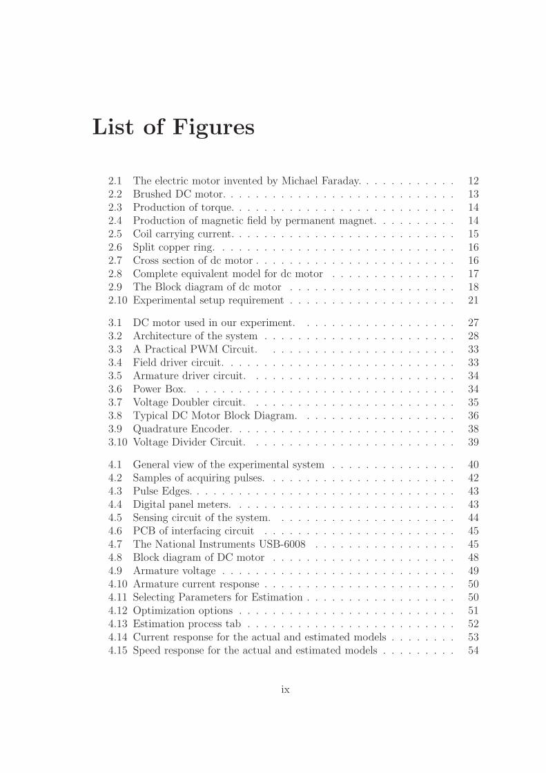
2.1 The electric motor invented by Michael Faraday. . . . . . . . . . . . 122.2 Brushed DC motor. . . . . . . . . . . . . . . . . . . . . . . . . . . . 132.3 Production of torque. . . . . . . . . . . . . . . . . . . . . . . . . . . 142.4 Production of magnetic field by permanent magnet. . . . . . . . . . 142.5 Coil carrying current. . . . . . . . . . . . . . . . . . . . . . . . . . . 152.6 Split copper ring. . . . . . . . . . . . . . . . . . . . . . . . . . . . . 162.7 Cross section of dc motor . . . . . . . . . . . . . . . . . . . . . . . . 162.8 Complete equivalent model for dc motor . . . . . . . . . . . . . . . 172.9 The Block diagram of dc motor . . . . . . . . . . . . . . . . . . . . 182.10 Experimental setup requirement . . . . . . . . . . . . . . . . . . . . 21

3.1 DC motor used in our experiment. . . . . . . . . . . . . . . . . . . 273.2 Architecture of the system . . . . . . . . . . . . . . . . . . . . . . . 283.3 A Practical PWM Circuit. . . . . . . . . . . . . . . . . . . . . . . 333.4 Field driver circuit. . . . . . . . . . . . . . . . . . . . . . . . . . . . 333.5 Armature driver circuit. . . . . . . . . . . . . . . . . . . . . . . . . 343.6 Power Box. . . . . . . . . . . . . . . . . . . . . . . . . . . . . . . . 343.7 Voltage Doubler circuit. . . . . . . . . . . . . . . . . . . . . . . . . 353.8 Typical DC Motor Block Diagram. . . . . . . . . . . . . . . . . . . 363.9 Quadrature Encoder. . . . . . . . . . . . . . . . . . . . . . . . . . . 383.10 Voltage Divider Circuit. . . . . . . . . . . . . . . . . . . . . . . . . 39

4.1 General view of the experimental system . . . . . . . . . . . . . . . 404.2 Samples of acquiring pulses. . . . . . . . . . . . . . . . . . . . . . . 424.3 Pulse Edges. . . . . . . . . . . . . . . . . . . . . . . . . . . . . . . . 434.4 Digital panel meters. . . . . . . . . . . . . . . . . . . . . . . . . . . 434.5 Sensing circuit of the system. . . . . . . . . . . . . . . . . . . . . . 444.6 PCB of interfacing circuit . . . . . . . . . . . . . . . . . . . . . . . 454.7 The National Instruments USB-6008 . . . . . . . . . . . . . . . . . 454.8 Block diagram of DC motor . . . . . . . . . . . . . . . . . . . . . . 484.9 Armature voltage . . . . . . . . . . . . . . . . . . . . . . . . . . . . 494.10 Armature current response . . . . . . . . . . . . . . . . . . . . . . . 504.11 Selecting Parameters for Estimation . . . . . . . . . . . . . . . . . . 504.12 Optimization options . . . . . . . . . . . . . . . . . . . . . . . . . . 514.13 Estimation process tab . . . . . . . . . . . . . . . . . . . . . . . . . 524.14 Current response for the actual and estimated models . . . . . . . . 534.15 Speed response for the actual and estimated models . . . . . . . . . 54

ix

4.16 Trajectories of estimated parameters . . . . . . . . . . . . . . . . . 554.17 Parameters estimation results . . . . . . . . . . . . . . . . . . . . . 564.18 Current response for the actual and estimated models . . . . . . . . 584.19 Speed response for the actual and estimated models . . . . . . . . . 584.20 GUI interface . . . . . . . . . . . . . . . . . . . . . . . . . . . . . . 59

B.1 Field driver unit schematics. . . . . . . . . . . . . . . . . . . . . . 76B.2 Field driver unit layout. . . . . . . . . . . . . . . . . . . . . . . . . 77B.3 Armature driver unit. . . . . . . . . . . . . . . . . . . . . . . . . . 78B.4 Armature driver unit layout. . . . . . . . . . . . . . . . . . . . . . 79B.5 Armature power circuit. . . . . . . . . . . . . . . . . . . . . . . . . 80B.6 Field power circuit. . . . . . . . . . . . . . . . . . . . . . . . . . . 81B.7 interfacing circuit. . . . . . . . . . . . . . . . . . . . . . . . . . . . 82

x

List of Nomenclatures

I Current.B Magnetic field flux density.F Force.l Length of wire.T Torque.N Number of turns.Tm Motor’s torque.Kt Motor’s torque constant.e Electromotive force.λ Flux linking the coil.θm Angle between the pole-faces.φ Magnetic flux linking the coil.ωm Constant angular speed.Ke Back-EMF constant.Kt Torque constant.Ra Terminal resistance.La Armature inductance.J Moment of inertia of the rotor.B Viscous (damping) friction.s Laplace domain.z Z-transform domain.W Rotor speed.V Armature voltage.RDS Drain to source MOSFET resistance.

xi

List of Abbreviations

AC Alternative Current.AI Analog Input.AO Analog Output.CPR Counts Per Revolution.DAQ Data Acquisition.DAT Data Acquisition Toolbox.DC Direct Current.DSP Digital Signal Processing.EMF Electromotive Force.EMI Electromagnetic Interference.FET Field Effect Transistor.FPGA Field Programmable Gate Array.GUI Graphical User Interface.GPS Generalized Pattern Search Algorithm.IC Integrated Circuit.IOS Input Current Offset.LED Light Emitting Diode.MADS Mesh Adaptive Search Algorithm.MCU Microcontroller Unit.MOSFET Metal Oxide Semiconductor Field Effect Transistor.NI National Instruments.PCB Printed Circuit Board.PC Personal Computer.PD Proportional Derivative.PIC Programmable Interface Controller.PWM Pulse Width Modulation.USB Universal Serial Bus.VOS Voltage Offset.

xii

Chapter 1

Introduction and LiteratureReview

1.1 Research Motivation and Goal

In practical life and through building projects, we depend widely on using DCmotors as the main component for producing motion and torque. These motorsare taken from electronic devices such as printers, imaging machines, scanners andother old devices. The problem we face is that these motors does not have anyindustrial information. These information are the parameters which describe themathematical model of motor to use it in simulation softwares such as MATLABand LABVIEW. The mathematical model help predicting system behavior anddesigning system controller. Because we haven’t the parameters of motor, we face aproblem of implementing it or to precise control it. In our thesis we build the driversand use a data acquisition module and MATLAB to estimate these parameters usingnonlinear least square method. This method is an accurate method for estimationparameters by iterative procedure.

The goals for parameters identification are implementing an accurate mathe-matical models, design precise controllers, predict the closed loop behavior of theplant, researches validate manufacture supplied parameters and specify missing in-formation.

1.2 Literature Review

We studied the modeling of dc motors for control applications [1], and we foundthat there are three different mathematical models of an armature controlled dcmotors. These models are:

1. Precise nonlinear model.

2. Piecewise linear model.

1

3. Second-order linear model.

A mathematical model for a physical device must often reflect a compromise. Itmust not attempt to mirror the real device in such great detail that the model be-comes cumbersome; on the other hand it should not be so simplified that predictionsand explanations based on it are either trivial or far from reality.

In our thesis we used the second order linear model over other models due toits simplicity. The main difficulty with the nonlinear models is the requirement ofnumerical solution and the use of this model in those applications of adaptive andoptimal control which require a digital computer. The second-order linear modelassumes the following for ease of use:

1. The static friction is negligible and the frictional torque can be considereddirectly proportional to angular velocity.

2. The brush voltage drop is negligible.

3. Armature reaction can be neglected.

4. The resistance and the inductance of the armature can be regarded as con-stant.

We noticed from modeling that there is a variation of the inductance of the armaturewith armature current, so convential methods for dc motor parameters identificationis not accurate and lead to poor controlling.

Accurate mathematical models and their parameters are essential when design-ing controllers because they allow the designer to predict the closed loop behavior ofthe plant. Errors in parameter values can lead to poor control and instability. Theconvential way of characterizing a dc motor is to perform a separate test for eachparameter, but this is not only time consuming, but can yield misleading results ifthe parameters are measured under static or no load conditions. Therefore, esti-mation techniques must be used to estimate the unknown or inaccurate parametersvalues with precision. Estimation approaches can be divided into two categories:offline estimation and online estimation.

Offline techniques use specific test inputs, measure the corresponding outputsignals and then try to establish the relation between them. Online techniquesuse, for example, observers and Kalman filters to recursively estimate parameters.Neural networks can be used in either offline or online approaches.

There are many techniques and ordered from old to new, each technique hasits own method for parameters identification. Each technique has advantages overthe other and some have some disadvantages. The following techniques are listedbelow:

In 1973, W. Lord and J. H. Hwang identified eight practical servomotor modelsfor separately excited dc servomotors, and the parameters of each model are clearly

2

defined. Testing procedures are given for determining a servomotor’s model typeand all the model parameters based only on the current response of the machineto a step input of armature voltage. Excellent agreement is obtained betweenthe actual current responses of several servomotors and their predicted responsesobtained from the corresponding mathematical models, indicating the efficacy ofthe technique [2].

In 1975, W. Lord and J. H. Hwang showed that linear modeling techniques areapplicable to separately excited dc motors if the model parameters are obtainedunder dynamic operating conditions. They used Pasek’s technique in order toidentify the model type and all the model parameters from single current responseof the motor to a step input of armature voltage [3].

In 1983, R. Schulz introduced a frequency response technique for measuring theparameters of high-performance dc motors. A second-order motor model, undercertain conditions, is shown to be equivalent to a series resonant electrical cir-cuit. Frequency response measurements of the motor, when treated as electricalimpedance, form the basis of a measurement technique which has certain practi-cal advantages. Results are compared to measurements made using conventionalmethods [4].

In 1988, A. D. Rajkumar and R. Somanatham proposed practical determina-tion of direct current (dc) motor transients is generally possible only by usingsophisticated transient recorders or storage oscilloscopes. In this paper a methodis presented to determine dc motor transients using an 8085 based microcomputer.The scheme was tested in the laboratory and results verified [5].

In 1991, S. Weerasooriya and M. A. El-Sharkawi introduced and artificial neuralnetwork based high performance speed control system for a dc motor. The purposeis to achieve accurate trajectory control of the speed, specially when motor and loadparameters are unknown. The unknown nonlinear dynamics of the motor and theload are captured by an artificial neural network. Performance of the identificationand control algorithms are evaluated by simulating them on a typical dc motormodel [6].

In 1992, Y. Jung, K. Cho, Y. Lim, J. Park and Y. Chang described effortsto develop a microcomputer-based parameter identification system for a brushlessDC motor (BDCM). A BDCM is equal to a DC motor in the equivalent circuit.Therefore, Pasek’s equation for the parameter determination of a DC motor isapplicable to a BDCM. A new identification algorithm for BDCM parameters usingPasek’s technique is developed. The algorithm is implemented on an IBM-PC/ATusing the C language [7].

In 1996, D. M. Gillard and K. E. Bollinger described an investigation into theuse of a multilayered neural network for measuring the transfer function of a powersystem for use in power system stabilizer (PSS) tuning and assessing PSS damping.The objectives are to quickly and accurately measure the transfer function relatingthe electric power output to the AVR PSS reference voltage input of a system with

3

the plant operating under normal conditions In addition, the excitation signal usedin the identification procedure is such that it will not adversely affect the terminalvoltage or the system frequency [8].

In 2000 A. Rubbai and R. Kotaru proposed online identification and controlof dc motor using learning adaptation. Use is made of the power of feedforwardartificial neural networks to capture and emulate detailed nonlinear mappings, inorder to implement a full nonlinear control law [9].

In 2000 X. Liu, H. Zhang, J. Liu and J. Yang described Parameter estimationbased on block-pulse function series to estimate the continuous-time model of themotor. The electromechanical parameters of the motor can be obtained from theestimated model parameters [10].

In 2001, S. Saab and R. Abi Kaed-Bey showed that the parameters of a dcmotor can be estimated experimentally by employing discrete measurements of anintegrated dynamometer. The dynamometer outputs are the discrete measurementsof the armature current, angular velocity, armature voltage (system input), andthe torque developed by the motor. They employed least-squares algorithm toimplement the parameter identification of dc motor without the use of a D/Aconverter and a power amplifier. A Kalman filter is also implemented, as a stateobserver, to estimate the angular acceleration and the derivative of the armaturecurrent. In addition, to improve the overall identification performance, the DCparameters were first estimated by decoupling the AC parameters using a DC inputsignal [11].

In 2004, A. Dupuis, M. Ghribi and A. Kaddouri simplified the offline identifica-tion of motor parameters by proposing a new method based on optimization usinga multiobjective elitist genetic algorithm. The non-dominated sorting genetic algo-rithm (NSGA-11) is used to minimize the error between the current and velocityresponses of data and an estimated model. The robustness of the method is shownby estimating parameters of a DC motor in four different cases. Simulation re-sults show that the method successfully estimates the motor parameters and is alsocapable of identifying a load torque simultaneously [12].

In 2005, R. Krneta, S. Antic, and D. Stojanovic investigated the issues involvedin applying recursive least squares method in parameters identification of DC motormodels. The validity of the proposed method was shown by simulation an exper-iments. By comparing a graphic of real motor speed and a graphics of speed ofinvestigated models in a Z and S domains it can be concluded that a satisfyingquality of DC motor parameters identification has been achieved [13].

In 2006, R. Garrido and R. Miranda proposed a new method for closed loopidentification of position controlled dc servomechanisms. The loop around the servois closed using a Proportional Derivative (PD) controller. A model of the servo issimultaneously controlled using a second PD controller. The error and its timederivative between the output of both, the real servo and its model, is employedfor identifying the motor parameters which in turn are employed for updating the

4

model. Properties of the identification scheme are studied using Lyapunov stabilitytheory [14].

In 2007, W. Aung described the analysis on modeling and simulink of DC motorand its driving system, hardware and software. For DC Motor Modeling, it can beanalyzed with control techniques of Step response, Impulse response and Bode plotby using MATLAB Simulink. All data based on the internal circuit of a simple DCMotor and its features can be analyzed both by Control System design calculationand by MATLAB software [15].

In 2009, M. Hadef and M. Rachid described a parameter identification methodusing inverse problem methodology is proposed. The minimization of the objectivefunction with respect to the desired vector of design parameters is the most impor-tant procedure in solving the inverse problem. The conjugate gradient method isused to determine the unknown parameters, and Tikhonovs regularization methodis then used to replace the original ill-posed problem with a well-posed problem [16].

1.3 Methodology

In this thesis, we made a study on different identification methods were used in orderto get accurate parameters of dc motor compatible to our experimental model.

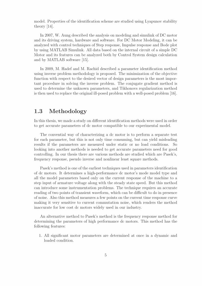
The convential way of characterizing a dc motor is to perform a separate testfor each parameter, but this is not only time consuming, but can yield misleadingresults if the parameters are measured under static or no load conditions. Solooking into another methods is needed to get accurate parameters need for goodcontrolling. In our thesis there are various methods are studied which are Pasek’s,frequency response, pseudo inverse and nonlinear least square methods.

Pasek’s method is one of the earliest techniques used in parameters identificationof dc motors. It determines a high-performance dc motor’s mode model type andall the model parameters based only on the current response of the machine to astep input of armature voltage along with the steady state speed. But this methodcan introduce some instrumentation problems. The technique requires an accuratereading of two points of transient waveform, which can be difficult to do in presenceof noise. Also this method measures a few points on the current time response curvemaking it very sensitive to current commutation noise, which renders the methodinaccurate for low cost dc motors widely used in our industry.

An alternative method to Pasek’s method is the frequency response method fordetermining the parameters of high performance dc motors. This method has thefollowing features:

1. All significant motor parameters are determined at once in a dynamic andloaded condition.

5

2. No nonelectrical measurements are required (such as speed in Pasek’s method).

3. Results are averaged out to minimize errors caused by noise.

4. Sophisticated instrumentation is not necessary.

5. The approach is readily adaptable to automatic testing.

Frequency response method determines the parameters of high performance dcmotors by treating a second order motor model as an electrical impedance (RLCcircuit), and by tuning the values of RLC circuit elements to match the responseof dc motor and by some relations the parameters of dc motor are calculated. Thismethod uses an ac signal with specific frequency about 1kHz. Unfortunately, thismethod is not suitable to the power drivers used in our experimental platform.Sensitivity to noise is another reason that discouraged us to utilized this method.

The pseudo inverse technique is a method capable of identifying an equiva-lent discrete transfer function of simple systems like motor, thermal system, massdamper systems etc with no zeros (only poles). This method assumes a single inputsingle output system and unable to find the dc motor parameters and doesn’t fitour objective [16].

Nonlinear least square method is a general approach in identification seeks todefine an objective function that would reach its minimum. The physical systemto be investigated is described in terms of parameters, and then, the objectivefunction is minimized with respect to the parameters by an iterative procedure. Atthe minimum of the objective function, the values of the parameters describe thereal structure of the physical system [17].

Pattern search algorithm is another method used in this thesis and appliedpractically on our experimental system. Pattern search is an attractive alternativeto the genetic algorithm, as it is often computationally less expensive and canminimize the same types of functions. Finally, this method can be used to find themotor parameters with less error and compare it with previous methods.

1.4 The Identification Process

Each identification session consists of a series of basic steps. Some of them may behidden or selected without the user being aware of his choice [18]. Clearly, this canresult in poor or suboptimal results. In each session the following actions shouldbe taken:

• Collecting information about the system.

• Selecting a model structure to represent the system.

6

• Choosing the model parameters to fit the model as well as possible to themeasurements: selection of a ”goodness of fit” criterion.

• Validating the selected model.

Each of these points is discussed in more detail next.

1.4.1 Collecting Information about the System

If we want to build a model for a system, we should get information about it. Thiscan be done by just watching the natural fluctuations, but most often it is moreefficient to set up dedicated experiments that actively excite the system. In thelatter case, the user has to select an excitation that optimizes his own goal (forexample, minimum cost, minimum time, or minimum power consumption for agiven measurement accuracy) within the operator constraints. The quality of thefinal result can depend heavily on the choices that are made.

1.4.2 Selecting a Model Structure to Represent the System

A choice should be made within all the possible mathematical models that can beused to represent the system. Again a wide variety of possibilities exist, such as:

• Parametric versus nonparametric models:

In a parametric model, the system is described using a limited number ofcharacteristic quantities called the parameters of the model, whereas in anonparametric model the system is characterized by measurements of a sys-tem function at a large number of points. Examples of parametric modelsare the transfer function of a filter described by its poles and zeros and themotion equations of a piston. An example of a nonparametric model is thedescription of a filter by its impulse response at a large number of points.

Usually it is simpler to create a nonparametric model than a parametricone because the modeler needs less knowledge about the system itself in theformer case. However, physical insight and concentration of information aremore substantial for parametric models than for nonparametric ones.

• White box models versus black box models:

In the construction of a model, physical laws whose availability and appli-cability depend on the insight and skills of the experimenter can be used(Kirchhoff’s laws, Newton’s laws, etc.). Specialized knowledge related to dif-ferent scientific fields may be brought into this phase of the identificationprocess. The modeling of a loudspeaker, for example, requires extensive un-derstanding of mechanical, electrical, and acoustical phenomena. The resultmay be a physical model, based on comprehensive knowledge of the inter-nal functioning of the system. Such a model is called a white box model.Another approach is to extract a black box model from the data. Instead

7

of making a detailed study and developing a model based upon physical in-sight and knowledge, a mathematical model is proposed that allows sufficientdescription of any observed input and output measurements. This reducesthe modeling effort significantly. For example, instead of modeling the loud-speaker using physical laws, an input-output relation, taking the form of ahigh-order transfer function, could be proposed. The choice between the dif-ferent methods depends on the aim of the study: the white box approach isbetter for gaining insight into the working principles of a system, but a blackbox model may be sufficient if the model will be used only for prediction ofthe output. Although, as a rule of thumb, it is advisable to include as muchprior knowledge as possible during the modeling process, it is not always easyto do it. If we know, for example, that a system is stable, it is not simple toexpress this information if the polynomial coefficients are used as parameters.

• Linear models versus nonlinear models:

In real life, almost every system is nonlinear. Because the theory of nonlinearsystems is very involved, these are mostly approximated by linear models,assuming that in the operation region the behavior can be linearized. Thiskind of approximation makes it possible to use simple models without jeopar-dizing properties that are of importance to the modeler. This choice dependsstrongly on the intended use of the model. For example, a nonlinear modelis needed to describe the distortion of an amplifier, but a linear model willbe sufficient to represent its transfer characteristics if the linear behavior isdominant and is the only interest.

• Linear-in-the-parameters versus nonlinear-in-the-parameters:

A model is called linear-in-the-parameters if there exists a linear relationbetween these parameters and the error that is minimized. This does notimply that the system itself is linear. For example, ǫ = y − (a1u + a2u

2) islinear in the parameters a1 and a2 but describes a nonlinear system. On theother hand,

ǫ(jω) = Y (jω)−a0 + a1jω

b0 + b1jωU(jω) (1.1)

describes a linear system but the model is nonlinear in the b0 and b1 parame-ters. Linearity in the parameters is a very important aspect of models becauseit has a strong impact on the complexity of the estimators if a (weighted) leastsquares cost function is used. In that case, the problem can be solved ana-lytically for models that are linear in the parameters so that an iterativeoptimization problem is avoided.

8

1.4.3 Matching the Selected Model Structure

to the Measurements

Once a model structure is chosen (e.g., a parametric transfer function model), itshould be matched as well as possible with the available information about thesystem. Mostly, this is done by minimizing a criterion that measures a goodness ofthe fit. The choice of this criterion is extremely important because it determinesthe stochastic properties of the final estimator. Many choices are possible and eachof them can lead to a different estimator with its own properties. Usually, the costfunction defines a distance between the experimental data and the model. The costfunction can be chosen on an ad hoc basis using intuitive insight, but there alsoexists a more systematic approach based on stochastic arguments.

1.4.4 Validating the Selected Model

Finally, the validity of the selected model should be tested: does this model describethe available data properly or are there still indications that some of the dataare not well modeled, indicating remaining model errors? In practice, the bestmodel (= the smallest errors) is not always preferred. Often a simpler model thatdescribes the system within user-specified error bounds is preferred. Tools willbe provided that guide the user through this process by separating the remainingerrors into different classes, for example, unmodeled linear dynamics and nonlineardistortions. From this information, further improvements of the model can beproposed, if necessary. During the validation tests it is always important to keepthe application in mind. The model should be tested under the same conditionsas it will be used later. Extrapolation should be avoided as much as possible. Theapplication also determines what properties are critical.

Good understanding of the intended applications helps to set up good experi-ments, and is very important to make the proper simplifications during the model-building process.

1.5 Thesis Structure

There are five chapters in this thesis. Chapter 1 provides introduction and Litera-ture review. Chapter 2 concerns about dc motor principles and modeling. Chapter3 presents system hardware development. Chapter 4 provide experimental system,tests and results. Finally, in the last chapter conclusions and future work are given.

9

Chapter 2

DC Motors and ParametersIdentification

2.1 History and Background

An electric motor is a device using electrical energy to produce mechanical energy,nearly always by the interaction of magnetic fields and current-carrying conductors.The reverse process, that of using mechanical energy to produce electrical energy,is accomplished by a generator or dynamo. Traction motors used on vehicles oftenperform both tasks [19].

Electric motors are found in myriad uses such as industrial fans, blowers andpumps, machine tools, household appliances, power tools, and computer disk drives,among many other applications. Electric motors may be operated by direct currentfrom a battery in a portable device or motor vehicle, or from alternating currentfrom a central electrical distribution grid. The smallest motors may be found inelectric wristwatches. Medium-size motors of highly standardized dimensions andcharacteristics provide convenient mechanical power for industrial uses. The verylargest electric motors are used for propulsion of large ships, and for such purposesas pipeline compressors, with ratings in the thousands of kilowatts. Electric motorsmay be classified by the source of electric power, by their internal construction, andby application.

The physical principle of production of mechanical force by the interaction of anelectric current and a magnetic field was known as early as 1821. Electric motors ofincreasing efficiency were constructed throughout the 19th century, but commercialexploitation of electric motors on a large scale required efficient electrical generatorsand electrical distribution networks.

10

2.2 Categorization of Electric Motors

The classic division of electric motors has been that of Alternating Current (AC)types vs Direct Current (DC) types. This is more a de facto convention, ratherthan a rigid distinction. For example, many classic DC motors run on AC power,these motors being referred to as universal motors.

Rated output power is also used to categorize motors, those of less than 746Watts, for example, are often referred to as fractional horsepower motors (FHP) inreference to the old imperial measurement.

The ongoing trend toward electronic control further muddles the distinction,as modern drivers have moved the commutator out of the motor shell. For thisnew breed of motor, driver circuits are relied upon to generate sinusoidal AC drivecurrents, or some approximation of. The two best examples are: the brushless DCmotor and the stepping motor, both being poly-phase AC motors requiring externalelectronic control, although historically, stepping motors (such as for maritime andnaval gyrocompass repeaters) were driven from DC switched by contacts.

Considering all rotating (or linear) electric motors require synchronism betweena moving magnetic field and a moving current sheet for average torque production,there is a clearer distinction between an asynchronous motor and synchronous types.An asynchronous motor requires slip between the moving magnetic field and awinding set to induce current in the winding set by mutual inductance; the mostubiquitous example being the common AC induction motor which must slip inorder to generate torque. In the synchronous types, induction (or slip) is not arequisite for magnetic field or current production (eg. permanent magnet motors,synchronous brush-less wound-rotor doubly-fed electric machine).

2.3 DC Motors

A DC motor is designed to run on DC electric power. Two examples of pure DCdesigns are Michael Faraday’s homopolar motor (which is uncommon), and the ballbearing motor.

A homopolar motor has a magnetic field along the axis of rotation and anelectric current that at some point is not parallel to the magnetic field. The namehomopolar refers to the absence of polarity change. Homopolar motors necessarilyhave a single-turn coil, which limits them to very low voltages. This has restrictedthe practical application of this type of motor. Figure of this motor is shown inFigure 2.1.

A ball bearing motor is an unusual electric motor that consists of two ball-bearing-type bearings, with the inner races mounted on a common conductive shaft,and the outer races connected to a high current, low voltage power supply. Analternative construction fits the outer races inside a metal tube, while the inner

11

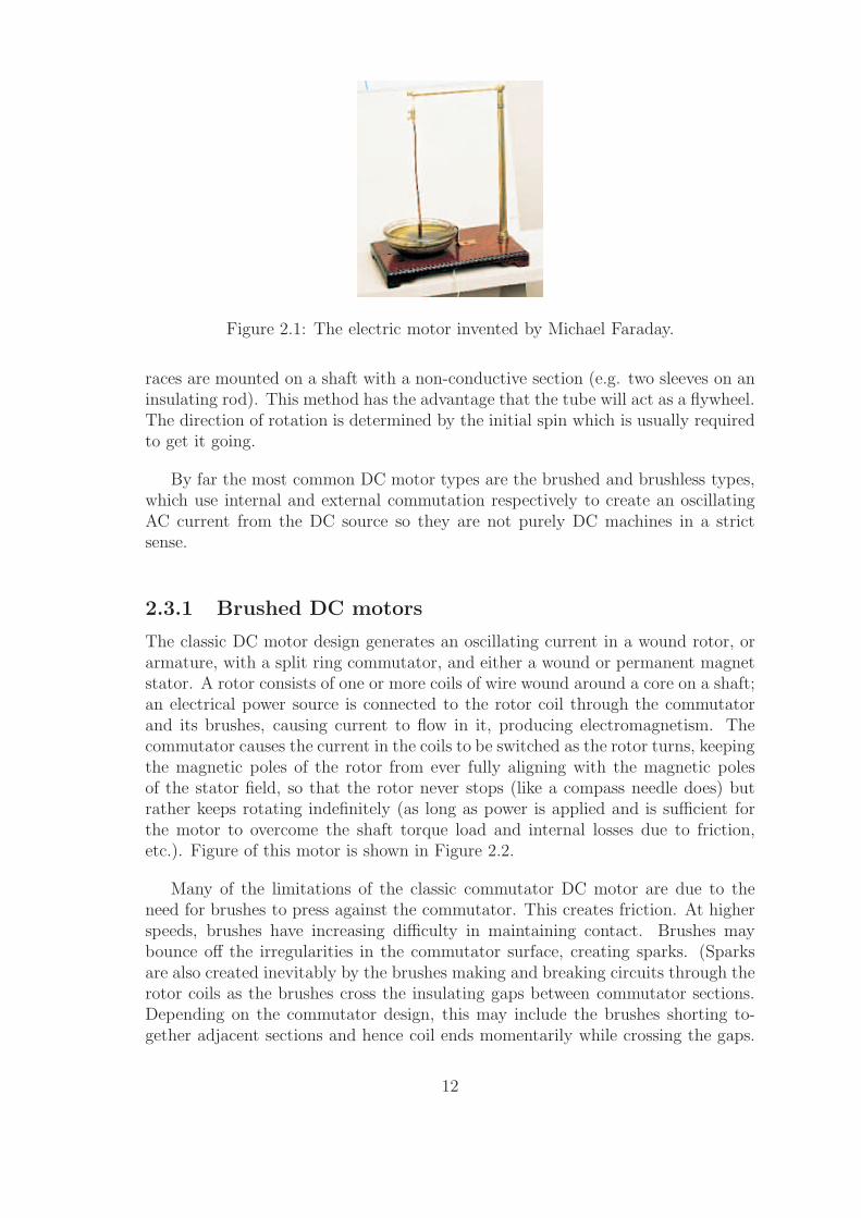
Figure 2.1: The electric motor invented by Michael Faraday.

races are mounted on a shaft with a non-conductive section (e.g. two sleeves on aninsulating rod). This method has the advantage that the tube will act as a flywheel.The direction of rotation is determined by the initial spin which is usually requiredto get it going.

By far the most common DC motor types are the brushed and brushless types,which use internal and external commutation respectively to create an oscillatingAC current from the DC source so they are not purely DC machines in a strictsense.

2.3.1 Brushed DC motors

The classic DC motor design generates an oscillating current in a wound rotor, orarmature, with a split ring commutator, and either a wound or permanent magnetstator. A rotor consists of one or more coils of wire wound around a core on a shaft;an electrical power source is connected to the rotor coil through the commutatorand its brushes, causing current to flow in it, producing electromagnetism. Thecommutator causes the current in the coils to be switched as the rotor turns, keepingthe magnetic poles of the rotor from ever fully aligning with the magnetic polesof the stator field, so that the rotor never stops (like a compass needle does) butrather keeps rotating indefinitely (as long as power is applied and is sufficient forthe motor to overcome the shaft torque load and internal losses due to friction,etc.). Figure of this motor is shown in Figure 2.2.

Many of the limitations of the classic commutator DC motor are due to theneed for brushes to press against the commutator. This creates friction. At higherspeeds, brushes have increasing difficulty in maintaining contact. Brushes maybounce off the irregularities in the commutator surface, creating sparks. (Sparksare also created inevitably by the brushes making and breaking circuits through therotor coils as the brushes cross the insulating gaps between commutator sections.Depending on the commutator design, this may include the brushes shorting to-gether adjacent sections and hence coil ends momentarily while crossing the gaps.

12

CommutatorShaft

Windings Armature

BrushShaft

Brush

Figure 2.2: Brushed DC motor.

Furthermore, the inductance of the rotor coils causes the voltage across each torise when its circuit is opened, increasing the sparking of the brushes.) This spark-ing limits the maximum speed of the machine, as too-rapid sparking will overheat,erode, or even melt the commutator. The current density per unit area of thebrushes, in combination with their resistivity, limits the output of the motor. Themaking and breaking of electric contact also causes electrical noise, and the sparksadditionally cause RFI. Brushes eventually wear out and require replacement, andthe commutator itself is subject to wear and maintenance (on larger motors) orreplacement (on small motors). The commutator assembly on a large machine is acostly element, requiring precision assembly of many parts. On small motors, thecommutator is usually permanently integrated into the rotor, so replacing it usuallyrequires replacing the whole rotor.

Large brushes are desired for a larger brush contact area to maximize motor out-put, but small brushes are desired for low mass to maximize the speed at which themotor can run without the brushes excessively bouncing and sparking (comparableto the problem of ”valve float” in internal combustion engines). (Small brushesare also desirable for lower cost.) Stiffer brush springs can also be used to makebrushes of a given mass work at a higher speed, but at the cost of greater frictionlosses (lower efficiency) and accelerated brush and commutator wear. Therefore,DC motor brush design entails a trade-off between output power, speed, and effi-ciency/wear. Types of DC motors are permanent magnet, separately, shunt, seriesand compound.

2.4 Principle of Operation

2.4.1 Production of Torque

Consider a wire carrying a current I suspended in a magnetic field of uniform fluxdensity B, as shown in Figure 2.3, where the direction of the current is at rightangles to the flux.

13

Figure 2.3: Production of torque.

Ampere’s law tells us that a force F will be produced whose direction is orthog-onal to both the current and flux and whose magnitude is given by :

F = Bli (2.1)

where :

l is the length of wire within the field.i is the current flowing in the wire.

In a DC motor the field B is usually produced by means of a strong permanentmagnet. The flux is ’guided’ by means of a steel magnetic circuit to two pole facesas shown in Figure 2.4. This part of motor is known as the stator.

Figure 2.4: Production of magnetic field by permanent magnet.

Instead of having a single current-carrying wire, it is shaped into a coil so thatthe first conductor lies under the North pole face and the return conductor liesunder the South pole face, as shown in Figure 2.5. The coil is supported in themiddle on a shaft which rotates in bearings at either end of the motor. This partof the motor is known as the rotor or armature.

The net effect of the two forces - one upward and one downward - is to exert aturning moment or torque of value

14

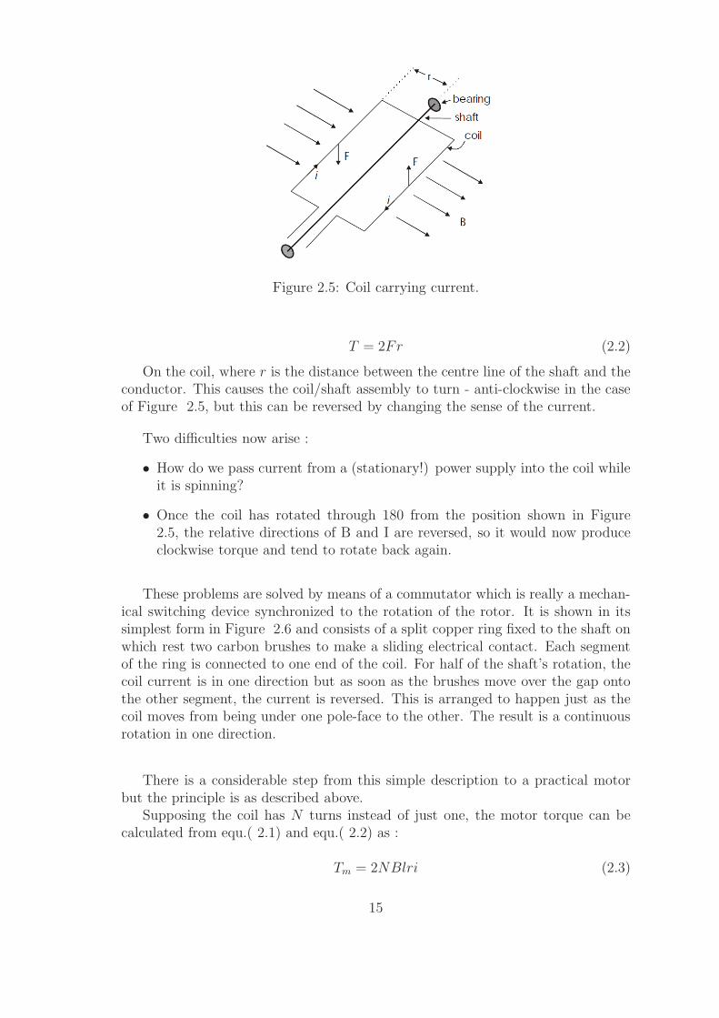
Figure 2.5: Coil carrying current.

T = 2Fr (2.2)

On the coil, where r is the distance between the centre line of the shaft and theconductor. This causes the coil/shaft assembly to turn - anti-clockwise in the caseof Figure 2.5, but this can be reversed by changing the sense of the current.

Two difficulties now arise :

• How do we pass current from a (stationary!) power supply into the coil whileit is spinning?

• Once the coil has rotated through 180 from the position shown in Figure2.5, the relative directions of B and I are reversed, so it would now produceclockwise torque and tend to rotate back again.

These problems are solved by means of a commutator which is really a mechan-ical switching device synchronized to the rotation of the rotor. It is shown in itssimplest form in Figure 2.6 and consists of a split copper ring fixed to the shaft onwhich rest two carbon brushes to make a sliding electrical contact. Each segmentof the ring is connected to one end of the coil. For half of the shaft’s rotation, thecoil current is in one direction but as soon as the brushes move over the gap ontothe other segment, the current is reversed. This is arranged to happen just as thecoil moves from being under one pole-face to the other. The result is a continuousrotation in one direction.

There is a considerable step from this simple description to a practical motorbut the principle is as described above.

Supposing the coil has N turns instead of just one, the motor torque can becalculated from equ.( 2.1) and equ.( 2.2) as :

Tm = 2NBlri (2.3)

15

Figure 2.6: Split copper ring.

Note here that N , B, l, and r are constant for any particular motor so we cansay :

Tm = Kti (2.4)

where Kt is known as the motor’s torque constant, with units NmA−1.Equation 2.5 is the first of the equations which form the d.c. motor model.

2.4.2 Generated E.M.F.

According to Faraday’s law, a coil of length l rotating in an uniform magnetic fieldof flux density B will generate an E.M.F. given by :

e = −dλ

dt(2.5)

where λ is the flux linking the coil.Consider the coil of length l and radius r to be at an angle θm to the magnetic

field between the pole-faces, as shown in cross-section in Figure 2.7.

Figure 2.7: Cross section of dc motor

The magnetic flux linking the coil is given by:

φ = Bl2r cos θm (2.6)

16

and the magnetic flux linkage is:

λ = Nφ = 2NBlr cos θm (2.7)

If the coil is rotating at a constant angular speed ωm then its angle at any timet is ωmt. From equ.( 2.5) we then have:

e = −dλ

dt= −2NBlr

d(cosωmt)

dte = −2NBlr(−ωm sin (ωmt) = 2NBlrωm sin (ωmt)

(2.8)When the coil is at θm = 90, the term sin (ωmt) = 1 and:

e = 2NBlrωm = Ktωm (2.9)

Note that the same constant Kt appears in equ.( 2.9) as in equ.( 2.3) althoughit is conventional here to call it the back emf constant, with units of (volts perradian per second).

Equation ( 2.9) is the second of the equations which form the dc motor model.

2.4.3 Motor Modeling and Simulation

A common actuator in control systems is the DC motor [20, 21]. It directly pro-vides rotary motion and, coupled with wheels or drums and cables, can providetransitional motion. The electric circuit of the armature and the free body diagramof the rotor are shown in the following Figure 2.8.

Tf

B

J

T=K it a

+

-

if

Vf

+

-

ia

V

++ -- RaLa

+

-

E=Ke

Figure 2.8: Complete equivalent model for dc motor

The motor torque, T, is related to the armature current, ia, by a constant factorKt. The back emf, E, is related to the rotational velocity by the constant factor Ke

as in the following equations:

T = Ktia (2.10)

17

E = Keω (2.11)

The dynamic of the dc motor may be expressed by the following equations:

V = Raia + Ladiadt

+Keω (2.12)

Ktia = Jdω

dt+Bω + Tf (2.13)

In the state-space form, the equations above can be expressed by choosing therotational speed and electric current as the state variables and the voltage as aninput. The output is chosen to be the rotational speed or current, so by representingequ.( 2.12) and equ.( 2.13) in a model of state space form provides:

[

iaω

]

=

[

−Ra

La

−Ke

La

Kt

J−B

J

] [

iaω

]

+

[

1La

0

0 − 1J

] [

VTf

]

(2.14)

Using Laplace Transforms, the above modeling equations can be expressed interms of s.

Armature current can be expressed using laplace transform as following:

Ia(s) =

[

1

Las+Ra

]

[V (s)−Keω(s)] (2.15)

Rotational speed also expressed as following:

Ia(s) =

[

1

sJ +B

]

[KtIa(s)− Tf ] (2.16)

Now the block diagram of dc motor can be derived from the above equations asshown in Figure (2.9).

V +-

+-

Ke

Kt

Tf

1s

11Ia Tg

Js+BLas+Ra

Figure 2.9: The Block diagram of dc motor

The transfer function from the input armature voltage, V (s), to the outputarmature current, Ia(s), directly follows:

Ia(s)

V (s)=

1La

(s+ BJ)

s2 + s(Ra

La

+ BJ) + (RaB

LaJ+ KeKt

LaJ)

(2.17)

18

The transfer function in equ.( 4.2) may be expressed as following:

Ia(s)

V (s)=

s+ BJ

Las2 + s(Ra +LaBJ

) + (RaBJ

+ KeKt

J)

(2.18)

The transfer function from the input armature voltage, V (s), to the rotationalspeed in (rad/sec), W (s), directly follows:

W (s)

V (s)=

Kt

LaJ

s2 + s(Ra

La

+ BJ) + (RaB

LaJ+ KeKt

LaJ)

(2.19)

or by the following equation:

W (s)

V (s)=

Kt

J

Las2 + s(Ra +LaBJ

) + (RaBJ

+ KeKt

J)

(2.20)

In metric (SI) units Kt (N.mA

) is equal to Ke ( V oltsrad/sec

) as justified in the litera-

ture [22].

2.5 Parameters Identification

Once we installed the experimental system and acquired the required signals needed,the stage of parameters identification of dc motor is now ready. The parametersneeded for identification is summarized in table 2.1:

There are various possible approaches used for parameters identification, theseapproaches are studied in details and trying to apply them on the experimentalsystem, these approaches are:

• Pseudo inverse technique

• Nonlinear least-square method

• Pattern search algorithm

2.5.1 Pseudo Inverse Technique

The pseudo inverse technique is a method capable of identifying an equivalent dis-crete transfer function of simple systems like motor, thermal system, mass dampersystems etc with no zeros (only poles).

The transfer function of the system (speed over armature voltage) in z domainis of the following form:

W (z)

V (z)=

b0z2

z2 + a1z + a2(2.21)

19

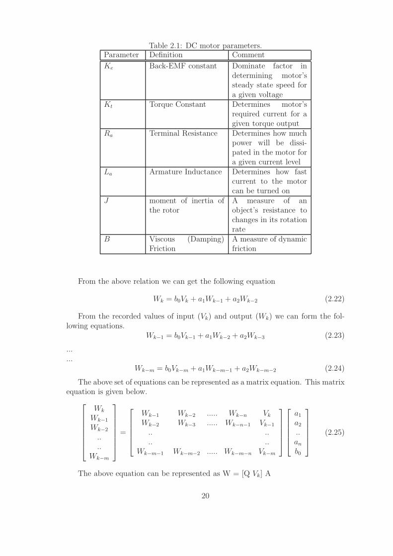
Table 2.1: DC motor parameters.Parameter Definition Comment

Ke Back-EMF constant Dominate factor indetermining motor’ssteady state speed fora given voltage

Kt Torque Constant Determines motor’srequired current for agiven torque output

Ra Terminal Resistance Determines how muchpower will be dissi-pated in the motor fora given current level

La Armature Inductance Determines how fastcurrent to the motorcan be turned on

J moment of inertia ofthe rotor

A measure of anobject’s resistance tochanges in its rotationrate

B Viscous (Damping)Friction

A measure of dynamicfriction

From the above relation we can get the following equation

Wk = b0Vk + a1Wk−1 + a2Wk−2 (2.22)

From the recorded values of input (Vk) and output (Wk) we can form the fol-lowing equations.

Wk−1 = b0Vk−1 + a1Wk−2 + a2Wk−3 (2.23)

...

...Wk−m = b0Vk−m + a1Wk−m−1 + a2Wk−m−2 (2.24)

The above set of equations can be represented as a matrix equation. This matrixequation is given below.

Wk

Wk−1

Wk−2

..

..Wk−m

=

Wk−1 Wk−2 ..... Wk−n Vk

Wk−2 Wk−3 ..... Wk−n−1 Vk−1

.. ..

.. ..Wk−m−1 Wk−m−2 ..... Wk−m−n Vk−m

a1a2..anb0

(2.25)

The above equation can be represented as W = [Q Vk] A

20

Let X = [Q Vk]Q : Matrix built using Wk values as shown in the above matrix equation.X : Matrix built using [Q V]W = X ASize of the matrices in the above matrix equation is given below.W : (m+1) x 1X : (m+1) x (n+1)A : (n+1) x 1Premultiply Matrix equation M1 by XT on both sidesXTW = XTXAPremultiply by [XTX ]−1 on both sides of the Matrix Eqn[XTX ]−1.XT .W = [XTX ]−1[XTX ]A[XTX ]−1.XT .W = AA = [[XTX ]−1.XT ]WWhere [[XTX ]−1.XT ] is called as the pseudo inverse of X

OutputPhysicalsystem

PC with DataAcquisition

system

Input

Figure 2.10: Experimental setup requirement

Figure ( 2.10) shows the experimental setup requirement prior to the parameteridentification. This is the recording phase.

1. Deploy a data acquisition system, which can record the input and output atthe required sampling frequency (according to the system dynamics).

2. Feed the system with rich inputs. (Inputs must change with time).

3. Record the inputs and corresponding outputs simultaneously using this dataacquisition system

Now we have all the information required for identifying the mathematical modelof the system. This method is programmed in MATLAB and is applied to our dcmotor signals and give us these the transfer function of DC motor in Z-domain butit’s difficult to extract the parameters from this transfer function. So we will lookat another technique which may help us to find these parameters.

21

2.5.2 Nonlinear Least-Square Method

Nonlinear least squares regression extends linear least squares regression for usewith a much larger and more general class of functions. Almost any function thatcan be written in closed form can be incorporated in a nonlinear regression model.Unlike linear regression, there are very few limitations on the way parameters canbe used in the functional part of a nonlinear regression model. The way in whichthe unknown parameters in the function are estimated, however, is conceptuallythe same as it is in linear least squares regression.

As the name suggests, a nonlinear model is any model of the basic form:

y = f(x; β) + ǫ (2.26)

in which:

1. the functional part of the model is not linear with respect to the unknownparameters, β0, β1, ...

2. the method of least squares is used to estimate the values of the unknownparameters.

Due to the way in which the unknown parameters of the function are usuallyestimated, however, it is often much easier to work with models that meettwo additional criteria:

3. the function is smooth with respect to the unknown parameters.

4. the least squares criterion that is used to obtain the parameter estimates hasa unique solution.

These last two criteria are not essential parts of the definition of a nonlinearleast squares model, but are of practical importance.

The biggest advantage of nonlinear least squares regression over many othertechniques is the broad range of functions that can be fit. Although many scientificand engineering processes can be described well using linear models, or other rel-atively simple types of models, there are many other processes that are inherentlynonlinear. For example, the strengthening of concrete as it cures is a nonlinearprocess. Research on concrete strength shows that the strength increases quicklyat first and then levels off, or approaches an asymptote in mathematical terms, overtime. Linear models do not describe processes that asymptote very well because forall linear functions the function value can’t increase or decrease at a declining rateas the explanatory variables go to the extremes. There are many types of nonlinearmodels, on the other hand, that describe the asymptotic behavior of a process well.Like the asymptotic behavior of some processes, other features of physical processescan often be expressed more easily using nonlinear models than with simpler modeltypes.

Being a ”least squares” procedure, nonlinear least squares has some of the sameadvantages (and disadvantages) that linear least squares regression has over other

22

methods. One common advantage is efficient use of data. Nonlinear regressioncan produce good estimates of the unknown parameters in the model with rela-tively small data sets. Another advantage that nonlinear least squares shares withlinear least squares is a fairly well-developed theory for computing confidence, pre-diction and calibration intervals to answer scientific and engineering questions. Inmost cases the probabilistic interpretation of the intervals produced by nonlinearregression are only approximately correct, but these intervals still work very wellin practice.

The major cost of moving to nonlinear least squares regression from simplermodeling techniques like linear least squares is the need to use iterative optimizationprocedures to compute the parameter estimates. With functions that are linearin the parameters, the least squares estimates of the parameters can always beobtained analytically, while that is generally not the case with nonlinear models.The use of iterative procedures requires the user to provide starting values for theunknown parameters before the software can begin the optimization. The startingvalues must be reasonably close to the as yet unknown parameter estimates or theoptimization procedure may not converge. Bad starting values can also cause thesoftware to converge to a local minimum rather than the global minimum thatdefines the least squares estimates.

Disadvantages shared with the linear least squares procedure includes a strongsensitivity to outliers. Just as in a linear least squares analysis, the presence of oneor two outliers in the data can seriously affect the results of a nonlinear analysis.In addition there are unfortunately fewer model validation tools for the detectionof outliers in nonlinear regression than there are for linear regression

2.5.3 Pattern Search Algorithm

Pattern search is an attractive alternative to the genetic algorithm, as it is oftencomputationally less expensive and can minimize the same types of functions. Ad-ditionally, the Genetic Algorithm and Direct Search Toolbox includes a patternsearch method that can solve problems with linear constraints [23].

Pattern search operates by searching a set of points called a pattern, whichexpands or shrinks depending on whether any point within the pattern has a lowerobjective function value than the current point. The search stops after a minimumpattern size is reached. Like the genetic algorithm, the pattern search algorithmdoes not use derivatives to determine descent, and so it works well on nondiffer-entiable, stochastic, and discontinuous objective functions. Pattern search is alsoeffective at finding a global minimum because of the nature of its search.

A pattern is a set of vectors vi that the pattern search algorithm uses to deter-mine which points to search at each iteration. The set vi is defined by the number ofindependent variables in the objective function, N, and the positive basis set. Twocommonly used positive basis sets in pattern search algorithms are the maximalbasis, with 2N vectors, and the minimal basis, with N+1 vectors.

23

With Generalized Pattern Search Algorithm (GPS) , the collection of vectorsthat form the pattern are fixed-direction vectors. For example, if there are threeindependent variables in the optimization problem, the default for a 2N positivebasis consists of the following pattern vectors:

v1=[1 0 0], v2=[0 1 0], v3=[0 0 1]v4=[-1 0 0], v5=[0 -1 0], v6=[0 0 -1]

An N+1 positive basis consists of the following default pattern vectors.

v1=[1 0 0], v2=[0 1 0], v3=[0 0 1]v4=[-1 -1 -1]

with Mesh Adaptive Search Algorithm (MADS), the collection of vectors thatform the pattern are randomly selected by the algorithm. Depending on the pollmethod choice, the number of vectors selected will be 2N or N+1. As in GPS, 2Nvectors consist of N vectors and their N negatives, while N+1 vectors consist of Nvectors and one that is the negative of the sum of the others.

At each step, the pattern search algorithm searches a set of points, called a mesh,for a point that improves the objective function. The GPS and MADS algorithmsform the mesh by

• Generating a set of vectors di by multiplying each pattern vector vi by a scalarm. m is called the mesh size.

• Adding the di to the current pointthe point with the best objective functionvalue found at the previous step.

The pattern vector that produces a mesh point is called its direction.

At each step, the algorithm polls the points in the current mesh by computingtheir objective function values. When the Complete poll option has the (default)setting Off, the algorithm stops polling the mesh points as soon as it finds a pointwhose objective function value is less than that of the current point. If this occurs,the poll is called successful and the point it finds becomes the current point at thenext iteration.

The algorithm only computes the mesh points and their objective function valuesup to the point at which it stops the poll. If the algorithm fails to find a pointthat improves the objective function, the poll is called unsuccessful and the currentpoint stays the same at the next iteration.

When the Complete poll option has the setting On, the algorithm computesthe objective function values at all mesh points. The algorithm then compares themesh point with the smallest objective function value to the current point. If thatmesh point has a smaller value than the current point, the poll is successful.

24

After polling, the algorithm changes the value of the mesh size m. The defaultis to multiply m by 2 after a successful poll, and by 0.5 after an unsuccessful poll.

The pattern search algorithms find a sequence of points, x0, x1, x2, ... , thatapproaches an optimal point. The value of the objective function either decreasesor remains the same from each point in the sequence to the next

The algorithm stops when any of the following conditions occurs:

• The mesh size is less than Mesh tolerance.

• The number of iterations performed by the algorithm reaches the value ofMax iteration.

• The total number of objective function evaluations performed by the algo-rithm reaches the value of Max function evaluations.

• The time, in seconds, the algorithm runs until it reaches the value of Timelimit.

• The distance between the point found in two consecutive iterations and themesh size are both less than X tolerance.

• The change in the objective function in two consecutive iterations and themesh size are both less than Function tolerance.

Nonlinear constraint tolerance is not used as stopping criterion. It determinesthe feasibility with respect to nonlinear constraints.

25

Chapter 3

System Hardware Development

3.1 Introduction

System Hardware development begin with searching for DC motor that may becontain on parameters information, unfortunately we can’t find this kind of motor.Finally, we find a DC motor to perform our experiments. The DC motor is thebackbone of our system. This motor has the nominal characteristics printed on itsnameplate as shown in Table ( 3.1).

Table 3.1: Specification of experimental dc motor.Rated power 200 WRated speed 1500 rpmArmature rated voltage 110 VArmature rated current 3 AField voltage 2.5 VField current 1.3 AMagnetic break 24 V

This DC motor is shown in Figure 3.1.The DC motor have the following wires:

• Two wires for the armature terminals.

• Two wires for the field terminals.

• Two wires for the magnetic break (24VDC).

• Two wires for overheat protection.

From the figure drawn on its nameplate it’s clearly that it’s series wound motor,but its characteristics is different than permanent magnet dc motor characteristicsthat will studied in out thesis, so we try to change to use it as a permanent magnetDC motor by applying a constant voltage to its field terminals. This is done by

26

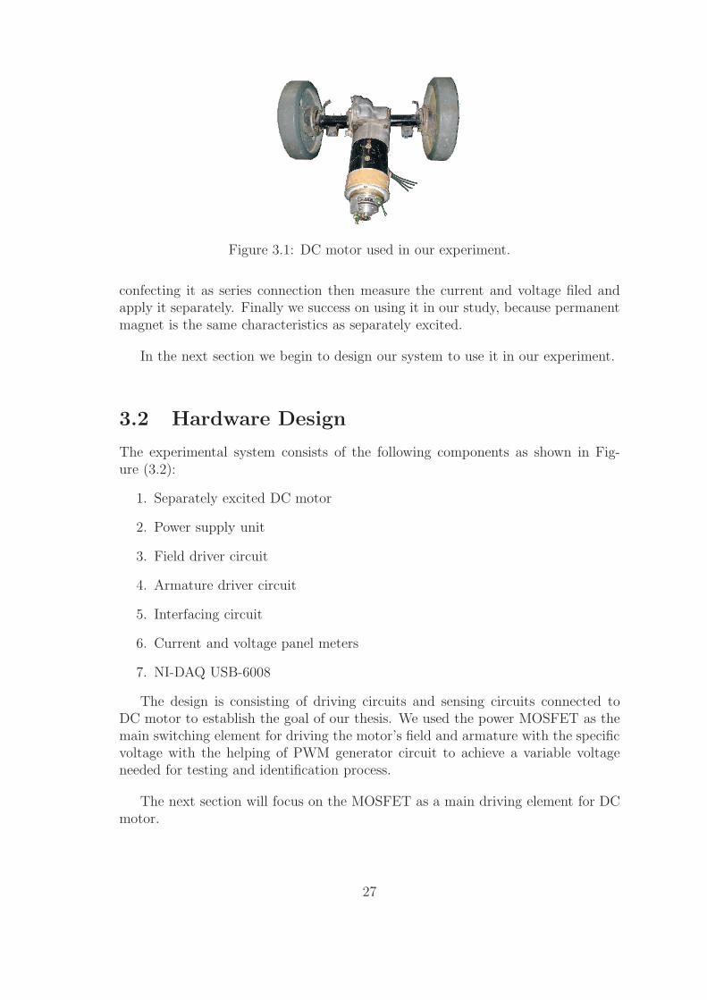
Figure 3.1: DC motor used in our experiment.

confecting it as series connection then measure the current and voltage filed andapply it separately. Finally we success on using it in our study, because permanentmagnet is the same characteristics as separately excited.

In the next section we begin to design our system to use it in our experiment.

3.2 Hardware Design

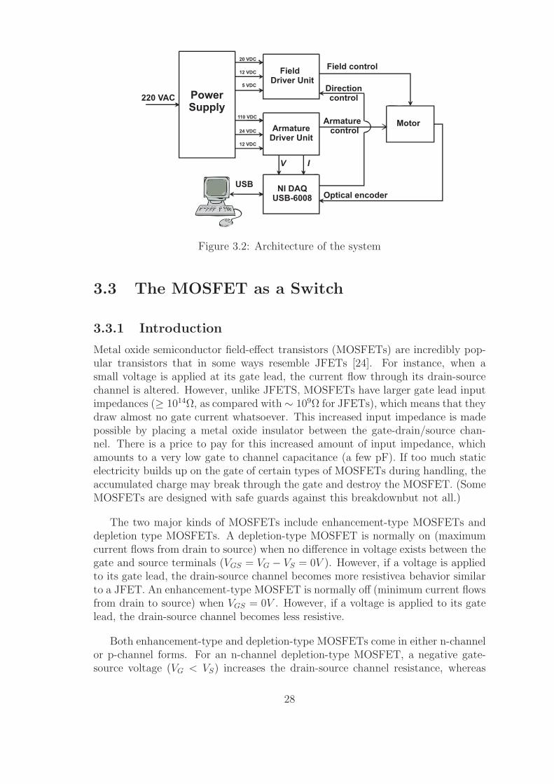
The experimental system consists of the following components as shown in Fig-ure (3.2):

1. Separately excited DC motor

2. Power supply unit

3. Field driver circuit

4. Armature driver circuit

5. Interfacing circuit

6. Current and voltage panel meters

7. NI-DAQ USB-6008

The design is consisting of driving circuits and sensing circuits connected toDC motor to establish the goal of our thesis. We used the power MOSFET as themain switching element for driving the motor’s field and armature with the specificvoltage with the helping of PWM generator circuit to achieve a variable voltageneeded for testing and identification process.

The next section will focus on the MOSFET as a main driving element for DCmotor.

27

Motor

Field control

Armaturecontrol

Optical encoderNI DAQ

USB-6008

ArmatureDriver Unit

FieldDriver Unit

USB

PowerSupply

220 VAC

20 VDC

12 VDC

5 VDC

110 VDC

24 VDC

12 VDC

V I

Directioncontrol

Figure 3.2: Architecture of the system

3.3 The MOSFET as a Switch

3.3.1 Introduction

Metal oxide semiconductor field-effect transistors (MOSFETs) are incredibly pop-ular transistors that in some ways resemble JFETs [24]. For instance, when asmall voltage is applied at its gate lead, the current flow through its drain-sourcechannel is altered. However, unlike JFETS, MOSFETs have larger gate lead inputimpedances (≥ 1014Ω, as compared with∼ 109Ω for JFETs), which means that theydraw almost no gate current whatsoever. This increased input impedance is madepossible by placing a metal oxide insulator between the gate-drain/source chan-nel. There is a price to pay for this increased amount of input impedance, whichamounts to a very low gate to channel capacitance (a few pF). If too much staticelectricity builds up on the gate of certain types of MOSFETs during handling, theaccumulated charge may break through the gate and destroy the MOSFET. (SomeMOSFETs are designed with safe guards against this breakdownbut not all.)

The two major kinds of MOSFETs include enhancement-type MOSFETs anddepletion type MOSFETs. A depletion-type MOSFET is normally on (maximumcurrent flows from drain to source) when no difference in voltage exists between thegate and source terminals (VGS = VG − VS = 0V ). However, if a voltage is appliedto its gate lead, the drain-source channel becomes more resistivea behavior similarto a JFET. An enhancement-type MOSFET is normally off (minimum current flowsfrom drain to source) when VGS = 0V . However, if a voltage is applied to its gatelead, the drain-source channel becomes less resistive.

Both enhancement-type and depletion-type MOSFETs come in either n-channelor p-channel forms. For an n-channel depletion-type MOSFET, a negative gate-source voltage (VG < VS) increases the drain-source channel resistance, whereas

28

for a p-channel depletion-type MOSFET, a positive gate-source voltage (VG > VS)increases the channel resistance. For an n-channel enhancement-type MOSFET,a positive gate-source voltage (VG > VS) decreases the drain-source channel resis-tance, whereas for a p-channel enhancement-type MOSFET, a negative gate-sourcevoltage (VG < VS) decreases the channel resistance.

MOSFETs are perhaps the most popular transistors used today; they draw verylittle input current, are easy to make (require few ingredients), can be made ex-tremely small, and consume very little power. In terms of applications, MOSFETsare used in ultrahigh input impedance amplifier circuits, voltage-controlled resistorcircuits, switching circuits, and found with large-scale integrated digital ICs.

Like JFETs, MOSFETs have small transconductance values when comparedwith bipolar transistors. In terms of amplifier applications, this can lead to de-creased gain values. For this reason, you will rarely see MOSFETs in simple am-plifier circuits, unless there is a need for ultrahigh input impedance and low inputcurrent features.

As the motor load is inductive, a simple ”Free-wheeling” diode is connectedacross the load to dissipate any back emf generated by the motor when the MOS-FET turns it ”OFF”. The Zener diode is used to prevent excessive gate-sourceinput voltages.

3.3.2 Choosing a MOSFET

Choosing the right power MOSFET that will be used to drive the sufficient currentto DC motor is an important part. This choice depends on load specifications, themaximum voltage and maximum current of the load, because MOSFETs are gen-erally advertised by their maximum drain current, maximum drain-source voltageand static drain-source on resistance. To examine the parameters of MOSFETs, itis useful to have a sample datasheet to hand. If you cannot find a single MOSFETwith a high enough maximum drain current, then you can connect more than onein parallel.

Selecting the right MOSFET driver for the application requires a thoroughunderstanding of power dissipation in relation to the MOSFET’s gate charge andoperating frequencies. For example, charging and discharging a MOSFET’s gaterequires the same amount of energy, regardless of how fast or slow the gate voltagetransitions are [25].

A MOSFET driver’s power dissipation capabilities are determined by three keyelements:

• Power dissipation due to charging and discharging the MOSFET’s gate ca-pacitance.

• Power dissipation due to the MOSFET driver’s quiescent-current draw.

29

• Power dissipation due to cross-conduction (shoot-through) current in theMOSFET driver.

Of these three elements, power dissipation due to the charging and dischargingof the MOSFET’s gate capacitance is most important, especially at lower switchingfrequencies. This is given by:

Pc = Cg × V 2dd × F (3.1)

where Cg = MOSFET gate capacitance, Vdd = supply voltage of MOSFETdriver (V), and F = switching frequency.

In addition to power dissipation, designers must understand the peak drivecurrent required from the MOSFET driver and the associated turn-on and -offtimes. Matching the MOSFET driver to the MOSFET in an application dependson how fast the application requires the power MOSFET to be switched on and off.

The optimum rise or fall time in any application is based on many requirements,such as EMI, switching losses, lead/circuit inductance, and switching frequency.The relationship between gate capacitance, transition times, and the MOSFETdriver current rating is given by:

dT = [dV × C]/I (3.2)

where dT= turn-on/turn-off time, dV = gate voltage, C = gate capacitance,and I = MOSFET peak drive current.

The total MOSFET gate capacitance can be properly determined by looking atthe total gate charge (QG). Gate charge QG is given by:

QG = C × V (3.3)

Then I = QG/dT .

This method assumes a constant current. A good rule of thumb is that theaverage value found is half of the MOSFET driver’s peak current rating. MOSFETdrivers are rated by the driver output peak current drive capability.

The peak current rating is typically stated for the part’s maximum bias voltage.This means that, if the MOSFET driver is being used with a lower bias voltage, itspeak current drive capability will be reduced.

Another method designers can use to selecting the appropriate MOSFET driveris to use a time-constant approach. In this approach, the MOSFET driver resis-tance, any external gate resistance, and the lumped capacitance are used.

Tcharge = ((Rdriver +Rgate)× Ctotal)× TC (3.4)

where Rdriver = RDS(on) of the output driver stage, Rgate = any external gateresistance between the driver and MOSFET gate, Ctotal = total gate capacitance,and TC = number of time constants.

30

3.3.3 MOSFET Gate Driver

To turn a power MOSFET on, the gate terminal must be set to a voltage at least10 volts greater than the source terminal (about 4 volts for logic level MOSFETs).This is comfortably above the V gsth parameter.

One feature of power MOSFETs is that they have a large stray capacitancebetween the gate and the other terminals, Ciss. The effect of this is that when thepulse to the gate terminal arrives, it must first charge this capacitance up beforethe gate voltage can reach the 10 volts required. The gate terminal then effectivelydoes take current. Therefore the circuit that drives the gate terminal should becapable of supplying a reasonable current so the stray capacitance can be chargedup as quickly as possible. The best way to do this is to use a dedicated MOSFETdriver chip.

There are a lot of MOSFET driver chips available from several companies. Someare shown with links to the datasheets in the table below. Some require the MOS-FET source terminal to be grounded (for the lower 2 MOSFETs in a full bridgeor just a simple switching circuit). Some can drive a MOSFET with the sourceat a higher voltage. These have an on-chip charge pump, which means they cangenerate the 22 volts required to turn the upper MOSFET in a full bridge on. TheTDA340 even controls the swicthing sequence for you. Some can supply as muchas 6 Amps current as a very short pulse to charge up the stray gate capacitance.

Often you will see a low value resistor between the MOSFET driver and theMOSFET gate terminal. This is to dampen down any ringing oscillations caused bythe lead inductance and gate capacitance which can otherwise exceed the maximumvoltage allowed on the gate terminal. It also slows down the rate at which theMOSFET turns on and off. This can be useful if the intrinsic diodes in the MOSFETdo not turn on fast enough.

Table 3.2: MOSFET Drivers.Manufacturer IC Features

Maxim and others ICL 7667 Dual inverting driverMaxim MAX622/MAX1614 High side driversMaxim MAX626/MAX627/MAX628 Low side driversInternational Recti-fier

IR2110 High and low sidedriver

Harris / Intersil HIP4080/4081/4082 Full bridge driversSGS Thomson (ST) TD340 New full bridge

driver with analogueor PWM speeddemand input

31

3.4 Pulse Width Modulation (PWM)

PWM, or Pulse Width Modulation is a powerful way of controlling analog circuitsand systems, using the digital outputs of microprocessors. Defining the term, wecan say that PWM is the way we control a digital signal simulating an analog one,by means of altering it’s state and frequency of this.

The PWM is actually a square wave modulated. This modulation infects on thefrequency (clock cycle) and the duty cycle of the signal. PWM signal is character-ized from the duty clock and the duty cycle. The amplitude of the signal remainsstable during time (except of course from the rising and falling ramps). The clockcycle is measured in Hz and the duty cycle is measured in hundred percent (Theseare the basic parameters that characterizes a PWM signal.

One of the most popular usages of PWM is the control of voltage deliveredto loads. Those loads could be for example an LED which would utilize a LEDdimmer, or a motor that could be a simple DC motor and would be converted intoa controlled speed DC motor, as used for example in the modern PC motherboardfans. A PWM signal with 100% duty cycle would deliver 100% of the voltage. Itwould be like a DC power supply. But by altering the duty cycle, the result is toreduce the area of the power delivered to the load. The total power delivered tothe connected load each time, is the area under the positive state of the PWM. Itis clearly seen that by altering the duty cycle, we can alter the power delivered bythe supply. And because the wave form is a square wave, the power supplied eachtime is calculated by equ.( 3.5).

PDelivered = PSupplied ×DutyCycle (3.5)

Due to the efficiency and simplicity of PWM, as well as the flexibility of thismodulation type, there are numbers of applications that it can take place. Us-ing PWM someone can modulate transmit and/or storage analog signals like au-dio/voice telecommunications and music. Switching power supplies that uses thistechnology are much more energy efficient than the classic power supplies, reachingup to 60% power saving! The output power and/or voltage can be controlled eitherdigitally using a micro-controller or with the old classic potentiometer. Steppermotors can be easily controlled using PWM, as well as DC motors. The torque andspeed of a DC motor can be controlled by altering the voltage or the duty cycleof the PWM easily. PWM is widely used in dimmer circuits that could control avariety of lamps including LEDs.

In our thesis a Pulse width modulation (PWM) signal at a frequency of 250 Hzis used to adjust the magnitude of excitation voltage applied on the field terminals.Usually the frequency is set to be at least 5 times higher than the rotation speed ofthe motor. In our case the max speed of motor is 1500 rpm (25 rps) the frequency isbetter be higher than 5× 25Hz = 125Hz. A frequency of 250 Hz will be a suitablevalue. Reversing the rotation direction of the motor is easily done by reversing thefield excitation. Therefore an additional relay is employed to facilitate user control

32

Figure 3.3: A Practical PWM Circuit.

of motor direction. Field driver circuit is shown in Figure ( 3.4), Figure (B.1) andFigure (B.2).

Figure 3.4: Field driver circuit.

Armature driver circuit is the same version of filed driver circuit. Voltage andcurrent sensing components are added in this circuit. Moreover, a 100nf capacitor isconnected across the motor armature in order to reduce electromagnetic interference(EMI). Both field and armature driver circuits are featured by the ability to becontrolled locally or remotely via the data acquisition card. Two digital panelmeters are used to monitor the current and voltage of the armature winding anda third one is used to monitor field current. Armature driver circuit is shown inFigure ( 3.5), Figure (B.3) and Figure (B.4).

33

Figure 3.5: Armature driver circuit.

3.5 Power Supply

The power supply unit consists of a traditional components which supply all neces-sary voltage levels. Separate voltage levels are required for the field driver unit andfor the armature driver unit. The first unit requires voltage supplies of +20VDC,+12VDC and +5VDC. On the other hand, the second unit requires +110VDC,+24VDC and +12VDC voltage levels. Figure 3.6 show the final design of thepower supply box. The schematics for the power circuits are in Figure (B.5) andFigure (B.6).

Figure 3.6: Power Box.

Important thing in power supply is to use an isolated transformers, because ifthe transformer is not isolated so it’s easy for interference to cause problems anddamage to electronic components.

34

3.6 Voltage Doubler

A voltage doubler is an electric circuit with an AC input and a DC output of roughlytwice the peak input voltage. They are a variety of voltage multiplier circuit andare often, but not always, a single stage of a general form of such circuits. Theterm is usually applied to circuits consisting of rectifying diodes and capacitorsonly, other means of doubling voltages are not included [31].

The main goal for using this circuit is to double the power source of 12V toget +24VDC suitable to drive the magnetic break of dc motor. The schematic ofthe circuit used is shown in Figure ( 3.7). The circuits used two diodes and twocapacitors beside the transformer and with a +24VDC regulator.

Figure 3.7: Voltage Doubler circuit.

3.7 Sensors and Feedback Elements

3.7.1 Introduction

Sensors are a critical component in a motor control system [26]. They are usedto sense the current, position, speed and direction of the rotating motor. Recentadvancements in sensor technology have improved the accuracy and reliability ofsensors, while reducing the cost. Many sensors are now available that integratethe sensor and signal-conditioning circuitry into a single package. In most motorcontrol systems, several sensors are used to provide feedback information on themotor. These sensors are used in the control loop and to improve the reliability bydetecting fault conditions that may damage the motor. As an example, Figure( 3.8)provides a block diagram of a DC motor control system to show the sensor feedbackprovided for a typical motor control.

A list of the sensors that can be used to feedback information to a DAQ ormicrocontroller are listed below:

• Current sensors

35

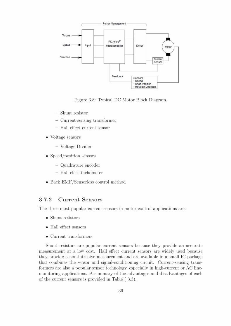
Figure 3.8: Typical DC Motor Block Diagram.

– Shunt resistor

– Current-sensing transformer

– Hall effect current sensor

• Voltage sensors

– Voltage Divider

• Speed/position sensors

– Quadrature encoder

– Hall efect tachometer

• Back EMF/Sensorless control method

3.7.2 Current Sensors

The three most popular current sensors in motor control applications are:

• Shunt resistors

• Hall effect sensors

• Current transformers

Shunt resistors are popular current sensors because they provide an accuratemeasurement at a low cost. Hall effect current sensors are widely used becausethey provide a non-intrusive measurement and are available in a small IC packagethat combines the sensor and signal-conditioning circuit. Current-sensing trans-formers are also a popular sensor technology, especially in high-current or AC line-monitoring applications. A summary of the advantages and disadvantages of eachof the current sensors is provided in Table ( 3.3).

36

Table 3.3: Current sensing methods.

Current Sensing Method Shunt Resistor Hall Effect Current SensingTransformer

Accuracy Good Good MediumAccuracyvs.Temperature

Good Poor Good

Cost Low High MediumIsolation No Yes YesHigh Current-MeasuringCapability

Poor Good Good

DC Offset Problem Yes No NoSaturation or HysteresisProblem

No Yes Yes

Power Consumption High Low LowIntrusive Measurement Yes No NoAC/DC Measurements Both Both Only AC

3.7.3 Shunt Resistors as a Current Sensor

Shunt resistors are a popular current-sensing sensor because of their low cost andgood accuracy. The voltage drop across a known low value resistor is monitoredin order to determine the current flowing through the load. If the resistor is smallin magnitude, the ‘voltage drop will be small and the measurement will not havea major effect on the motor circuit. The power dissipation of the resistance makescurrent shunts impractical for measurements of more than approximately 20 am-peres. The selection criteria of a shunt current resistor requires the evaluation ofseveral trade-offs, including:

• Increasing RSENSE increases the VSENSE voltage, which makes the voltageoffset (VOS) and input bias current offset (IOS) amplifier errors less signifi-cant.

• A large RSENSE value causes a voltage loss and a reduction in the powerefficiency due to the I2 × R loss of the resistor.

• A large RSENSE value will cause a voltage offset to the load in a low-sidemeasurement that may impact the EMI characteristics and noise sensitivityof the system.

• Special-purpose, low inductance resistors are required if the current has ahigh-frequency content.

• The power rating of RSENSE must be evaluated because the I2 × R powerdissipation can produce self heating and a change in the nominal resistanceof the shunt.

37

Special-purpose, shunt current measurement resistors are available from a num-ber of vendors. If standard resistors are used, it is recommended that metal-filmresistors be used rather than wire-wound resistors that have a relatively large in-ductance.

3.7.4 Speed/Position Sensor

A quadrature encoder can be used to provide the speed, direction and shaft positionof a rotating motor. A simplified block diagram of an optical quadrature encoderis shown in Figure ( 3.9).

Figure 3.9: Quadrature Encoder.

The typical quadrature encoder is packaged inside the motor assembly and pro-vides three logic-level signals that can be directly connected to the microcontroller.Motor speed is determined by the frequency of the Channel A and B signals. Notethat the counts-per-revolution (CPR) depends on the location of the encoder andwhether motor-gearing is used. The phase relationship between Channel A andB can be used to determine if the motor is turning in either a forward or reversedirection. The Index signal provides the position of the motor and, typically, asingle pulse is generated for every 360 degrees of shaft rotation. The quadratureencoders speed and direction information can be determined either with discretelogic, a quadrature encoder logic IC or a PICmicro microcontroller. Vendors, suchas LSI Computer Systems, offer an IC that converts the three encoder signals to

38

a signal that represents the velocity, position and distance that the motor hasmoved. Alternatively, the encoder information can be obtained from the hardwareregisters and software logic inside a PICmicro microcontroller. For example, thePIC18FXX31 dsPIC MCUs have a Quadrature Encoder Interface logic integratedinto the processor.

3.7.5 Voltage Sensing

The voltage of any test point can be sensed using voltage divider. In electronics,a voltage divider (also known as a potential divider) is a simple linear circuit thatproduces an output voltage (Vout) that is a fraction of its input voltage (Vin). Volt-age division refers to the partitioning of a voltage among the components of thedivider.

The formula governing a voltage divider is similar to that for a current divider,but the ratio describing voltage division places the selected impedance in the nu-merator, unlike current division where it is the unselected components that enterthe numerator.

A simple example of a voltage divider consists of two resistors in series or apotentiometer. It is commonly used to create a reference voltage, and may also beused as a signal attenuator at low frequencies.

voltage divider referenced to ground is created by connecting two electricalimpedances in series, as shown in Figure ( 3.10). The input voltage is appliedacross the series impedances Z1 and Z2 and the output is the voltage across Z2.Z1 and Z2 may be composed of any combination of elements such as resistors,inductors and capacitors.

Figure 3.10: Voltage Divider Circuit.

39

Chapter 4

Experimentation, Testing andResults

4.1 Experimental System

Figure 4.1 show the experimental system which is designed to meet the requirementfor the interfacing with DAQ and for the process of parameters identification. Theexperimental setup is designed for the theoretical study and practical investiga-tion of basic and advanced electrical machines and control engineering principles.This can include system dynamics modelling, identification, analysis and variouscontrollers design by classical and modern methods. The experimental system isequipped with terminals for ease of connection and interfacing with many con-trollers such as DAQ, PC, Microcontrollers, DSP Kits and FPGA kits to performthe controllers needed.

Figure 4.1: General view of the experimental system

40

The next section illustrated the steps used in programming the system in MAT-LAB for measuring signals which it’s next used in the parameters identificationprocess.

4.2 DC Motor Speed

Speed of dc motor is measured using optical encoder (GP1A30R) which is mountedin the shaft of motor and not at the gear output shaft. The disk of optical encoderhas 120 slits. The dc motor speed is measured using the NI DAQ with a suitablecode written in MATLAB.

Although many data acquisition devices have counters built into them (in ourcase USB-6008 have 32-bit counter), sometimes the built-in counters are not suf-ficient. For example, our signal might be too noisy to be reliably counted using astandard counter, or our signal might not conform to the voltage requirements ofthe counter.

In this thesis we use an analog input channel from a data acquisition deviceto acquire the signal and then postprocess it in MATLAB to count the number ofpulses. This method uses an analog input channel from the NI USB-6008. Thehardware for this demo is a mechanical push button switch that is switching a 5-volt signal on and off. It is difficult to count the number of times that a mechanicalpush button has been pressed because of bouncing.

This method uses the following steps:

1. Create the Analog Input Object: Before acquiring any data, we must createan analog input object and specify the channels from which to acquire data.In our case we use the AI2 channel in differential mode.

2. Configure the Analog Input Object: Now that we have created the analoginput object, it must be configured for this particular acquisition. For thisacquisition, configure the hardware with:

• The SampleRate property set to 3300 samples per second

• The SamplesPerTrigger property set to Inf samples, and we run theacquisition for 10 seconds so we collected a total of 33000 samples.

3. Acquire and View the Data: To acquire the data, we issue the start commandto the analog input object. we can then use the pause command to wait forthe acquisition to be completed, and the getdata command to return the datato MATLAB. The getdata command can return the time that each samplewas taken, in addition to the actual sample. Some samples of the acquiringpulses is show in Figure (4.2).

41

Figure 4.2: Samples of acquiring pulses.

4. Find the Pulse Edges: Finding the edges of the pulses is easy in MATLAB. wesimply set a threshold about 2.4V and then look for consecutive samples thatare on opposite sides of the threshold. The easiest way to do this to create aduplicate vector of data that is offset from the original data by one sample.Because the pulse time is important, we need to find the rising and fallingedges of each pulse. The output of this step is a plot where rising and fallingedges are shown with overlapping x’s and o’s as illustrated in Figure (4.3).

5. Count the Pulses: Now it is possible to count the number of pulses in thedata signal. We only need to count the number of edges (rising or falling).

6. Represent speed in rpm: The collected pulses from optical encoder at specifictime 10ms at analog input of DAQ is used to measure the rotational speedof dc motor in rpm using the relation in equ. (4.1)

Speed(rpm) =60

10ms×

[

#ofcounting pulses

#ofslits

]

(4.1)

4.3 Panel Meters

Current and voltage digital panel meters are used to monitor the current and volt-age of the armature winding of DC motor, while the other current panel meter ismonitoring the current of motor filed. These panels give us indication and help forthe response of DC motor on controlling. Each panel meter has a +5VDC powerseparated from the sensing circuit. The panel meters are shown in Figure ( 4.4).

42

Figure 4.3: Pulse Edges.

Figure 4.4: Digital panel meters.

4.4 Sensing Circuit

NIDAQ USB-6008 from national instruments is used to acquiring test signals fromDC motor and to send control signals to the motor [32]. We used it to acquiringarmature voltage, armature current and speed of motor and made some analysisfor parameter identification. To prepare the suitable signals needed to be sensedby NIDAQ which are armature current,armature voltage and speed of dc motorwe used a voltage divider to sense the armature voltage. The armature currentis sensed using a small resistance (0.2Ω) connected in series with the motor. Thesensing for both armature voltage and armature current is shown in Figure ( 4.5).

43

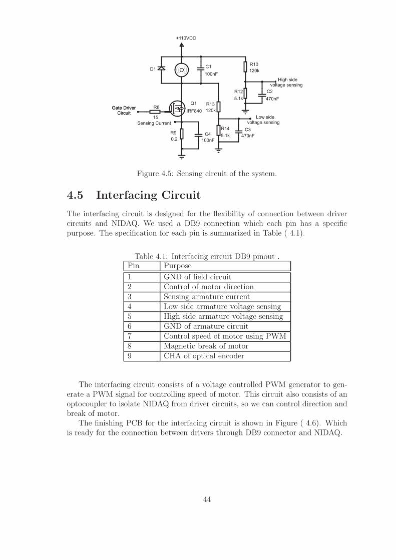
+110VDC

D1C1

100nF120k

R10

R12

5.1k

C2

470nF

C3

470nF

R14

5.1kC4

100nF0.2

R9

120k

R13R8

15

Q1

IRF840Gate Driver

CircuitGate Driver

Circuit

Sensing Current

Low sidevoltage sensing

High sidevoltage sensing

Figure 4.5: Sensing circuit of the system.

4.5 Interfacing Circuit

The interfacing circuit is designed for the flexibility of connection between drivercircuits and NIDAQ. We used a DB9 connection which each pin has a specificpurpose. The specification for each pin is summarized in Table ( 4.1).

Table 4.1: Interfacing circuit DB9 pinout .Pin Purpose

1 GND of field circuit2 Control of motor direction3 Sensing armature current4 Low side armature voltage sensing5 High side armature voltage sensing6 GND of armature circuit7 Control speed of motor using PWM8 Magnetic break of motor9 CHA of optical encoder

The interfacing circuit consists of a voltage controlled PWM generator to gen-erate a PWM signal for controlling speed of motor. This circuit also consists of anoptocoupler to isolate NIDAQ from driver circuits, so we can control direction andbreak of motor.

The finishing PCB for the interfacing circuit is shown in Figure ( 4.6). Whichis ready for the connection between drivers through DB9 connector and NIDAQ.

44

Figure 4.6: PCB of interfacing circuit

4.6 Data Acquisition

The data acquisition used in the thesis is the national instruments USB-6008. TheNational Instruments USB-6008 is a low-cost, multifunction data acquisition device(DAQ). It has 8 analog inputs, 2 analog outputs, and 12 digital input/outputs. Thedigital channels are divided into two ports. When one or more channels on eachport is set to either input or output, the port is locked into that particular mode.

The USB-6008 uses the NI-DAQmx driver software and is compatible withLabVIEW, Measurement Studio for Visual Studio, .NET, LabWindows/CVI, andMATLAB (version R2006a and newer). The image of this device is shown in Figure( 4.7).

Figure 4.7: The National Instruments USB-6008

NI DAQ USB-6008 which is available in control laboratories is used to applythe parameters identification analysis in MATLAB using DAQ toolbox. The spec-ifications for connections to NI DAQ was summarized in table 4.2.

For analysis, processing data and perform parameters identification on signalswe used Data Acquisition Toolbox (DAT) of MATLAB. Data Acquisition Toolboxsoftware provides a complete set of tools for analog input, analog output, anddigital I/O from a variety of PC-compatible data acquisition hardware. The toolboxlets you configure your external hardware devices, read data into MATLAB andSimulink environments for immediate analysis, and send out data.

45

Table 4.2: NI DAQ inputs and outputs.Channel Mode Purpose

Analog 0 (AI0) Differential input measuring voltage atmotor terminals

Analog 1 (AI1) Differential input measuring currentflowing in motor

Analog 2 (AI2) Differential input count # of pluses fromoptical encoder

Analog 0 (AO0) Differential output controlling speed ofmotor

Digital pin P0.0 Digital output mode controlling directionof motor

Digital pin P0.1 Digital output mode controlling break ofmotor

Data Acquisition Toolbox enables you to customize your acquisitions, access thebuilt-in features of hardware devices, and incorporate the analysis and visualizationfeatures of MATLAB and related toolboxes into your design. You can analyze orvisualize your data, save it for post-processing, and make iterative updates to yourtest setup based on your analysis results. Data Acquisition Toolbox allows youto use MATLAB as a single, integrated environment to support the entire dataacquisition, data analysis, and application development process.

Data Acquisition Toolbox also supports Simulink with blocks that enable you toincorporate live data or hardware configuration directly into Simulink models [33].You can then verify and validate your model against live, measured data as part ofthe system development process.

The measured voltage, current and speed of dc motor is plotted using MATLABbut there are some ripple noise due to switching of MOSFET and EMI effects, sowe design a digital average filter which it helps to reduce the effects of these noise.

4.7 Parameters Identification

This method is built in Simulink Parameter Estimation software in MATLAB forthe parameters identification of the dc motor. Simulink Parameter Estimation soft-ware is a simulink-based product for estimating and calibrating model parametersfrom experimental data. This product supports the following types of estimation:

• Transient Estimation : Estimate parameters by comparing model output tothe experimental data for a given input.

46

• Initial Condition Estimation : Estimate the initial conditions of states usingexperimental data.

• Adaptive Lookup Tables : Estimate the table values at the prescribed break-points by using measurements from the physical system.

Simulink Parameter Estimation software provides the tools used to:

1. Set up the problem.

2. Specify which model parameters to estimate.

3. Import and prepare the experimental data for parameter estimation (or pre-process).

4. View the estimation progress.

5. Validate the estimation results based on plots of measured versus. simulateddata and residuals.

How Simulink Parameter Estimation Software Works

Simulink Parameter Estimation software compares empirical data with data gener-ated by a Simulink model. Using optimization techniques, the software estimatesthe parameter and (optionally) initial conditions of states such that a user-selectedcost function is minimized. The cost function typically calculates a least-squareerror between the empirical and model data signals.

After you build a Simulink model, follow these steps to configure and run aparameter estimation:

1. Select Tools → Parameter Estimation in your Simulink model window.

This opens the Control and Estimation Tools Manager, creates a new project,and adds an Estimation node to the workspace directory tree.

2. Import the input and output data set for estimating parameters of yourSimulink model.

3. Select the parameters and initial conditions you want to estimate.

4. Configure the estimation itself, including cost functions and data views.

5. Run the estimation.

6. Check the results by examining either the cost-function values, plots, or pa-rameter values.

47

Description of the DC Motor System

We developed the model of the DC motor using simulink as discussed in chapter2. The model consists of input port for acquiring input signal of armature voltageand the output port for acquiring the output signals of armature current and speedof motor’s rotor. The model is shown in Figure ( 4.8)

Figure 4.8: Block diagram of DC motor

While manufacturers may provide values for some of these quantities, they areonly estimates. We want to estimate these parameters as precisely as possible forour model to ascertain whether it is an accurate representation of the actual DCmotor system.

When we apply a step voltage to the motor input, the motor shaft turns inresponse. However, if the model parameters do not match those of the physicalsystem, the model response will not match that of the actual system, either. Fig-ure 4.10 shows the current response of our model using the initial parameter valuesin the model with the armature input voltage shown if Figure 4.9. It is obvious thatwe need to estimate our parameters. This is where Simulink Parameter Estimationplays a pivotal role.

Estimating Parameters of the DC Motor Model

parameter estimation process consists of a number of well-defined steps:

• Collect test data from your system (experiment).

• Specify the parameters to estimate (including initial guesses, parameter bounds,etc.).

48

0 2 4 6 8 100

20

40

60

80

100

120

sec

Vol

ts

Armature Voltage

Armature Voltage

Figure 4.9: Armature voltage

• Configure our estimation and run a suitable estimation algorithm.

• Validate the results against other test data sets and repeat above steps ifnecessary.

Simulink Parameter Estimation provides a graphical user interface (GUI) tohelp you follow these steps, neatly organize your estimation project, and save it forfuture work. You can launch this product from the Tools menu of your Simulinkmodel. The tool automatically creates a default estimation project for you:

1. Importing Experimental Data: The first step in our estimation project is toimport the experimental data that we have collected from the actual DC mo-tor system. We imported two data sets corresponding to various experimentalconditions.

Simulink Parameter Estimation provides preprocessing tools such as noisefiltering, detrending, splitting, and so forth to prepare data sets for estima-tion and/or validation. You can import experimental data sets from vari-ous sources including MATLAB variables, MAT files, Excel files, or comma-separated-value files. Once you import the data, you can also plot them toconfirm that you have the right data sets in your estimation project.

2. Selecting Parameters for Estimation: Next, we select the model parameterswhose value we want to estimate. The tool automatically recognizes all theparameters that we use in the model and lets us select a subset of themfor estimation. Once we select the estimation parameters, we can set initialguesses for the parameter values, as well as the minimum and maximumbounds on these values, as shown below.

49

0 2 4 6 8 100

1

2

3

4

5

6

7

8

9

10

sec

Am

ps

Armature Current

Armature Current

Figure 4.10: Armature current response

Simulink Parameter Estimation lets you estimate some or all of these param-eters in a manner that best suits your application. For our DC motor, wewill estimate all six parameters of the motor model: B, J, Ke, Kt, La, and Ra

(these parameters are summarized in Table 2.1.

Figure 4.11: Selecting Parameters for Estimation

3. Defining an Estimation: Once we import our data and select the parametersto estimate, the next step is to create an estimation node in the GUI treeand configure various options. Each estimation uses your experimental data

50

sets to estimate the parameter that we have selected. However, we have theoption of using only some of the data sets for estimation while keeping theothers for validation. You can also select to estimate only a subset of theselected parameters.

Simulink Parameter Estimation also provides various state-of-the-art estima-tion algorithms. The most common selections include the nonlinear least-squares and Nelder-Mead optimization methods.

In our thesis we used the nonlinear least-square method and pattern searchalgorithm. Because it gives us a suitable results may be identical to the actualresponse and to compare them.

4. Optimization Options: Specify termination options in the Optimization op-tions area is a vital role in identification results. These options are shown inFigure 4.12.

Figure 4.12: Optimization options

These options define when the optimization terminates, these options are:

• Diff max change: The maximum allowable change in variables for finite-difference derivatives, we use the default value (0.1).

• Diff min change: The minimum allowable change in variables for finite-difference derivatives, we use the default value (1e-8).

• Parameter tolerance: Optimization terminates when successive param-eter values change by less than this number, we use the default value(1e-6).

• Maximum fun evals: The maximum number of cost function evaluationsallowed. The optimization terminates when the number of function eval-uations exceeds this value, we use the default value (400).

• Maximum iterations: The maximum number of iterations allowed. Theoptimization terminates when the number of iterations exceeds this value,we use the default value (100).

51

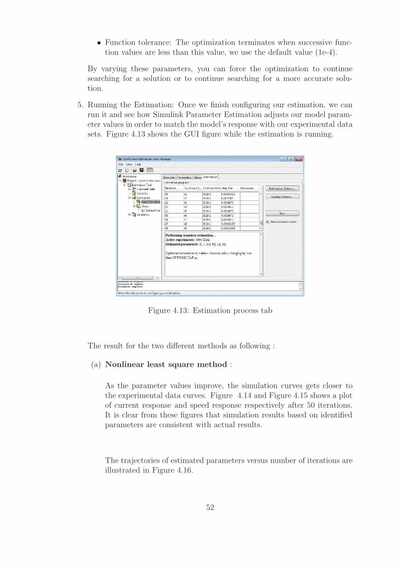
• Function tolerance: The optimization terminates when successive func-tion values are less than this value, we use the default value (1e-4).

By varying these parameters, you can force the optimization to continuesearching for a solution or to continue searching for a more accurate solu-tion.

5. Running the Estimation: Once we finish configuring our estimation, we canrun it and see how Simulink Parameter Estimation adjusts our model param-eter values in order to match the model’s response with our experimental datasets. Figure 4.13 shows the GUI figure while the estimation is running.

Figure 4.13: Estimation process tab

The result for the two different methods as following :

(a) Nonlinear least square method :

As the parameter values improve, the simulation curves gets closer tothe experimental data curves. Figure 4.14 and Figure 4.15 shows a plotof current response and speed response respectively after 50 iterations.It is clear from these figures that simulation results based on identifiedparameters are consistent with actual results.

The trajectories of estimated parameters versus number of iterations areillustrated in Figure 4.16.

52

0 2 4 6 8 100

1

2

3

4

5

6

7

8

9Current response

Am

p

sec

Actual current responseEstimated current reponse

Figure 4.14: Current response for the actual and estimated models

Comparing the response of the system before and after the estima-tion process clearly shows that the estimation successfully identified themodel parameters and the simulated response accurately matches theexperimental data. Also the speed response for the actual model of theDC motor is nearly identical to the estimated speed response as shownbelow.

Once the estimation is complete, we can inspect the estimated parametervalues. The Value column below displays the new parameter values atthe end of the estimation as illustrated in Figure 4.17.

When the algorithm is begin then the MATLAB workspace is begin toshow us the iteration process through identification. Below is a sampleof the estimation process. Table 4.3 summarized the estimation process.

A summary of the parameters estimation results are given in the tablebelow.

I’s clear from the table that nonlinear-least squares algorithm is powerfuland accurate because there are a very good match between the actualresponse and the estimated response for both current response and speedresponse for repeating the algorithm many times.

(b) Pattern search algorithm :

In this method we need to make so modifications on Matlab code inorder to apply this method. We change the following line

53

0 2 4 6 8 100

200

400

600

800

1000

1200

1400

1600

1800

2000

Actual speed responseEstimated speed reponse

Figure 4.15: Speed response for the actual and estimated models

hEst.OptimOptions.Algorithm = ’lsqnonlin’;

with this one

hEst.OptimOptions.Algorithm= ’Pattern’;.

When the algorithm is begin then the MATLAB workspace is begin toshow us the iteration process through identification. Below is a sampleof the estimation process. Table 4.5 summarized the estimation process.

After the iteration is finished we have a summary of the parametersestimation results which are given in Table 4.6.

It can be seen from Table 4.5 that we achieve the same results when weapply the method three times. This conclude that this method give usthe same results for the same acquiring signals.

Figure 4.18 and Figure 4.19 shows a plot of current response and speedresponse respectively. It is clear from these figures that simulation resultsbased on identified parameters are consistent with actual results.

The transfer function of the dc motor model is needed for studying the stateof our system and applying the controlling techniques on it. The transferfunction for current to voltage and speed to voltage is derived by using acode in MATLAB. These transfer functions are described as below from thenonlinear least square method:

54

0

0.01

0.02

B

0

0.05

0.1

J

0

1

2

Ke

0

1

2

Kt

0

0.5

1

La

0 5 10 15 20 25 30 35 40 45 500

10

20

Ra

Trajectories of Estimated Parameters

Iterations

Par

amet

er V

alue

s

Figure 4.16: Trajectories of estimated parameters

Ia(s)

V (s)=

s+ 1.039

0.01324s2 + 3.278s+ 80.75(4.2)

W (s)

V (s)=

65.04

0.01324s2 + 3.278s+ 80.75(4.3)

4.7.1 GUI Interface

GUI interface is implemented to automate the identification process. We build itusing matlab guide as illustrated in Fig. 4.20. It’s featured with all functions neededfor the identification process. These functions are:

1. Acquiring data: The function of this button is to apply a constant voltageabout 110V to the motor and acquires the armature voltage, armature currentand motor speed signals.

2. Parameters identification: The function of this button is to apply the suit-able algorithm (nonlinear least square) which is described above in simulinkparameter estimation but as matlab code.

3. Validation: The function of this button is to acquire a new data for validationthen comparing of estimated response to the actual repousse is plotted toshow how accuracy and efficiency of the estimated parameters. The mainparameters need for identification process is also displayed in the figure toparameters name.

The GUI interface is built for user friendly and to get all parameters at a mini-mum time. It providing control functions for speed controlling, direction controlling

55

Figure 4.17: Parameters estimation results

and stopping the motion of motor. An indication in the figure help us to know thedirection of motor is running.

56

Table 4.3: Summary of parameter estimation process(NLS method)Iter Func-

countf(x) Norm of

stepFirst-orderoptimality

CG-iterations

0 1 3043.05 3.59e+61 2 1377.92 0.0887085 3.36e+4 02 3 1195.33 0.456647 2.38e+5 03 4 1175.86 0.0234237 1.32e+4 04 5 1169.95 0.0888268 4.85e+4 05 6 1168.02 0.0105985 4.71e+3 06 7 1167.34 0.0289562 1.62e+4 07 8 1167.1 0.00419732 1.79e+3 0... ... ... ... ... ...... ... ... ... ... ...26 27 1166.96 5.82921e-6 28.3 027 28 1166.96 5.82921e-6 12.6 028 29 1166.96 1.4573e-6 1.25 029 30 1166.96 1.4573e-6 33.3 0

Table 4.4: Summary of parameter estimation results(NLS method)Parameters 1st case: 2nd case: 3rd case:

B(Nms) 0.019 0.019 0.019J(kg.m2) 0.01829 0.01829 0.01829Ke(V/rad/sec) 1.1895 1.1895 1.1895Kt(N.m/A) 1.1895 1.1895 1.1895La(H) 0.013242 0.013242 0.013242Ra(Ω) 3.2645 3.2645 3.2645

Table 4.5: Summary of parameter estimation process(Pattern method)Iter f-count f(x) MeshSize Method

0 1 3043.05 11 6 3043.05 0.5 Refine Mesh2 12 3043.05 0.25 Refine Mesh3 18 3043.05 0.125 Refine Mesh4 26 3043.05 0.0625 Refine Mesh5 33 2867.84 0.125 Successful Poll6 40 2867.84 0.0625 Refine Mesh... ... ... ... ...... ... ... ... ...48 387 1182.95 0.0002441 Refine Mesh49 399 1182.95 0.0001221 Refine Mesh50 400 1182.95 6.104e-005 Refine Mesh

57

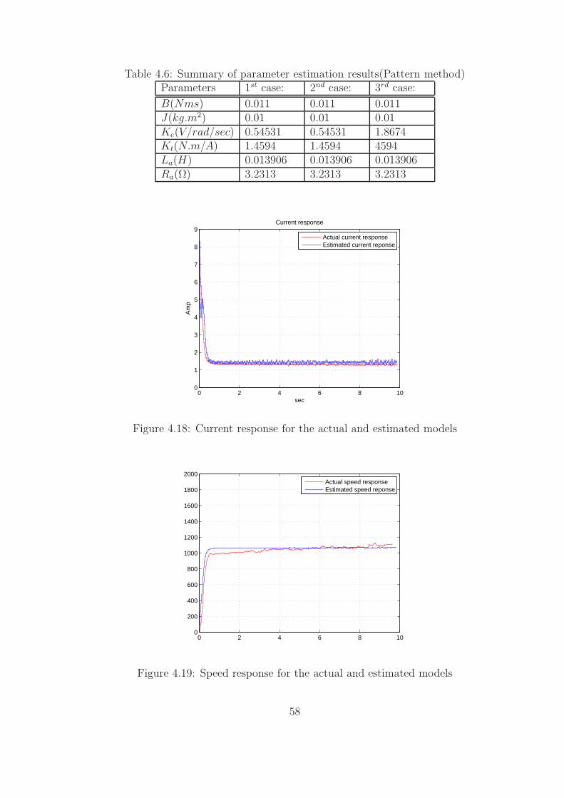
Table 4.6: Summary of parameter estimation results(Pattern method)Parameters 1st case: 2nd case: 3rd case:

B(Nms) 0.011 0.011 0.011J(kg.m2) 0.01 0.01 0.01Ke(V/rad/sec) 0.54531 0.54531 1.8674Kt(N.m/A) 1.4594 1.4594 4594La(H) 0.013906 0.013906 0.013906Ra(Ω) 3.2313 3.2313 3.2313

0 2 4 6 8 100

1

2

3

4

5

6

7

8

9Current response

Am

p

sec

Actual current responseEstimated current reponse

Figure 4.18: Current response for the actual and estimated models

0 2 4 6 8 100

200

400

600

800

1000

1200

1400

1600

1800

2000

Actual speed responseEstimated speed reponse

Figure 4.19: Speed response for the actual and estimated models

58

Main

Start motor Stop motor Change Dir.

Parameters Identification ofa Permanent Magnet DC Motor

Parameters

B

J

Ke

Kt

La

Ra

Acquiring Data

Parameters Iden.

Validation

Exit

Motor speed

Armature current

Armature voltage

Speed control

Figure 4.20: GUI interface

59

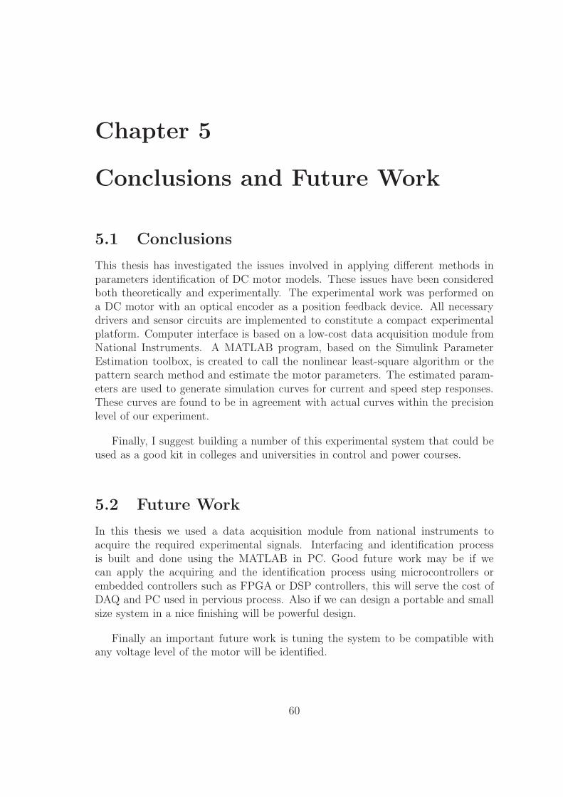
Chapter 5

Conclusions and Future Work

5.1 Conclusions

This thesis has investigated the issues involved in applying different methods inparameters identification of DC motor models. These issues have been consideredboth theoretically and experimentally. The experimental work was performed ona DC motor with an optical encoder as a position feedback device. All necessarydrivers and sensor circuits are implemented to constitute a compact experimentalplatform. Computer interface is based on a low-cost data acquisition module fromNational Instruments. A MATLAB program, based on the Simulink ParameterEstimation toolbox, is created to call the nonlinear least-square algorithm or thepattern search method and estimate the motor parameters. The estimated param-eters are used to generate simulation curves for current and speed step responses.These curves are found to be in agreement with actual curves within the precisionlevel of our experiment.

Finally, I suggest building a number of this experimental system that could beused as a good kit in colleges and universities in control and power courses.

5.2 Future Work

In this thesis we used a data acquisition module from national instruments toacquire the required experimental signals. Interfacing and identification processis built and done using the MATLAB in PC. Good future work may be if wecan apply the acquiring and the identification process using microcontrollers orembedded controllers such as FPGA or DSP controllers, this will serve the cost ofDAQ and PC used in pervious process. Also if we can design a portable and smallsize system in a nice finishing will be powerful design.

Finally an important future work is tuning the system to be compatible withany voltage level of the motor will be identified.

60

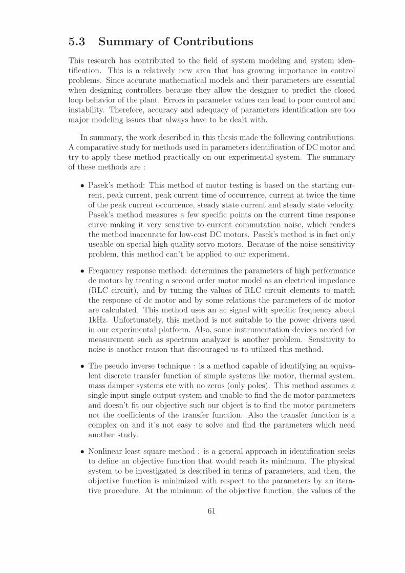
5.3 Summary of Contributions

This research has contributed to the field of system modeling and system iden-tification. This is a relatively new area that has growing importance in controlproblems. Since accurate mathematical models and their parameters are essentialwhen designing controllers because they allow the designer to predict the closedloop behavior of the plant. Errors in parameter values can lead to poor control andinstability. Therefore, accuracy and adequacy of parameters identification are toomajor modeling issues that always have to be dealt with.

In summary, the work described in this thesis made the following contributions:A comparative study for methods used in parameters identification of DCmotor andtry to apply these method practically on our experimental system. The summaryof these methods are :

• Pasek’s method: This method of motor testing is based on the starting cur-rent, peak current, peak current time of occurrence, current at twice the timeof the peak current occurrence, steady state current and steady state velocity.Pasek’s method measures a few specific points on the current time responsecurve making it very sensitive to current commutation noise, which rendersthe method inaccurate for low-cost DC motors. Pasek’s method is in fact onlyuseable on special high quality servo motors. Because of the noise sensitivityproblem, this method can’t be applied to our experiment.

• Frequency response method: determines the parameters of high performancedc motors by treating a second order motor model as an electrical impedance(RLC circuit), and by tuning the values of RLC circuit elements to matchthe response of dc motor and by some relations the parameters of dc motorare calculated. This method uses an ac signal with specific frequency about1kHz. Unfortunately, this method is not suitable to the power drivers usedin our experimental platform. Also, some instrumentation devices needed formeasurement such as spectrum analyzer is another problem. Sensitivity tonoise is another reason that discouraged us to utilized this method.

• The pseudo inverse technique : is a method capable of identifying an equiva-lent discrete transfer function of simple systems like motor, thermal system,mass damper systems etc with no zeros (only poles). This method assumes asingle input single output system and unable to find the dc motor parametersand doesn’t fit our objective such our object is to find the motor parametersnot the coefficients of the transfer function. Also the transfer function is acomplex on and it’s not easy to solve and find the parameters which needanother study.

• Nonlinear least square method : is a general approach in identification seeksto define an objective function that would reach its minimum. The physicalsystem to be investigated is described in terms of parameters, and then, theobjective function is minimized with respect to the parameters by an itera-tive procedure. At the minimum of the objective function, the values of the

61

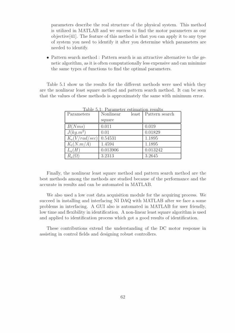
parameters describe the real structure of the physical system. This methodis utilized in MATLAB and we success to find the motor parameters as ourobjective[41]. The feature of this method is that you can apply it to any typeof system you need to identify it after you determine which parameters areneeded to identify.

• Pattern search method : Pattern search is an attractive alternative to the ge-netic algorithm, as it is often computationally less expensive and can minimizethe same types of functions to find the optimal parameters.

Table 5.1 show us the results for the different methods were used which theyare the nonlinear least square method and pattern search method. It can be seenthat the values of these methods is approximately the same with minimum error.

Table 5.1: Parameter estimation resultsParameters Nonlinear least

squarePattern search

B(Nms) 0.011 0.019J(kg.m2) 0.01 0.01829Ke(V/rad/sec) 0.54531 1.1895Kt(N.m/A) 1.4594 1.1895La(H) 0.013906 0.013242Ra(Ω) 3.2313 3.2645

Finally, the nonlinear least square method and pattern search method are thebest methods among the methods are studied because of the performance and theaccurate in results and can be automated in MATLAB.

We also used a low cost data acquisition module for the acquiring process. Wesucceed in installing and interfacing NI DAQ with MATLAB after we face a someproblems in interfacing. A GUI also is automated in MATLAB for user friendly,low time and flexibility in identification. A non-linear least square algorithm is usedand applied to identification process which got a good results of identification.

These contributions extend the understanding of the DC motor response inassisting in control fields and designing robust controllers.

62

Bibliography

[1] N. Sinha, C. Dicenzo and B. Szabados, “ Modeling of DC motors for control ap-plications ”. IEEE Trans. Industrial Electronics And Control Instrumentation,vol. IECI-21, pp. 84-88, August 1974.

[2] W. Lord and J. Hwang, “ DC servomotors modeling and parameter determina-tion ”. IEEE Trans. Industrial Applications, vol. IA-3, pp. 234-243, May/June1973.

[3] W. Lord and J. Hwang, “ DC motor model parameters ”. IEEE Trans. onIndustrial Electronics and Control Instrumentation, vol. IECI-23, No.3, August1975.

[4] R. Schulz, “A frequency for determining the parameters of high performanceDC motors”. IEEE Trans. on Industrial Electronics, vol. IE-30, No.1, Februray1983.

[5] A. Rajkumar and R. Somanahtham, “ Determination of DC motor transientsusing a microcomputer ”. IEEE Trans, on Instrumentaion and Measurement,vol. 37, No.4, Dec. 1988.

[6] S. Weerasooriya and M. El-Sharkawi, “ Identification and control of a DC mo-tor using back-propagation neural networks ”. IEEE Trans. on Energy Con-version, vol. 6, No.4, December 1991.

[7] Y. G. Jung, K. Cho, Y. Lim, J. Park and Y. H. Change, “ Time domainidentification of brushless DC motor parameters ”. IEEE Trans. on IndustrialElectronics, vol. 2, 593-597, Februray 1992.

[8] D. M. Gillard and K. E. Bollinger, “ Neural network identification of powersystem transfer functions ”. IEEE Transactions on Energy Conversion, Vol.11, No. 1, March 1996.

[9] D. M. Gillard and K. E. Bollinger, “ Online identification and control of aDC motor using learning adaptation of neural networks ”. IEEE Trans. onIndustrial Applications, VOL. 36, NO. 3, MAY/JUNE 2000.

[10] Hanamoto, T. Tanaka, Y. Karube, I. Mochizuk and T. Xu, Z., “ A pa-rameter estimation method using block pulse functions for DC servo motor

63

systems”. Industrial Electronics, Control, Instrumentation, and Automation,1992. Power Electronics and Motion Control, proceedings of the 1992 Interna-tional Conference on vol., no., pp.1288-1293 vol.3, 9-13 Nov 1992.

[11] S. Saab and R. Abi Kaed-Bey, “ Parameter identification of a DC motor: anexperimetnal approach ”. IEEE Trans. on Electronics, Circuits and Systems,vol. 2, 981-984, 2001.

[12] A. Dupuis, M. Ghribi and A. Kaddouri, “ Multiobjective genetic estimation ofDC motor parameters and load torque ”. IEEE International Conference onIndustrial Technology, vol. 3, 1511-1514, Dec. 2004.

[13] Radojka Krneta, Sanja Antic and Danilo Stojanovic, “ Recursive least squaresmethod in parameters identification of DC motors models ”. ELEC. ENERG,vol. 18, no. 3, 467-478, December 2005.

[14] R. Garrido and R. Miranda, “ Closed loop identification of a DC servomecha-nism ”. Power Electronics Congress, 10th IEEE, vol., no., pp.1-5, 16-18 Oct.2006.

[15] W. P. Aung, “ Analysis on modeling and simulink of DC motor and its drivingsystem used for wheeled mobile robot ”. International Journal of Computer,Information, and Systems Science, and Engineering, Volume 2 Number 1, Nov.2007.

[16] M. Hadef and R. Mekideche, “ Parameter identification of a separately excitedDC motor via inverse problem methodology ”. Turk J Elec Eng and Comp Sci,vol. 17, No.2, 2009.

[17] Adrian V. Bos, Parmaeter Estimation for Scientists and Engineers, First Edi-tion, Wiley, Inc., 2007.

[18] Rik Pintelon and Johan Schoukens, System identification: a frequency domainapproach, First Edition, IEEE Press, Inc., 2001.

[19] Wikipedia, The free encyclopedia http://en.wikipedia.org/wiki/Electric motor

[20] Ogata K., Modern Control Engineering , 2nd ed., Prentice Hall, NJ, 1990.

[21] Kuo B.C., Automatic Control Systems, 6th ed., Prentice Hall, NJ, 1991.

[22] DC Servomotors Tutorial, Callon Technology, URL:http://www.callantechnology.com/callan technology resources/

[23] Genetic Algorithm and Direct Search Toolbox, Mathworks, URL:http://www.mathworks.com/access/helpdesk/help/toolbox/gads/f7805.html

[24] Paul Scherz, Practical Electronics For Inventors, First Edition, McGraw-Hill,Inc., 2000.

64

[25] Selecting the right MOSFET driver, Hearst Electronic Products,URL:http://www2.electronicproducts.com/Selecting the right MOSFET driver-article-microchip-mar2007-html.aspx.

[26] Motor Control Sensor Feedback Circuits, Microchip, Inc.URL:http://ww1.microchip.com/downloads/en/AppNotes/00894a.pdf.

[27] Kuo B., Digital Control Systems, Holt Saunders, Tokyo, 1980.

[28] Ogata K., Discrete-Time Control Systems, Prentice Hall, N.J, 1987.

[29] Astrom K.J., Wittenmark B., Computer Controlled Systems - Theory andDesign. 3rd edition, Prentice-Hall, Englewood Cliffs. N.J., 1997.

[30] Franklin G.F., Powell J.D., Workman M.L., Digital Control of Dynamic Sys-tems, 3rd edition, Addison Wesley, Reading, Mass, 1998.

[31] Thomas L. Floyd, Electronics Fundamentals: Circuits, Devices and Applica-tions, Prentice Hall, 7th Ed., 2006.

[32] NI USB-6008, National Instruments Corporation,URL:http://sine.ni.com/nips/cds/view/p/lang/en/nid/14604.

[33] Data Acquisition Toolbox, The MathWorks, Inc.URL:http://www.mathworks.com/products/daq/.

[34] Franklin G., Powell J.D., Feedback Control of Dynamic Systems, AddisonWesley, Reading, Mass, 1986.

[35] Shinskey F.G., Process Control Systems, McGraw-Hill, N.Y., 1979.

[36] Wirk G.S., Digital Computer Systems, MacMillan, London, 1991.

[37] Loan D. Landau, Gianluca Zito, Digital Control Systems - design, identificationand implementation, Springer Verlag, London, 2006.

[38] Phillips C.L., Nagle H.T., Digital Control Systems Analysis and Design, 3rdedition. Prenctice Hall, N.J., 1995.

[39] Richard C. Dorf, Robert H. Bishop, Modern Control Systems, Addison Wesely,2002.

[40] Gene F. Franklin, J. David Powell, Abbas Emami-Naeini, Feedback ControlOf Dynamic Systems, 5th ed., New Jersy, Prentice Hall, 2006.

[41] M. Salah and M. Abdelati, “ Parameters identification of a permanent magnetDC motor ”. Modelling, Identification and Control MIC, 675-085 , February2010.

65

Appendix A

MALTLAB Codes

A.1 Acquiring Signals

%%%%%%%%%%%%%%%%%%%%%%%%%%%%%%%%%%%%%%%%%%%% File: acq but.m% Usage: Interfacing with NI-DAQ6008 to send as anlaog output signal to run% DC motor for acquiring analog signals for 10 sec’s of time.% Author: Eng. Mohammed S. Salah% http://www.ucas.edu.ps% Department of electrical engineering% The Islamic University of Gaza% May 2009%%%%%%%%%%%%%%%%%%%%%%%%%%%%%%%%%%%%%%%%%%%global arm volt avgglobal sen cur avgglobal time

clcscalevolt=132.1/5.1; scalecurrent=22.4; Vt=110; Vpwm=Vt/25;%%%%%%%%%%%%%%%%%%%%%%%%%%%%%%%%%%%%%delete open daqsopenDAQ = daqfind;for i = 1:length(openDAQ)

delete(openDAQ(i));end

% open the daq%%%%%%%%%%%%%%%%%%%%%%%%%configure analog inputsai = analoginput(’Nidaq’,’Dev1’);

66

chan = addchannel(ai,0:2);

%%%%%%%%%%%%%%%%%%%%%%%%% configure analog outputsdio = digitalio(’nidaq’,’Dev1’);addline(dio,0,0,’out’);

ao = analogoutput(’nidaq’,’Dev1’);ch = addchannel(ao, 0);putsample(ao,0); %%% stop motor at default

warning(’off’, ’all’)button = questdlg(’Turn on the power and press OK button to begin acquir-ing’,’Acquiring data’,’Ok’,’Cancel’,’No’);

switch buttoncase ’Ok’,

set(handles.ind1,’String’,’Begin’)set(handles.ind1,’Visible’,’on’)

Fs=3300 %% sampling rate 1000 samples/secset(ai,’samplespertrigger’,Inf);% set sample rate

set(ai,’samplerate’,Fs); %Fastest sampling by USB-6008

set(ai,’loggingmode’,’disk’); % set to log to file

%%%%%%%%

%%%%%start(ai)% start data collection

putsample(ao,Vpwm); %%% start motor

message = ’begin data aquisition for 10 secs’% report when finished

pause(10)

stop(ai)% stop data collection

putsample(ao,0); %%% stop motor at defaultmessage = ’data aquisition finished’% report when finished

%%%%%%%%%%%%%%%%%%%%%%%%%%%%%%%%%%%%%%%%%

clear message

67

% get data from log file

file = get(ai,’logfilename’);

[data,time] = daqread(file);

arm volt=data(:,1);sen cur=data(:,2);opti enc=data(:,3);

arm volt=arm volt.*scalevolt;sen cur=sen cur.*scalecurrent;

fs=Fs;Duration=.01; % seconds .01totalrpm=[];totaltt=[];% Start the acquisition.

% [orgdata time] = getdata(ai,ai.SamplesAcquired);orgdata=opti enc;%%%%%%%%%%%%%%%%%%%%%%%%%%%%%%%%%%%%%%%%%%%

% Set the threshold to 3.5 V.threshold = 2.4;

numsamples=length(orgdata);numofloops=round(numsamples/(fs*Duration))-1;

for k=0:numofloops-1

data=orgdata(1+k*fs*Duration:fs*Duration*(1+k));

% Create the offset data. Need to append a NaN to the final samplesince

% both vectors need to have the same length.offsetData = [data(2:end); NaN];

% Find the rising edge.risingEdge = find(data < threshold & offsetData > threshold);

% Find the falling edge.fallingEdge = find(data > threshold & offsetData < threshold);

if length(time(risingEdge))==0

68

numPulses=0;%disp(’no pulses’)

else%plot(time(risingEdge), threshold, ’rx’);

numPulses = length(risingEdge);%disp([’numPulse = ’,num2str(numPulses)])

end%%%%%%%%%%%% Compute the speed rpm%%%%%%%%%%%%%%%rpm=(60/Duration)*numPulses/120*2.5; % 120 is num of slits of disk

totalrpm=[totalrpm rpm];totaltt=[totaltt k*Duration];

end%%%%%%%%%%%%%%%%%%%%%%%%%%%%%

helpdlg(’Acquiring data is finished, turn off motor’,’Acquiring data’);

%%%%%%%% processing data for identification%%%%%%%%%%%%%%% average filter fro%%%%%%%%%%%%%%% armature voltageM=30;a=[1 zeros(1,length(M))];b=(1/M)*[ones(1,M)];arm volt avg=filter(b,a,arm volt);

%%%%%%%%%%%%%% armature currentM=30;a=[1 zeros(1,length(M))];b=(1/M)*[ones(1,M)];sen cur avg=filter(b,a,sen cur);%%% speedM=20;a=[1 zeros(1,length(M))];b=(1/M)*[ones(1,M)];totalrpm avg=filter(b,a,totalrpm);

totalrpm avg sim=[0 totalrpm(21:end)];totaltt sim=totaltt(1:end-19);

M=20;a=[1 zeros(1,length(M))];b=(1/M)*[ones(1,M)];

69

totalrpm avg sim=filter(b,a,totalrpm avg sim);%%%%%%%%%%%%%%%%%%%%%%%%%% Voltage === current model

signals = struct(’values’,totalrpm avg sim’,’dimesions’,1,’label’,”)Ws = struct(’time’,totaltt sim’,’signals’,signals,’blockName’,’Motor2/To

Workspace1’)

signals = struct(’values’,arm volt avg,’dimesions’,1,’label’,”);Vs = struct(’time’,time,’signals’,signals,’blockName’,’Motor2/To Workspace’);

signals = struct(’values’,sen cur avg,’dimesions’,1,’label’,”);Is = struct(’time’,time’,’signals’,signals,’blockName’,’Motor2/To Workspace1’);

save mydata.mat arm volt arm volt avg sen cur sen cur avg time to-taltt sim totalrpm avg sim Ws Vs Is

set(handles.pushbutton2,’Enable’,’on’)set(handles.pushbutton3,’Enable’,’on’)

set(handles.pushbutton6,’Enable’,’on’)set(handles.pushbutton7,’Enable’,’on’)set(handles.pushbutton8,’Enable’,’on’)

set(handles.ind1,’String’,’Ready’)set(handles.ind1,’Visible’,’on’)

end% collect data until a ’stop’ is issuedwarning(’on’, ’all’)

70

A.2 Parameters Identification

%%%%%%%%%%%%%%%%%%%%%%%%%%%%%%%%%%%%%%%%%%%% File: parm ident.m% Usage: Applying parameters identification which we used the nonlinear% least square method to find DC Motor parameters.% Author: Eng. Mohammed S. Salah% http://www.ucas.edu.ps% Department of electrical engineering% The Islamic University of Gaza% June 2009%%%%%%%%%%%%%%%%%%%%%%%%%%%%%%%%%%%%%%%%%%%global arm volt avgglobal sen cur avgglobal time

clcevalin(’base’,[’load mydata.mat’]);

Ws = evalin(’base’, ’Ws’);Vs = evalin(’base’, ’Vs’);Is = evalin(’base’, ’Is’);

J=0.01;B=0.01;Ke=0.1;Kt=0.1;Ra=.2;La=0.5;T=0;Fs=3300 %% sampling rate 1000 samples/secTs=1/Fs;%0.00001;Ia=[];W=[];

%%%%%%%%%%%%% data for parameter identification

iodata=[Vs.signals.values Is.signals.values];

save mydata1.mat J B Ke Kt Ra La T Fs Ts;evalin(’base’,[’load mydata1.mat’]);

model = ’spedcmotor model’;open system(model)set( find system(model, ’FindAll’, ’on’, ’BlockType’, ’Scope’), ’Open’, ’off’ )

hExp = ParameterEstimator.TransientExperiment(model);set(hExp.InputData(1), ’Data’, iodata(:,1), ’Time’, time);set(hExp.OutputData(1), ’Data’, iodata(:,2), ’Time’, time);

%%%%%%%%%%%%%%%%%%%%%%%%%%%%%%%hPar(1) = ParameterEstimator.Parameter(’B’);

71

set(hPar(1), ’Minimum’, 0, ’Maximum’, 10, ’Estimated’, true)

hPar(2) = ParameterEstimator.Parameter(’J’);set(hPar(2), ’Minimum’, 0, ’Maximum’, 10, ’Estimated’, true)

hPar(3) = ParameterEstimator.Parameter(’Ke’);set(hPar(3), ’Minimum’, 0, ’Maximum’, 10, ’Estimated’, true)

hPar(4) = ParameterEstimator.Parameter(’Kt’);set(hPar(4), ’Minimum’, 0, ’Maximum’, 10, ’Estimated’, true)

hPar(5) = ParameterEstimator.Parameter(’La’); % Initial value: Zd = -80set(hPar(5), ’Minimum’, 0, ’Maximum’, 10, ’Estimated’, true)

hPar(6) = ParameterEstimator.Parameter(’Ra’);set(hPar(6), ’Minimum’, 0, ’Maximum’, 100, ’Estimated’, true)

%%%%%%%%%%%%hEst = ParameterEstimator.Estimation(model, hPar, hExp);%%%%%%%%%%

hEst.OptimOptions.Algorithm= ’lsqnonlin’;hEst.OptimOptions.GradientType= ’basic’;hEst.OptimOptions.Display= ’iter’;

estimate(hEst)

find(hEst.Parameters, ’Estimated’, true)

B = evalin(’base’, ’B’);B=0.0201202;J = evalin(’base’, ’J’);Ke = evalin(’base’, ’Ke’);Kt = evalin(’base’, ’Kt’);La = evalin(’base’, ’La’);Ra = evalin(’base’, ’Ra’);

set(handles.B value,’String’,num2str(B))set(handles.J value,’String’,num2str(J))set(handles.Ke value,’String’,num2str(Ke))set(handles.Kt value,’String’,num2str(Kt))set(handles.La value,’String’,num2str(La))set(handles.Ra value,’String’,num2str(Ra))

72

A.3 Validation of Identification

%%%%%%%%%%%%%%%%%%%%%%%%%%%%%%%%%%%%%%%%%%%% File: validation.m% Usage: Get new date from DC motor using NI-DAQ6008 and make validation% between acutual response and estimated response.% Author: Eng. Mohammed S. Salah% http://www.ucas.edu.ps% Department of electrical engineering% The Islamic University of Gaza% July 2009%%%%%%%%%%%%%%%%%%%%%%%%%%%%%%%%%%%%%%%%%%%global arm volt avgglobal sen cur avgglobal time

clcevalin(’base’,[’load mydata.mat’]);

Ws = evalin(’base’, ’Ws’);Vs = evalin(’base’, ’Vs’);Is = evalin(’base’, ’Is’);

B= eval(get(handles.B value,’String’));J= eval(get(handles.J value,’String’));Ke= eval(get(handles.Ke value,’String’));Kt= eval(get(handles.Kt value,’String’));La= eval(get(handles.La value,’String’));Ra= eval(get(handles.Ra value,’String’));sen cur avg = evalin(’base’, ’sen cur avg’);

totalrpm avg sim = evalin(’base’, ’totalrpm avg sim’);totaltt sim = evalin(’base’, ’totaltt sim’);

%%%%%%%%%%%%% current transfer functionnumI=[1 B/J];denI=[La (Ra+La*B/J) (Ra*B/J+Ke*Kt/J)];%%disp(’current tranfer function’)Isys=tf(numI,denI);[ia1,t1]=lsim(Isys,Vs.signals.values,Vs.time);

sen cur mean=mean(sen cur avg(5000:end))current mean estimated=mean(ia1(end-20:end))err diff=sen cur mean-current mean estimated;while err diff>0.001

73

B=B+0.001;numI=[1 B/J];denI=[La (Ra+La*B/J) (Ra*B/J+Ke*Kt/J)];%%disp(’current tranfer function’)Isys=tf(numI,denI);[ia1,t1]=lsim(Isys,Vs.signals.values,Vs.time);

current mean estimated=mean(ia1(end-20:end));err diff=sen cur mean-current mean estimated;

endIsys=tf(numI,denI)set(handles.B value,’String’,num2str(B))figureplot(Is.time,Is.signals.values,’r’)

title(’Current response’)ylabel(’Amp’)xlabel(’sec’)gridhold onplot(t1,ia1);

legend(’Actual current response’,’Estimated current reponse’)

%%%%%%%%%%%% speed transfer functionnumW=[Kt/J];denW=[La (Ra+La*B/J) (Ra*B/J+Ke*Kt/J)];%%%disp(’speed tranfer function’)%subplot(2,1,2)Wsys=tf(numW,denW)[w2,t2]=lsim(Wsys,Vs.signals.values,Vs.time);figureplot(Ws.time,Ws.signals.values,’r’)hold onDuration=.01; % seconds .01totalrpm mean=mean(totalrpm avg sim(5/Duration:9/Duration));

speed mean estimated=mean(w2(end-20:end));correction=totalrpm mean/speed mean estimated;w2=correction*w2;gridplot(t2,w2);legend(’Actual speed response’,’Estimated speed reponse’)ylim([0 2000])

74

Appendix B

Schematics

75

Figure B.1: Field driver unit schematics.

76

Figure B.2: Field driver unit layout.

77

Figure B.3: Armature driver unit.

78

Figure B.4: Armature driver unit layout.

79

Figure B.5: Armature power circuit.

80

Figure B.6: Field power circuit.

81

Figure B.7: interfacing circuit.

82