Parallel Visualization on Large Clusters using MapReduceHuy T. Vo∗

SCI InstituteUniversity of Utah

Jonathan BronsonSCI Institute

University of Utah

Brian SummaSCI Institute

University of Utah

Joao L.D. CombaInstituto de Informatica

UFRGS, Brazil

Juliana FreireSCI Institute

University of Utah

Bill HoweeScience Institute

University of Washington

Valerio PascucciSCI Institute

University of Utah

Claudio T. SilvaSCI Institute

University of Utah

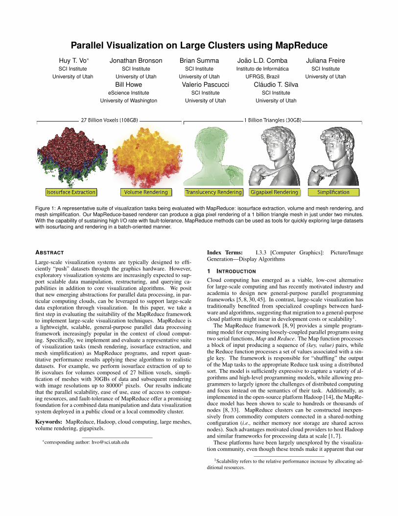
Figure 1: A representative suite of visualization tasks being evaluated with MapReduce: isosurface extraction, volume and mesh rendering, andmesh simplification. Our MapReduce-based renderer can produce a giga pixel rendering of a 1 billion triangle mesh in just under two minutes.With the capability of sustaining high I/O rate with fault-tolerance, MapReduce methods can be used as tools for quickly exploring large datasetswith isosurfacing and rendering in a batch-oriented manner.

ABSTRACT

Large-scale visualization systems are typically designed to effi-ciently “push” datasets through the graphics hardware. However,exploratory visualization systems are increasingly expected to sup-port scalable data manipulation, restructuring, and querying ca-pabilities in addition to core visualization algorithms. We positthat new emerging abstractions for parallel data processing, in par-ticular computing clouds, can be leveraged to support large-scaledata exploration through visualization. In this paper, we take afirst step in evaluating the suitability of the MapReduce frameworkto implement large-scale visualization techniques. MapReduce isa lightweight, scalable, general-purpose parallel data processingframework increasingly popular in the context of cloud comput-ing. Specifically, we implement and evaluate a representative suiteof visualization tasks (mesh rendering, isosurface extraction, andmesh simplification) as MapReduce programs, and report quan-titative performance results applying these algorithms to realisticdatasets. For example, we perform isosurface extraction of up tol6 isovalues for volumes composed of 27 billion voxels, simpli-fication of meshes with 30GBs of data and subsequent renderingwith image resolutions up to 800002 pixels. Our results indicatethat the parallel scalability, ease of use, ease of access to comput-ing resources, and fault-tolerance of MapReduce offer a promisingfoundation for a combined data manipulation and data visualizationsystem deployed in a public cloud or a local commodity cluster.

Keywords: MapReduce, Hadoop, cloud computing, large meshes,volume rendering, gigapixels.

∗corresponding author: hvo@sci.utah.edu

Index Terms: I.3.3 [Computer Graphics]: Picture/ImageGeneration—Display Algorithms

1 INTRODUCTION

Cloud computing has emerged as a viable, low-cost alternativefor large-scale computing and has recently motivated industry andacademia to design new general-purpose parallel programmingframeworks [5, 8, 30, 45]. In contrast, large-scale visualization hastraditionally benefited from specialized couplings between hard-ware and algorithms, suggesting that migration to a general-purposecloud platform might incur in development costs or scalability1.

The MapReduce framework [8, 9] provides a simple program-ming model for expressing loosely-coupled parallel programs usingtwo serial functions, Map and Reduce. The Map function processesa block of input producing a sequence of (key, value) pairs, whilethe Reduce function processes a set of values associated with a sin-gle key. The framework is responsible for “shuffling” the outputof the Map tasks to the appropriate Reduce task using a distributedsort. The model is sufficiently expressive to capture a variety of al-gorithms and high-level programming models, while allowing pro-grammers to largely ignore the challenges of distributed computingand focus instead on the semantics of their task. Additionally, asimplemented in the open-source platform Hadoop [14], the MapRe-duce model has been shown to scale to hundreds or thousands ofnodes [8, 33]. MapReduce clusters can be constructed inexpen-sively from commodity computers connected in a shared-nothingconfiguration (i.e., neither memory nor storage are shared acrossnodes). Such advantages motivated cloud providers to host Hadoopand similar frameworks for processing data at scale [1, 7].

These platforms have been largely unexplored by the visualiza-tion community, even though these trends make it apparent that our

1Scalability refers to the relative performance increase by allocating ad-ditional resources.

community must inquire into their viability for use in large-scale vi-sualization tasks. The conventional modus operandi of “throwingdatasets” through a (parallel) graphics pipeline relegates data ma-nipulation, conditioning, and restructuring tasks to an offline sys-tem and ignores their cost. As data volumes grow, these costs —especially the cost of transferring data between a storage cluster anda visualization cluster — begin to dominate. Cloud computing plat-forms thus open new opportunities in that they afford both general-purpose data processing as well as large-scale visualization.

In this paper, we take a step towards investigating the suitabil-ity of the cloud-based infrastructure for large-scale visualization.We observed that common visualization algorithms can be natu-rally expressed using the MapReduce abstraction with simple im-plementations that are highly scalable. We designed MapReduce-based algorithms for memory-intensive visualization techniques,and evaluated them with several experiments. Results indicate thatMapReduce offers a foundation for a combined storage, processing,analysis, and visualization system that is capable of keeping pacewith growth in data volume (attributable to scalability and fault-tolerance) as well as growth in application diversity (attributable toextensibility and ease of use). Figure 1 illustrates results for isosur-face extraction, volume and mesh rendering, and simplification.

In summary, the main contributions of the paper are:

• The design of scalable MapReduce-based algorithms for core,memory-intensive visualization techniques: mesh and volumerendering, isosurface extraction, and mesh simplification;

• An experimental evaluation of these algorithms using both amulti-tenant cloud environment and a local cluster;

• A discussion on the benefits and challenges of developing vi-sualization algorithms for the MapReduce model.

2 RELATED WORK

Recently, a new generation of systems have been introduced fordata management in the cloud, such as file systems [3, 23], storagesystems [6,10], and hosted DBMSs [29,42]. MapReduce [8,44] andsimilar massively parallel processing systems (e.g.,, Clustera [11],Dryad [20], and Hadoop [14]) along with their specialized lan-guages [5, 30, 45]) are having a great impact on data processing inthe cloud. Despite their benefits to other fields, these systems havenot yet been applied to scientific visualization.

One of the first remote visualization applications [39] uses theX Window System’s transport mechanism in combination with Vir-tual Network Computing (VNC) [34] to allow remote visualiza-tion across different platforms. IBM’s Deep Computing Visual-ization (DCV) system [18], SGI’s OpenGL Vizserver [37] and theChromium Renderserver (CRRS) [32] perform hardware acceler-ated rendering for OpenGL applications. A data management andvisualization system for managing finite element simulations inmaterials science, which uses Microsoft’s SQL Server databaseproduct coupled to IBM’s OpenDX visualization platform is de-scribed in [15]. Indexes provide efficient access to data subsets,and OpenDX renders the results into a manipulable scene allowinginspection of non-trivial simulation features such as crack propaga-tion. However, this architecture is unlikely to scale beyond a fewnodes due to its dependency on a conventional database system.

Another approach to distributed visualization is to provide accessto the virtual desktop on a remote computing system [18,24,32,37],such that data remains on the server and only images or graphicsprimitives are transmitted to the client. Systems like VisIt [24] andParaView [31] provide a scalable visualization and rendering back-end that sends images to a remote client. Many scientific communi-ties are creating shared repositories with increasingly large, curateddatasets [19, 27, 38]. To illustrate the scale of these projects, theLSST [27] is predicted to generate 30 terabytes of raw data per

DATA ON HDFS

INPUT PARTITION

SHUFFLING

SORT IN PARALLEL

OUTPUT PARTITION

DATA ON HDFS

MAP

REDUCE REDUCE

MAP MAP MAP

Figure 2: Data transfer and communication of a MapReduce job inHadoop. Data blocks are assigned to several Maps, which emit key/-value pairs that are shuffled and sorted in parallel. The Reduce stepemits one or more pairs, with results stored on the HDFS.

night for a total of 6 petabytes per year. Systems associated withthese repositories support only simple retrieval queries, leaving theuser to perform analysis and visualization independently.

3 MAPREDUCE OVERVIEW

MapReduce is a framework to process massive data on distributedsystems. It provides an abstraction that relies on two operations:

• Map: Given input, emit one or more (key, value) pairs.• Reduce: Process all values of a given key and emit one or more

(key, value) pairs.

A MapReduce job is composed of three phases: map, shuffle andreduce. Each dataset to be processed is partitioned into fixed-sizeblocks. In the map phase, each task processes a single block andemits zero or more (key, value) pairs. In the shuffle phase, the sys-tem sorts the output of the map phase in parallel, grouping all valuesassociated with a particular key. In Hadoop, the shuffle phase oc-curs as the data is processed by the mapper (i.e., the two phasesoverlap). During execution, each mapper hashes the key of eachkey/value pair into bins, where each bin is associated with a re-ducer task and each mapper writes its output to disk to ensure faulttolerance. In the reduce phase, each reducer processes all valuesassociated with a given key and emits one or more new key/valuepairs. Since Hadoop assumes that any mapper is equally likely toproduce any key, each reducer may potentially receive data fromany mapper. Figure 2 illustrates a typical MapReduce job.

MapReduce offers an abstraction that allows developers to ig-nore the complications of distributed programming — data parti-tioning and distribution, load balancing, fault-recovery and inter-process communication. Hadoop is primarily run on a distributedfile system, and the Hadoop File System (HDFS) is the defaultchoice for deployment. Hadoop has become a popular runtimeenvironment for expressing workflows, SQL queries, and more[16, 30]. These systems are becoming viable options for generalpurpose large-scale data processing, and leveraging their computa-tional power to new fields can be a very promising prospect. For ex-ample, MapReduce systems are well-suited for in situ visualization,

which means that data visualization happens while the simulation isrunning, thus avoiding costly storage and post-processing computa-tion. There are several issues in implementing in situ visualizationsystems as discussed by Ma [28]. We posit that the simplicity of theimplementation, inherent fault-tolerance, and scalability of MapRe-duce systems make it a very appealing solution.

4 VISUALIZATION ALGORITHMS USING MAPREDUCE

We describe MapReduce algorithms for widely-used and memory-intensive visualization techniques: mesh rendering using volumet-ric and surface data, isosurface extraction, and mesh simplification.

4.1 RenderingOut-of-core methods have been developed to render datasets thatare too large to fit in memory. These methods are based in a stream-ing paradigm [12], and for this purpose the rasterization techniqueis preferred due to its robustness, high parallelism and graphicshardware implementation. We have designed a MapReduce algo-rithm for a rasterization renderer for massive triangular and tetra-hedral meshes. The algorithm exploits the inherent properties ofthe Hadoop framework and allows the rasterization of meshes com-posed of gigabytes in size and images with billions of pixels.

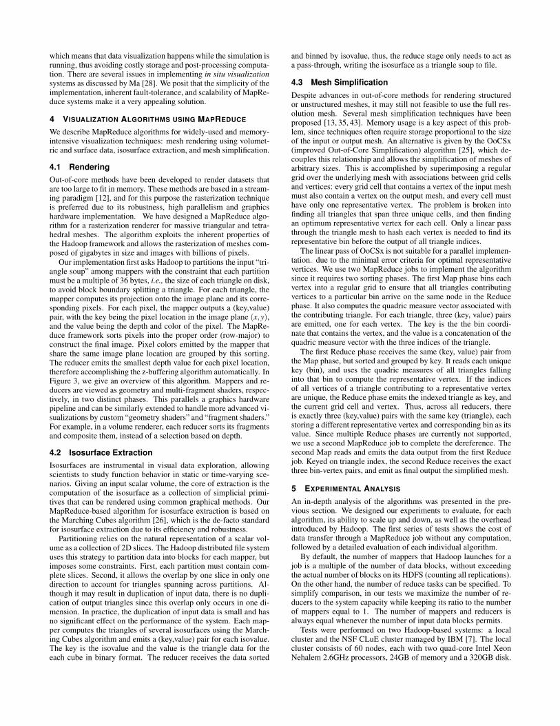
Our implementation first asks Hadoop to partitions the input “tri-angle soup” among mappers with the constraint that each partitionmust be a multiple of 36 bytes, i.e., the size of each triangle on disk,to avoid block boundary splitting a triangle. For each triangle, themapper computes its projection onto the image plane and its corre-sponding pixels. For each pixel, the mapper outputs a (key,value)pair, with the key being the pixel location in the image plane (x,y),and the value being the depth and color of the pixel. The MapRe-duce framework sorts pixels into the proper order (row-major) toconstruct the final image. Pixel colors emitted by the mapper thatshare the same image plane location are grouped by this sorting.The reducer emits the smallest depth value for each pixel location,therefore accomplishing the z-buffering algorithm automatically. InFigure 3, we give an overview of this algorithm. Mappers and re-ducers are viewed as geometry and multi-fragment shaders, respec-tively, in two distinct phases. This parallels a graphics hardwarepipeline and can be similarly extended to handle more advanced vi-sualizations by custom “geometry shaders” and “fragment shaders.”For example, in a volume renderer, each reducer sorts its fragmentsand composite them, instead of a selection based on depth.

4.2 Isosurface ExtractionIsosurfaces are instrumental in visual data exploration, allowingscientists to study function behavior in static or time-varying sce-narios. Giving an input scalar volume, the core of extraction is thecomputation of the isosurface as a collection of simplicial primi-tives that can be rendered using common graphical methods. OurMapReduce-based algorithm for isosurface extraction is based onthe Marching Cubes algorithm [26], which is the de-facto standardfor isosurface extraction due to its efficiency and robustness.

Partitioning relies on the natural representation of a scalar vol-ume as a collection of 2D slices. The Hadoop distributed file systemuses this strategy to partition data into blocks for each mapper, butimposes some constraints. First, each partition must contain com-plete slices. Second, it allows the overlap by one slice in only onedirection to account for triangles spanning across partitions. Al-though it may result in duplication of input data, there is no dupli-cation of output triangles since this overlap only occurs in one di-mension. In practice, the duplication of input data is small and hasno significant effect on the performance of the system. Each map-per computes the triangles of several isosurfaces using the March-ing Cubes algorithm and emits a (key,value) pair for each isovalue.The key is the isovalue and the value is the triangle data for theeach cube in binary format. The reducer receives the data sorted

and binned by isovalue, thus, the reduce stage only needs to act asa pass-through, writing the isosurface as a triangle soup to file.

4.3 Mesh SimplificationDespite advances in out-of-core methods for rendering structuredor unstructured meshes, it may still not feasible to use the full res-olution mesh. Several mesh simplification techniques have beenproposed [13, 35, 43]. Memory usage is a key aspect of this prob-lem, since techniques often require storage proportional to the sizeof the input or output mesh. An alternative is given by the OoCSx(improved Out-of-Core Simplification) algorithm [25], which de-couples this relationship and allows the simplification of meshes ofarbitrary sizes. This is accomplished by superimposing a regulargrid over the underlying mesh with associations between grid cellsand vertices: every grid cell that contains a vertex of the input meshmust also contain a vertex on the output mesh, and every cell musthave only one representative vertex. The problem is broken intofinding all triangles that span three unique cells, and then findingan optimum representative vertex for each cell. Only a linear passthrough the triangle mesh to hash each vertex is needed to find itsrepresentative bin before the output of all triangle indices.

The linear pass of OoCSx is not suitable for a parallel implemen-tation. due to the minimal error criteria for optimal representativevertices. We use two MapReduce jobs to implement the algorithmsince it requires two sorting phases. The first Map phase bins eachvertex into a regular grid to ensure that all triangles contributingvertices to a particular bin arrive on the same node in the Reducephase. It also computes the quadric measure vector associated withthe contributing triangle. For each triangle, three (key, value) pairsare emitted, one for each vertex. The key is the the bin coordi-nate that contains the vertex, and the value is a concatenation of thequadric measure vector with the three indices of the triangle.

The first Reduce phase receives the same (key, value) pair fromthe Map phase, but sorted and grouped by key. It reads each uniquekey (bin), and uses the quadric measures of all triangles fallinginto that bin to compute the representative vertex. If the indicesof all vertices of a triangle contributing to a representative vertexare unique, the Reduce phase emits the indexed triangle as key, andthe current grid cell and vertex. Thus, across all reducers, thereis exactly three (key,value) pairs with the same key (triangle), eachstoring a different representative vertex and corresponding bin as itsvalue. Since multiple Reduce phases are currently not supported,we use a second MapReduce job to complete the dereference. Thesecond Map reads and emits the data output from the first Reducejob. Keyed on triangle index, the second Reduce receives the exactthree bin-vertex pairs, and emit as final output the simplified mesh.

5 EXPERIMENTAL ANALYSIS

An in-depth analysis of the algorithms was presented in the pre-vious section. We designed our experiments to evaluate, for eachalgorithm, its ability to scale up and down, as well as the overheadintroduced by Hadoop. The first series of tests shows the cost ofdata transfer through a MapReduce job without any computation,followed by a detailed evaluation of each individual algorithm.

By default, the number of mappers that Hadoop launches for ajob is a multiple of the number of data blocks, without exceedingthe actual number of blocks on its HDFS (counting all replications).On the other hand, the number of reduce tasks can be specified. Tosimplify comparison, in our tests we maximize the number of re-ducers to the system capacity while keeping its ratio to the numberof mappers equal to 1. The number of mappers and reducers isalways equal whenever the number of input data blocks permits.

Tests were performed on two Hadoop-based systems: a localcluster and the NSF CLuE cluster managed by IBM [7]. The localcluster consists of 60 nodes, each with two quad-core Intel XeonNehalem 2.6GHz processors, 24GB of memory and a 320GB disk.

Map

Input Triangle Soup

Reduce

For each key ( x, y ) : Find minimum z Emit ( x, y, color )

For Each Triangle, T: Rasterize(T):

For each pixel: Emit( x, y, z, color )

Output Image

Figure 3: MapReduce rasterization. The map phase rasterize each triangle and emits rasterized fragments, i.e. the pixel coordinates as key, andits color and depth as value. The reducer composites fragments for each location, e.g. pick the smallest depth one for surface rendering.

The CLuE cluster consists of 410 nodes each with two single-coreIntel Xeon 2.8GHz processors, 4GB of memory and a 400GB disk.While still a valuable resource for research, the CLuE hardwareis outdated if compared to modern clusters, since it was originallybuilt in 2004. Thus, we mostly utilize the performance numbersfrom the CLuE cluster as a way to validate and/or compare withour results on the local cluster. Since the CLuE cluster is a sharedresource among multiple universities, there is currently no way torun experiments in isolation. We made sure to run all of our exper-iments at dead hours to minimize the interference from other jobs.HDFS files were stored in 64MB blocks with 3 replications.

5.1 MapReduce Baseline

To evaluate the cost incurred solely from streaming data throughthe system, several baseline tests were performed. For our scal-ing tests, we have evaluated our algorithms’ performance only forweak-scaling. (i.e., scaling the number of processors with a fixeddata size per processor). This was chosen over strong scaling (i.e.,scaling the number of processors with a fixed total data size) sincethe latter would require changing a data blocksize to adjust the num-ber of mappers appropriately. The Hadoop/HDFS is known fordegraded performance for data with too large or small blocksizesdepending on job complexity [40], therefore strong scaling is cur-rently not a good indicator of performance in Hadoop. The weak-scaling experiments vary data size against task capacity and propor-tionally change the number of mappers and reducers. An algorithmthat has proper weak scaling should maintain a constant runtime. Toavoid biasing results by our optimization schemes, we use the de-fault MapReduce job, with a trivial record reader and writer. Datais stored in binary format and split into 64-byte records, with 16bytes reserved for the key. Map and reduce functions pass the inputdirectly to the output, and are the simplest possible jobs such thatthe performance is disk I/O and network transfer bounded.

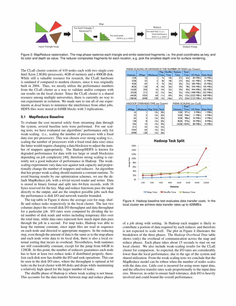
The top table in Figure 4 shows the average cost for map, shuf-fle and reduce tasks respectively in the local cluster. The last twocolumns depict the overall disk I/O throughput and data throughputfor a particular job. I/O rates were computed by dividing the to-tal number of disk reads and writes including temporary files overthe total time, while data rates represent how much input data passthrough the job in a second. For map tasks, Hadoop was able tokeep the runtime constant, since input files are read in sequenceon each node and directed to appropriate mappers. In the reducingstep, even though the amount of data is the same as to the map phaseand each node write data to its local disk, there is also a local ex-ternal sorting that incurs in overhead. Nevertheless, both runtimesare still considerably constant, except for the jump from 64GB to128GB. At this point, the number of reducers guarantees each nodehas to host at least two reduce tasks if distributed properly, there-fore each disk now has double the I/O and seek operations. This canbe seen in the disk I/O rates, where the throughput is optimal at 64tasks on the local cluster with 60 disks and drops while maintaininga relatively high speed for the larger number of tasks.

The shuffle phase of Hadoop is where weak scaling is not linear.This accounts for the data transfer between map and reduce phases

WEAK-SCALING OF DATASIZE VS. THE NUMBER OF TASKS (on Cluster)

Datasize #Maps #ReducesMapTime

ShuffleTime

ReduceTime

Total Time I/O Rate Date Rate

1GB 16 1 7s 18s 27s 63s 84 MB/s 16 MB/s2GB 32 2 8s 18s 27s 66s 161 MB/s 31 MB/s4GB 64 4 9s 24s 30s 75s 283 MB/s 55 MB/s8GB 128 8 10s 26s 29s 78s 545 MB/s 105 MB/s

16GB 256 16 10s 32s 29s 90s 944 MB/s 182 MB/s32GB 512 32 12s 56s 32s 130s 1308 MB/s 252 MB/s64GB 1024 64 11s 69s 30s 153s 2222 MB/s 428 MB/s

128GB 2048 128 13s 146s 57s 320s 2125 MB/s 410 MB/s

HADOOP OVERHEAD TIME (on Cluster) WEAK-SCALING (on CLuE)

#Maps #Reduces Map Only Total DatasizeTotal Time I/O Rate Data Rate

16 1 15s 30s 1GB 971s 5 MB/s 1 MB/s32 2 15s 30s 2GB 946s 11 MB/s 2 MB/s64 4 15s 30s 4GB 986s 22 MB/s 4 MB/s

128 8 15s 30s 8GB 976s 44 MB/s 8 MB/s256 16 15s 30s 16GB 1059s 80 MB/s 15 MB/s512 32 15s 33s

1024 64 15s 35s2048 128 15s 36s

!"#

$!"#

%!"#

&!"#

'!"#

(!!"#

($!"#

(%!"#

(&!"#

()*# $)*# %)*# ')*# (&)*# +$)*# &%)*# ($')*#

!"#$%&#'()*

#'

+%,%-).#'

/%0112'(%-3'425),'

,-.#/012# 34562#/012# 728592#/012#

Figure 4: Hadoop baseline test evaluates data transfer costs. In thelocal cluster we achieve data transfer rates up to 428MB/s

of a job along with sorting. In Hadoop each mapper is likely tocontribute a portion of data required by each reducer, and thereforeis not expected to scale well. The plot in Figure 4 illustrates thebreakdown of the three phases. The Hadoop Overhead Time tableshows (only) the overhead of communication across the map andreduce phases. Each phase takes about 15 seconds to start on ourlocal cluster. We also include weak-scaling results for the CLuEcluster for comparison. As expected, the I/O rates are considerablylower than the local performance, due to the age of the system andshared utilization. From the weak scaling tests we conclude that theMapReduce model can be robust when the number of nodes scaleswith the data size. Little cost is incurred for using more input data,and the effective transfer rates scale proportionally to the input datasize. However, in order to ensure fault tolerance, disk I/O is heavilyinvolved and could bound the overall performance.

(a) Opaque (b) Translucent (c) Color-mapped

WEAK SCALING (RESOLUTION) St. MATTHEW (13 GB) ATLAS (18 GB)

Resolution #M/R CLuE Cluster File #M/R CLuE Cluster Filetime time Written time time Written

1.5 MP 256/256 1min 54s 46s 33MB 273/273 1min 55s 46s 41MB6 MP 256/256 1min 42s 46s 147MB 273/273 2min 11s 46s 104MB

25 MP 256/256 1min 47s 46s 583MB 273/273 2min 12s 46s 412MB100 MP 256/256 1min 40s 46s 2.3GB 273/273 2min 12s 46s 1.6GB400 MP 256/256 2min 04s 46s 10.9GB 273/273 2min 27s 47s 5.5GB1.6 GP 256/256 3min 12s 1min08s 53.14GB 273/273 3min 55s 55s 37.8GB6.4 GP 256/256 9min 50s 2min55s 213GB 273/273 10min 30s 1min58s 151.8GB

WEAK SCALING (RESOLUTION AND REDUCE)St. MATTHEW (13 GB) ATLAS (18 GB)

Resolution CLuE 256M Cluster 480M CLuE 256M Cluster 480M#R time #R time #R time #R time

1.5 MP 4 1min 13s 8 46s 4 1min 18s 8 46s6 MP 8 1min 18s 15 46s 8 1min 19s 15 45s

25 MP 16 1min 18s 30 46s 16 1min 51s 30 46s100 MP 32 2min 04s 60 47s 32 1min 52s 60 47s400 MP 64 2min 04s 120 49s 64 2min 34s 120 46s1.6 GP 128 4min 45s 240 1min06s 128 5min 06s 240 55s6.4 GP 256 9min 50s 480 2min14s 256 10min 30s 480 1min41s

6 MP 25 MP 100 MP 1.6 GP 6.4 GPTime 59s 59s 59s 1m 40s 1m 47s

DAVID (1 Billion Triangles, 30GB)400 MP

1m 1s1.5 MP

59s

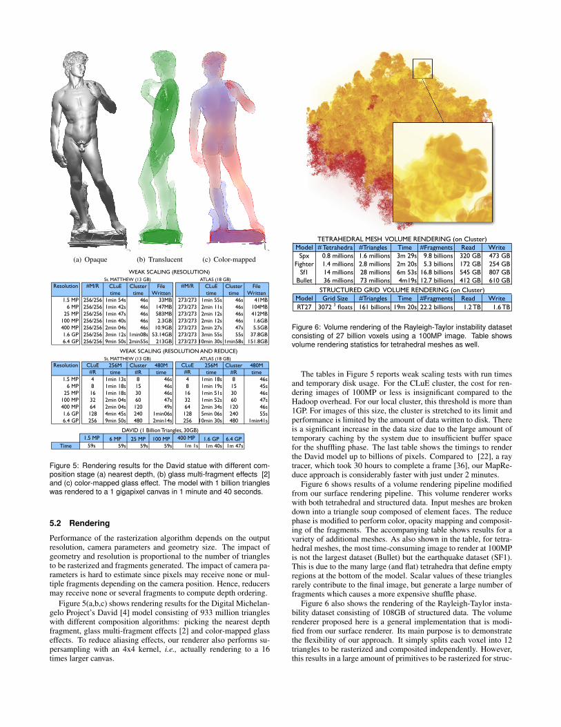
Figure 5: Rendering results for the David statue with different com-position stage (a) nearest depth, (b) glass multi-fragment effects [2]and (c) color-mapped glass effect. The model with 1 billion triangleswas rendered to a 1 gigapixel canvas in 1 minute and 40 seconds.

5.2 Rendering

Performance of the rasterization algorithm depends on the outputresolution, camera parameters and geometry size. The impact ofgeometry and resolution is proportional to the number of trianglesto be rasterized and fragments generated. The impact of camera pa-rameters is hard to estimate since pixels may receive none or mul-tiple fragments depending on the camera position. Hence, reducersmay receive none or several fragments to compute depth ordering.

Figure 5(a,b,c) shows rendering results for the Digital Michelan-gelo Project’s David [4] model consisting of 933 million triangleswith different composition algorithms: picking the nearest depthfragment, glass multi-fragment effects [2] and color-mapped glasseffects. To reduce aliasing effects, our renderer also performs su-persampling with an 4x4 kernel, i.e., actually rendering to a 16times larger canvas.

Model # Tetrahedra #Triangles Time #Fragments Read WriteSpx 0.8 millions 1.6 millions 3m 29s 9.8 billions 320 GB 473 GB

Fighter 1.4 millions 2.8 millions 2m 20s 5.3 billions 172 GB 254 GBSf1 14 millions 28 millions 6m 53s 16.8 billions 545 GB 807 GB

Bullet 36 millions 73 millions 4m19s 12.7 billions 412 GB 610 GB

Model Grid Size #Triangles Time #Fragments Read WriteRT27 3072 3 floats 161 billions 19m 20s 22.2 billions 1.2 TB 1.6 TB

TETRAHEDRAL MESH VOLUME RENDERING (on Cluster)

STRUCTURED GRID VOLUME RENDERING (on Cluster)

Figure 6: Volume rendering of the Rayleigh-Taylor instability datasetconsisting of 27 billion voxels using a 100MP image. Table showsvolume rendering statistics for tetrahedral meshes as well.

The tables in Figure 5 reports weak scaling tests with run timesand temporary disk usage. For the CLuE cluster, the cost for ren-dering images of 100MP or less is insignificant compared to theHadoop overhead. For our local cluster, this threshold is more than1GP. For images of this size, the cluster is stretched to its limit andperformance is limited by the amount of data written to disk. Thereis a significant increase in the data size due to the large amount oftemporary caching by the system due to insufficient buffer spacefor the shuffling phase. The last table shows the timings to renderthe David model up to billions of pixels. Compared to [22], a raytracer, which took 30 hours to complete a frame [36], our MapRe-duce approach is considerably faster with just under 2 minutes.

Figure 6 shows results of a volume rendering pipeline modifiedfrom our surface rendering pipeline. This volume renderer workswith both tetrahedral and structured data. Input meshes are brokendown into a triangle soup composed of element faces. The reducephase is modified to perform color, opacity mapping and composit-ing of the fragments. The accompanying table shows results for avariety of additional meshes. As also shown in the table, for tetra-hedral meshes, the most time-consuming image to render at 100MPis not the largest dataset (Bullet) but the earthquake dataset (SF1).This is due to the many large (and flat) tetrahedra that define emptyregions at the bottom of the model. Scalar values of these trianglesrarely contribute to the final image, but generate a large number offragments which causes a more expensive shuffle phase.

Figure 6 also shows the rendering of the Rayleigh-Taylor insta-bility dataset consisting of 108GB of structured data. The volumerenderer proposed here is a general implementation that is modi-fied from our surface renderer. Its main purpose is to demonstratethe flexibility of our approach. It simply splits each voxel into 12triangles to be rasterized and composited independently. However,this results in a large amount of primitives to be rasterized for struc-

tured grid. Comparing to a structured-grid specific approach [17]that can volume render a similar dataset in 22 seconds using 1728cores, ours is slower with roughly 20 minutes on 256 cores. How-ever, we are in fact rendering 161 billion triangles in this case.

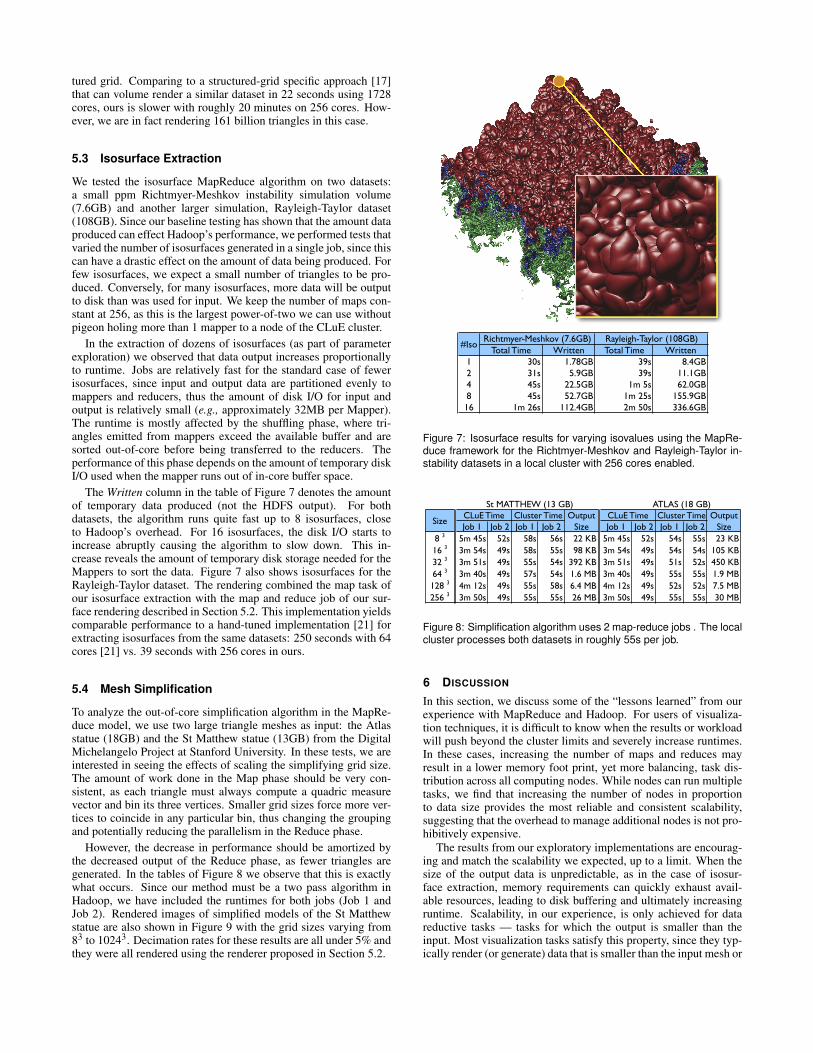
5.3 Isosurface Extraction

We tested the isosurface MapReduce algorithm on two datasets:a small ppm Richtmyer-Meshkov instability simulation volume(7.6GB) and another larger simulation, Rayleigh-Taylor dataset(108GB). Since our baseline testing has shown that the amount dataproduced can effect Hadoop’s performance, we performed tests thatvaried the number of isosurfaces generated in a single job, since thiscan have a drastic effect on the amount of data being produced. Forfew isosurfaces, we expect a small number of triangles to be pro-duced. Conversely, for many isosurfaces, more data will be outputto disk than was used for input. We keep the number of maps con-stant at 256, as this is the largest power-of-two we can use withoutpigeon holing more than 1 mapper to a node of the CLuE cluster.

In the extraction of dozens of isosurfaces (as part of parameterexploration) we observed that data output increases proportionallyto runtime. Jobs are relatively fast for the standard case of fewerisosurfaces, since input and output data are partitioned evenly tomappers and reducers, thus the amount of disk I/O for input andoutput is relatively small (e.g., approximately 32MB per Mapper).The runtime is mostly affected by the shuffling phase, where tri-angles emitted from mappers exceed the available buffer and aresorted out-of-core before being transferred to the reducers. Theperformance of this phase depends on the amount of temporary diskI/O used when the mapper runs out of in-core buffer space.

The Written column in the table of Figure 7 denotes the amountof temporary data produced (not the HDFS output). For bothdatasets, the algorithm runs quite fast up to 8 isosurfaces, closeto Hadoop’s overhead. For 16 isosurfaces, the disk I/O starts toincrease abruptly causing the algorithm to slow down. This in-crease reveals the amount of temporary disk storage needed for theMappers to sort the data. Figure 7 also shows isosurfaces for theRayleigh-Taylor dataset. The rendering combined the map task ofour isosurface extraction with the map and reduce job of our sur-face rendering described in Section 5.2. This implementation yieldscomparable performance to a hand-tuned implementation [21] forextracting isosurfaces from the same datasets: 250 seconds with 64cores [21] vs. 39 seconds with 256 cores in ours.

5.4 Mesh Simplification

To analyze the out-of-core simplification algorithm in the MapRe-duce model, we use two large triangle meshes as input: the Atlasstatue (18GB) and the St Matthew statue (13GB) from the DigitalMichelangelo Project at Stanford University. In these tests, we areinterested in seeing the effects of scaling the simplifying grid size.The amount of work done in the Map phase should be very con-sistent, as each triangle must always compute a quadric measurevector and bin its three vertices. Smaller grid sizes force more ver-tices to coincide in any particular bin, thus changing the groupingand potentially reducing the parallelism in the Reduce phase.

However, the decrease in performance should be amortized bythe decreased output of the Reduce phase, as fewer triangles aregenerated. In the tables of Figure 8 we observe that this is exactlywhat occurs. Since our method must be a two pass algorithm inHadoop, we have included the runtimes for both jobs (Job 1 andJob 2). Rendered images of simplified models of the St Matthewstatue are also shown in Figure 9 with the grid sizes varying from83 to 10243. Decimation rates for these results are all under 5% andthey were all rendered using the renderer proposed in Section 5.2.

Total Time Written Total Time Written1 30s 1.78GB 39s 8.4GB2 31s 5.9GB 39s 11.1GB4 45s 22.5GB 1m 5s 62.0GB8 45s 52.7GB 1m 25s 155.9GB16 1m 26s 112.4GB 2m 50s 336.6GB

Richtmyer-Meshkov (7.6GB) Rayleigh-Taylor (108GB)#Iso

Figure 7: Isosurface results for varying isovalues using the MapRe-duce framework for the Richtmyer-Meshkov and Rayleigh-Taylor in-stability datasets in a local cluster with 256 cores enabled.

Job 1 Job 2 Job 1 Job 2 Job 1 Job 2 Job 1 Job 28 3 5m 45s 52s 58s 56s 22 KB 5m 45s 52s 54s 55s 23 KB16 3 3m 54s 49s 58s 55s 98 KB 3m 54s 49s 54s 54s 105 KB32 3 3m 51s 49s 55s 54s 392 KB 3m 51s 49s 51s 52s 450 KB64 3 3m 40s 49s 57s 54s 1.6 MB 3m 40s 49s 55s 55s 1.9 MB128 3 4m 12s 49s 55s 58s 6.4 MB 4m 12s 49s 52s 52s 7.5 MB256 3 3m 50s 49s 55s 55s 26 MB 3m 50s 49s 55s 55s 30 MB

CLuE Time Cluster Time ATLAS (18 GB)

CLuE Time Cluster TimeSize

OutputSize

OutputSize

St MATTHEW (13 GB)

Figure 8: Simplification algorithm uses 2 map-reduce jobs . The localcluster processes both datasets in roughly 55s per job.

6 DISCUSSION

In this section, we discuss some of the “lessons learned” from ourexperience with MapReduce and Hadoop. For users of visualiza-tion techniques, it is difficult to know when the results or workloadwill push beyond the cluster limits and severely increase runtimes.In these cases, increasing the number of maps and reduces mayresult in a lower memory foot print, yet more balancing, task dis-tribution across all computing nodes. While nodes can run multipletasks, we find that increasing the number of nodes in proportionto data size provides the most reliable and consistent scalability,suggesting that the overhead to manage additional nodes is not pro-hibitively expensive.

The results from our exploratory implementations are encourag-ing and match the scalability we expected, up to a limit. When thesize of the output data is unpredictable, as in the case of isosur-face extraction, memory requirements can quickly exhaust avail-able resources, leading to disk buffering and ultimately increasingruntime. Scalability, in our experience, is only achieved for datareductive tasks — tasks for which the output is smaller than theinput. Most visualization tasks satisfy this property, since they typ-ically render (or generate) data that is smaller than the input mesh or

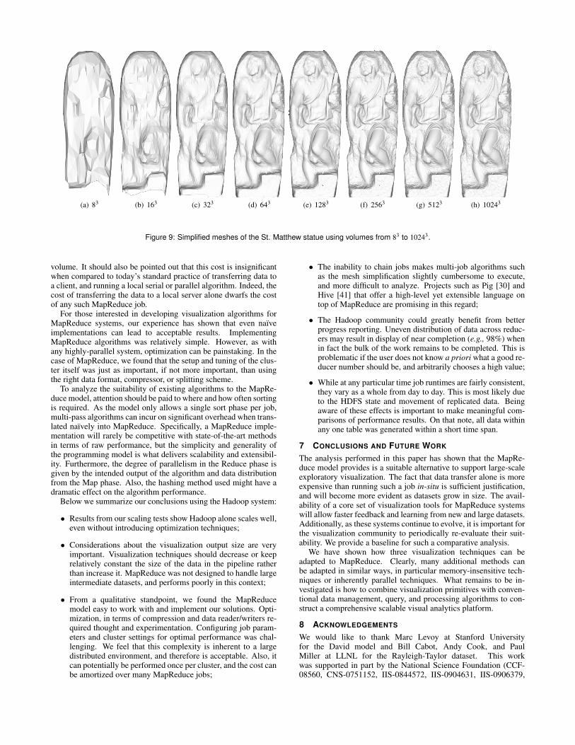
(a) 83 (b) 163 (c) 323 (d) 643 (e) 1283 (f) 2563 (g) 5123 (h) 10243

Figure 9: Simplified meshes of the St. Matthew statue using volumes from 83 to 10243.

volume. It should also be pointed out that this cost is insignificantwhen compared to today’s standard practice of transferring data toa client, and running a local serial or parallel algorithm. Indeed, thecost of transferring the data to a local server alone dwarfs the costof any such MapReduce job.

For those interested in developing visualization algorithms forMapReduce systems, our experience has shown that even naıveimplementations can lead to acceptable results. ImplementingMapReduce algorithms was relatively simple. However, as withany highly-parallel system, optimization can be painstaking. In thecase of MapReduce, we found that the setup and tuning of the clus-ter itself was just as important, if not more important, than usingthe right data format, compressor, or splitting scheme.

To analyze the suitability of existing algorithms to the MapRe-duce model, attention should be paid to where and how often sortingis required. As the model only allows a single sort phase per job,multi-pass algorithms can incur on significant overhead when trans-lated naıvely into MapReduce. Specifically, a MapReduce imple-mentation will rarely be competitive with state-of-the-art methodsin terms of raw performance, but the simplicity and generality ofthe programming model is what delivers scalability and extensibil-ity. Furthermore, the degree of parallelism in the Reduce phase isgiven by the intended output of the algorithm and data distributionfrom the Map phase. Also, the hashing method used might have adramatic effect on the algorithm performance.

Below we summarize our conclusions using the Hadoop system:

• Results from our scaling tests show Hadoop alone scales well,even without introducing optimization techniques;

• Considerations about the visualization output size are veryimportant. Visualization techniques should decrease or keeprelatively constant the size of the data in the pipeline ratherthan increase it. MapReduce was not designed to handle largeintermediate datasets, and performs poorly in this context;

• From a qualitative standpoint, we found the MapReducemodel easy to work with and implement our solutions. Opti-mization, in terms of compression and data reader/writers re-quired thought and experimentation. Configuring job param-eters and cluster settings for optimal performance was chal-lenging. We feel that this complexity is inherent to a largedistributed environment, and therefore is acceptable. Also, itcan potentially be performed once per cluster, and the cost canbe amortized over many MapReduce jobs;

• The inability to chain jobs makes multi-job algorithms suchas the mesh simplification slightly cumbersome to execute,and more difficult to analyze. Projects such as Pig [30] andHive [41] that offer a high-level yet extensible language ontop of MapReduce are promising in this regard;

• The Hadoop community could greatly benefit from betterprogress reporting. Uneven distribution of data across reduc-ers may result in display of near completion (e.g., 98%) whenin fact the bulk of the work remains to be completed. This isproblematic if the user does not know a priori what a good re-ducer number should be, and arbitrarily chooses a high value;

• While at any particular time job runtimes are fairly consistent,they vary as a whole from day to day. This is most likely dueto the HDFS state and movement of replicated data. Beingaware of these effects is important to make meaningful com-parisons of performance results. On that note, all data withinany one table was generated within a short time span.

7 CONCLUSIONS AND FUTURE WORK

The analysis performed in this paper has shown that the MapRe-duce model provides is a suitable alternative to support large-scaleexploratory visualization. The fact that data transfer alone is moreexpensive than running such a job in-situ is sufficient justification,and will become more evident as datasets grow in size. The avail-ability of a core set of visualization tools for MapReduce systemswill allow faster feedback and learning from new and large datasets.Additionally, as these systems continue to evolve, it is important forthe visualization community to periodically re-evaluate their suit-ability. We provide a baseline for such a comparative analysis.

We have shown how three visualization techniques can beadapted to MapReduce. Clearly, many additional methods canbe adapted in similar ways, in particular memory-insensitive tech-niques or inherently parallel techniques. What remains to be in-vestigated is how to combine visualization primitives with conven-tional data management, query, and processing algorithms to con-struct a comprehensive scalable visual analytics platform.

8 ACKNOWLEDGEMENTS

We would like to thank Marc Levoy at Stanford Universityfor the David model and Bill Cabot, Andy Cook, and PaulMiller at LLNL for the Rayleigh-Taylor dataset. This workwas supported in part by the National Science Foundation (CCF-08560, CNS-0751152, IIS-0844572, IIS-0904631, IIS-0906379,

and CCF-0702817), the Department of Energy, CNPq (processes200498/2010-0, 569239/2008-7, and 491034/2008-3), IBM Fac-ulty Awards and NVIDIA Fellowships. This work was also per-formed under the auspices of the U.S. Department of Energy by theUniversity of Utah under contract DE-SC0001922 and DE-FC02-06ER25781 and by Lawrence Livermore National Laboratory un-der contract DE-AC52-07NA27344, LLNL-JRNL-453051.

REFERENCES

[1] Amazon web services - elastic mapreduce. http://aws.amazon.

com/elasticmapreduce/.[2] L. Bavoil, S. P. Callahan, A. Lefohn, J. a. L. D. Comba, and C. T. Silva.

Multi-fragment effects on the gpu using the k-buffer. In Proceedingsof the 2007 symposium on Interactive 3D graphics and games, I3D’07, pages 97–104, New York, NY, USA, 2007. ACM.

[3] D. Borthakur. The Hadoop distributed file system: Architectureand design. http://lucene.apache.org/hadoop/hdfs_design.pdf, 2007.

[4] B. Brown and S. Rusinkiewicz. Global non-rigid alignment of 3-Dscans. ACM Transactions on Graphics (Proc. SIGGRAPH), 26(3),Aug. 2007.

[5] R. Chaiken, B. Jenkins, P.-A. Larson, B. Ramsey, D. Shakib,S. Weaver, and J. Zhou. Scope: easy and efficient parallel process-ing of massive data sets. In Proc. of the 34th Int. Conf. on Very LargeDataBases (VLDB), pages 1265–1276, 2008.

[6] F. Chang, J. Dean, S. Ghemawat, W. C. Hsieh, D. A. Wallach, M. Bur-rows, T. Chandra, A. Fikes, and R. E. Gruber. Bigtable: a distributedstorage system for structured data. In Proc. of the 7th USENIX Symp.on Operating Systems Design & Implementation (OSDI), 2006.

[7] Nsf cluster exploratory (nsf08560). http://www.nsf.gov/pubs/

2008/nsf08560/nsf08560.htm.[8] J. Dean and S. Ghemawat. MapReduce: simplified data processing

on large clusters. In Proc. of the 6th USENIX Symp. on OperatingSystems Design & Implementation (OSDI), 2004.

[9] J. Dean and S. Ghemawat. MapReduce: simplified data processing onlarge clusters. CACM, 51(1):107–113, 2008.

[10] G. DeCandia, D. Hastorun, M. Jampani, G. Kakulapati, A. Laksh-man, A. Pilchin, S. Sivasubramanian, P. Vosshall, and W. Vogels. Dy-namo: Amazon’s highly available key-value store. In Proc. of the 21stACM Symp. on Operating Systems Principles (SOSP), pages 205–220,2007.

[11] D. J. DeWitt, E. Paulson, E. Robinson, J. Naughton, J. Royalty,S. Shankar, and A. Krioukov. Clustera: an integrated computationand data management system. In Proc. of the 34th Int. Conf. on VeryLarge DataBases (VLDB), pages 28–41, 2008.

[12] R. Farias and C. T. Silva. Out-of-core rendering of large, unstructuredgrids. IEEE Comput. Graph. Appl., 21(4):42–50, 2001.

[13] M. Garland and P. S. Heckbert. Surface simplification using quadricerror metrics. In SIGGRAPH ’97: Proceedings of the 24th annualconference on Computer graphics and interactive techniques, pages209–216, New York, NY, USA, 1997. ACM Press/Addison-WesleyPublishing Co.

[14] Hadoop. http://hadoop.apache.org/.[15] G. Heber and J. Gray. Supporting finite element analysis with a rela-

tional database backend; part 1: There is life beyond files. Technicalreport, Microsoft MSR-TR-2005-49, April 2005.

[16] Hive. http://hadoop.apache.org/hive/. Accessed March 7,2010.

[17] M. Howison, W. Bethel, and H. Childs. Mpi-hybrid parallelism forvolume rendering on large, multi-core systems. In EG Symposium onParallel Graphics and Visualization (EGPGV’10), 2010.

[18] IBM Systems and Technology Group. IBM Deep Computing. Tech-nical report, IBM, 2005.

[19] Incorporated Research Institutions for Seismology (IRIS). http://

www.iris.edu/.[20] M. Isard, M. Budiu, Y. Yu, A. Birrell, and D. Fetterly. Dryad: Dis-

tributed data-parallel programs from sequential building blocks. InProc. of the European Conference on Computer Systems (EuroSys),pages 59–72, 2007.

[21] M. Isenburg, P. Lindstrom, and H. Childs. Parallel and streaming gen-eration of ghost data for structured grids. Computer Graphics andApplications, IEEE, 30(3):32–44, 2010.

[22] T. Ize, C. Brownlee, and C. Hansen. Real-time ray tracer for visu-alizing massive models on a cluster. In EG Symposium on ParallelGraphics and Visualization (EGPGV’11), 2011.

[23] Kosmix Corp. Kosmos distributed file system (kfs). http://

kosmosfs.sourceforge.net, 2007.[24] Lawrence Livermore National Laboratory. VisIt: Visualize It in Par-

allel Visualization Application. https://wci.llnl.gov/codes/

visit [29 March 2008].[25] P. Lindstrom and C. T. Silva. A memory insensitive technique for

large model simplification. In VIS ’01: Proceedings of the conferenceon Visualization ’01, pages 121–126, Washington, DC, USA, 2001.IEEE Computer Society.

[26] W. Lorensen and H. Cline. Marching cubes: A high resolution 3Dsurface construction algorithm. Computer Graphics, 21(4):163–169,1987.

[27] Large Synoptic Survey Telescope. http://www.lsst.org/.[28] K.-L. Ma. In situ visualization at extreme scale: Challenges and op-

portunities. Computer Graphics and Applications, IEEE, 29(6):14 –19, nov.-dec. 2009.

[29] Azure Services Platform - SQL Data Services. http://www.

microsoft.com/azure/data.mspx.[30] C. Olston, B. Reed, U. Srivastava, R. Kumar, and A. Tomkins. Pig

latin: a not-so-foreign language for data processing. In SIGMOD’08:Proc. of the ACM SIGMOD Int. Conf. on Management of Data, pages1099–1110, 2008.

[31] Paraview. http://www.paraview.org [29 March 2008].[32] B. Paul, S. Ahern, E. W. Bethel, E. Brugger, R. Cook, J. Daniel,

K. Lewis, J. Owen, and D. Southard. Chromium Renderserver: Scal-able and Open Remote Rendering Infrastructure. IEEE Transac-tions on Visualization and Computer Graphics, 14(3), May/June 2008.LBNL-63693.

[33] A. Pavlo, E. Paulson, A. Rasin, D. J. Abadi, D. J. DeWitt, S. R. Mad-den, and M. Stonebraker. A comparison of approaches to large scaledata analysis. In SIGMOD, Providence, Rhode Island, USA, 2009.

[34] T. Richardson, Q. Stafford-Fraser, K. R. Wood, and A. Hopper. Virtualnetwork computing. IEEE Internet Computing, 2(1):33–38, 1998.

[35] W. J. Schroeder, J. A. Zarge, and W. E. Lorensen. Decimation oftriangle meshes. In SIGGRAPH ’92: Proceedings of the 19th annualconference on Computer graphics and interactive techniques, pages65–70, New York, NY, USA, 1992. ACM.

[36] U. o. U. SCI Institute. One billion polygons to billions of pixels.http://www.sci.utah.edu/news/60/431-visus.html.

[37] Silicon Graphics Inc. OpenGL vizserver. http://www.sgi.com/

products/software/vizserver.[38] Sloan Digital Sky Survey. http://cas.sdss.org.[39] S. Stegmaier, M. Magallon, and T. Ertl. A generic solution for

hardware-accelerated remote visualization. In VISSYM ’02: Proceed-ings of the symposium on Data Visualisation 2002, pages 87–ff, Aire-la-Ville, Switzerland, Switzerland, 2002. Eurographics Association.

[40] I. Technologies. Hadoop performance tuning - white paper.[41] A. Thusoo, J. S. Sarma, N. Jain, Z. Shao, P. Chakka, S. Anthony,

H. Liu, P. Wyckoff, and R. Murthy. Hive - a warehousing solutionover a map-reduce framework. PVLDB, 2(2):1626–1629, 2009.

[42] Yahoo! Reasearch. PNUTS - Platform for Nimble Universal TableStorage. http://research.yahoo.com/node/212.

[43] J. Yan, P. Shi, and D. Zhang. Mesh simplification with hierarchicalshape analysis and iterative edge contraction. IEEE Transactions onVisualization and Computer Graphics, 10(2):142–151, 2004.

[44] H. Yang, A. Dasdan, R.-L. Hsiao, and D. S. Parker. Map-reduce-merge: simplified relational data processing on large clusters. In SIG-MOD’07: Proc. of the ACM SIGMOD Int. Conf. on Management ofData, pages 1029–1040, 2007.

[45] Y. Yu, M. Isard, D. Fetterly, M. Budiu, U. Erlingsson, P. K. Gunda,and J. Currey. DryadLINQ: A system for general-purpose distributeddata-parallel computing using a high-level language. In Proc. of the8th USENIX Symp. on Operating Systems Design & Implementation(OSDI), 2008.