parallel monte carlo simulations of light propagation …bmlaser.physics.ecu.edu/literature/2000_wu...
TRANSCRIPT

PARALLEL MONTE CARLO SIMULATIONS OF LIGHT
PROPAGATION IN TURBID MEDIA
A Thesis
Presented to
the Faculty of the Department of Physics
East Carolina University
In Partial Fulfillment
of the Requirements for the Degree
Master of Science in Applied Physics
by
Di Wu
July 2000
Abstract
Di Wu PARALLEL MONTE CARLO SIMULATIONS OF LIGHT PROPAGATION IN TURBID MEDIA. (Under the direction of Dr. Jun Qing Lu) Department of Physics, July 2000.
We have carried out investigation on light propagating in turbid media using parallel
Monte Carlo method. Through this project, we built a 32-node UNIX cluster to provide a
powerful parallel computing environment and successfully converted sequential Monte
Carlo simulation program to parallel program using both MPI and PVM message passing
parallel computing interface software packages. In addition, random number generator
algorithms are carefully studied and a portable parallel random number generator has
been developed to meet our parallel Monte Carlo simulation needs. These developments
are then used to carry out large-scale numerical simulations of a converging light beam
propagating through a biological tissue slab. Our results on the dependence of the photon
density at the focal point on the attenuation coefficient µt show that the peak observed
there is formed by the unattenuated photons. The results of statistical distributions of the
reflected and transmitted photons show that the reflected photons experience much less
scattering than those of transmitted. The dependence of the reflectivity, transmittance,
and absorption of the incident light on the parameters µt and g has also been studied.

PARALLEL MONTE CARLO SIMULATIONS OF LIGHT
PROPAGATION IN TURBID MEDIA
by
Di Wu
APPROVED BY: DIRECTOR OF THESIS__________________________________________________
JUN Q. LU, Ph.D.
COMMITTEE MEMBER_______________________________________________ XIN-HUA HU, Ph.D.
COMMITTEE MEMBER__________________________________________________ JAMES M. JOYCE, Ph.D.
COMMITTEE MEMBER__________________________________________________ MOHAMMAD SALEHPOUR, Ph.D.
CHAIR OF THE DEPARTMENT OF PHYSICS________________________________ CHARLES E. BLAND, Ph.D.
DEAN OF THE GRADUATE SCHOOL_______________________________________ THOMAS L. FELDBUSH, Ph.D.

Acknowledgements
First of all, I would like to thank the physics department for their support and
encouragement throughout my study and research of this work.
I will give my most appreciations to my advisor Dr. Jun Qing Lu for her
immeasurable help and encouragement since I started working on this project. She is
always kind and patient to me despite my many questions and slowness. Without her, I
would not have pursued a master’s degree. I am also very grateful to Dr. Xin-Hua Hu, for
teaching me plenty of physics and guiding me to become a real graduate student and
researcher. Also, I would like to thank Mr. Suisheng Zhao for giving us precious advices
on our network setup and parallel programming.
My acknowledgement is extended to Dr. Joyce and Dr. Salehpour for their
serving on my thesis committee, reviewing this manuscript, and for making sure I met all
the graduation requirements set by the department and the university.
I would also thank my friends Yong Du, Qiqin Fang and Ke Dong in the physics
department for their support and help in both research and personality. Many thanks to
Scott Brock for testing our random number generator and helping us improve our
network.
Finally, I owe my gratitude to my parents and my uncle and aunt for their
continuing support of my further education and my girlfriend Bei Ma, for her company,
encouragement and caring throughout this project and thesis.
Some numerical simulations were performed on the Cray T3E super computer
through a grant from the North Carolina Supercomputing Center. Research assistantship

has been provided through the grants from National Science Foundation (#PHY-
9973787) and National Institute of Health (R15GM/OD55940-01).
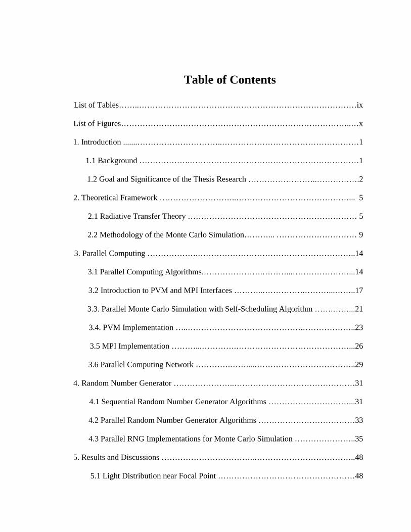
Table of Contents
List of Tables……..………………………………………………………………………ix
List of Figures…………………………………………………………………………..…x
1. Introduction .......…………………………..……………………………………………1
1.1 Background ……………….………………………………………………………1
1.2 Goal and Significance of the Thesis Research ……………………..…………….2
2. Theoretical Framework ………………………..……………………………………... 5
2.1 Radiative Transfer Theory ……………………………………………………… 5
2.2 Methodology of the Monte Carlo Simulation………... ………………………… 9
3. Parallel Computing ……………….…………………………………………………..14
3.1 Parallel Computing Algorithms.………………….………...…………………...14
3.2 Introduction to PVM and MPI Interfaces ………..…………….………...……..17
3.3. Parallel Monte Carlo Simulation with Self-Scheduling Algorithm …….……...21
3.4. PVM Implementation …..…………………………………….………………..23
3.5 MPI Implementation ………...………….……………………………………...26
3.6 Parallel Computing Network ………….……....………………………………..29
4. Random Number Generator …………………..………………………………………31
4.1 Sequential Random Number Generator Algorithms …………………………...31
4.2 Parallel Random Number Generator Algorithms ………………………………33
4.3 Parallel RNG Implementations for Monte Carlo Simulation …………………..35
5. Results and Discussions ……………………………..………………………………..48
5.1 Light Distribution near Focal Point ……………………………………………48

viii
5.2 Unattenuated Photon Density at Focal Point…………………….……………..55
5.3 Transmission, Reflectivity and Absorption ……………………………………57
5.4 Scattering Statistics of the Reflected and Transmitted Photons………………..61
6. Summary……………………..………………………………………..………………64
References ……………………………………………………………………………...66
Appendix A: System Installation and Administration For the PC-Cluster……….……..70
Appendix B: PVM and MPI Setup ……………………………………………………...88
Appendix C: SPRNG ……………………………………………………………………93
Appendix D: Source Codes…………………………………………………………..…100

List of Tables
4.1 Statistic testing results for RAN4 and RAN2……………………………………..…44
List of Figures
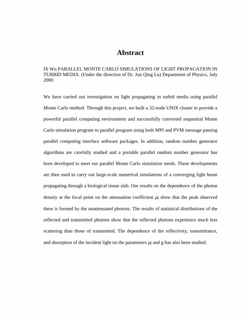
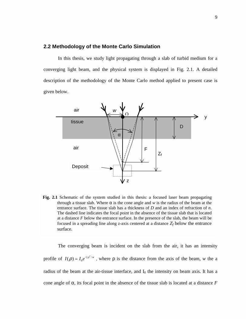
1: Schematic of the system studied in this thesis: a focused laser beam propagating through a tissue slab. Where α is the cone angle and w is the radius of the beam at the entrance surface. The tissue slab has a thickness of D and an index of refraction of n. The dashed line indicates the focal point in the absence of the tissue slab that is located at a distance F below the entrance surface. In the presence of the slab, the beam will be focused in a spreading line along z-axis
centered at a distance Zf below the entrance surface………………….………………..9
2: In our parallel computing, photons in the incident beam are divided into groups (tasks). Different computer processes different task independently and concurrently. All tasks, which running on slaves, are controlled and coordinated by master. When finished, result of each task is reported back to master. Master thus collects all the results from these tasks and finally combines them to generate the final result. The combined result should be equivalent to the
original sequential result………………………………….………………………..….22
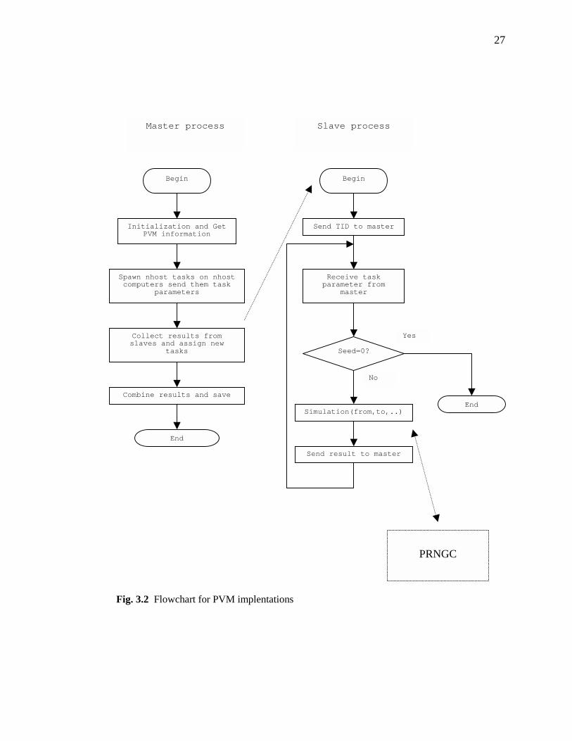
3: Flowchart for PVM implementations……………………………….…………...……27
4: Flowchart for MPI implementations……………………………………………....…..28
5: Flowchart for PRNGC…………………………………………………….………......29
6: The architecture of our workstation cluster and server. The server shares its resources with workstations via NFS…………………………...……………………..30
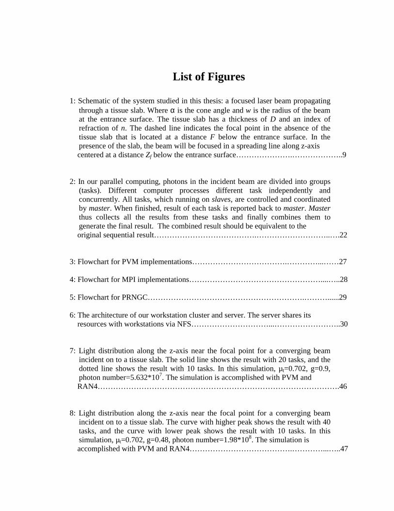
7: Light distribution along the z-axis near the focal point for a converging beam incident on to a tissue slab. The solid line shows the result with 20 tasks, and the dotted line shows the result with 10 tasks. In this simulation, µt=0.702, g=0.9, photon number=5.632*107. The simulation is accomplished with PVM and
RAN4………………………………………………………………………………….46
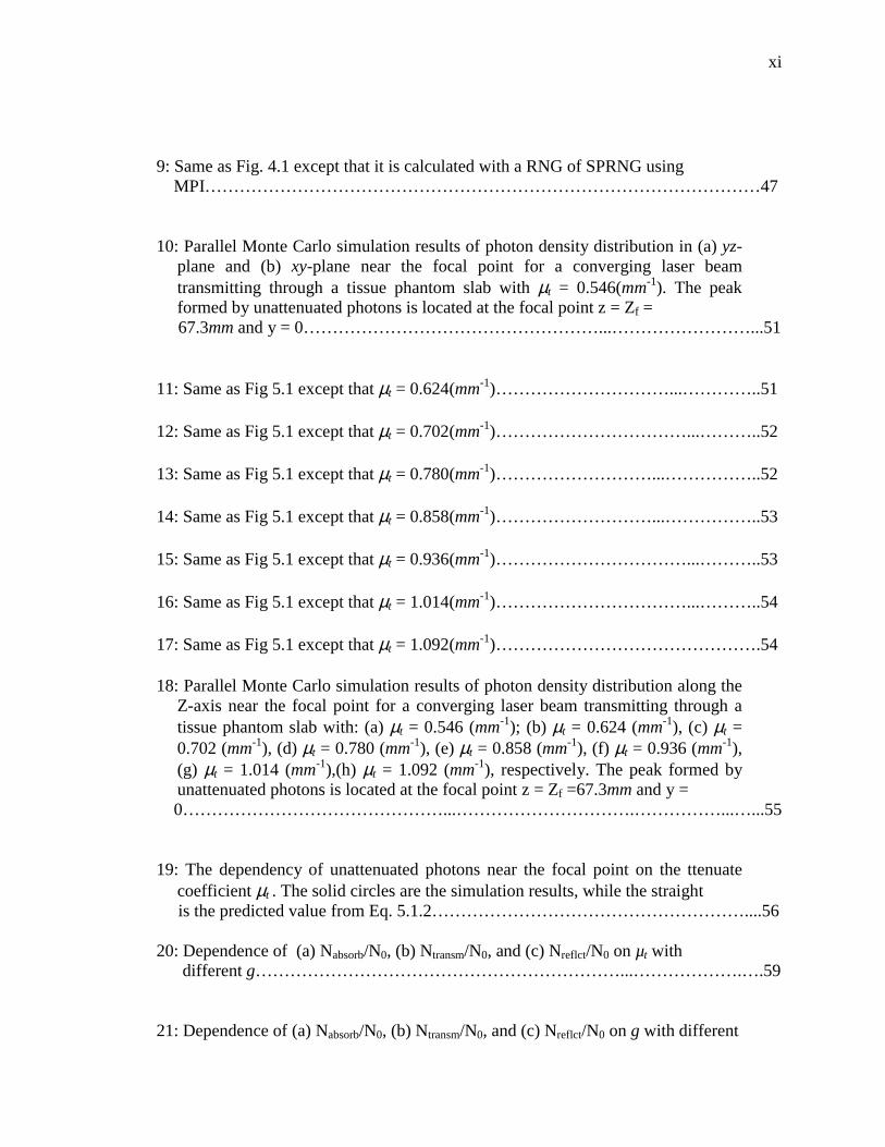
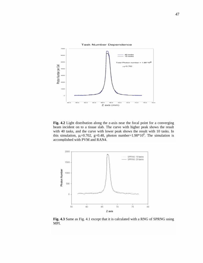
8: Light distribution along the z-axis near the focal point for a converging beam incident on to a tissue slab. The curve with higher peak shows the result with 40 tasks, and the curve with lower peak shows the result with 10 tasks. In this simulation, µt=0.702, g=0.48, photon number=1.98*108. The simulation is
accomplished with PVM and RAN4………………………………….…………...…..47
xi
9: Same as Fig. 4.1 except that it is calculated with a RNG of SPRNG using MPI……………………………………………………………………………………47
10: Parallel Monte Carlo simulation results of photon density distribution in (a) yz-plane and (b) xy-plane near the focal point for a converging laser beam transmitting through a tissue phantom slab with µt = 0.546(mm-1). The peak formed by unattenuated photons is located at the focal point z = Zf =
67.3mm and y = 0……………………………………………...……………………...51
11: Same as Fig 5.1 except that µt = 0.624(mm-1)…………………………...…………..51
12: Same as Fig 5.1 except that µt = 0.702(mm-1)……………………………...………..52
13: Same as Fig 5.1 except that µt = 0.780(mm-1)………………………...……………..52
14: Same as Fig 5.1 except that µt = 0.858(mm-1)………………………...……………..53
15: Same as Fig 5.1 except that µt = 0.936(mm-1)……………………………...………..53
16: Same as Fig 5.1 except that µt = 1.014(mm-1)……………………………...………..54
17: Same as Fig 5.1 except that µt = 1.092(mm-1)……………………………………….54
18: Parallel Monte Carlo simulation results of photon density distribution along the Z-axis near the focal point for a converging laser beam transmitting through a tissue phantom slab with: (a) µt = 0.546 (mm-1); (b) µt = 0.624 (mm-1), (c) µt = 0.702 (mm-1), (d) µt = 0.780 (mm-1), (e) µt = 0.858 (mm-1), (f) µt = 0.936 (mm-1), (g) µt = 1.014 (mm-1),(h) µt = 1.092 (mm-1), respectively. The peak formed by unattenuated photons is located at the focal point z = Zf =67.3mm and y =
0………………………………………...………………………….……………...…...55
19: The dependency of unattenuated photons near the focal point on the ttenuate coefficient µt . The solid circles are the simulation results, while the straight
is the predicted value from Eq. 5.1.2………………………………………………....56 20: Dependence of (a) Nabsorb/N0, (b) Ntransm/N0, and (c) Nreflct/N0 on µt with different g………………………………………………………...……………….….59
21: Dependence of (a) Nabsorb/N0, (b) Ntransm/N0, and (c) Nreflct/N0 on g with different
xii
µt………………………………………………………………………………...……60
22: Results for a given number of scatterings the observed number of photons in the reflected light at a given distance from the axis of the incident beam in the
entrance plane……………………...………………………………………………....62
23: Results for a given number of scatterings the observed number of photons in the transmitted light at a given distance from the axis of the incident beam in the
focal plane……………………..…………………………………………...…………62
24: Same as Fig. 5.13 except that g=0.48…………………………………………….….63
25: Same as Fig. 5.14 except that g=0.48………………………………….…………….63

1. Introduction 1.1 Background
Light scattering in the turbid media has been studied extensively in the past
[Ishimara, 1978]. Many attempts have been made to provide reasonably accurate, and yet
feasible, models of light propagation in turbid media. However, the existing theoretical
models are still not satisfactory for explaining the experimental data in many important
applications related to the light propagation in highly scattering turbid media such as
biological materials. Understanding the interaction between light and biological materials
is critical in the development of new optical methods for biomedical imaging
applications. For this purpose, it is essential to develop efficient modeling tools in the
investigation of interaction between laser radiation and turbid media.
In a turbid medium, light is scattered and absorbed due to the inhomogeneities
and absorption characteristics of the medium. When the medium becomes highly
scattering, multiple scattering effects become dominant, and one widely used approach to
solve this type of problem is the radiative transfer theory [Chandrasekhar, 1960] - which
concerns only the energy transportation. Within the framework of the radiative transfer
theory, light propagation in a turbid medium is treated as a large number of photons,
which have no phase and polarization characteristics, which undergo random scattering
and absorption processes. However, the radiative transfer equation cannot be solved
analytically without approximations except for a few cases with simple boundary
conditions. Among these are the first-order solution [Ishimaru, 1978], the discrete
ordinates method [Ishimaru, 1978], the Kubelka-Munk two-flux and four-flux theory

2
[Wan, 1981], and the diffusion theory [Johnson, 1970]. These methods all have their
limits.
Light propagation in turbid medium can be simulated statistically by Monte Carlo
methods [Wilson, 1983]. Using a simple model of random walk, a Monte Carlo method
can be applied to solve radiative transfer problems accurately with virtually any boundary
conditions. Among many Monte Carlo methods used to simulation light–tissue
interaction, a recently developed Monte Carlo method using a “time slicing” algorithm
can be used to directly calculate light distribution with inhomogeneous boundary
conditions [Song, 1999]. Two examples of the inhomogeneous boundary conditions are:
a converging laser beam incident on a tissue phantom with a plane surface in which the
incident angle varies with the photon location; a tissue phantom with rough interfaces in
which the incident angle varies with fluctuating direction of the surface normal even for a
collimated beam.
1.2 Goal and Significance of the Thesis Research
Monte Carlo method offers a flexible yet rigorous approach toward modeling of
photon transportation inside highly scattering media. This method, however, relies
heavily on computer tracking of the propagation paths of individual photons in the
medium. It is very computationally intensive due to the statistical nature of the large
number of photons needed to achieve precision and resolution. On the other hand, the
uncorrelated-photon nature in the Radiative Transfer Theory makes this problem a unique
candidate for parallel processing.

3
The goal of this thesis is to implement parallel computing techniques in the Monte
Carlo simulation of light propagating in turbid media and to use the parallel Monte Carlo
method to investigate various phenomena associated with light propagation in a slab of
turbid medium for a converging incident beam. Due to the inhomogeneous boundary
condition in the studied system, the “time-slicing” Monte Carlo method discussed earlier
will be used to carry out the simulations.
By implementing parallel computation techniques in the Monte Carlo simulation,
we can significantly reduce the program running time and made future large-scale
simulations possible. These parallel computation techniques can also be used to increase
the performance of other scientific calculations.
In this project, we first built a 32-node PC cluster with CPUs at 433~500 MHz to
accommodate the need for parallel computing and then ported the sequential Monte Carlo
program to parallel program based on message passing model. And much effort was
made to search for a portable parallel random number generator to meet our Monte Carlo
simulation needs. Large-scale numerical simulations of a converging light beam
propagating through a biological tissue slab was then carried out utilizing this system.
The material of this thesis is arranged as follows: In Chapter 2 we describe in the
radiative transfer theory and the Monte Carlo method. Chapter 3 will give a detailed
discussion of the parallel computing algorithms, our implementation in our Monte Carlo
simulation, and the PC parallel network setup. Chapter 4 will discuss the random number
generator algorithms and the development of our portable random number generator. In
Chapter 5 we present our parallel Monte Carlo simulation results for a converging light

4
beam propagating through a biological tissue slab. Chapter 6 gives a brief summary of
the work. Detailed information about PC cluster setups, message passing interface
software packages PVM and MPI setups, a random number generator package, SPRNG,
used for random number generators testing in this thesis, and our parallel program codes
can be found in the Appendices.
2. Theoretical Framework
Light (electromagnetic waves in general) interaction with condensed matter can
be treated as waves based on Maxwell’s equations. This approach, however, encounters
fundamental difficulties when applied to condensed media whose responses are of
random nature in both space and time, such as the biological soft tissues. Furthermore,
when the linear size of the biological cells in the soft tissues are comparable to the light
wavelength, substantial elastic scattering may occur that needs to be accounted for in any
realistic models. In these cases, the radiative transfer theory often serves as a feasible
framework that can be used to understand the light propagation in biological tissue. In
this chapter we will first introduce the radiative transfer theory and then give a detailed
discussion of the methodology of the Monte Carlo simulation of light propagating
through a slab of turbid medium.
2.1 Radiative Transfer Theory and Monte Carlo Method
In radiative transfer theory, the light, or photons, is treated as classical particles
and the polarization and phase are neglected. This theory is described by an equation of
energy transfer which can be expressed in a simple form [Chandrasekhar, 1950],
ℑ+−= tt IdsdI µµ (2.1.1)
where I is the light radiance in the unit of Wm steradian2 ⋅
, ),( srIsdsdI
∇⋅= , µt is the
attenuation coefficient defined as the sum of the absorption coefficient µa and scattering
coefficient µs, and ℑ is a “source” function. The vector r represents the position in the

6
medium and the unit vector s the direction of propagation of a light energy quantum or
photon. In highly scattering (or turbid) and source-free medium, such as the laser beam
propagating in biologic tissues, the source function ℑ can be written as:
''
4
' ),(),(41),( ΩΦ=ℑ ∫ dsrIsssr
ππ. (2.1.2)
The phase function ),( 'ss Φ describes the probability of light being scattered
from the 's into the s direction and dΩ' denotes the element of solid angle in the 's
direction. Then the equation of transfer becomes:
''
4
' ),(),(4
),(),( ΩΦ+−=∇⋅ ∫ dsrIsssrIsrIs tt
ππµµ . (2.1.3)
If the scattering is symmetric about the direction of the incoming photon, the
phase function will only be a function of the scattering angle sϕ between 's and s , i.e.,
'( , ) ( )ss s ϕΦ = Φ . A widely used form of the phase function was proposed by Henyey and
Greenstein [Henyey et al, 1941], defined as,
2
32 2
(1 )( )(1 2 cos )
s
s
g
g g
γϕϕ
−Φ =+ −
(2.1.4)
where γ is the spherical albedo and g is the asymmetry factor given by
'
4
1 ( )cos4 s sg d
π
ϕ ϕπγ
= Φ Ω∫ (2.1.5)
'
4
' ),(41 ΩΦ= ∫ dss
ππγ
t
s
µµ= (2.1.6)
7
The phase function is often normalized to describe the angular distribution of
scattering probability, thus the phase function is represented by a new normalized
function ),( 'ssp :
2
32 2
( ) (1 )( )4 4 (1 2 cos )
ss
s
gpg g
ϕϕπγ π ϕ
Φ −= =+ −
(2.1.7)
1),( '
4
' =Ω∫ dsspπ
(2.1.8)
Assuming that the scattering and absorbing centers are uniformly distributed in
tissue and considering only elastic scattering, the radiance distribution in soft tissues may
be divided into two parts, the scattered radiance Is and the unattenuated radiance Iu
[Ishimaru, 1978]
),(),(),( srIsrIsrI su += (2.1.9)
The reduction in the unattenuated radiance, i.e., the portion of the incident
radiation which has never been scattered nor absorbed, is described by:
),(),(
srIds
srdIut
u
µ−= (2.1.10)
And the scattered radiance in a turbid medium can be obtained through
''
4
'''
4
' ),(),(),(),(),(),( Ω+Ω+−=∇⋅ ∫∫ dsrIsspdsrIsspsrIsrIs ussssts
ππ
µµµ .
(2.1.11)
The first term on the right-hand side of (2.1.11) accounts for the attenuation by
absorption and scattering. The second term on the right-hand side of (2.1.11) represents
the radiance contributed by photons experienced multiple scattering in the medium, while

8
the third term describes the radiance contributed by the single scattering of photons from
the unattenuated part.
In principle, it is adequate to analyze the light propagation in turbid medium
though Eqs. (2.1.1)-(2.1.11) with proper boundary conditions. However, due to the
complexity of Eq. (2.1.11), the general solutions are not available for the radiative
transfer equation. Only a few analytical results have been obtained for cases of very
simple boundary conditions. As discussed in Chapter 1, many approximation methods
have been developed and in many cases numerical methods have to be resorted to solve
radiative transfer problems. Among them, the Monte Carlo simulation provides a simple
and yet widely applicable approach to solve this type of problems.
Since Wilson and Adam first introduced Monte Carlo simulation into the field of
laser-tissue interactions to study the steady-state light distribution in biological tissues in
1983 [Wilson, 1983], it has acquired considerable attention in the studies of interaction
between the visible or near-infrared light and the biological tissues over the past decades
and different approaches have been developed [Keijzer, 1989; van Gemert, 1989;
Schmitt, 1990; Miller, 1993; Wang, 1995; Garner, 1996; Wang, 1997; Song 1999].
Among them, a recently developed Monte Carlo method using a “time slicing” algorithm
[Song 1999] can be used to directly calculate light distribution with inhomogeneous
boundary conditions [Song, 1999], that is the method to be used in this thesis.
9
2.2 Methodology of the Monte Carlo Simulation
In this thesis, we study light propagating through a slab of turbid medium for a
converging light beam, and the physical system is displayed in Fig. 2.1. A detailed
description of the methodology of the Monte Carlo method applied to present case is
given below.
The converging beam is incident on the slab from the air, it has an intensity
profile of 22 /
0( ) weI I ρρ − , where ρ is the distance from the axis of the beam, w the a
radius of the beam at the air-tissue interface, and I0 the intensity on beam axis. It has a
cone angle of α, its focal point in the absence of the tissue slab is located at a distance F
O
F
α
z
tissue
air y
D
air
w
Deposit
Zf
Fig. 2.1 Schematic of the system studied in this thesis: a focused laser beam propagating through a tissue slab. Where α is the cone angle and w is the radius of the beam at the entrance surface. The tissue slab has a thickness of D and an index of refraction of n. The dashed line indicates the focal point in the absence of the tissue slab that is located at a distance F below the entrance surface. In the presence of the slab, the beam will be focused in a spreading line along z-axis centered at a distance Zf below the entrance surface.

10
below the entrance surface. In the presence of the slab, the beam will be focused in a
spreading line along z-axis centered at a distance Zf below the entrance surface. A
Cartesian coordinate system is used for the simulation with the origin set on the beam
axis at the entrance surface or the xy-plane. The slab is assumed to be macroscopically
homogeneous with a thickness of D. It is optically characterized by an index of refraction
n, scattering coefficient sµ , absorption coefficient aµ , and anisotropy factor g. The
propagation of a photon in the medium is described by its position and propagating
direction, where the position is described by the Cartesian coordinates, and propagation
direction is described by a set of moving spherical coordinates (φ, ψ) attached to the
photon. The boundary condition at the z = 0 plane for each photon contained in the beam
are decided by its position at the entrance surface (x0, y0) and its incident angle. The
incident angle of each photon is to be calculated according to its distance ρ0 = 2 20 0x y+
from the z-axis and the distance between the focal point of the beam in the absence of the
slab and the entrance surface, F. At the entrance surface, a photon will either be refracted
or reflected according to a probability decided by the Fresnel reflectivity at the photon’s
incident angle. The reflected photons are not considered further.
If a photon passes through the entrance surface, it starts to propagate inside the
material in the direction of the refraction angle until scattered or absorbed. When a
scattering occur, the scattering angle, φs, i.e. the angle between the propagation directions
before and after scattering, is randomly chosen from a distribution governed by the
Henyey-Greenstein phase function [Henyey, 1941]. The azimuthal angle, ψs, is randomly
chosen to determine the projection of the new direction of the scattered photon in the

11
plane perpendicular to the original one. Both of the angles can be found from the
following equation: [Keijzer, 1989]
]))21
1(1[21(cos 2
221
gRNDggg
gs +−−−+= −ϕ (2.2.1)
RNDs πψ 2=
where RND is a random number ranging from 0 to 1. If the photon direction
before scattering is given by (φ,ψ), the photon direction after scattering, (φ’,ψ’), can be
related to (φ,ψ) and (φs, ψs) as [Keijzer, 1989]
)cossinsincos(coscos 1sss ψϕϕϕϕϕ +=′ − , (2.2.2)
1
1
tan (sin sin / ), 0'
tan (sin sin / ) , 0s s
s s
forfor
ψ ϕ ψ α αψ
ψ ϕ ψ α π α
−
−
+ >=
+ + < (2.2.3)
ϕψϕϕϕα coscossinsincos sss −= . (2.2.4)
The distance traveled by a photon between successive scattering events, Ls, is
randomly chosen from an exponential distribution function and given
by ss RNDL µ/)1ln( −−= with a mean value 1 /s sL µ< >= [Keijzer, 1989]. If a photon
travels in a direction (φ,ψ) after a scattering event at (x, y, z) and the next scattering
occurs at point (x’, y’, z’) of a distance Ls away, the coordinates of these two points are
related through the following relations
ϕψϕψϕ
cos'sinsin'cossin'
s
s
s
LzzLyxLxx
+=+=+=
. (2.2.5)

12
As for the photon absorption, we used an approach different from previously
published ones [Wilson, 1983; Keijzer, 1989] because it offers a clear and intuitive way
to the direct calculation of light distribution. For any photon which passed through the
entrance surface, a life-time traveled distance in the medium, La, is first determined to
predetermine the distance the photon may travel in the medium before it is absorbed. For
an arbitrary photon, La is randomly chose according to an exponential distribution
function and given by aa RNDL µ/)1ln( −−= with a mean 1 /a aL µ< > = [Keijzer, 1989].
In this thesis we are interested in the distribution of the transmitted light near the
geometric focal point at z = Zf of the refracted incident beam for a cw incident beam. To
obtain the light distribution, a cubic region surrounding the focal point (which is
indicated by the deposit region in Fig. 2.1) is selected and divided into cubic grid cells,
and each cell has a register which will count the number of photons falling in the cell.
According to a “time-slice” method [Song 1999], the total number of photons falling into
one cell from an impulse beam can be used to calculate the steady-state number of
photons in that cell for a cw beam. Thus the registers of the cells will provide the photon
density distribution in the deposit region.
We track each photon along its 3-d trajectory and record its total traveled
distance, L, in the medium at each scattering event. Before the photon is allowed to
propagate further, L is compared with the predetermined La. If L > La, the photon is then
eliminated as a result of absorption. Otherwise the photon’s position is further checked to
determine if it is on a boundary of the considered region in the turbid material. When the
photon is on the exit air-phantom boundary, it will be either reflected back into the
13
material, with a probability equal to the Fresnel reflection coefficient, or refracted into
the air. If it is refracted into the free-space region above the tissue, it will not be tracked
further. If it is refracted into the free-space region below the slab, i.e. the transmission
region, it will be further checked to see if it falls into the deposit region where its
presence will be recorded by the registers in each cell as it passes through. The photon
will also be eliminated if it reaches other borders of the considered region. If the photon
survives these tests it will be allowed to propagate further until one of the eliminating
conditions is met. The procedures are repeated to the next photon until all the photons
contained in the beam are depleted.
3. Parallel Computing
In this chapter we discuss basic algorithms of parallel computing and the
implementation of such techniques into our Monte Carlo simulation. Two major parallel
computing interface libraries – PVM and MPI - are introduced. A brief description of our
parallel computing network is given at the end of the chapter.
3.1 Parallel Computing Algorithms
Parallel computing method is to divide a large computational problem into many
smaller tasks for simultaneous execution on multiple processors. This can be achieved
through two approaches: massively parallel processors (MPPs) and distributed
computing.
The MPPs systems combine multiple CPUs, ranging from a few hundred to a few
thousand, in a single large cabinet sharing common memory (usually hundreds of
gigabytes). MPPs offer enormous computational power and are used to solve problems
such as global climate modeling and drug design. As simulations become more and more
complex, the computational power required to produce significant results within
reasonable amount of time grows rapidly. Thus, parallel computing through MPPs has
provided a practical approach to obtain the large computational power beyond what the
fastest sequential supercomputer can offer. MPPs systems typically require special design
and thus demand high cost for their high computing performance.
The second approach for parallel computing can be achieved by distributed
computing. Distributed computing is a process whereby computers connected through a

15
network are used collectively and simultaneously to solve a single large problem. As
more and more organizations have high-speed local area networks interconnecting many
general-purpose workstations, the combined computational resources may exceed the
power of a single high-performance computer. In some cases, several MPPs have been
combined using distributed computing to produce unequaled computational power. The
most attractive feature of the distributed computing approach lies in its low cost.
Networked workstations or PCs for distributed computing typically cost only a fraction of
that for a large MPPs system with comparable performance.
Both distributed computing and MPP can use message passing model to
coordinate parallel computing tasks. In parallel processing, data must be exchanged
between tasks. Several paradigms have been employed including shared memory,
parallelizing compilers, and message passing. The message-passing model has become
the paradigm of choice for its wide support by various hardware and software vendors
[Geist, 1994].
Two major software packages and standards are currently used for message
passing in distributed systems of paralleling computing. They are PVM (Parallel Virtual
Machine) from Oak Ridge National Laboratory and University of Tennessee and MPI
(Message Passing Interface) developed by MPI Forum (a group of more than 80 people
from 40 organizations, including vendors of parallel systems, industrial users, industrial
and national research laboratories, and universities) [Snir, 1998]. Both PVM and MPI
support C/C++ and FORTRAN programming languages and can be used on MPP and
distributed systems.

16
PVM enables a collection of heterogeneous computer systems to be viewed as a
single parallel virtual machine. The PVM system is composed of two parts. The first part
is a daemon (a process running on the background on UNIX system) called pvmd that
resides on all computers making up the virtual machine. The daemon pvmd is designed so
any user with a valid login can install the daemon on a machine. A user can run a PVM
application by first starting up PVM to create a virtual machine. The PVM aplication can
then be started from a UNIX prompt on any host. The second part of the PVM system is
a library of PVM interface routines. It contains a functionally complete set of primitives
that are needed for coordinating tasks of an application, e.g., user-callable routines for
message passing, spawning processes, coordinating tasks, and modifying the virtual
machine.
MPI is a software package that facilities message passing between different
processors for either MPPs or distributed systems. Unlike PVM, MPI doesn’t require an
active daemon running on each processor. Version 1 of MPI standard (MPI-1) was
released in summer 1994. Since its release, the MPI specifications have become the
leading standards of message-passing libraries for parallel computing. More than a dozen
implementations exist on a wide variety of platforms. Every vendor of high-performance
parallel computer systems offers an MPI implementation for heterogeneous networks of
workstations and symmetric multiprocessors. An important reason for the rapid adoption
of MPI was the representation on the MPI forum by all segments of the parallel
computing community: vendors, library writer and application scientists. MPI and PVM

17
are compatible in the sense that they are both based on the message passing model and
they can be ported easily from one to the other [Snir, 1998].
In summary, parallel processing on a distributed system with PVM or MPI is an
efficient tool for large-scaled scientific computation and simulation. It can solve
extremely computing-intensive scientific problems, which in the past can only be solved
using MPPs, at an affordable cost.
3.2 Introduction to PVM and MPI Interfaces
To use PVM and MPI libraries, we need to download and install their software
packages, and then setup the necessary environments.
Here, we illustrate the different methods of message passing through an example,
which adds the integers from 1 to 1000 using parallel computing libraries. In our
implementation, first we obtain the total number of machines in the virtual machine and
then divide the integer sequence (1,2,3,…,1000) into blocks according to the machine’s
assigned number, and sum each block simultaneously on different machines. Finally, a
“control” program collects all partial additions from each machine and add them to get
the final result. (The programs are using pseudo-code for brevity.)
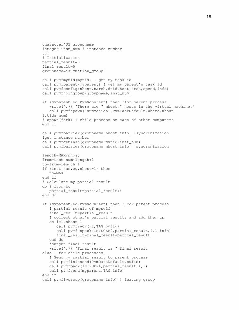
program summationimplicit noneinclude ‘fpvm3.h’integer nhost,mytid,myparentprocessor(process);final_result: final result of the summationinteger partial_result,final_result! length: the length of each block in the summation; from: the!beginning integer of each block; to: the ending integer of each!block.integer length,from,to! group name, each processor join the group to get the group instancenumber (from 0 to nhost-1)
18
character*32 groupnameinteger inst_num ! instance number...! Initializationpartial_result=0final_result=0groupname=’summation_group’
call pvmfmytid(mytid) ! get my task idcall pvmfparent(myparent) ! get my parent’s task idcall pvmfconfig(nhost,narch,dtid,host,arch,speed,info)call pvmfjoingroup(groupname,inst_num)
if (myparent.eq.PvmNoparent) then !for parent processwrite(*,*) “There are “,nhost,” hosts in the virtual machine.”call pvmfspawn(‘summation’,PvmTaskDefault,where,nhost-
1,tids,num)! spawn(fork) 1 child process on each of other computersend if
call pvmfbarrier(groupname,nhost,info) !syncronization!get instance numbercall pvmfgetinst(groupname,mytid,inst_num)call pvmfbarrier(groupname,nhost,info) !syncronization
length=MAX/nhostfrom=inst_num*length+1to=from+length-1if (inst_num.eq.nhost-1) then
to=MAXend if! Calculate my partial resultdo i=from,to
partial_result=partial_result+iend do
if (myparent.eq.PvmNoParent) then ! For parent process! partial result of myselffinal_result=partial_result! collect other’s partial results and add them updo i=1,nhost-1
call pvmfrecv(-1,TAG,bufid)call pvmfunpack(INTEGER4,partial_result,1,1,info)final_result=final_result+partial_result
end do!output final resultwrite(*,*) “Final result is “,final_result
else ! for child processes! Send my partial result to parent processcall pvmfinitsend(PvmDataDefault,bufid)call pvmfpack(INTEGER4,partial_result,1,1)call pvmfsend(myparent,TAG,info)
end ifcall pvmflvgroup(groupname,info) ! leaving group
19
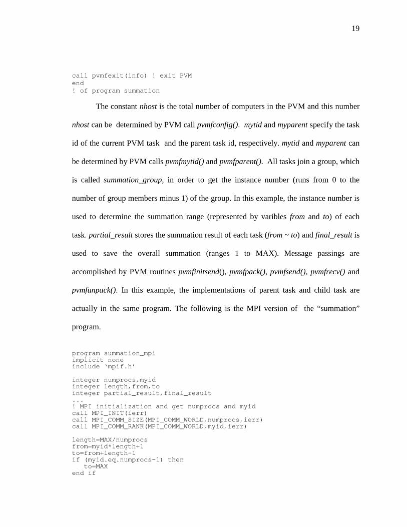
call pvmfexit(info) ! exit PVMend! of program summation
The constant nhost is the total number of computers in the PVM and this number
nhost can be determined by PVM call pvmfconfig(). mytid and myparent specify the task
id of the current PVM task and the parent task id, respectively. mytid and myparent can
be determined by PVM calls pvmfmytid() and pvmfparent(). All tasks join a group, which
is called summation_group, in order to get the instance number (runs from 0 to the
number of group members minus 1) of the group. In this example, the instance number is
used to determine the summation range (represented by varibles from and to) of each
task. partial_result stores the summation result of each task (from ~ to) and final_result is
used to save the overall summation (ranges 1 to MAX). Message passings are
accomplished by PVM routines pvmfinitsend(), pvmfpack(), pvmfsend(), pvmfrecv() and
pvmfunpack(). In this example, the implementations of parent task and child task are
actually in the same program. The following is the MPI version of the “summation”
program.
program summation_mpiimplicit noneinclude ‘mpif.h’
integer numprocs,myidinteger length,from,tointeger partial_result,final_result...! MPI initialization and get numprocs and myidcall MPI_INIT(ierr)call MPI_COMM_SIZE(MPI_COMM_WORLD,numprocs,ierr)call MPI_COMM_RANK(MPI_COMM_WORLD,myid,ierr)
length=MAX/numprocsfrom=myid*length+1to=from+length-1if (myid.eq.numprocs-1) then
to=MAXend if

20
do i=from,topartial_result=partial_result+I
end do
if (myid.eq.0) then ! for processor 0! add my partial resultfinal_result=partial_result! collect result from other processorsdo I=1,numprocs-1call
MPI_RECV(partial_result,1,MPI_INTEGER,MPI_ANY_SOURCE,TAG,MPI_COMM_WORLD,status,ierr)
final_result=final_result+partial_resultend do! output final resultwrite(*,*) “Final result is”,final_result
else ! for processor from 1 to numprocs-1! send my partial result to processor 0call MPI_SEND(partial_result,1,MPI_INTEGER,0,TAG,MPI_COMM_WORLD,&
ierr)end ifcall MPI_FINALIZE(rc) ! exit MPIend ! of program summation_mpi
myid and numprocs are the processor ID and the total number of processors in use. The
processor ID runs from 0 to numprocs-1 and can be efficiently used for the summation
program, as shown above. Messages passing are accomplished by MPI calls
MPI_SEND() and MPI_RECV(). For MPI, the number of processors used in the program
is decided by the command line parameter, for example, mpirun –np 8 summation means
that eight processors will be used in the parallel program.
3.3 Parallel Monte Carlo Simulation with Self-Scheduling Algorithm
To realize parallel computing in our Monte Carlo simulation of light propagating
through a tissue slab, we divide the photons in the incident beam into groups. Each group
of photons is assigned to one processor. If we allow these groups to be processed
concurrently by multiple processors, the parallel computing is achieved.

21
To make the code accessible and flexible, we design the parallel program for a
distributed computing environment consisting of different computers, and a self-
scheduling algorithm (master-slave) is used to coordinates the multiple processors. The
self-scheduling algorithm or master-slave mechanism is appropriate when the the slave
processes do not have to communicate with each another and the amount of work that
each slave must perform is difficult to predict [Gropp, 1999].
The simulation is composed of three independent but interactive processes: the
master process, the slave process, and the parallel random number generator
controller(PRNGC) process. To be more accurate, here we will use the term process
instead of program. The master process is the parent process for both slave and PRNGC.
It is the central control unit, and its responsibility consists of generating slaves and
PRNGC process, assgining tasks to slaves, collecting data, saving results and terminating
slaves and PRNGC. The very first step of the master process is to acquire some basic
information about the current distributed computing environment. These information
contains the total number of computers, computer names. Based on these information, the
master process is able to use the maximum available computing resouce to spawn slave
processes. After the spawning, usually one slave per computer with each spawning
followed by assigning a task to that slave, the master enters a loop. The body of the loop
consists of receiving result from whichever slave that just finished a task, then sending
the next to that slave. In other words, completion of one task by a slave is considered to
be a request for the next task. When a slave returns while master is running out of tasks, a
signal will be sent to terminate this slave. At the point when all tasks are finished, the

22
master process then terminates the PRNGC process, saves the results, and then ends the
simulation. Fig. 3.1 shows the relationship between the master, slave and PRNGC
processes.
3.4 PVM Implementation
In this section, we give a detailed explaination about our our parallel coding with
PVM interface. The flowchart shown in Fig. 3.2 gives the principle structure while the
correspoinding code is listed in Appendex B.1.
The first step of our master program is to include two header files: fpvm3.h and
param.h. fpvm3.h is the PVM header file for FORTRAN and it defines all the constants
which used for PVM library. param.h is our own header file, which specifies some of the
master
slave slave slave
PRNGC
Spawn
Spawn
Message Passing
Fig 3.1 In our parallel computing, photons in the incident beam are divided into groups (tasks). Different computer processes different task independently and concurrently. All tasks, which running on slaves, are controlled and coordinated by master. When finished, result of each task is reported back to master. Master thus collects all the results from these tasks and finally combines them to generate the final result. The combined result should be equivalent to the original sequential result.
23
frequently used constants and arrays in our simulation. NTASK describes the total
number of tasks we will have for the simulation. taskcount describes how many tasks
have already been assgined to slaves, and therefore it can indicate the current task
number. At the beginning, taskcount is initilized to zero. NR0 is a constant that is
frequently used in our program to describe the resolution of the radius of the circular
incoming beam area on the surface. It also means that the circle is divided into π(NR0)2
grids. At the initialization part, subroutine ChangeFromandTo() determines from and to
for the first task. Variables from and to specify the range one task will span at the
incoming beam area. For example, if NTASK is equal to one, from and to will span the
whole circular incoming beam area. Then the process enters the Clear to Zero part,
where all data arrays will be cleared to zero. Note that arrays with prefix Final are used to
save the final results. When we first call subroutine pvmfconfig(), argument nhost returns
with the number of computers in the current PVM. Then we make nhost-1 extra calls to
pvmfconfig() in order to extract a detailed list of computer information, say, hostnames
and DTIDs. Next, the master process begins to spawn PRNGC and all slaves. With
argument PVMTaskDefault in subroutine pvmfspawn(), PVM by itself chooses which
computer to spawn PRNGC. When spawning slaves, we use argument PVMTaskHost in
pvmfspawn(). Thus PVM is able to spawn slaves on the desired hostnames, which are
obtained earlier using pvmfconfig(). After spawning all processes, master stops and waits
for a respond from each slave. The message embeded in the slave’s respond includes only
the TID of that slave. task_tid is used here to store this TID number. A followed
pvmfgetinst() call returns the instance number of that slave in the whole slave group. The

24
name of the group(groupname) is specified as bmlaser in the Initialization part and the
instance number ranges from 0 to nhost-1. Each slave corresponds to one instance
number. Subroutine find_inst_from_dtid() assigns array tids and inst to make sure tids(i)
and inst(i) refer to the same computer. After all slaves respond, they are ready to receive
task parameters such as from, to and gen_tid. gen_tid is the TID of the PRNGC. master
sends each slave these parameters via pvmfinitsend(), pvmfpack() and pvmfsend(). As
taskcount is increasing, from and to are adjusted correspondingly. Afterwards, the master
enters its self-scheduling loop. At the beginning of the loop, we call pvmfrecv() to receive
result from any slave. Since pvmfrecv() is a blocking receive, master just stops and waits
until it receives a result from any slave. The received message is then unpacked and
saved in the intermedia arrays. These intermedia arrays are then added to the final arrays
in the following lines. Next, taskcount is compared with ntask. When taskcount is equal
to ntask, it means all tasks have been assigned and no more is available. At this case,
master specifies seed as zero in the message to make it a termination message. If
taskcount is less than ntask, master then assigns the returned slave another task. Finaly,
subroutine write_result_to_file() is called to save data files. This is the whole
implementation of the master with self-scheduling algorithm.
Each slave process begins with PVM calls pvmfparent() and pvmfmytid().
pvmfparent() returns the parent TID and pvmfmytid() returns its own TID. pvmfconfig() is
used to return nhost , which is the total number of computers in the current PVM. All
slaves then join the same group bmlaser by calling pvmfjoingroup(). Next, slave sents its
TID to master and call pvmfbarrier() to make sure all the slaves have joined the bmlaser

25
group. slave then enters a loop. At the beginning of the loop, slave calls pvmfrecv() and
pvmfunpack() to receive arguments, eg. from and to, from master. If it is a termination
signal (seed=0), slave steps out of the loop and ends. Otherwise, it calls simulation() to
run the task that specified with from and to. The results returned with simulation() are
then send to master.
3.5 MPI Implementation
In this section, we give a detailed explaination about our our parallel coding with
MPI interface. The flowchart is shown in Fig. 3.3 while the correspoinding code can be
found in Appendex B.2.
In our MPI implementation, the code for process master, slave and PRNGC are
combined into one program. Our MPI code is also based on the self-scheduling
algorithm, but for simplicity we didn’t use dynamic task allocation as that in the PVM
code. The processor number (myid) for each computer determines which actual process
(master, slave or PRNGC) will be run. For example, computer with processor number 0
runs the master process, computer with processor number numprocs-1 runs PRNCG and
computers with processor number 1 to numprocs-2 will be running slave. Each computer
can have more than one processes, with one processor number corresponds to one
process. For example, let’s assume we have 10 computers and on the command line we
use mpirun –np 21 mpi_control to start our MPI program. Once the program is running,
master will be running on computer with processor number 0. PRNGC will be running on
computer with processor number 20. As we only have 10 computers, the master, PRNGC
and one slave process are actually running on the same computer, with processor number

26
0, 10, 20, respectively. The implementations for master, slave and PRNGC are almost as
the same as the PVM implementation.
27
Begin
Initialization and GetPVM information
Spawn nhost tasks on nhostcomputers send them task
parameters
Collect results fromslaves and assign new
tasks
Combine results and save
End
Begin
Send TID to master
Receive taskparameter from
master
Seed=0?
Simulation(from,to,..)
Send result to master
End
Yes
No
Master process Slave process
PRNGC
Fig. 3.2 Flowchart for PVM implentations

28
Begin
Initialization
call MPI Comm rank(..,myid,..)
myid=0?
Yes
Enters masterprocess
Simulation(from,to)
Wait and receive resultfrom slaves
Combine results andsave
End
No
myid=numpocs-1?
Yes
Enters PRNGC process
End Enters slaveprocess
Simulation(from,to)
Send result tomaster
End
No
PRNGC
Fig. 3.3 Flowchart for MPI implentations

29
3.6 Parallel Computing Network
To facilitate our parallel computing needs, a 32-node workstation cluster with a
dual-CPU server has been established. For the workstations, we use PCs with Pentium
Celeron® CPU each at 433~500 MHz. The server has two Pentium® III CPUs with each
at 600 MHz. The combined peak performance is over 16Gflops (1 Gflops= 1*109
floating-point operations per second) and combined hard disk storage exceeds 190 GB.
The workstations are connected via a high-speed network with a maximum transmission
rate at 100M bits/sec so that the message-passing overhead for our parallel Monte Carlo
calculation is negligible.
Begin
Initialize seeds,indexes and spaces
Waiting for requestsfrom slaves
Send the currentindex to this slave
Fig. 3.4 Flowchart for PRNGC

30
basic
all the
share
availa
77/90
paralle
for de
Server
Client Client Client Client
High Speed Network
Fig. 3.5 The architecture of our workstation cluster and server. Theserver shares its resources with workstations via NFS.
The operating system we use for both server and clients is Red Hat Linux. The
architecture of our workstation cluster is shown in Fig 3.5. In our network design,
software packages and user account resources are on the server and workstations
these resources via NFS (Network File System). The current software resources
ble to the users are FORTRAN 77, C and C++ compilers from GNU, FORTRAN
and HPF (High Performance FORTRAN) from Portland Group, MPI and PVM
l computing interface libraries, and SPRNG libraries. Please refer to Appendix A
tails about the system installation, setup and administration.
4. Random Number Generator
In the Monte Carlo simulation of tissue scattering, there are many random
processes where random numbers are needed, such as determining the total distance of
photon’s propagation, the distance between each scattering and the propagation direction
after each scattering. Therefore, the properties of a random number generator (RNG) are
crucial to our simulation. In this chapter, we will first give a brief discussion on the basic
algorithms for both serial RNG and parallel RNG, and then present our implementations
of parallel RNG and associated statistical testing results in detail.
4.1 Sequential Random Number Generator Algorithms
The most commonly used random number generators are Linear Congruential
Generator (LCG) [Lehmer, 1949] and Lagged Fibonacci Generator (LFG) [Knuth, 1981].
LCG is often referred to as the Lehmer generator in the early literature. The linear
recursion underlying LCGs is:
Xn = a Xn-1+b (mod m) (4.1.1)
where m is called modulus, and a and c are positive integers called multiplier and
increment, respectively. The recurrence will eventually repeat itself, with a period that is
obviously no greater than m. If m, a and c are properly chosen, the period will be reach
maximal length as m. In this case, all possible integers between 0 and m-1 occur at some
point, so any initial “seed” choice of X0 is as good as any other.
The LCG has the advantage of being very fast, requiring only a few operations
per call, hence its almost universal use. It has the disadvantage that it is not free of
32
sequential correlation on successive calls. If k random numbers at a time are used to plot
points in k dimensional space, then the points will not tend to fill up the k-dimensional
space, but rather will lie on (k-1)-dimensional planes. There will be at most about m1/k
such planes. If the constants m, a and c are not very carefully chosen, there will be even
fewer than m1/k. LCGs also have the weakness of having their low-order (least significant)
bits much less random than their high-order bits [Press, 1992].
LFGs becomes increasing popular since they can offer a simple method for
obtaining sequence of very long periods. The recursion relation of a LFG can be
described as:
Xn = Xn-p Θ Xn-q (4.1.2)
where p and q are lags, and Θ is any binary arithmetic operation, such as addition,
multiplication and bitwise exclusive OR function (XOR). It is important that the
parameters p, q and Θ be carefully chosen in order to provide good randomness
properties and the largest possible period. Increasing the lags can improve the
randomness properties of the generator. Empirical tests have shown that when
multiplication is used, LFG has the best randomness properties., with addition (or
subtraction) being next best, and XOR being by far the worst.
When combining two different RNGs together, in many circumstances, we can
achieve an improved random number sequence. For example, L'Ecuyer [L'Ecuyer, 1993]
has shown how to additively combine two different 32-bit LCGs to produce a generator
that passes all known statistical tests and has a long period of around 1018, thus
overcoming the major drawbacks of standard 32-bit LCGs [NHSE Review, 1996].

33
4.2 Parallel Random Number Generator Algorithms
The basic idea under many parallel random number generators is to parallelize a
sequential generator by taking the elements of the sequence of pseudo-random numbers it
generates and distributing them among the processors in some way. An ideal parallel
random number generator should have the following qualities: 1. There should be no
inter-processor correlation. 2. Sequences generated on each processor should satisfy the
qualities of serial random number generators. 3. It should work for any number of
processors. 4. There should be no (or large size) data movement between processors.
To parallelize a sequential RNG, in general, there are three approaches: sequence
splitting, leapfrog and independent sequence. In the sequence splitting method, a serial
random number sequence is partitioned into non-overlapping contiguous section and each
section is assigned to one processor. For example, if the length of each section is L, the
random number subsequence for the pth processor will be:
XPL,XPL+1,XPL+2,…, (4.2.1)
Sequence splitting method requires a fast way to advance the serial sequence. But
a possible problem with this method is that although the sequences on each processor are
disjoint (i.e. there is no overlap), this does not necessarily mean that they are
uncorrelated. In fact it is known that LCG with modulus a power of 2 have long-range
correlations that may cause problems, since the sequences on each processor are
separated by a fixed number of iterations (L). Other generators may also have subtle long-
range correlations that could be amplified by using sequence splitting.
In the leapfrog method, the subsequence of the pth processor can be described as:

34
XP,XP+N,XP+2N,…, (4.2.2)
so that the sequence is spread across processors in the same way as a deck of cards is
dealt in turn to players in a card game. Leapfrog method again has the problem that long-
range correlations in the original sequence can become inter-processor correlations in the
parallel generator.
Independent sequence method is a simple way to parallelize a lagged Fibonacci
generator, which runs the same sequential generator on each processor, but with different
initial lag tables (or seed tables). In fact this technique is not different from what is done
on a sequential computer, when a simulation needs to be run many times using different
random numbers. In that case, the user just chooses different seeds for each run, in order
to get different random number streams. The initialization of the seed tables on each
processor is a critical part of this algorithm. Any correlations within the seed tables or
between different seed tables could have dire consequences. However this is not as
difficult as it seems - the initialization could be done by a combined LCG, or even by a
different LFG (using different lags and perhaps a different operation). A potential
disadvantage of this method is that since the initial seeds are chosen at random, there is
no guarantee that the sequences generated on different processors will not overlap.
However using a large lag eliminates this problem to all practical purposes, since the
period of these generators is so enormous that the probability of overlap will be
completely negligible.

35
4.3 Parallel RNG implementations for Monte Carlo Simulation
An appropriate RNG needed in our simulation must be able to generate a
sequence of random numbers satisfying statistical tests for randomness, uniformly
distributed in the full range from 0 to 1, not correlated, and have long period within the
acceptable error ranges. The implementation of the RNG should be easily ported to other
system.
4.3.1 Revised RNG RAN4
After careful study of many RNGs, we have adopted a RNG called RAN4 from
Numerical Recipes [Press, 1992] as the starting point for a portable parallel RNG. The
original RAN4 in Numerical Recipes only supports 32-bit system such that it has a
maximum period of 232. We extend it to support 64-bit integers in order to achieve a long
period of 264. Other modifications we made are: removed the initialization part of the old
RAN4 and increased the function’s argument number to two, one is idums and the other is
idum. idums is the initial seed and should keep unchanged all the time. idum is the index
number of the random sequence started from 1. Unless otherwise indicated, RAN4 in the
text below refers to the modified version.
RAN4 is based on the Data Encryption Standard (DES), and its implementation
consists of two parts. The first part of RAN4 is the DES encryption part, which basically
transforms one 64-bit integer into another 64-bit integer by doing bits shuffling and
mixing. The subroutine for this part is called psdes(), which is listed below,
SUBROUTINE psdes(lword,irword)implicit none

36
integer*8 irword,lword,NITERPARAMETER (NITER=4)integer*8 i,ia,ib,iswap,itmph,itmpl,c1(4),c2(4)
SAVE c1,c2DATA c1 /Z'BAA96887E171D32C',Z'1E17D32CAB9A6887',
+ Z'03BCDC3CF0331D2B',+ Z'0F33D1B2B40F85B3'/, c2 /Z'4B0F3B5878E4f3C0',+ Z'E874F0C35596A6C5',+ Z'6955C5A646AC55A7', Z'55A7CA464B0F3B58'/
do i=1,NITERiswap=irwordia=ieor(irword,c1(i))itmpl=iand(ia,Z'FFFFFFFF')itmph=iand(ishft(ia,-32),Z'FFFFFFFF')ib=itmpl**2+not(itmph**2)ia=or(ishft(ib,32),iand(ishft(ib,-32),Z'FFFFFFFF'))irword=ieor(lword,ieor(c2(i),ia)+itmpl*itmph)lword=iswap
end do
returnEND ! subroutine psdes
Compare with the original psdes() in Numerical Recipes, we extend the 32-bit
integers constants c1 and c2 to 64-bit and make sure each of them has 32 1-bits and 32 0-
bits. We also converse all 16-bit shift operation to 32-bit shift operation. The two
arguments - lword and irword - of psdes() are now both 64-bit integers, which are
defined as integer*8 in FORTRAN. The nonlinear function g [Press, 1992] is
implemented in the loop between do and end do ,and it consists of 64-bit integer
masking, shifting, mixing and multiplication. NITER is the total number of iterations, we
choose 4 here for NITER in order to make sure the generated random number sequence
has a good randomness properties. After all the multiplication and bits shuffling, we
obtain a 64-bit random number lword, which is also the output argument. In FORTRAN,

37
all integers are defined as signed integers, therefore the returned value lword must range
from –263 to 263-1.
The second part of RAN4, which manages data initialization and converting, is
shown below,
FUNCTION ran4(idums,idum)implicit none
real*8 ran4integer*8 idums,iduminteger*8 irword,lwordreal*8 twoto64
real*8 twoto64,tmp
twoto64=18446744073709551615.00
irword=idumlword=idumscall psdes(lword,irword)
tmp=irword*1.0
if (tmp.lt.0) thentmp=tmp+twoto64+1.0
end if
ran4=min(tmp/twoto64,1-(1e-18))ran4=max(tmp/twoto64,1e-18)
idum=idum+1
returnEND
Constant twoto64 equals to 264. The two arguments, idums and idum, go through
routine psdes() via temporary integers lword and irword. The output random number,
ranging from –263 to 263-1, is then saved again as irword and converted to a double
precsion number (real*8) spanning from 0 to 264. This number is further divided by 264
to normalize the number to the range between 0 and 1.

38
4.3.2 Sequence Splitting with RAN4
An extremelly useful feature of RAN4, is that it allows random access to the nth
random value in a sequence, without the necessity of first generating values 1 … n-1.
The nth random number can be easily acquired by calling function ran4(seed, n). This
property is shared by any random number generator based on hashing [Press, 1992].
Using this property, we can achieve a fast and efficient parallel RNG, with either
sequence splitting or leapfrog technique. In our implementation, we use the sequence
splitting method to separate the random number sequence (with a period of 264) into
equal-length sections. These sections are assigned on first come first serve basis.
Whenever a slave is running out of its sub-sequence, it will establish a connection to the
PRNGC to request a new one. In our implementation, PRNGC just send back the index and
length of next available sub-sequence to the applicant. The “real” random number is
actually generated by each slave process itself. The codes for PRNGC and the parallel
RAN4() are listed below,
program PRNGCimplicit noneinclude 'fpvm3.h'
integer RNGreq_tag,RNGreq_num,RNGsend_taginteger bufid,infointeger bytes,msgtag,tidinteger*8 index(1:6)integer seed(1:6)integer space(1:6)integer iinteger*4 index_h,index_linteger*8 tmp_index
!**********************! Initilization!**********************

39
RNGreq_tag=911RNGsend_tag=119
seed(1)=4984292seed(2)=83458335seed(3)=751608345seed(4)=126587347seed(5)=4326454seed(6)=1093732
space(1)=1000000space(2)=1000000space(3)=1000000space(4)=1000000space(5)=1000000space(6)=1000000
do i=1,6index(i)=1
end do
!**********************
do while (RNGreq_tag.eq.911)
!**************************! Get a request from a task!**************************
call pvmfrecv(-1,RNGreq_tag,bufid)call pvmfunpack(INTEGER4,RNGreq_num,1,1,info)call pvmfbufinfo(bufid,bytes,msgtag,tid,info)
!***************************************! Send that task a random number or seed!***************************************
call pvmfinitsend(PvmDataDefault,bufid)call pvmfpack(INTEGER4,seed(RNGreq_num),1,1,info)
! In case PVM doesn't support INTEGER8tmp_index=index(RNGreq_num)index_l=iand(tmp_index,Z'FFFFFFFF')index_h=iand(ishft(tmp_index,-32),Z'FFFFFFFF')call pvmfpack(INTEGER4,index_l,1,1,info)call pvmfpack(INTEGER4,index_h,1,1,info)
call pvmfpack(INTEGER4,index_l,1,1,info)call pvmfpack(INTEGER4,index_h,1,1,info)
!*** Reserved for dynamic space here ***call pvmfpack(INTEGER4,space(RNGreq_num),1,1,info)
call pvmfsend(tid,RNGsend_tag,info)

40
index(RNGreq_num)=index(RNGreq_num)+space(RNGreq_num)
end do
end ! of program PRNGC
The basic pricinple of the PRNGC is very straightforward. It keeps the initial seed
of the random number sequence and the current index as global variables to each slave.
The length of the sub-sequence is fixed as 1*107 in our program, but it can be adjusted
dynamically. Basically, what the PRNGC does is just staying there and waiting for requests
from slave processes. As soon as it receive a request, it assigns a new sub-sequence (or
block) to the slave applicant and sends back the current index. In our program, each
process needs more than one random number sequence (currently we need 6 random
number sequence for each process). The seeds and lengths for these random number
sequence are defined as array seed and array space, respectively. As PVM for Solaris, as
well as Red Hat Linux, supports only 32-bit integer (integer*4), the 64-bit index has to be
divided into two 32-bit integer and sent separately. One of the two 32-bit integer contains
the high order bits and the other contains the low order bits. At the recevier side, which is
in fuction ran4(), the two 32-bit integers are recomposed to generate the 64-bit index.
FUNCTION Get_RND_Num(which_one)
implicit noneinclude 'fpvm3.h'
external ran4_realreal*8 ran4_real
integer which_onereal*8 ran4integer gen_tidinteger RNGreq_tag,RNGreq_num,RNGrev_taginteger info,bufid

41
integer seed(1:6),space(1:6),count(1:6)integer*8 index(1:6)integer iinteger RNGreq_tag,RNGreq_num,RNGrev_taginteger*8 tmp_index,tmp_index0integer*4 index_l,index_h
common/generator/gen_tid
save seed,space,index
RNGreq_tag=911RNGrev_tag=119
if (which_one.lt.0) thenwhich_one=-which_onecount(which_one)=1
call pvmfinitsend(PvmDataDefault,bufid)call pvmfpack(INTEGER4,RNGreq_num,1,1,info)call pvmfsend(gen_tid,RNGreq_tag,info)
call pvmfrecv(gen_tid,RNGrev_tag,bufid)
call pvmfunpack(INTEGER4,seed(which_one),1,1,info)
! In case PVM doesn't support integer*8-----------call pvmfunpack(INTEGER4,index_l,1,1,info)call pvmfunpack(INTEGER4,index_h,1,1,info)
tmp_index0=index_htmp_index0=ishft(tmp_index0,32)
tmp_index=index_ltmp_index=ishft(tmp_index,32)tmp_index=ishft(tmp_index,-32)tmp_index=ior(tmp_index,tmp_index0)
index(which_one)=tmp_index!------------------------------------------------call pvmfunpack(INTEGER4,space(which_one),1,1,info)
end if
!*****************! PVM routines!*****************
if (count(which_one).lt.space(which_one)) thenran4=ran4_real(seed(which_one),index(which_one))index(which_one)=index(which_one)+1count(which_one)=count(which_one)+1
else

42
RNGreq_num=which_one
call pvmfinitsend(PvmDataDefault,bufid)call pvmfpack(INTEGER4,RNGreq_num,1,1,info)call pvmfsend(gen_tid,RNGreq_tag,info)
call pvmfrecv(gen_tid,RNGrev_tag,bufid)
call pvmfunpack(INTEGER4,seed(which_one),1,1,info)
! In case PVM doesn't support integer*8-----------call pvmfunpack(INTEGER4,index_l,1,1,info)call pvmfunpack(INTEGER4,index_h,1,1,info)
tmp_index0=index_htmp_index0=ishft(tmp_index0,32)
tmp_index=index_ltmp_index=ishft(tmp_index,32)tmp_index=ishft(tmp_index,-32)tmp_index=ior(tmp_index,tmp_index0)
index(which_one)=tmp_index!-------------------------------------------------call pvmfunpack(INTEGER4,space(which_one),1,1,info)
ran4=ran4_real(seed(which_one),index(which_one))index(which_one)=index(which_one)+1count(which_one)=1
end if
return
end
The function Get_RND_Num() is called by each process when it needs a random
number. Therefore, the inner mechanism for the splitting sequence and message passing
is totally transparent to the main simulation program. The main simulation program calls
Get_RND_Num(), knowning only the random number sequence (stream) number, which is
in turn represented by integer which_one in the range of 1 and 6. The Get_RND_Num()
function then determines the availability of current sub-sequence using a integer called

43
counter, when counter is less or equal than space, it means the current sub-sequence
still have random number unused. If counter is larger than space, a request is then made
to PRNGC, and the program waits for the next sub-sequence to be assigned and thus
determines the random number using the new index.
4.3.3 Testing Result of RAN4
To ensure the 64-bit RAN4 has the required statistical properties. We carried out
intensive statistic tests. Table 4.1 shows the testing results we obtained for RAN4 and
compared them with that of another RNG, RAN2 [Press, 1992]. RAN2 is a well tested
RNG provided by Numerical Recipes and it combines and shuffles two LCGs’ random
number sequences in order to break up serial correlations. In this way, RAN2 can reach a
period of 2*1018 [Press, 1992]. We didn’t use RAN2 for our parallel simulations because it
is not suitable for parallel computing.

44
T
s
r
o
v
b
r
u
i
Table 4.1 Statistic testing results for RAN4 and RAN2
RAN4 RAN2
Standard Deviation 131072.37888723 131072.37724003
Maximum Value 0.99999999987876 0.99999999987876
Minimum Value 2.2378115625745*10-10 2.2378115625745*10-10
Random Numbers in 0~1*10-6 9906(10000) 10071(10000)
in 1-1*10-6~1 10043(10000) 9953(10000)
Random Numbers in 0~1*10-9 8(10) 2(10)
in 1-1*10-9~1 11(10) 9(10)
he whole testing procedure is described below:
We made RAN2 and RAN4 each generate 1*1010 random numbers and divided the
pace between integers 0 and 1 into 100000 cells evenly. We want to see if the 1*1010
andom numbers are evenly distributed in those tiny cells in order to compare the results
f RAN2 and RAN4. Our tests consist of standard deviation test, maximum and minimum
alue test and counting the total random number belongs to our interested range.
We are concerned in the uniform distribution of the generated random numbers
etween 0-1, particularly near the ending regions, i.e. 0~1*10-8 and 1-1*10-8~1 because
andom numbers in those regions are crucial for us to determine the total number of
nattenuated photons in the transmitted light. For some RNGs, these regions are
nadvertently prohibited, which means that there is no or too few random numbers

45
existing in these regions. We must avoid this type of RNG in our simulation, as well as
those with random numbers not evenly distributed in the regions. Table 4.1 gives the
results for both RAN4 and RAN2. The values in the parenthesis are the expected values.
The testing suites in a parallel random number generator package, the SPRNG
(Scalable Parallel Random Number Generator Libraries from NCSA), are also employed
to test RAN4 with both sequential and parallel implementations. The testing suite includes
Gap test, Max of t test, Permutations test, Runs up test, Sum of independent distributions
test and Random-walk test. RAN4 passes all the tests in the suite and its results are
compared with the one of the well-tested RNGs, i.e. Comined Multiple Recursive
Generator in SPRNG and the results showed the same satisfying KS percentiles [Brock,
2000]. All these tests prove that RAN4 is a good RNG for both sequential and parallel
implementations.
4.3.4 Task Number Dependence
It has been well known that the result of parallel computing depend on its total
task number. In our Monte Carlo simulation, we also noticed that the results have
variations if using different number of tasks. Fig. 4.1 shows the difference in the light
distribution at the focal point along z-axis, between task number 20 and 10, with RAN4
and PVM. Fig. 4.2 shows the difference in the light distribution between task number 10
and 40, again with RAN4 and PVM.
To remove the possibility that the RNG of RAN4 causes this imperfection, we
employed one of the RNGs in SPRNG for a test simulation with the same parameters
used in Fig. 4.1. The result is presented in Fig. 4.3, it shows the similar characteristics of

46
task dependence as of that of Fig 4.1 where RAN4 was used. Therefore, we conclude that
the task-dependence is not due to the RAN4, but to the nature of parallel computing. In
the future, new approaches need to be developed to reduce this imperfection.
Fig. 4.1 Light distribution along the z-axis near the focal point for a convergingbeam incident on to a tissue slab. The solid line shows the result with 20 tasks, andthe dotted line shows the result with 10 tasks. In this simulation, µt=0.702, g=0.9,photon number=5.632*107. The simulation is accomplished with PVM and RAN4.
47
Fig. 4.2 Light distribution along the z-axis near the focal point for a converging beam incident on to a tissue slab. The curve with higher peak shows the resultwith 40 tasks, and the curve with lower peak shows the result with 10 tasks. Inthis simulation, µt=0.702, g=0.48, photon number=1.98*108. The simulation is accomplished with PVM and RAN4.
Fig. 4.3 Same as Fig. 4.1 except that it is calculated with a RNG of SPRNG using MPI.

5. Results and Discussions
In this chapter, we present the results of the parallel Monte Carlo simulation of a
converging light beam propagating through a slab of turbid medium. Particularly, we
studied light distribution near the focal point, dependence of the reflectance,
transmittance, and absorption of the incident light on the parameters µt and g, and
statistical distributions of the reflected and transmitted photons.
5.1 Light Distribution near Focal Point
As described in Chapter 2, we are interested in the distribution of the transmitted
light near the geometric focal point at z=Zf. For a cw converging Gaussian beam with N0
photons per unit time incident to a tissue slab of thickness D, according to Eq. 2.1.11, the
number of unttenuated photons in the transmitted light arriving at the focal point is given
by: [Wu, 2000]
2
01 2 0 0(1 )(1 )
2t D tt
uatt t
DwN R R N e N e dt
Fµ µ ∞− −− − − ∫ 5.1.1
where 0 2 / / 2tt F w Dw Fµ= + , and R1, R2 are the reflectivity at the entrance and exit
surfaces of the slab, respectively. For the cases we considered in this paper with F
=63mm and w = 4.86mm, we find F >> w, and therefore the second term in Eq. 5.1.1 can
be neglected. So we have
1 2 0(1 )(1 ) t DunattN R R N e µ−− − . 5.1.2
This provides the expected photon number peak at the focal point. Eq. 5.1.2 also
indicates that the coherent part of the incident radiance is attenuated exponentially with

49
the optical depth µt D. Thus, measuring of this peak against the slab thickness can lead to
the determination of the attenuation coefficient µt, or vice versa.
To study such dependence of the peak height on µt, we carried out simulations of
a converging laser beam propagating through a slab of diluted intralipid solution using
the parallel technique. Through the simulations, the slab thickness is fixed at D =17mm
while µt is changed from 0.546 (mm-1) to 1.092 (mm-1) through the variation of the
concentration of the solution slab. The optical parameters of intralipid solution are given
by an albedo (µs/µa) of 0.9666, and a refractive index n=1.33 and g=0.48 [Staveren,
1991]. We chose the transverse dimension of the slab in the xy-plane to be of
50mm×50mm to accommodate the simulation, and the parameters of the incident
Gaussian beam to have radius w = 4.86mm, cone angle α = 8.82o and focal length
F = 63mm. The unattenuated photons distribute along a spreading line in the z-axis
centered at z = Zf = 67.3mm, which is referred to as the focal point. The grid cells of the
deposit region are cubic with 50µm sides and the region occupies a (16mm)3 cube
centered at the focal spot.
Results for all the values of µt up to 1.09 (mm-1) show a well-defined peak formed
by the unattenuated photons at the focal point of the beam and a uniformly fluctuating
background around the peak. Because the photons of the incident beam are treated as a
spherical wave in our Monte Carlo simulations, the unattenuated photons propagates
toward the z-axis after emerging from the slab and form a peak at the focal point. This
peak in photon density has a significant width along the z-axis because of the aberrations
of the wavefront suffered at the plane interfaces of the slab while appear as a single point
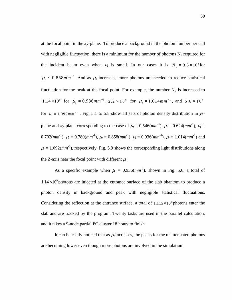
50
at the focal point in the xy-plane. To produce a background in the photon number per cell
with negligible fluctuation, there is a minimum for the number of photons N0 required for
the incident beam even when µt is small. In our cases it is 80 3.5 10N = × for
10.858t mmµ −≤ . And as µs increases, more photons are needed to reduce statistical
fluctuation for the peak at the focal point. For example, the number N0 is increased to
91.14 10× for 10.936t mmµ −= , 92 .2 1 0× for 11.014t mmµ −= , and 95 .6 1 0×
for 11.092t m mµ −= . Fig. 5.1 to 5.8 show all sets of photon density distribution in yz-
plane and xy-plane corresponding to the case of µt = 0.546(mm-1), µt = 0.624(mm-1), µt =
0.702(mm-1), µt = 0.780(mm-1), µt = 0.858(mm-1), µt = 0.936(mm-1), µt = 1.014(mm-1) and
µt = 1.092(mm-1), respectively. Fig. 5.9 shows the corresponding light distributions along
the Z-axis near the focal point with different µt.
As a specific example when µt = 0.936(mm-1), shown in Fig. 5.6, a total of
91.14 10× photons are injected at the entrance surface of the slab phantom to produce a
photon density in background and peak with negligible statistical fluctuations.
Considering the reflection at the entrance surface, a total of 91.115 10× photons enter the
slab and are tracked by the program. Twenty tasks are used in the parallel calculation,
and it takes a 9-node partial PC cluster 18 hours to finish.
It can be easily noticed that as µt increases, the peaks for the unattenuated photons
are becoming lower even though more photons are involved in the simulation.
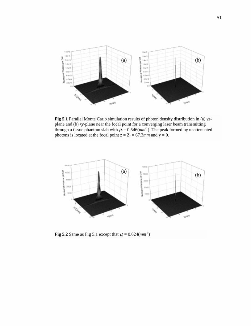
51
Fig 5.1 Parallel Monte Carlo simulation results of photon density distribution in (a) yz-plane and (b) xy-plane near the focal point for a converging laser beam transmitting through a tissue phantom slab with µt = 0.546(mm-1). The peak formed by unattenuated photons is located at the focal point z = Zf = 67.3mm and y = 0.
Fig 5.2 Same as Fig 5.1 except that µt = 0.624(mm-1)
(a) (b)
(a) (b)
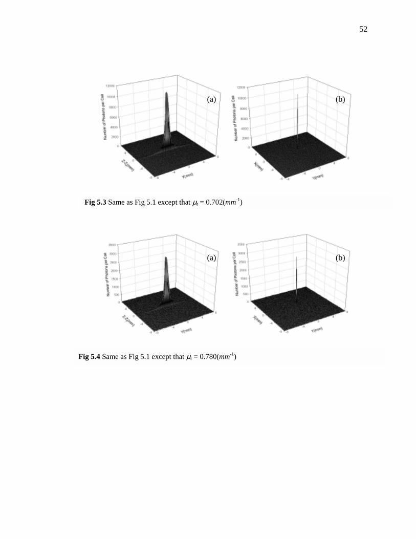
52
Fig 5.3 Same as Fig 5.1 except that µt = 0.702(mm-1)
Fig 5.4 Same as Fig 5.1 except that µt = 0.780(mm-1)
(b)
(b) (a)
(a)

53
(a) (b)
Fig 5.6 Same as Fig 5.1 except that µt = 0.936(mm-1)
Fig 5.5 Same as Fig 5.1 except that µt = 0.858(mm-1)
(a) (b)

54
Fig 5.7 Same as Fig 5.1 except that µt = 1.014(mm-1)
Fig 5.8 Same as Fig 5.1 except that µt = 1.092(mm-1)
(a)
(a)
(b)
(b)
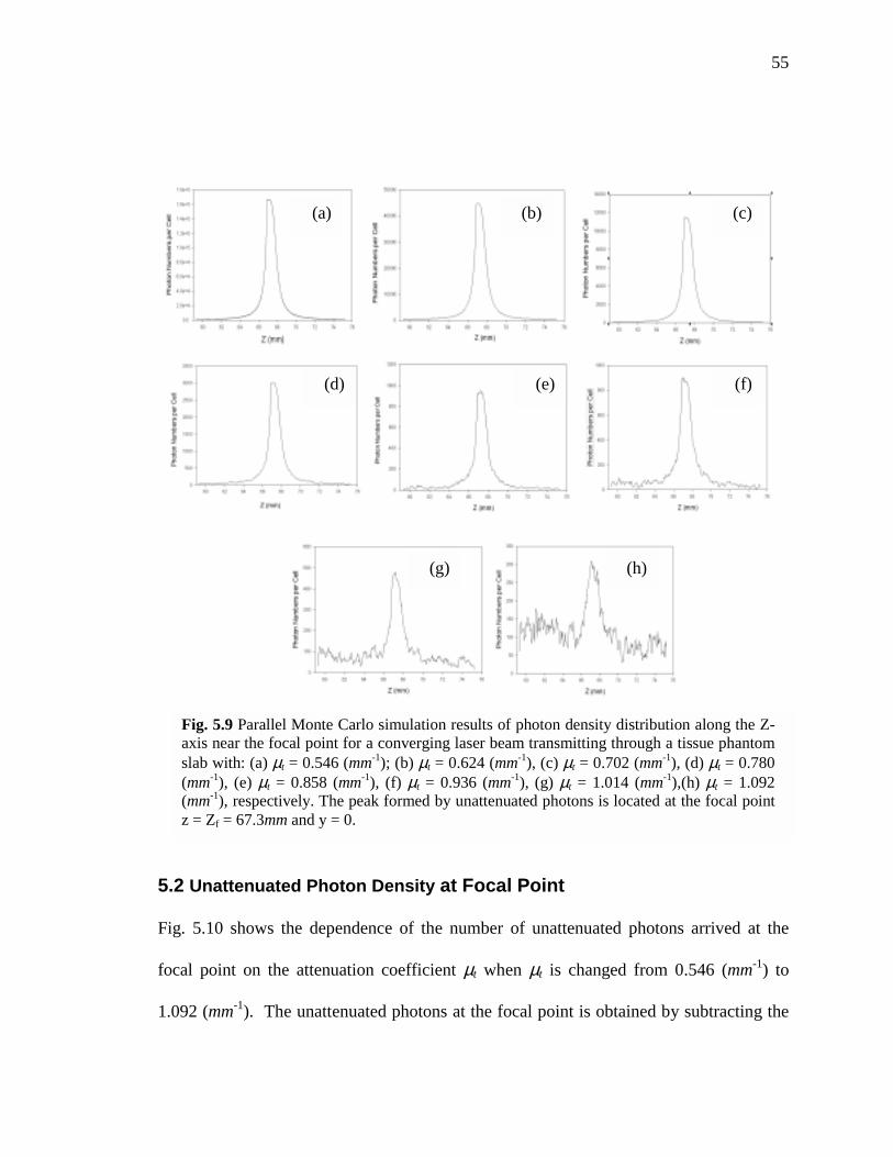
55
5.2 Unattenuated Photon Density at Focal Point
Fig. 5.10 shows the dependence of the number of unattenuated photons arrived at the
focal point on the attenuation coefficient µt when µt is changed from 0.546 (mm-1) to
1.092 (mm-1). The unattenuated photons at the focal point is obtained by subtracting the
Fig. 5.9 Parallel Monte Carlo simulation results of photon density distribution along the Z-axis near the focal point for a converging laser beam transmitting through a tissue phantom slab with: (a) µt = 0.546 (mm-1); (b) µt = 0.624 (mm-1), (c) µt = 0.702 (mm-1), (d) µt = 0.780 (mm-1), (e) µt = 0.858 (mm-1), (f) µt = 0.936 (mm-1), (g) µt = 1.014 (mm-1),(h) µt = 1.092 (mm-1), respectively. The peak formed by unattenuated photons is located at the focal point z = Zf = 67.3mm and y = 0.
(a) (b)
(h)(g)
(d) (e) (f)
(c)

56
background formed by the diffusely scattered photons from the observed peak. To do
that, we first obtain the photon density, or the number of photons per cell at the focal
point, Nf, from the light distribution deposition in the yz-plane, and Nf includes both
unattenuated and diffusely scattered photons. The diffusely scattered photon density Nb,
i.e. the background in the photon density near the focal point, is obtained by averaging
the number of photons per cell over the cells in the xy-plane excluding the single cell
where the peak is located. A simple treatment like this is well justified. First: the deposit
region is small enough so that the background is relatively flat. Second: due to the
geometric optical approximation adopted in the Monte Carlo simulation, all the
unattenuated photons are focused to a single cell in the xy-plane at z = Zf, so by excluding
that single cell, the xy-plane distribution is dominated by that of the diffusely scattered
Fig. 5.10 The dependency of unattenuated photons near the focal point on the ttenuate coefficient µt . The solid circles are the simulation results, while the straight is the predicted value from Eq. 5.1.2.

57
photons near the focal point. In this way we can obtain the unattenuated photons at the
focal point by Nunatt = (Nf − Nb) for each slab of µt. The results shown in Fig. 5.10 (solid
circle) are in excellent agreement with the radiative transfer theory prediction (the solid
line) given by Eq. 5.1.2. This proves directly that the photon density peak at the focal
point consists of the unattenuated photons on top of the diffusive background formed by
the multiply scattered photons.
The steep increase in the total number of tracked photon as a result of large
optical depth clearly demonstrates the urgent need to adopt the parallel computing
technique for conducting high performance computation in the biomedical optics.
5.3 Transmission, Reflection and Absorption
We also studied the dependence of the reflectance, transmittance, and absorption
of the incident light on the optical parameters µt and g.
We define the total number of reflected, transmitted, and absorbed photons as
Nreflct, Ntransm and Nabsorb, respectively, and the total photon number of incident photon as
N0, Fig. 5.12 shows the dependence of Nabsorb/N0, Ntransm/N0 and Nreflct/N0 on µt with
different g values. When attenuation coefficient µt is small, more photons will be
transmitted through the tissue slab. As µt increases gradually, more photons will be
absorbed inside the tissue. We also notice that Nreflct/N0 almost is constant as µt increases.
This characteristic fits different g value. Results show that large µt is associated with
large absorption and less transmission, but reflection is less sensitive to it.

58
Fig. 5.12 shows the dependence of Nabsorb/N0, Ntransm/N0 and Nreflct/N0 on g with
different µt values. While Ntransm/N0 increases with increasing g, Nreflct/N0 decreases as g
rises. For Nabsorb/N0, however, an interesting phenomenon is observed: it first increases as
g increases, but after it reachs certain point, Nabsorb/N0 begins to fall.
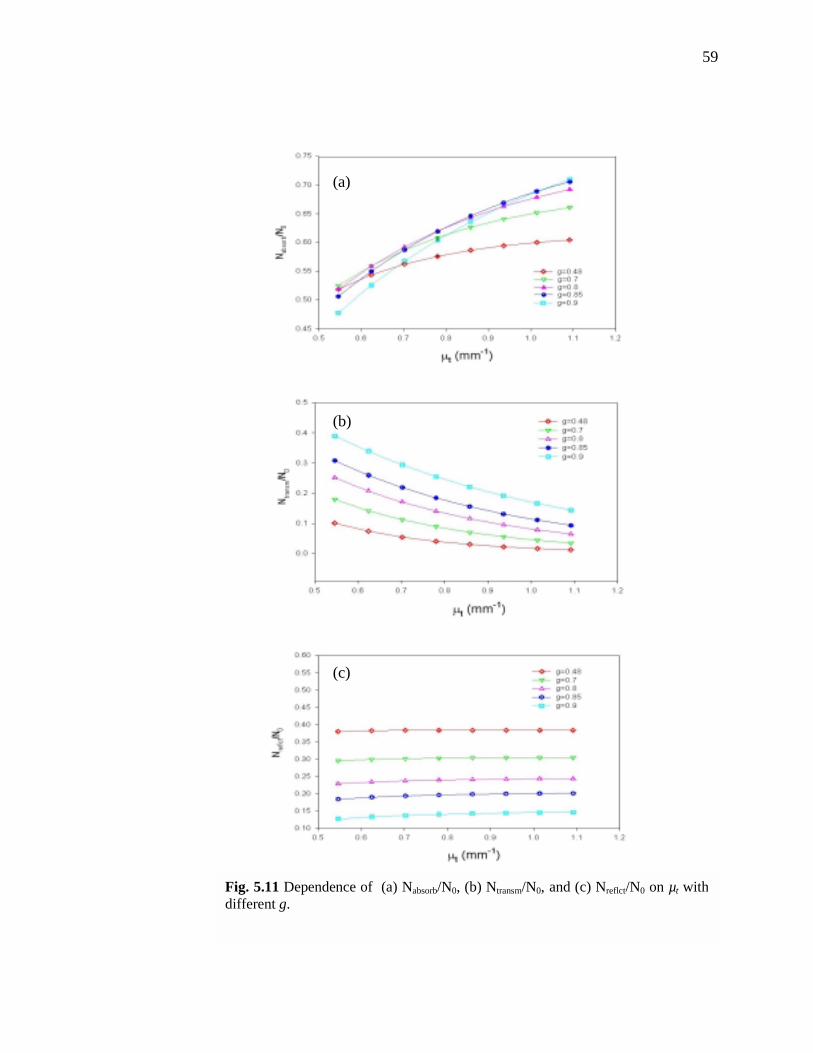
59
Fig. 5.11 Dependence of (a) Nabsorb/N0, (b) Ntransm/N0, and (c) Nreflct/N0 on µt with different g.
(a)
(b)
(c)

60
Fig. 5.12 Dependence of (a) Nabsorb/N0, (b) Ntransm/N0, and (c) Nreflct/N0 on g with different µt.
(a)
(b)
(c)

61
5.4 Scattering Statistics of the Reflected and Transmitted Photons
We have also looked into the statistical distributions of the reflected and
transmitted photons, and classified them according to the number of scatterings they have
experienced before they escape the tissue slab. For a given number of scatterings, the
observed number of photons at a given distance from the axis of the incident beam, i.e.
the radius ρ, in the focal plane for the transmitted photons or in the entrance plane for the
reflected photons are plotted in Figs. 5.14 and 5.13, respectively. A total of 5.6*107
photons participate in the both simulations with g=0.9 and µt=0.858. Other optical
parameters remain the same as described in Chapter 2.2.
We can see from Figure 5.14 that the distributions of the number of photons vs
the radius in the focal plane for a given number of scatterings is very broad. We also
notice that photons encountering different number of scattering have different
distributions in the focal plane, and no matter how many times photons are scattered, the
peak will always occur at the focal point. We also notice that as scattering number
increases, the peak will first move higher and then lower down, and photons with about
15 scatterings have the highest peak. That means most transmitted photons have been
scattered about 15 times.
In Figure 5.13, we notice that the distributions of the number of photons vs the
radius in the focal plane for a given number of scattering are much narrower than that in
Figure 5.14. The curves for fewer scatterings move higher as the number of scatterings
increase and reach the maximum for 5 scatterings and then drops quickly as the number
of scatterings increases more. That means, reflected photons are concentrated near the
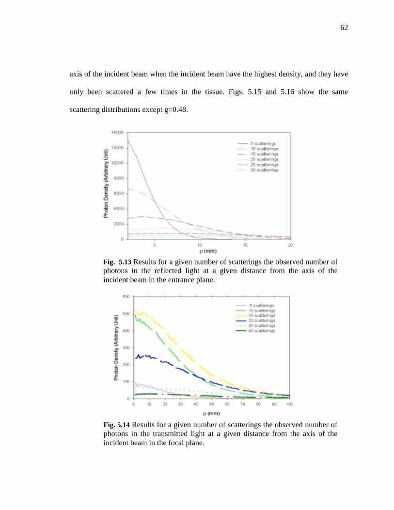
62
axis of the incident beam when the incident beam have the highest density, and they have
only been scattered a few times in the tissue. Figs. 5.15 and 5.16 show the same
scattering distributions except g=0.48.
Fig. 5.13 Results for a given number of scatterings the observed number ofphotons in the reflected light at a given distance from the axis of the incident beam in the entrance plane.
Fig. 5.14 Results for a given number of scatterings the observed number ofphotons in the transmitted light at a given distance from the axis of theincident beam in the focal plane.

63
Fig. 5.15 Same as Fig. 5.13 except g=0.48.
Fig. 5.16 Same as Fig. 5.14 except g=0.48.

Chapter 6: Summary
We have carried out large-scale simulations of a converging laser beam propagating
through a turbid medium of intralipid solutions using parallel Monte Carlo methods.
Through this research project, we constructed a 32-node UNIX cluster to provide a
powerful parallel computing environment and successfully converted previous sequential
codes into parallel codes using both MPI and PVM parallel computing interface software
packages. In addition, various random number generating algorithms were carefully
studied and a portable parallel random number generator has been developed for our
simulations. The outcomes of this research project provide a powerful tool for efficiently
executing large-scale simulations with low cost in the near future to model light-tissue
and light cell interactions.
The parallel computing cluster, including a dual-processor server and 32 client PCs,
was built on a LAN running on the LINUX operating platform. A server-client model
was employed where all the clients share the resources on the server. A portable random
number generator (RNG) has been developed for our parallel Monte Carlo simulations to
meet the special requirements for parallel computing and has been found satisfactory
through various statistical tests. In addition, RNGs from a well-tested random number
generator package, the SPRNG, were used to conduct the simulations for comparison
with those based on our own RNG, and they agreed well within the statistical error.
Parallel Monte Carlo codes have been developed to model a converging light beam
propagating through a tissue phantom in the form of slab using MPI and PVM on the
cluster environment based on previous sequential codes.[Song, 1999] The parallel
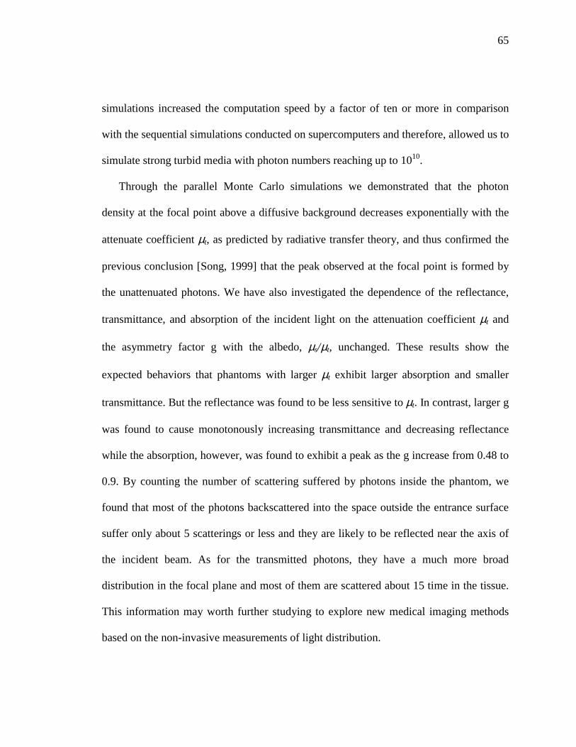
65
simulations increased the computation speed by a factor of ten or more in comparison
with the sequential simulations conducted on supercomputers and therefore, allowed us to
simulate strong turbid media with photon numbers reaching up to 1010.
Through the parallel Monte Carlo simulations we demonstrated that the photon
density at the focal point above a diffusive background decreases exponentially with the
attenuate coefficient µt, as predicted by radiative transfer theory, and thus confirmed the
previous conclusion [Song, 1999] that the peak observed at the focal point is formed by
the unattenuated photons. We have also investigated the dependence of the reflectance,
transmittance, and absorption of the incident light on the attenuation coefficient µt and
the asymmetry factor g with the albedo, µs/µt, unchanged. These results show the
expected behaviors that phantoms with larger µt exhibit larger absorption and smaller
transmittance. But the reflectance was found to be less sensitive to µt. In contrast, larger g
was found to cause monotonously increasing transmittance and decreasing reflectance
while the absorption, however, was found to exhibit a peak as the g increase from 0.48 to
0.9. By counting the number of scattering suffered by photons inside the phantom, we
found that most of the photons backscattered into the space outside the entrance surface
suffer only about 5 scatterings or less and they are likely to be reflected near the axis of
the incident beam. As for the transmitted photons, they have a much more broad
distribution in the focal plane and most of them are scattered about 15 time in the tissue.
This information may worth further studying to explore new medical imaging methods
based on the non-invasive measurements of light distribution.

References
1. Abrahams, P. , Larson, B. R , “Unix for the Impatient (Second Edition)” (1998)
2. Brock, R. S., “Testing random number generators with the Scalable Parallel
Random Number Generator (SPRNG) test suite” (2000).
3. Carriero, N. and Gelernter, D., “How to write parallel programs”, ACM
computing Surveys, Vol. 21(3), 323-356 (1989).
4. Chandrasekhar, S., Radiative Transfer, Oxford University Press, London (1960).
5. Das, B. B., Liu, F., Alfano, R. R., “Time-resolved fluorescence and photon
migration studies in biomedical and model random media”, Rep. Prog. Phys.,
Vol. 60, 227-292 (1997).
6. Dong, K., “Monte Carlo Simulation of Converging Laser Beams Propagating in
the Skin Tissue Phantoms with Random Rough Surfaces” (1999).
7. Fishman G. S., “Monte Carlo Concepts, Algorithms and Applications”, Springer-
Verlag, (1996).
8. Gardner, C. M., Jacques, S. L. and Welch, A. J., “Light Transport in Tissue:
Accurate Expressions for One-Dimensional Flounce Rate and Escape Function
Based Upon Monte Carlo Simulation,” Lasers in Surgery and Medicine, Vol. 18,
129-138 (1996).
9. Geist, A. , Beguelin, A. , Dongarra, J. , Jiang, W. , Manchek, R. and Sunderam,
V., “PVM (Parallel Virtual Machine) A User’s Guide and Tutorial for Networked
Parallel Computing” (1994).
67
10. Gropp, W., Lusk, E., “Installation Guide to mpich, a Portable Implementation of
MPI” (1996).
11. Gropp, W., Lusk, E., Skjellum, A., “Using MPI - Portable Parallel Programming
with the Message-Passing Interface second edition” (1999).
12. Henyey, L. G., Greenstein, J. L., “Diffuse radiation in the galaxy,” Astroph. J.,
Vol. 93, 70-83 (1941).
13. Ishimaru, A., “Wave Propagation and Scattering in Random Media”, Vol.1 and
Vol.2 (Academic, New York, 1978).
14. Johnson, C.C., “Optical diffusion in blood,” IEEE Trans. Biomed. Engineer., Vol
17, 129-134 (1970)
15. Keijzer, M., Jacques, S.T., Prahl, S.A., Welch, A.J., “Light distribution in artery
tissue: Monte Carlo simulation for finite-diameter laser beams,” Lasers Surg.
Med., Vol. 9, 148-154 (1989).
16. Knuth, D.E., “The Art of Computing Programming Vol. 2: Seminumerical
Methods (second edition)”, Addision-Wesley, Reading, Mass. (1981).
17. Kochan, S. G. and Wood, P. H., “UNIX Networking” (1989).
18. Kochan, S. G., “UNIX Shell Programming, Revised Edition” (1993).
19. L'Ecuyer, P., Blouin, F., and Couture, R., A search for good multiple recursive
generators, ACM Trans. on Modeling and Computer Simulation, Vol. 3, 87
(1993).
20. Leffler, S. J., Mckusick, M. K, Karels M. J. and Quarterman, J. S., “The Design
and Implementation of the 4.3BSD UNIX Operating System” (1989)

68
21. Lehmer, D.H., “Mathematical methods in large-scale computing units,” in Proc.
2nd Symposium on LargeScale Digital Calculating Machinery, Harvard University
Press: Cambridge, Massachusetts,141-146 (1949).
22. Lu, J. Q., Hu, X. H., Song, Z. and Dong K., “Simulation of Light Scattering in
Biological Tissues: the Coherent Component.”, Vol. 3601, SPIE Proceeding,
being published (1999).
23. Mascagni, M., Ceperley D. and Srinivasan, A., “SPRNG: A Scalable Library for
Pseudorandom Number Generation” (1998).
24. Miller, I. D. and Veitch, A.R., “Optical Modeling of Light Distributions in Skin
Tissue Following Laser Irradiation,” Lasers in Surgery and Medicine, Vol. 13,
565-571 (1993).
25. NHSE Review, “Random Number Generator for Parallel Computers” (1996).
26. Press, W. H., Teukolsky, S. A., Vetterling, W. T. and Flannery, B. P.,
“Numerical Recipe in C ( Second Edition)”, Chapter 7, (1992) .
27. Snir, M., Otto, S., Lederman, S. H., Walker, D. and Dongarra, J., “MPI – The
Complete Reference, Volume 1, The MPI Core (Second Edition)” (1998).
28. Song, Z., Dong, K., Hu X. H. and Lun, J. Q., “Monte Carlo Simulation of
Converging Laser Beams Propagating in Biological Materials”, Applied Optics,
Vol. 38, 2944-2949 (1999).
29. Staveren, H.J. van, Mose, C.J.M., Marle J. van, Prahl, S.A., Germert, M.J.C. van,
“Light scattering in intralipid-10% in the wavelength range of 400-1100 nm”,
Appl. Opt., Vol. 30, 4507-4514 (1991).

69
30. Stevens, W. R. , “Advanced Programming in the UNIX Environment” (1993)
31. van Gemert, M.J.C., Jacque, S. L., Sterenborg, H.J.C.M and Star, W. M., “Skin
optics,” IEEE Trans. Biomed. Eng., Vol. 36, 1146-1154(1989)
32. Wan, S., Anderson, R. R. and Parrish, J. A., “Analytical modeling for the optical
properties of the skin with in vitro and in vivo applications,” Photochem.
Photobiol. , Vol. 34, 493-499 (1981)
33. Wang, L. H., Jacques, S. L. and Zheng, L.Q., “CONV – Convolution for
responses to a finite diameter photon beam incident on multi-layed tissues,”
Comp. Meth. Prog. Biomed., Vol 54, 141-150 (1997).
34. Wang, L. H., Jacques, S. L. and Zheng, L.Q., “MCML – Monte Carlo modeling
of light transport in multi-layered tissues,” Comp. Meth. Prog. Biomed., Vol. 47,
131-146 (1995).
35. Wilson, B.C. and Adams, G., “A Monte Carlo model for the absorption and flux
distribution of light in tissue,” Med. Phys., Vol. 10, 824-830 (1983).
36. Winsor, J., “Advanced System Administrator’s Guide, Second Edition” (1998).
37. Wu, D., Zhao, S. S., Lu, J.Q., Hu, X.H., “Monte Carlo Simulation of Light
Propagation in Skin Tissue Phantoms Using a Parallel Computing Method,”,
Proceedings of SPIE, being published. (2000)