parabolic obstacle problems applied to finance - department of

PARABOLIC OBSTACLE PROBLEMS APPLIED TO FINANCEA FREE-BOUNDARY-REGULARITY APPROACH

ARSHAK PETROSYAN AND HENRIK SHAHGHOLIAN

Abstract. The parabolic obstacle problem within financial mathematics isthe main object of discussion in this paper. We overview various aspects ofthe problem, ranging from the fully nonlinear case to the specific equations inapplications. The focus will be on the free boundary and its behavior close toinitial state, and the fixed boundary. In financial terms these can be translatedas the behavior of the exercise boundary for American option, close to maturityand close to the barrier.

From free-boundary-regularity point of view, such problems have not beenconsidered earlier.

1. Introduction

1.1. Background. The parabolic obstacle problem refers to finding the smallestsupersolution (for a given parabolic operator, and given domain and boundary data)over a given function (obstacle).

This problem appears in applications, such as phase transitions (melting andcrystallization), mathematical biology (tumor growth), and American type con-tracts in finance. Of obvious reasons, the latter application has gained grounds inthe recent past.

Although many financial problems involve linear equations, there are many re-lated problems with nonlinear governing equations, that require more delicate anal-ysis. It is our aim here to give an account of some new ideas and techniques, fornonlinear parabolic obstacle problem from free boundary regularity point of view.In doing so, we will present some general results describing the optimal regularityof the solutions as well as describing the behavior of the free boundary at initialstate and also close to a fixed boundary. These, general results are then exemplifiedin terms of applications in finance.

A highlight of this paper is the specific application of our results for the valuationof the American put option of minimum of two underliers, see last section.

1.2. Mathematical formulation. Let us denote by Q+ the upper-half of the unitcylinder in Rn+1, and let ψ(x, t) be parabolically C0,α.

Set

(1.1) H(u) = F (D2u,Du, u, x, t)−Dtu,

2000 Mathematics Subject Classification. Primary: 35R35.Key words and phrases. Free boundary, obstacle problem, global solution, blow-up, American

type contracts, payoff.A. Petrosyan is supported in part by NSF grant DMS-0401179. He also thanks the STINT

Foundation for supporting his visit to Royal Institute of Technology in Stockholm, Sweden.H. Shahgholian is supported by Swedish Research Council.

1

2 ARSHAK PETROSYAN AND HENRIK SHAHGHOLIAN

where F is a fully nonlinear uniformly elliptic operator with certain homogeneityproperties for which the regularity theory of viscosity solutions [Wan92a, Wan92b,Wan92c] applies. For more precise assumptions on F , see Section 1.3 in [Sha06].Let u solve the parabolic obstacle problem

(1.2) (u− ψ)H(u) = 0, u ≥ ψ in Q+,

(1.3) H(u) ≤ 0,

with boundary datum

(1.4) u(x, t) = g(x, t) ≥ ψ(x, t) ∂pQ+.

(Here the notation ∂p stands for the parabolic boundary, see [Wan92a].)Let us set

E(u) = (x, t) ∈ Q+ : u(x, t) = ψ(x, t),C(u) = (x, t) ∈ Q+ : u(x, t) > ψ(x, t).

The obstacle ψ in general has singularities, usually representing a change in thenature of the contract in applications in finance. It should be remarked that inthe applications in this paper we exclusively consider the American put option.Examples of obstacles that appear in finance are given below (here E is a constantand it denotes the exercise price).

Obstacle ψ Applications

(E − x1)+ 1-d contract, American putmin(E − x1)+, (E − x2)+ min option, American put.

Another type of contract that also is of interest in the market is that of barriertype options, referring to termination/start of a contract, before the time of matu-rity. Here we will also discuss this issue from the obstacle problem point of view.However, we will only consider the case of down-and-out barriers (termination of acontract with a rebate) for American put option.

1.3. Smooth obstacles. For the smooth obstacle case, there is a vast literaturetreating various aspects such as existence and regularity of the solutions, as wellas certain geometric inheritance. In the linear case one can even make a furthersimplification of the problem by considering the function U = u−ψ, and after somestandard analysis one comes to the conclusion that

(1.5) H(U) = fχU>0, U ≥ 0,

where f = −H(ψ), and the free boundary is now ∂U > 0.The study of the obstacle problem, in one dimension and in the case of Ste-

fan problem ∂tU ≥ 0 (which is a result of specific data, e.g. if the obstacle istime-independent) has been successfully carried out by several people; see [Fri75],[vM74a, vM74b].

In higher dimensions, besides existence theory and some partial results on ge-ometry, there are hardly any other results. Concerning the regularity of the freeboundary, the only known general result is [CPS04]. For the case of Stefan problem

PARABOLIC OBSTACLE PROBLEM 3

see also [Caf77]. Although both these papers treat the Laplacian case, one caneasily generalize part of the results to more general, but still linear, operators. Cf.also a recent paper by Blanchet et al. [BDM05].

1.4. Non-smooth obstacles. When the obstacle is non-smooth, even in the sim-ple Laplacian case, one can not reformulate the problem into (1.5) and hence thereare not many know techniques to be used in the study of the obstacle problem. Ofcourse, even if the obstacle is smooth, but the operator is non-linear, then we stillare in situation that earlier techniques are not applicable. A complete study of theproblem is yet to come.

In this note we will present some results for the non-smooth case, with focus onapplications to American type options in finance.

2. Applications to Finance and Optimal Stopping

The above obstacle problem, appears naturally in the valuation of American typeclaims, in financial market. The obstacle is the so-called payoff function and theoptimal configuration u is the value of the option. For a good background studywe refer the reader to the paper by M. Broadie and J. Detemple [BD97].

Let us denote St = (S1t , S

2t ) to be the price vector of underlying assets at time

t. The price Sit follows the standard Brownian motion

dSit = (r − δi)Si

tdt+ σidWit , i = 1, 2

where r is the constant interest rate, δi is the dividend rate of the i-th stock, and σi

is the volatility of the price of the corresponding asset. The notation W it also stands

for the standard Brownian motion, over a probability filtered space (Ω,F , P ), withP as the risk-neutral measure.

The value function V of the American option is given by

(2.1) V (S, t) = supτE

(e−r(T−t)ψ(Sτ )

)

with the stopping time τ varying over all Ft-adapted random variables, and ψ(S)the option payoff. Here (Ft)t≥0 denotes the P completion of the natural filtrationassociated to (W i

t )t≥0. This completion comes from the so-called completeness ofmarkets, so that one has a unique solution to the problem.

Stochastic analysis can now be used to show that V satisfies a variational in-equality, here written in the complementary form,

LV + ∂tV ≤ 0, (LV + ∂tV ) (ψ − V ) = 0, V ≥ ψ ,

a.e. on Rn × [0, T ) , and with condition

V (x, T ) = ψ(x, T ).

Here the elliptic operator L is given by

LV = (r − δ1)S1 ∂V

∂S1+ (r − δ2)S2 ∂V

∂S2+

+12

((σ1S

1)2∂2V

∂(S1)2+ σ1σ2S

1S2 ∂2V

∂S1∂S2+ (σ2S

2)2∂2V

∂(S2)2

)− rV .

The backward parabolic equation, can be turned into forward equation by achange of variable, and hence we arrive at the case of the parabolic obstacle problemin this paper.


In general, the obstacle ψ is non-smooth at some point x0, at time of maturityt = T . Examples of such obstacles can be found in [BD97].

3. Parabolic notation

For a point X = (x, t) ∈ Rn×R and r > 0, we consider three kinds of paraboliccylinders:

Qr(X) = Br(x)× (t− r2, t+ r2),

Q−r (X) = Br(x)× (t− r2, t], (lower cylinder)

Q+r (X) = Br(x)× [t, t+ r2). (upper cylinder)

When X = (0, 0) we don’t indicate the center. For a cylinder Q = B × I, where Iis an interval with endpoints a < b, then we define

∂xQ = ∂B × I, (lateral boundary)

∂bQ = B × a, (bottom)

∂pQ = ∂xQ ∪ ∂bQ (parabolic boundary)

ForX = (x, t) we denote |X| =√x2 + |t|. Then |X−Y | is the parabolic distance

between X and Y .Given 0 < α ≤ 1, the parabolic Holder space C0,α(Ω) is defined as the subspace

of C(Ω) consisting of functions f such that the norms

‖f‖C0,α(Ω) = ‖f‖C(Ω) + supX,Y ∈Ω,X 6=Y

|f(X)− f(Y )|X − Y |α

are finite. Next, the parabolic spaces Ck(Ω) for integers k are defined as the spaceof continuous functions f for which the derivatives Di

xDjtf with |i| + 2j ≤ k are

also continuous, with appropriately defined norm. (Here i is a multi-index and j isan integer.) For integer k, 0 < α ≤ 1, and f ∈ C(Ω) let

[f ]k,α(X) = infPk

supr>0

1rα

supQ−r (X)∩Ω

|u− Pk|,

where Pk(X) =∑|i|+2j≤k ai,jx

itj are polynomials of parabolic order ≤ k. Thenthe higher parabolic Holder spaces Ck,α(Ω) are defined as the subspaces of Ck(Ω)consisting of functions f such that the norms

‖f‖Ck,α(Ω) = ‖f‖Ck(Ω) + supX∈Ω

[f ]k,α(X)

are finite.

4. Regularity of the solution

A compactness-based technique developed in [Sha06] allows to prove the follow-ing result, which essentially says that the solution of the obstacle problem is asregular as the obstacle, up to C1,1, similarly to the classical obstacle problem.

Theorem 4.1 (Optimal interior regularity). Let u be a solution to the obstacleproblem in Q−1 with obstacle ψ ∈ Ck,α

(Q−1

)for k = 0, 1 and 0 < α ≤ 1. Then

u ∈ Ck,αloc (Q−1 ) and for any K ⊂⊂ Q−1

‖u‖Ck,α(K) ≤ C(K,F, k, α, n, ‖u‖L∞(Q−1 ), ‖ψ‖Ck,α(Q−1 )

).


The next two results deal with the boundary regularity of the solutions.

Theorem 4.2 (Lateral boundary regularity). Let u be as in Theorem 4.1 withk = 0, 1, 0 < α ≤ 1, and boundary values g ∈ C2,ε(Q−1 ∪ ∂xQ

−1 ) for some ε > 0.

Then u ∈ Ck,αloc

(Q−1 ∪ ∂xQ

−1

)and for any K ⊂⊂ Q−1 ∪ ∂xQ

−1

‖u‖Ck,α(K) ≤ C(K,F, k, α, n, ε, ‖g‖C2,ε(Q−1 ∪∂xQ1), ‖ψ‖Ck,α(Q−1 )

).

Theorem 4.3 (Initial regularity). Let u be as in Theorem 4.1 and assume alsothat it takes boundary values g ∈ Ck,α(Q−1 ∪ ∂bQ1). Then there exists β = β(k, α),0 < β < 1 such that u ∈ Ck,β

loc (Q−1 ∪ ∂bQ−1 ) and for any K ⊂⊂ Q−1 ∪ ∂bQ

−1

‖u‖Ck,β(K) ≤ C(K,F, k, α, n, ‖g‖Ck,α(Q−1 ), ‖ψ‖Ck,α(Q−1 )

).

In applications to finance, where u represents the value function for a certainderivative, usually one can represent the u as the supremum of the expected valueover a class of stopping times. From such representations one can derive the optimalregularity of the solution by computations; cf. [CC03].

Sketch of the proof. The proof of Theorem 4.1 is an consequence from the fol-lowing growth estimate.

Lemma 4.4. Let u be as in Theorem 4.1 and assume that ‖u‖L∞(Q−1 ) ≤ 1,‖ψ‖Ck,α(Q−1 ) ≤ 1. Then there exists C = C(k, α, n) such that

supX∈Q−r (Z)

|u(X)− u(Z)| ≤ Crα, if k = 0

andsup

X∈Q−r (Z)

|u(X)− u(Z)−Dxψ(Z)(x− z)| ≤ Cr1+α, if k = 1,

for any Z = (z, s) ∈ ∂E(u) ∩Q−1/2 and 0 < r < 1/2.

The proof of this lemma is based on a compactness argument developed in[Sha06].

In the case k = 0 define

Sj = Sj(u,Z) = supX∈Q2−j (Z)

|u(X)− u(Z)|, j = 1, 2 . . . ,

for any point Z ∈ ∂E(u) ∩ Q−1/2. The statement of the lemma will follow once weprove that

Sj ≤ C2−αj , j = 1, 2 . . .for a universal constant C. The proof is by establishing the recursive relation

Sj+1 ≤ max

C

2−jα,Sj

2α,Sj−1

22α, . . . ,

S1

2jα

.

Assuming that this inequality fails for any value of C, we will have a sequence ofsolutions ui in Q−1 , i = 1, 2, . . ., with obstacles ψi as above, integer ki and a pointZi = (zi, si) ∈ ∂E(ui) such that

Ski+1 ≥ max

i

2−kiα,Ski

2α,Ski−1

22α, . . . ,

S1

2kiα

.


Then we consider the rescalings

ui(x, t) =ui(zi + 2−kix, si + 2−2kit)− ui(Zi)

Ski+1(ui, Zi), (x, t) ∈ Q−

2ki(−Zi).

It is easy to see that ui is a solution of the obstacle problem with appropriatelymodified obstacle ψi. Next, without loss of generality we may assume that Zi

converges to Z0 ∈ Q−1/2. Then ui are uniformly bounded in Q−1 and ψi → 0 locallyuniformly in Q−1 . Then a barrier argument can be used to show that

ui → 0 uniformly on Q−1/2.

However, this contradicts to the fact that

supQ−1/2

|ui(X)| = 1.

The proof in this case k = 1 follows the same scheme, except we need to redefine

Sj = Sj(u,Z) = supX∈Q2−j (Z)∩Q−1

|u(X)− u(Z)−Dxψ(Z)(x− z)|

and

ui(x, t) =ui(zi + 2−kix, si + 2−2kit)− ui(Zi)− 2−kiDxψ(Zi)x

Ski+1(ui, Zi)and establish that

Sj ≤ C2−(1+α)j , j = 1, 2, . . . .The proofs of Theorems 4.2 and 4.3 are little more involved as they require

boundary analysis, but also follow a similar scheme (see Theorem 1.3 in [Sha06]).

5. Regularity of the free boundary

In this section we discuss results concerning the regularity of the free boundary.The results are stated in the framework of fully nonlinear operators, however, someof the results are currently known only for the heat equation, while some others areknown for a fairly general class of operators.

5.1. Interior regularity for smooth obstacles.

Theorem 5.1 (Interior spatial regularity backward in time). Let u be a solutions ofthe obstacle problem, with ψ ∈ C∞(Q1). Suppose for some point Z ∈ ∂E(u)∩Q1/2,with H(ψ)(Z) = −c0 < 0, we have that the set

(5.1) E−r (u;Z) := E(u) ∩Q−r (Z)

is thick enough for some r = r1 in the sense that

δ−r (u;Z) :=|E−r (u;Z)||Q−r (Z)| > σ(r)

for a certain modulus of continuity σ. Then the free boundary ∂E is locally inQ−r0

(Z) a C1-graph in some of the space directions, and for some r0. Moreover, themodulus of continuity σ as well as r0 can be chosen uniformly for ψ in appropriatelydefined classes.

This result is currently known only for the heat operator, see [CPS04]. A relatedresult for a fully nonlinear elliptic obstacle-type problem can be found in [LS01].


Remark 5.2. We note here that the possibility of having “flat in time” free bound-aries as in the example

u(x, t) = −|x|2

2n+

(12− t

)+

, ψ(x, t) = −x2

2nfor the operator F = ∆ prevents from having the analogue of this theorem for for-ward in time spatial regularity of the free boundary. However, under the assumptionDtu ≥ Dtψ in Q1, which mathematically corresponds to the Stefan problem case,we can replace the thickness of E−r (u;Z) by that of

Er(u;Z) = E(u) ∩Qr(Z)

or even with the thickness of any of its t-cuts in Qr(Z) and obtain the spatialregularity of ∂E in Qr0(Z).

To illustrate the idea of the proof, we state here one of the intermediate steps inthe case F = ∆ in [CPS04].

Lemma 5.3 (Convexity of global solutions). Let w be a nonnegative solution of∆w −Dtw = c0χw>0 in Rn ×R− such that

|w(X)| ≤M(1 + |X|2), X ∈ Rn ×R−

for some constant M . Then Deew ≥ 0 for any spatial direction e and Dtw ≤ 0. Inparticular, the t-slices

E(t) = x : w(x, t) = 0are convex and shrink as t decreases.

The proof of this lemma is based on the following argument. Assuming thatDeew is negative at some points, we take a minimizing sequence Xn such that

Deew(Xn) → m = infw>0

Deew < 0.

Note that m is finite by the optimal regularity theorem (see Theorem 4.1 above).Then consider the rescalings

wn(X) =1d2

n

w(xn + dnx, tn + d2nt),

were dn is the parabolic distance of the point Xn to the coincidence set w = 0.Over a subsequence, wn will converge to a solution w0 of ∆w0−Dtw0 = c0χw0>0in Rn ×R−, which will have the following properties:

∆w0 −Dtw0 = 1 in Q−1 , Deew0(0, 0) = minQ−1

Deew0.

The function v = Deew itself will satisfy the heat equation in Q−1 and therefore bythe minimum principleDeew = m = const in Q−1 . Moreover, this equality continuesto hold in the parabolic connected component of the set w > 0. Assuming thate = e1, this implies the representation

w0(x1, 0, . . . , 0) =m

2x2

1 + bx1 + c

for some constants b and c, which will hold at least for 0 < x1 < 1 and will continueto hold as long as w0 > 0. However, since m < 0 there will be the first x1 = x∗1,where w0 will become 0. This will imply the representation

w0(x1, 0, . . . , 0) =m

2(x1 − x∗1)

2, 0 < x1 < x∗1,


since both w0 and D1w0 should vanish at x1 = x∗1. However, this contradict tononnegativity of w, as m < 0.

A similar argument proves also that Dtw ≤ 0.

5.2. Behavior near the fixed boundary.

Theorem 5.4 (Touch with the fixed boundary). Let u be a solutions of the obstacleproblem in Q1 with ψ, g ∈ C∞(Q1). Suppose for a boundary point Z = (z, 0) withz ∈ ∂B1 and Hψ(Z) < 0, we have that Z ∈ ∂E, i.e. there exists Zj → Z withZj ∈ C(u). Suppose further |g(X) − g(Z)| = o(|X − Z|2) for X ∈ ∂pQ1. Then wehave that the set

(5.2) Er(u) := E(u) ∩Qr(Z) ∩Q1

is thin in the following sense

Er(u) ⊂ (x, t) : −(x− z) · z ≤ |X − Z|σ(|X − Z|) ∩Qr0(Z) ∩Q1.

Here σ is a modulus of continuity, which along with he constant r0, depends onlyon the appropriately defined classes of ψ and g.

This result is currently known only for the heat operator, see [AUS03].

Remark 5.5. In contrast to the interior regularity, the boundary condition forcesthe free boundary to touch the fixed boundary parabolically-tangentially both for-ward and backward in time.

The proof in the case F = ∆ in [AUS03] is based on the following classificationof global solutions.

Lemma 5.6 (Global solutions with zero fixed boundary data). Let w be a nonneg-ative solution of ∆w−Dtw = c0χw>0 in Rn

+×R and w = 0 on ∂Rn+×R, where

Rn+ = x ∈ Rn : x1 > 0. Then w(x, t) = c0(x+

1 )2/2 for all (x, t) ∈ Rn+ ×R.

5.3. Initial behavior. In the special case when ψ = g (of interest in applicationsto finance) and when ψ has a structure

ψ(x, t) = ψa(x, t) = (x+1 )aψ1(x, t) + ψ2(x, t)

for a certain a > 0 with continuous ψ1, ψ2 such that

ψ1(0, 0) = 1, ψ2(X) = o(|X|a),

one can characterize the initial behavior of the free boundary as follows.We consider the cases a ≥ 1 and 0 < a < 1 separately, as they offer different

geometric behaviors for the coincident set.

Theorem 5.7. Let u be a solution of the obstacle problem with ψ = g = ψa asabove for a certain a ≥ 1. Then there exists r0 > 0, and a modulus of continuity σsuch that

(5.3) E(u) ∩Q+r0⊂ (x, t) : t ≤ |x|2σ(|x|) ∩Q+

r0.

Here r0, and σ depend on the class of the obstacles ψ = ψa only.


Theorem 5.8. For 0 < a < 1, there exist positive constants r0, ca, and a modulusof continuity σ, such that if u is a solution to the obstacle problem with ψ = g = ψ1

as above then

(5.4) E(u) ∩Q+r0⊂ Pσ ∪ Tσ

wherePσ := (x, t) : x1 > 0, t ≤ (ca + σ(|x|))x2

1),and

Tσ := (x, t) : t ≤ σ(|x|)|x|2).These results correspond to Theorems 1.4, 1.6 in [Sha06] and known for a class of

uniformly parabolic fully nonlinear operators H; see [Sha06] for precise assumptionson H.

Again, as before, the proof relies on a classification of a certain class of globalsolution.

Lemma 5.9 (Global solutions with ψ = g = (x+1 )a). Let u be a global solutions of

the obstacle problem in Rn ×R+ with ψ(x, t) = g(x, t) = (x+1 )a.

(i) If a ≥ 1, then E(u) = ∅.(ii) If 0 < a < 1, then there exists a constant ca > 0 such that

E(u) = (x, t) : 0 < t ≤ ca(x+1 )2.

6. Specific applications to finance

6.1. Regularity theory. In applications of the regularity theory one needs toverify the thickness conditions in Theorem 5.1. However, in general the equationsand ingredients (the obstacle and the boundary data) are such that one usuallyhas monotonicity in the t, for the solution u. Such monotonicity in general reflectsthe fact that usually the value of the option becomes smaller in time (the timeis reversed in applications) since the possibility of the change of the value of theunderlier is becoming less. Hence, in general, Dtu ≥ 0 in our formulations. Anotherfeature, reflected in applications, is the convexity of u in space directions, Deeu ≥ 0,and also the monotonicity of u in some of its space directions . Such conclusionto hold requires that the governing operator, the obstacle and boundary data tosatisfy certain conditions. Let us illustrate this by an example that arise in thevaluation of the early exercise contacts in incomplete markets; see [OZ03]. Theequation in this problem (after inverting time) are given by

minut − Lu+

12γ(1− ρ2)a2u2

x, u− g(x)

= 0, u(x, 0) = g(x),

whereL =

12a2D2

xx +(b− ρ

µ

σ

)Dx.

Observe that x is one space dimensional. Here, with correct assumptions on theingredients a, γ, · · · one may use standard comparison principle (use sliding in t-direction) to conclude that Dtu ≥ 0. To obtain the regularity of the free boundarywe need to make further assumptions on the ingredients, and especially on theobstacle (payoff) g.

We may replace the function u with v = u−g, which satisfies (this requires somework)

∆v −Dtv = gχv>0, v ≥ 0.


Here g contains all extra terms that is given rise to after reformulation. It is alsonot hard to verify that g(Z) > 0, for any free boundary point, and that g is Hα.

6.2. Close to maturity. The study of the exercise region, for one underlier (onespace dimension), close to maturity has been much in focus, for American putas well as American call option. These results give accurate description of theexercise region close to maturity. More precisely for the American put, with payoff(obstacle) (E − x)+ one has that the early exercise boundary can be representedby a graph t = h(x) with h(x) ≈ (x− E)2+/ log |E − x|.

The methods for all such results rely heavily on one space dimension, and rep-resentations of the solutions and pure computational methods (see [CC03]).

Theorems 5.7–5.8 above give good descriptions of the exercise region close tomaturity, for a more general equations as well as a general payoff function. Themethods are purely geometric and do not take into account the space dimensions.The main differences (in one space dimension) with the existing results is that ourmodulus of continuity σ in Theorems 5.7–5.8 is not give explicitly, while in classicalresults its known to be 1/ log |r|. In this regard our result is not a good replacementfor classical results in one dimension, unless one has nonlinear equations to treat,or if one has ingredients that are not ”clean” so that the computations have to takeinto account error terms.

Here we want to exemplify our technique for a simple model of American typecontract for the min-put option

(6.1) ψ(x, t) = min(E − x1)+, (E − x2)+,where E denotes the exercise price for both underlier x1, x2. We refer the readerto [DFT03] for the corresponding call option on the minimum of two assets

(minx1, x2 − E))+.

It should be remarked that the local behavior of the free boundary close to thepoint (E,E, 0), and along the set (x1, x1, 0), in both put and call case seem to bepretty much the same!

Let us now consider a forward parabolic operator H, and analyze the behaviorof the exercise region close to initial state (i.e. close to maturity for correspondingfinance problem), for the min-option.

According to Theorem 4.1 we have that our solution u is a Lipschitz function upto the time t = 0. Suppose also that the free boundary touches the initial state atthe point (E,E, 0); this is the case of the American put option. As one can easilyshow that for the European option the value goes below the obstacle for small timesand close to (E,E).

From both theoretical and numerical point of view, the behavior of the exerciseregion close to this point is more difficult to analyze. For other points like (E, s, 0),with s < E, one can use the one-dimensional analogy.

Following the lines of the proof of Theorems 1.4, 1.6 in [Sha06] we want to classifyglobal solutions of the corresponding problem for the min-option. This would giveus a good information about the behavior of the local solutions close to maturity.We consider a translation of the point (E,E, 0) to the origin, and replace xi with−xi so that in the global setting the the obstacle becomes min(x1)+, (x2)+. Theblow-up operator H0 also as before has the strong minimum principle. This in


particular implies that the only possible points where the solution and the obstacletouch could be on the set x1 > 0, x2 > 0, x1 = x2 ∩ t > 0.

We know that the global solution to the obstacle problem is unique (otherwisewe take the minimum of the two solutions, which also is a solution) and hence byscaling we see that the solution is parabolically homogeneous of degree one, i.e.u0(rx, r2t) = ru0(x, t).

Next, let us analyze the solution to the Cauchy problem in t > 0 with initialdatum ψ0 = min(x1)+, (x2)+. If this solution goes below the obstacle at somepoint, then it obviously implies that the solution to the obstacle problem, with thisobstacle must touch the obstacle, and consequently at the set x1 = x2 > 0. Nowit is not hard to realize that the solution to the above mentioned Cauchy problemhas the property thatDtu = ∆u, where ∆u < 0 on the the set t = 0, x1 = x2 > 0.Hence, for very small t values our solution is pushed down from its position alongthe set x1 = x2 > 0. Therefore we conclude that the global solution to theobstacle problem must touch the obstacle at the set x1 = x2 > 0.

Let us now describe the exercise region (coincidence set), u0 = ψ0. We knowfrom the discussion above that the exercise region is a subset of the set G := t >0, x1 = x2 > 0. The question is whether it coincides with G. If it where so, thenone has by uniform Lipschitz regularity of u0 that the solution is bounded close tothe set (0, 0, t) for all t > 0. Since u0 is also monotone non-decreasing (this is simplesliding and comparison principle) we may look at the limit v0(x) := limt→∞ u0(x, t),which is a solution to the global elliptic obstacle problem in R2 with obstacle ψ0.

It is not hard to show that such a solution does not exists. Indeed, due to ho-mogeneity of degree one, v0(x) = rφ0(θ), where (r, θ) denote the polar coordinatesin the plane, we can apply Laplacian in polar coordinates to arrive at

φ0 +D2θθφ0 = 0, −3π/4 ≤ θ < π/4, π/4 < θ ≤ 5π/4.

Next using the simple fact that φ0 is symmetric across the line x1 = x2, and it isnon-increasing for 5π/4 ≤ θ ≤ π/4, we should have

D2θθφ0(5π/4) ≥ 0.

The above two equations imply φ0(5π/4) = 0, i.e. θ = 5π/4, r < 0 is in theexercise region. This is a contradiction to what we have above.

This particular analysis implies that the global solution to the parabolic equation,must be so that as time increase then the graph of the solution function to theobstacle problem detaches from the obstacle and eventually it becomes infinity atevery point, i.e.

limt→∞

u0(x, t) = ∞for all x ∈ R2. This along with the parabolic homogeneity implies, in particular,that the exercise region for the global solution can be represented as follows

E(u0) = 0 < x1 = x2, t ≤ c(x1)2,for some positive constant c.

Using ideas of the proof of Theorems 14, 1.6 in [Sha06], the conclusion fromabove analyzes is an accurate description of the free boundary close to maturity.We summarize this in the following theorem.

Theorem 6.1. Let u be a solution to the American put option, with the payoff

ψ(x, t) = min(E − x1)+, (E − x2)+,


and exercise time T . Denote by L the line x1 = x2 in the x1x2−plane. Then theexercise region E(u) along the line L lies above a parabola like region. More exactly,there are constants c0, r0 > 0 and a modulus of continuity σ such that

E(u) ∩ (s, s, T − t) ∩Q−r0(E,E, T ) ⊂

(T − t) > (c0 − σ(|x1 − E|))(x1 − E)2+ ∩ (s, s, T − t) ∩Q−r (E,E, T ),where Q+

r0(E,E, T ) is the lower half-cylinder Br0(E,E)× −r20 + T < t < T.

In financial terms the above theorem tells us that immediate exercise is optimalat a given point (x1, x1) close to maturity. Similarly, Theorem 5.7 tells us that atpoints close to ((s, as,E), with a > 0 and a 6= 1 exercise is suboptimal. There is asub-optimality constant depending on a, above.

6.3. Barrier Options. In the literature, Barrier options (for American type con-tracts) are usually considered so that one avoids the free boundary, e.g. for theAmerican put one considers up-an-out options, or down-and-in, and for Americancall one considers down-and-out options, and up-and-in.

Here we want to give some insight into the case of American down-and-out, withan appropriate rebate, which is to stay above the payoff. For simplicity of theargument let us again look at a reversed time, so that we are in the situation of ourproblem obstacle problem.

We consider a general situation as follows. In the obstacle problem, above, weassume that the boundary value u = g(0, t) ≥ ψ(0, t) is prescribed; for simplicitywe assume only the one space-dimensional case. We also assume that in finite timethe free boundary meets the t-axis. In application one may of course replace theboundary x1 = 0 with any other boundary x1 = s and s below the exercise priceE, so that the free boundary of the American type contract, starting at E movestowards x1 = s, and meets this line in finite time. Naturally the constant s shouldbe taken so that it stays above the exercise price at maturity. In mathematicalterms (with forward parabolic equation) this means that we assume that the freeboundary should appear on the right hand side of the line x1 = s and after sometime it heats this line.

The question that we raise here, is how the free boundary approaches the fixedboundary x1 = s. The qualitative feature we are looking for is whether the freeboundary approaches the fixed one in a tangential or non-tangential way.

In [AUS03], the authors prove that, in the one-space dimension, the free bound-ary touches the fixed one only in a non-tangential way. They show this using anexplicit barrier. However, in the same paper, the authors also show that the freeboundary touches the fixed one in a parabolically-tangential way. More exactlyone has the following: Take s = 0 for simplicity. Let Z, on the fixed boundaryx1 = 0, be also a free boundary, i.e. there exists a sequence Zj → Z such thatu(Zj) > g(Zj), and u(Z) = g(Z). Let us once again simplify things by assumingZ = (0, 0). Then there exists r0 such that

E(u) ∩Qr0 ⊂ (x, t) : 0 ≤ x1 ≤ C|t| ∩Qr0 ,

for some constant C.The proof of this results is very much in the spirit of that of Theorem 5.4. We

refer the reader to the papers [AUS03].A similar behavior can be established for the American up-and-out call option.

We refrain ourselves discussing it here.


Appendix A. Numerical Solutions of American Put Options

by Teitur Arnarson

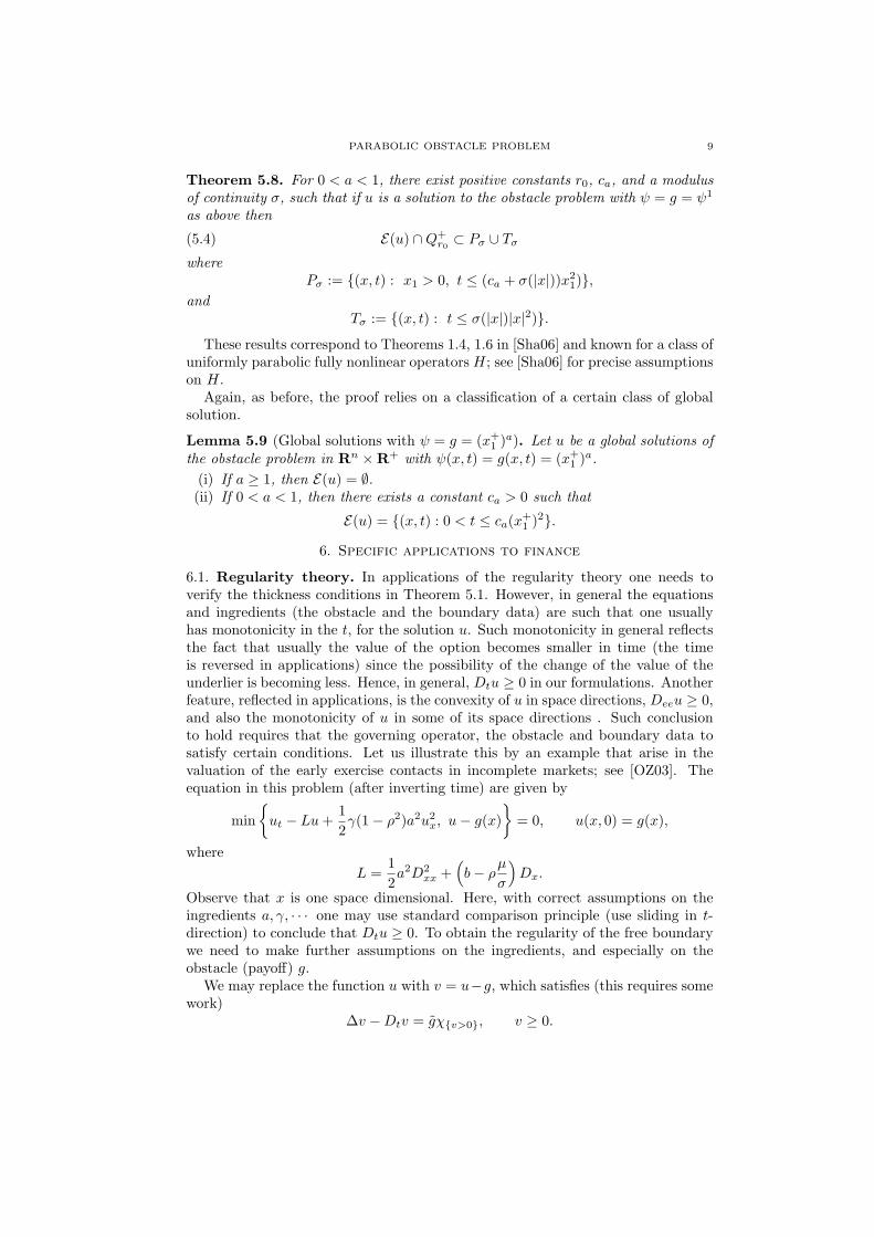
Below are presented pictures concerning the global solutions of the problem−∂tu+ ∆u ≤ 0, (−∂tu+ ∆u)(ψ − u) = 0,

u ≥ ψ(x), u(x, 0) = ψ(x)(A.1)

in R2 × (0, T ], where ψ(x) = min(x1, x2)+, and the two-dimensional Black-Scholesequation

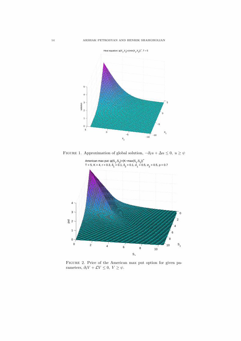
LV + ∂tV ≤ 0, (LV + ∂tV )(ψ − V ) = 0,

V ≥ ψ, V (S, T ) = ψ(S)(A.2)

in (R+)2 × [0, T ), where ψ(S) = min(E − S1)+, (E − S2)+. The equations aresolved numerically using finite difference schemes. For stability reasons we useimplicit methods as follows. Let A be the finite difference coefficient matrix anddenote the time index n. We then use Gaussian elimination to calculate un+1 fromun = Aun+1 for the forward equation and V n from V n+1 = AV n for the backwardsequation.

Since numerical computations can only be carried out in finite domains we ap-proximate R2 in (A.1) with [−10, 4] × [−10, 4] and (R+)2 in (A.2) by [0, 10.5] ×[0, 10.5]. We then impose as boundary conditions the solution to the correspondingone-dimensional problem on the boundaries where the obstacle is greater then orequal to zero, and zero boundary conditions on the boundaries where the obstacle iszero. The boundary conditions are verified to be reasonable by solving the problemin a larger domain and using the values of this solution as boundary conditions forthe smaller domain. The difference between the two approaches is insignificant.


−10

−5

0

5

−10−5

05

0

1

2

3

4

5

X1

Heat equation: ψ(X1,X

2)=(min(X

1,X

2))+, T = 5

X2

solu

tion

Figure 1. Approximation of global solution, −∂tu+ ∆u ≤ 0, u ≥ ψ

0

2

4

6

8

100 2 4 6 8 10

0

1

2

3

4

S1

S2

American max put: ψ(S1,S

2)=(K−max(S

1,S

2))+

T = 5, K = 4, r = 0.3, δ1 = 0.1, δ

2 = 0.1, σ

1 = 0.5, σ

2 = 0.5, ρ = 0.7

put

Figure 2. Price of the American max put option for given pa-rameters, ∂tV + LV ≤ 0, V ≥ ψ.


−3 −2 −1 0 1 2 3−2

0

2

0

1

2

3

4

5

X1

Free boundary for global solution for increasing time

X2

t

Figure 3. The contact set of the global solution for increasingtime. It exists on the diagonal x1 = x2.

−3 −2 −1 0 1 2 3 40

0.5

1

1.5

2

2.5

3

3.5

4

4.5

5

Free boundary on the diagonal x1=x

2 for increasing time

x1=x

2

t

Figure 4. The contact set on the diagonal x1 = x2 for the globalsolution. It decreases as time increases. The picture is similar forthe American max put on the diagonal.


01

23

45 0

12

34

5

0

1

2

3

4

5

S2

Free boundary for American max put for increasing time.

S1

T−

t

Figure 5. The exercise region (i.e. contact set) of the Americanmax put for increasing time.

0 0.5 1 1.5 2 2.5 3 3.5 4 4.5 50

0.5

1

1.5

2

2.5

3

3.5

4

4.5

5

Projection of exercise region in the S1,S

2−plane.

S1

S2

Figure 6. Projection of the exercise region of the American maxput at time 0. The payoff function (i.e. the obstacle) is zero outsidethe gray region.


References

[AUS03] D. E. Apushkinskaya, N. N. Ural′tseva, and H. Shahgolian, On the Lipschitz propertyof the free boundary in a parabolic problem with an obstacle, Algebra i Analiz 15(2003), no. 3, 78–103; translation in St. Petersburg Math. J. 15 (2004), no. 3, 375–391.MR MR2052937 (2005d:35276)

[BD97] Mark Broadie and Jerome Detemple, The valuation of American options on multipleassets, Math. Finance 7 (1997), no. 3, 241–286. MR MR1459060 (98b:90012)

[BDM05] A. Blanchet, J. Dolbeault, and R. Monneau, On the one-dimensional parabolic obsta-cle problem with variable coefficients, Elliptic and parabolic problems, Progr. Non-linear Differential Equations Appl., vol. 63, Birkhauser, Basel, 2005, pp. 59–66.MR MR2176699

[Caf77] Luis A. Caffarelli, The regularity of free boundaries in higher dimensions, Acta Math.139 (1977), no. 3-4, 155–184. MR MR0454350 (56 #12601)

[CC03] Xinfu Chen and John Chadam, Analytical and numerical approximations for the earlyexercise boundary for American put options, Dyn. Contin. Discrete Impuls. Syst. Ser.A Math. Anal. 10 (2003), no. 5, 649–660, Progress in partial differential equations(Pullman, WA, 2002). MR MR2013646 (2005k:91146)

[CPS04] Luis Caffarelli, Arshak Petrosyan, and Henrik Shahgholian, Regularity of a free bound-ary in parabolic potential theory, J. Amer. Math. Soc. 17 (2004), no. 4, 827–869 (elec-tronic). MR MR2083469 (2005g:35303)

[DFT03] Jerome Detemple, Shui Feng, and Weidong Tian, The valuation of American call op-tions on the minimum of two dividend-paying assets, Ann. Appl. Probab. 13 (2003),no. 3, 953–983. MR MR1994042 (2004e:91061)

[Fri75] Avner Friedman, Parabolic variational inequalities in one space dimension and smooth-ness of the free boundary, J. Functional Analysis 18 (1975), 151–176. MR MR0477461(57 #16988)

[LS01] Ki-Ahm Lee and Henrik Shahgholian, Regularity of a free boundary for viscosity solu-tions of nonlinear elliptic equations, Comm. Pure Appl. Math. 54 (2001), no. 1, 43–56.MR MR1787106 (2001h:35195)

[OZ03] A. Oberman and T. Zariphopoulou, Pricing early exercise contracts in incomplete mar-kets, Comput. Manag. Sci. 1 (2003), no. 1, 75–107.

[Sha06] Henrik Shahgholian, Free boundary regularity close to initial state for parabolic obstacleproblem, Trans. Amer. Math. Soc. (2006), to appear.

[vM74a] Pierre van Moerbeke, Optimal stopping and free boundary problems, Rocky MountainJ. Math. 4 (1974), 539–578. MR MR0381188 (52 #2085)

[vM74b] , An optimal stopping problem with linear reward, Acta Math. 132 (1974), 111–151. MR MR0376225 (51 #12405)

[Wan92a] Lihe Wang, On the regularity theory of fully nonlinear parabolic equations. I, Comm.Pure Appl. Math. 45 (1992), no. 1, 27–76. MR MR1135923 (92m:35126)

[Wan92b] , On the regularity theory of fully nonlinear parabolic equations. II, Comm. PureAppl. Math. 45 (1992), no. 2, 141–178. MR MR1139064 (92m:35127)

[Wan92c] , On the regularity theory of fully nonlinear parabolic equations. III, Comm.Pure Appl. Math. 45 (1992), no. 3, 255–262. MR MR1151267 (93c:35082)

Department of Mathematics, Purdue University, West Lafayette, IN 47907, USAE-mail address: [email protected]

Depatment of Mathematics, Royal Institute of Thechnology, 10044 Stockholm, Swe-den

E-mail address: [email protected]

parabolic obstacle problems applied to finance - department of

Documents