people.uncw.edupeople.uncw.edu/tagliarinig/courses/380/f2016 papers a… · web viewthe problem...

Chase ParkerFarris KhalidGabriel B. Gallagher

1Team Fast Gas

Abstract: Navigation is an important part of daily life. This report is about the design,

implementation, and analysis of Dijkstra’s, Johnson’s, and the Floyd-Warshall algorithms as they pertain to traveling from a given location on a grid in Wilmington, NC, to a final point which represents a gas station or convenience store where the user may fill up their vehicle or purchase necessary items. The algorithms were compared to Google Maps path selection for accuracy and efficiency.

IntroductionHuman error is the root cause of many inefficiencies. Such error may occur when an

individual forgets to fill up his/her gas tank on a very unpredictable day or an individual has no time to sit through traffic to get to one gas station that is only 0.2 miles away on South College at 5pm on a weekday.

Whether an individual has been a resident of Wilmington for many years or is new to the area, it is very hard to predict the shortest possible path on any given day because the shortest path doesn’t necessarily guarantee the fastest path. Speed is a measurement of time and distance. Our team aims to optimize time relative to distance by incorporating a unit of time as a form of distance.

Formal Problem Statement: When given a weighted network, which in this case will be a model of a given specified

area of the city of Wilmington, North Carolina, we want to analyze a specific set of points of interest, namely gas stations and convenience stores. The paths between each of these nodes will be given a value of E which corresponds to the expected time from entry to departure of the location.

Secondary nodes, which consist of intersections where the driver must stop and wait for traffic, will be given a value N, which, similar to the primary nodes, corresponds to the expected time from entry to departure of the location. Unlike the primary nodes, a driver cannot stop or complete the trip at a secondary node since a drive in real life would not end at an intersection (although some do, we are talking about Wilmington drivers, after all). A driver can, however, start from a secondary node. In fact, a driver will most often start from a secondary node and cannot start in between nodes, as it wouldn’t be practical for them to start them in the middle of a path and would require us to account for an almost infinite number of starting points.

Finally, each path must be weighted for traffic which will be adjusted based on the time of day to account for changes in traffic intensity along a specified route.


2When we put it all together, we have an equation such as:

“For all Routes, there exists a single route which is the shortest possible Route in terms of time.”

∀R ∃R0 = {ET + N} | 0 < R0 < Rn

This leads to the objective function, the goal of which is to minimize the cost of path P where:

Cost ( P )=∑i=1

n

d i∗w i

d i = distance between ith pairw i = traffic bias for ith pairn = number of vertices (intersections)

ContextThe problem of finding the shortest distance along a given path has been explored by

numerous parties. Google has been the most significant contributor to personal navigation since 2008, when it released the Google Maps mobile app. The Google Maps navigational system, to which we will be comparing our actual timings, uses a modified form of Dijkstra’s Algorithm for its most basic point-to-point navigational functionality. This will provide comparable results between our implementation of Dijkstra’s algorithm and a matured and tested implementation.

The Floyd-Warshall algorithm has been particularly successful in sparse graphs with long edges and few number of nodes and could prove to be very efficient for a subsection of Wilmington containing limited nodes and connected edges. However, this algorithm is much slower on denser, node-filled graphs, as the worst-case time complexity is O(n3) where n is the number of nodes.

Dijkstra’s algorithm, unlike Floyd-Warshall, is often more efficient at finding the shortest path between nodes on a denser graph, as one node is compared to all other nodes instead of producing an all-paths distance matrix. This will be used as a comparison relative to the performance of the Floyd-Warshall algorithm. Depending upon how dense the graph of nodes is, a combination of these two algorithms may prove beneficial.

The algorithms used to determine the shortest path, weighted by time, are established and well-studied. The efficiency of each algorithm is also known to be ideal under certain circumstances; therefore, a combination or modification of each algorithm may prove useful in certain scenarios.

The worst-case time complexity for Dijkstra’s algorithm is O(n2). The worst-case time complexity for Johnson’s algorithm is O(n2log(n) + n|E|) where E is the number of edges on the graph. This shows that Johnson’s algorithm should be slower than Dijkstra’s given a large set of


3nodes and their connecting edges. However, the primary purpose of Johnson’s algorithm is the ability to apply a matrix with negative edge values. This may become essential in a navigation algorithm, especially in the city of Wilmington, where roads often require a driver to make U-turns to travel to their destination. The worst-case space complexity for Floyd-Warshall’s algorithm is O(n2) with a worst-case time complexity of O(n3). Careful attention will be paid to this algorithm as it may prove to be the most efficient for our given graph size.

Dijkstra’s algorithm (Farris)All navigation problems require getting from a starting point to an ending point, often in

the shortest time or shortest distance possible. Such problems are referred to as minimum spanning distance problems. Dijkstra’s algorithm is a powerful and widely applicable tool for many minimum spanning problems. The algorithm has already been used to find directions between physical locations by apps such as Mapquest and Google Maps. For our purposes, we know that Dijkstra’s algorithm is designed to use a single weight, usually either time or distance, but not both. We will need to modify our final Algorithm to account for both variables. Dijkstra’s algorithm also specifically finds the minimum spanning distance. However, when one modifies the algorithm to consider two weights, one must also consider that the shortest path in terms of time from point A to point B may not always be the shortest path in terms of distance, and vice versa. Our algorithm will ultimately need to take several routes in terms of time, and then weigh each for distance to find the most efficient route of the set. This is something that Dijkstra’s algorithm, in its simplest form, is not designed to do.


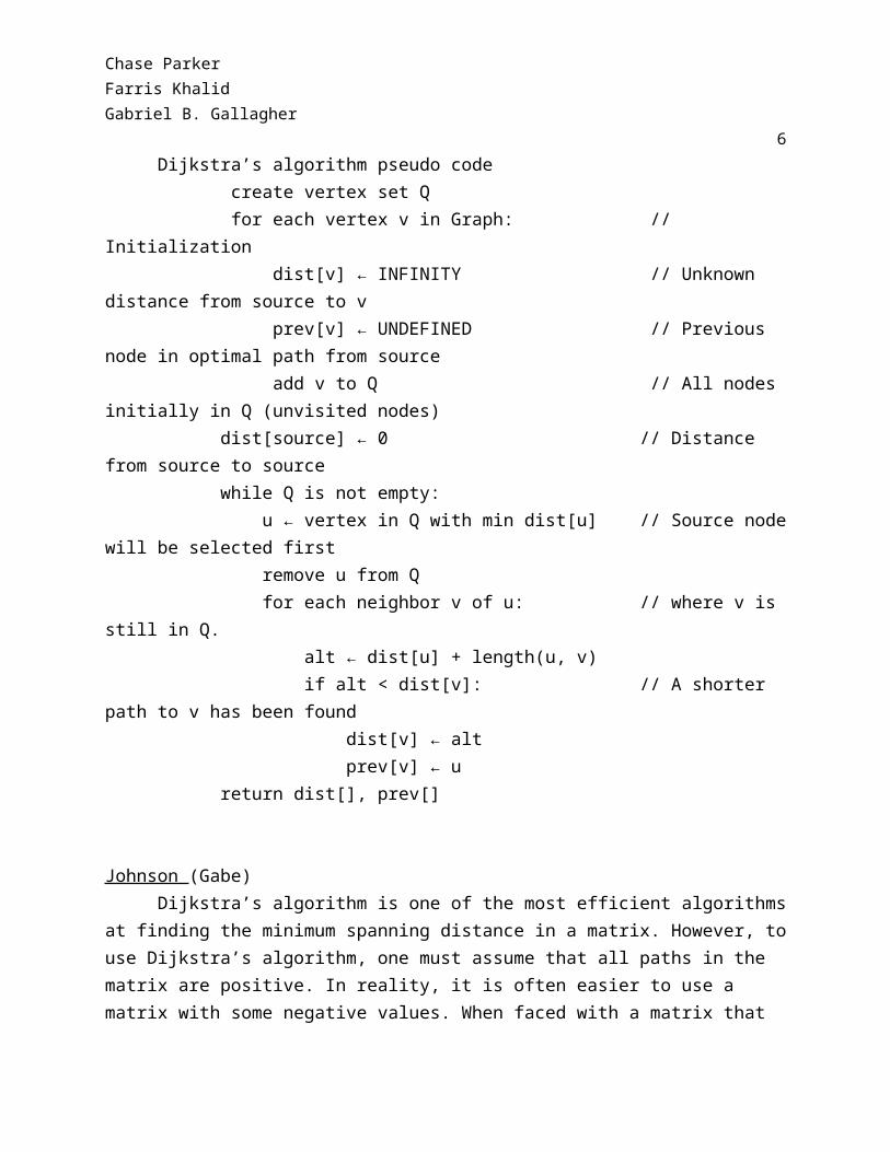
4Dijkstra’s algorithm pseudo code create vertex set Q for each vertex v in Graph: // Initialization dist[v] ← INFINITY // Unknown distance from source to v prev[v] ← UNDEFINED // Previous node in optimal path from source add v to Q // All nodes initially in Q (unvisited nodes) dist[source] ← 0 // Distance from source to source while Q is not empty: u ← vertex in Q with min dist[u] // Source node will be selected first remove u from Q for each neighbor v of u: // where v is still in Q. alt ← dist[u] + length(u, v) if alt < dist[v]: // A shorter path to v has been found dist[v] ← alt prev[v] ← u return dist[], prev[]

Johnson (Gabe)Dijkstra’s algorithm is one of the most efficient algorithms at finding the minimum

spanning distance in a matrix. However, to use Dijkstra’s algorithm, one must assume that all paths in the matrix are positive. In reality, it is often easier to use a matrix with some negative values. When faced with a matrix that contains negative paths, Dijkstra’s algorithm doesn’t simply lose efficiency, it breaks and becomes useless. Johnson’s algorithm attempts to circumvent this obvious weakness by first using the Bellman-Ford algorithm, which reweights the paths in the original matrix. It does this by iterating over the matrix and adjusting the values such that each path is adjusted to a positive value, while retaining its original distance relative to every other path in the matrix. For example, if a matrix contained two paths, one with a value of 2 and another with a value of -1, the path with a value would become 1, while the path with a value of 2 would become 4. Finally, Dijkstra’s algorithm is used to find the minimum spanning distance in the newly weighted matrix. Johnson’s algorithm is an important example in our project because it successfully incorporates information from two different weight variables to find an efficient spanning distance.

The complexity of Johnson’s algorithm depends on the implementation of Dijkstra’s algorithm. In this experiment, we used an implementation of Dijkstra’s which had a worst-case scenario of O(n2). Therefore, our implementation of Johnson’s had a worst-case scenario of O(n3logn).


5

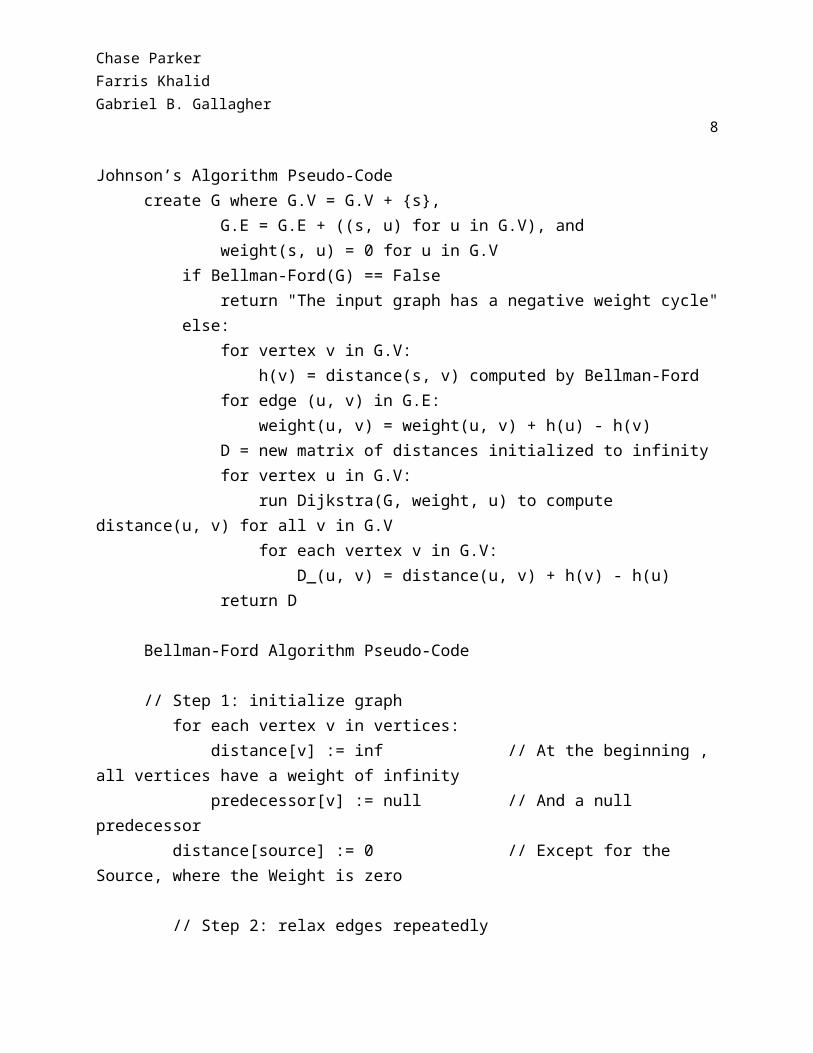
Johnson’s Algorithm Pseudo-Codecreate G where G.V = G.V + {s}, G.E = G.E + ((s, u) for u in G.V), and weight(s, u) = 0 for u in G.V if Bellman-Ford(G) == False return "The input graph has a negative weight cycle" else: for vertex v in G.V: h(v) = distance(s, v) computed by Bellman-Ford for edge (u, v) in G.E: weight(u, v) = weight(u, v) + h(u) - h(v) D = new matrix of distances initialized to infinity for vertex u in G.V: run Dijkstra(G, weight, u) to compute distance(u, v) for all v in G.V for each vertex v in G.V: D_(u, v) = distance(u, v) + h(v) - h(u) return D

Bellman-Ford Algorithm Pseudo-Code

// Step 1: initialize graph for each vertex v in vertices: distance[v] := inf // At the beginning , all vertices have a weight of infinity predecessor[v] := null // And a null predecessor distance[source] := 0 // Except for the Source, where the Weight is zero

// Step 2: relax edges repeatedly for i from 1 to size(vertices)-1: for each edge (u, v) with weight w in edges: if distance[u] + w < distance[v]: distance[v] := distance[u] + w predecessor[v] := u

// Step 3: check for negative-weight cycles for each edge (u, v) with weight w in edges: if distance[u] + w < distance[v]: error "Graph contains a negative-weight cycle" return distance[], predecessor[]


6

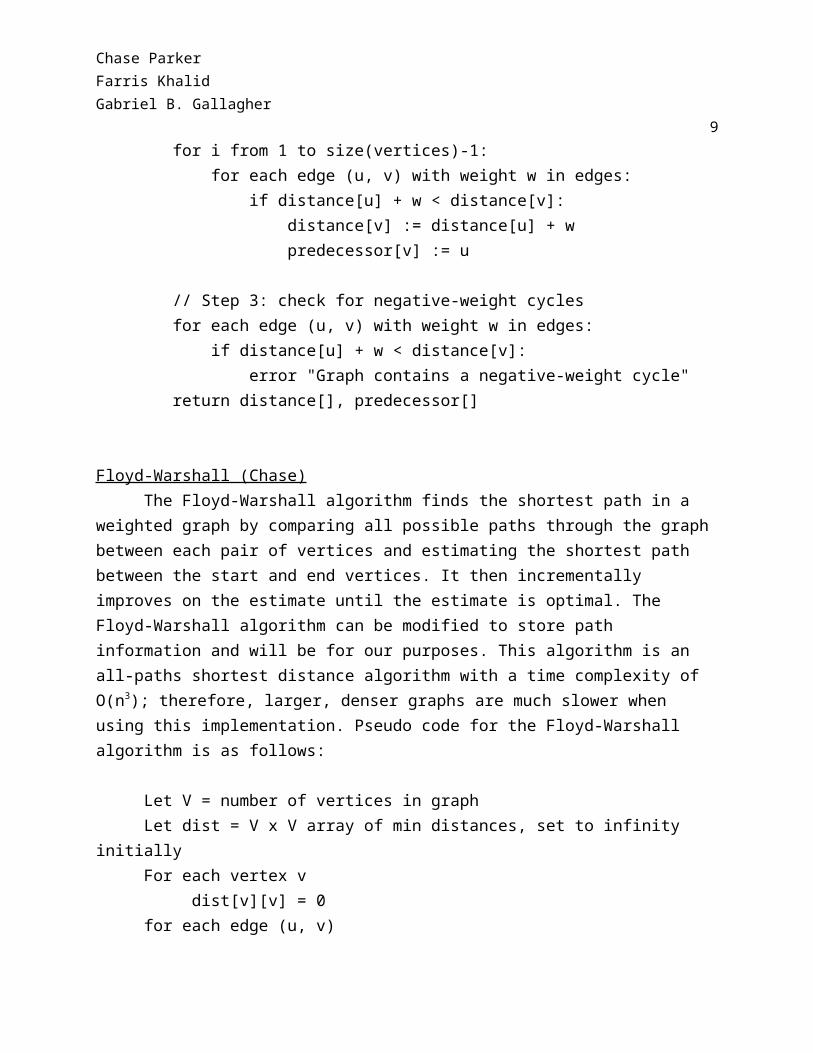
Floyd-Warshall (Chase)The Floyd-Warshall algorithm finds the shortest path in a weighted graph by comparing

all possible paths through the graph between each pair of vertices and estimating the shortest path between the start and end vertices. It then incrementally improves on the estimate until the estimate is optimal. The Floyd-Warshall algorithm can be modified to store path information and will be for our purposes. This algorithm is an all-paths shortest distance algorithm with a time complexity of O(n3); therefore, larger, denser graphs are much slower when using this implementation. Pseudo code for the Floyd-Warshall algorithm is as follows:

Let V = number of vertices in graphLet dist = V x V array of min distances, set to infinity initiallyFor each vertex v

dist[v][v] = 0for each edge (u, v)

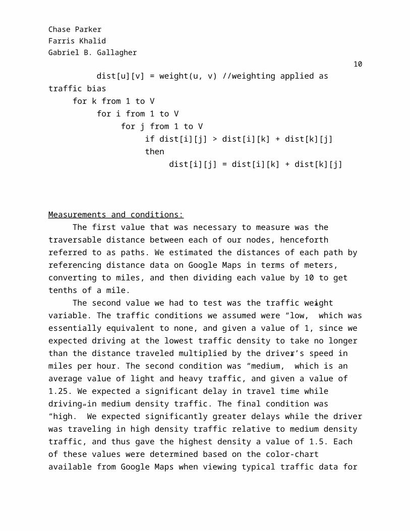
dist[u][v] = weight(u, v) //weighting applied as traffic biasfor k from 1 to V

for i from 1 to Vfor j from 1 to V

if dist[i][j] > dist[i][k] + dist[k][j]then

dist[i][j] = dist[i][k] + dist[k][j]

Measurements and conditions:The first value that was necessary to measure was the traversable distance between each

of our nodes, henceforth referred to as paths. We estimated the distances of each path by referencing distance data on Google Maps in terms of meters, converting to miles, and then dividing each value by 10 to get tenths of a mile.

The second value we had to test was the traffic weight variable. The traffic conditions we assumed were “low,” which was essentially equivalent to none, and given a value of 1, since we expected driving at the lowest traffic density to take no longer than the distance traveled multiplied by the driver’s speed in miles per hour. The second condition was “medium,” which is an average value of light and heavy traffic, and given a value of 1.25. We expected a significant delay in travel time while driving in medium density traffic. The final condition was “high.” We expected significantly greater delays while the driver was traveling in high density traffic relative to medium density traffic, and thus gave the highest density a value of 1.5. Each of these values


7were determined based on the color-chart available from Google Maps when viewing typical traffic data for a given time and day. Hourly traffic conditions were recorded for each edge in the graph from 12pm to 5pm on a given day and averaged to obtain our traffic bias for that day during the 12-5pm time block. Our timed driving measurements were all taken during this time.

Each traffic condition is given a value that will increase the relative distance to a perceived distance. In the end result, we would like the perceived distance to outperform the relative distance since time will be a major factor in computation of the fastest route. By applying this traffic bias, we also hope to simulate additional time spent in traffic, a variable not considered by any of our original algorithms.

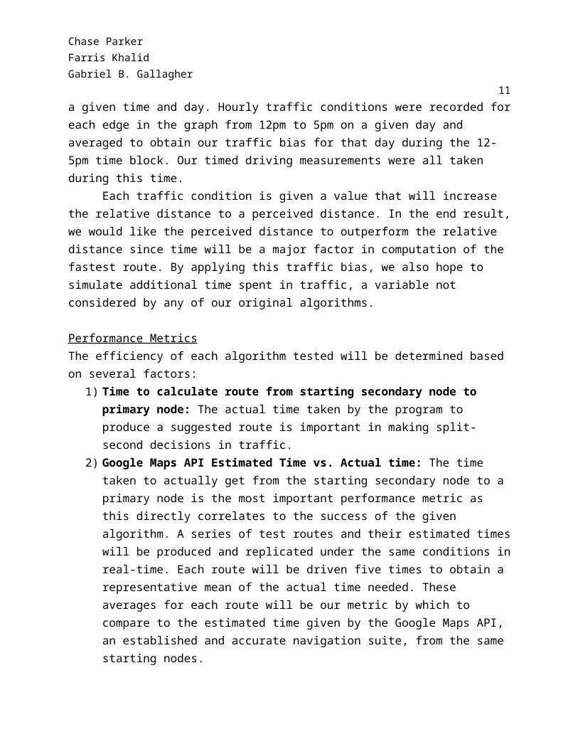
Performance MetricsThe efficiency of each algorithm tested will be determined based on several factors:

1) Time to calculate route from starting secondary node to primary node: The actual time taken by the program to produce a suggested route is important in making split-second decisions in traffic.

2) Google Maps API Estimated Time vs. Actual time: The time taken to actually get from the starting secondary node to a primary node is the most important performance metric as this directly correlates to the success of the given algorithm. A series of test routes and their estimated times will be produced and replicated under the same conditions in real-time. Each route will be driven five times to obtain a representative mean of the actual time needed. These averages for each route will be our metric by which to compare to the estimated time given by the Google Maps API, an established and accurate navigation suite, from the same starting nodes.

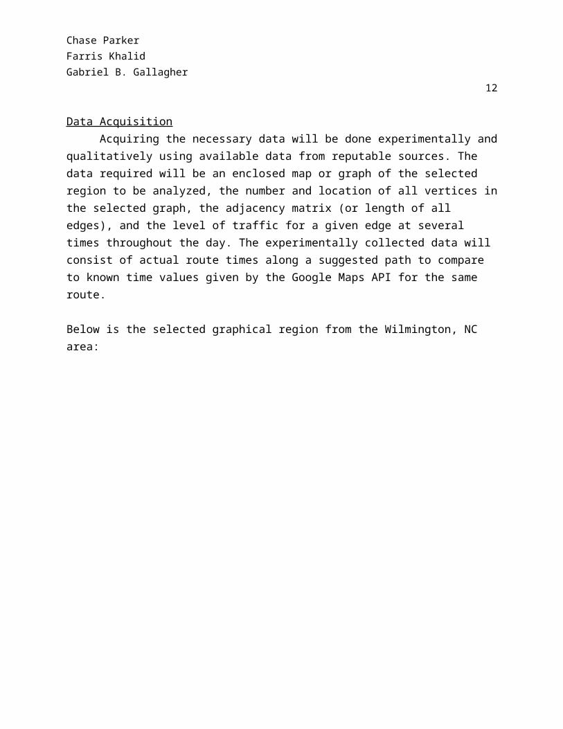
Data AcquisitionAcquiring the necessary data will be done experimentally and qualitatively using

available data from reputable sources. The data required will be an enclosed map or graph of the selected region to be analyzed, the number and location of all vertices in the selected graph, the adjacency matrix (or length of all edges), and the level of traffic for a given edge at several times throughout the day. The experimentally collected data will consist of actual route times along a suggested path to compare to known time values given by the Google Maps API for the same route.

Below is the selected graphical region from the Wilmington, NC area:


8

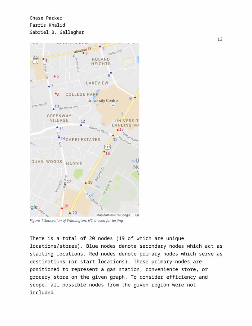
Figure 1 Subsection of Wilmington, NC chosen for testing

There is a total of 20 nodes (19 of which are unique locations/stores). Blue nodes denote secondary nodes which act as starting locations. Red nodes denote primary nodes which serve as destinations (or start locations). These primary nodes are positioned to represent a gas station, convenience store, or grocery store on the given graph. To consider efficiency and scope, all possible nodes from the given region were not included.

The following adjacency matrix results from the set of nodes shown above. Note that the edge lengths in the adjacency matrix are in units of 1/10th of a mile and were determined based on the distance between nodes as given by the Google Maps API.


9

Adjacency Matrix (in tenths of a mile)

Table 1 Adjacency Matrix used for all algorithms (obtained from Google Maps)

1 2 3 4 5 6 7 8 9 10 11 12 13 14 15 16 17 18 19 201 0 3.5 0 0 2.9 0 3.1 0 0 0 0 0 0 0 0 0 0 0 0 02 3.5 0 .9 2.8 0 0 0 0 0 0 0 0 0 0 0 0 0 0 0 03 0 .9 0 1.9 0 0 0 0 0 0 0 0 0 0 0 0 0 0 0 04 0 2.8 1.9 0 0 3 0 0 0 0 0 0 0 0 0 0 0 0 0 05 2.9 0 0 0 0 0 1.5 0 0 0 0 0 0 0 0 0 0 0 0 06 0 0 0 3 0 0 0 0 3.8 0 0 0 0 0 0 0 0 0 0 07 3.1 0 0 0 1.5 0 0 .1 0 2.5 0 0 0 0 0 0 0 0 0 08 0 0 0 0 0 0 .1 0 0 1.8 0 0 0 0 0 0 0 0 0 09 0 0 0 0 0 3.8 0 0 0 0 0 0 4.1 0 0 0 0 0 0 0

10 0 0 0 0 0 0 2.5 1.8 0 0 1.9 0 0 0 0 0 0 0 0 011 0 0 0 0 0 0 0 0 0 1.9 0 2.5 0 1.1 0 0 0 0 0 012 0 0 0 0 0 0 0 0 0 0 2.5 0 0 0 1.9 0 0 0 0 013 0 0 0 0 0 0 0 0 4.1 0 0 0 0 0 .7 0 0 0 0 014 0 0 0 0 0 0 0 0 0 0 1.1 0 0 0 0 0 5.2 0 0 015 0 0 0 0 0 0 0 0 0 0 0 1.9 .7 0 0 1.7 0 0 0 016 0 0 0 0 0 0 0 0 0 0 0 0 0 0 1.7 0 0 4.2 0 017 0 0 0 0 0 0 0 0 0 0 0 0 0 5.2 0 0 0 .7 2.7 018 0 0 0 0 0 0 0 0 0 0 0 0 0 0 0 4.2 .7 0 0 3.719 0 0 0 0 0 0 0 0 0 0 0 0 0 0 0 0 2.7 0 0 120 0 0 0 0 0 0 0 0 0 0 0 0 0 0 0 0 0 3.7 1 0

ResultsTable 2 Results of our algorithms produced path vs. Google Produced path


10

Figure 2 Route times for various algorithms and start/end node pairs (red=different path from Google)

Figure 3 Same data as Figure 2 above, represented as a percentage of our Average route time divided by Google's Estimated time


11Analysis

From the start of the implementation of our algorithms in a real-world setting, it became clear that Johnson’s algorithm would not be useful for the scope of our project. The idea behind Johnson’s algorithm is to allow for implementation of a matrix with negative distances. We thought that this would be the case in situations where the driver would have to make a U-turn in route to their destination, which is often necessary while driving in Wilmington. However, our implementation did not pass any negative weights to Dijkstra’s algorithm, making the Dijkstra’s algorithm more efficient than Johnson’s in all scenarios.

Dijkstra’s algorithm was the fastest with a runtime of 15 milliseconds, which was the expected result as it had the lowest time complexity. Floyd-Warshall had a runtime of 32 milliseconds, which was faster than expected, given the average complexity of O(n3), but still slower than Dijkstra’s. This was most likely due to the Dijkstra’s code not being completely optimized for placement of timers in Java.

The most striking difference between our results and those of Google Maps was on the route from node 6 to node 8. To reduce the scope of our experiment and make it more manageable, we removed several back-road routes simply to reduce the number of possible paths for real world testing. This resulted in us never including a path between node 6 and node 12 which was the path Google selected to go from node 6 to node 8. Our algorithm ultimately selected 6 4 2 1 7 8, which was the optimal path given the information in our matrix. Google selected 6 12 11 10 8, which is most likely the real world optimal path prior to accounting for traffic weights.

This difference in path selection shows that our implementation of the Floyd-Warshall algorithm chose a route different from the one chosen by Google Maps, yet our average route time tested for our produced route was within 3 seconds of the estimated Google Maps time for an alternate route. This shows that there is some merit to the method chosen to scale the distance by a traffic bias multiplier. Future work will included more nodes and possible paths for testing to further validate the scaling of distance according to available and relevant traffic data.

Existing HolesOne of the major holes in our experiment is the obvious simplicity in our traffic weights.

If we were to expand the scope of our project, we would have figured out a way to get much more in depth traffic data to make our time estimates more accurate.

Another hole in our experiment was the lack of a calculation for stopping at the nodes. The nodes in our experiment represent real world traffic stops, such as traffic light, stop signs, and intersections. The driver must stop at these locations, and it will take longer to move through these stops as the amount of traffic increases. This would have required an altered implementation of our algorithms which would have accounted for time variables on each of our nodes. This type of implementation would have required a much more complex matrix, and more


12complex algorithms to account for it. This was outside the scope of our project, and why we didn’t include it in this experiment.

The final hole we will discuss was our implementation of Dijkstra’s algorithm. When using a priority queue, Dikstra’s algorithm has a worst-case performance figure of O(nlogn), which is far superior to the matrix implementation used in this experiment, which has a worst-case performance of O(n2). Matrix data is far easier to work with in this project due to the ease of visualizing a map of Wilmington in terms of a matrix. However, if we had the time to build a priority queue containing all of the relative path values for the scope of our map, it would provide a much more efficient implementation of Dijkstra’s algorithm. However, the end results would have been the same in terms of which paths were chosen by the algorithm, so this will be a more important consideration when we expand the map to include more paths, which will yield a more noticeable run-time difference between a O(n2) worst case performance and O(nlogn).

Interpretation and ConclusionsAll of the routes suggested by our algorithms were identical to those chosen by Google,

except for one. This suggests that our algorithms closely emulate those used by Google for geographical mapping and are on par with the ones used in real world optimal direction calculation applications. We believe that we are on the right track with our chosen algorithms, as well as our implementation of those algorithms.

Future WorkOne of the major additions we would make to this project would be an app that allows

more user input and variability. The current version of our algorithms read values from a .CSV file which cannot be updated directly from our program. This means that the algorithms only work in our specified region of Wilmington, using our specified nodes.

Of course, if we wanted to build an app, we would have to substantially increase the dimensions of our map. For simplicity, our map only includes a small segment of the town to the immediate west of the UNC Wilmington campus. We would like to first expand it to all of Wilmington and possibly neighboring cities in the future.

Incorporating GPS would useful functionality to implement alongside our algorithms. This would allow real time traffic analysis as well as the ability for users to be immediately placed on the matrix.


13Bibliography

Sedgewick, R., & Wayne, K. Shortest Paths. Retrieved September 29, 2016, from Princeton University, https://www.cs.princeton.edu/~rs/AlgsDS07/15ShortestPaths.pdf

Alsedà, L. Dijkstra’s Shortest Path Algorithm. Retrieved September 29, 2016, from Universitat Autonoma De Barcelona, http://mat.uab.cat/~alseda/MasterOpt/MyL09.pdf

Tseng, W.-L. Graph Theory. Retrieved September 29, 2016, from Cornell University, http://www.cs.cornell.edu/~wdtseng/icpc/notes/graph_part3.pdf

Getting started. (2016, September 25). Retrieved September 29, 2016, from Google Maps API, https://developers.google.com/maps/documentation/directions/start

Floyd-Warshall algorithm. Retrieved September 29, 2016, from George Mason University, http://masc.cs.gmu.edu/wiki/FloydWarshall

Aini, A., & Salehipour, A. (2012). Speeding up the Floyd–Warshall algorithm for the cycled shortest path problem. Applied Mathematics Letters, 25(1), 1–5. doi:10.1016/j.aml.2011.06.008

Levitin, A. (2007). Introduction to the design & analysis of algorithms (3rd ed.). Boston: Pearson Addison-Wesley.

http://masc.cs.gmu.edu/wiki/FloydWarshall

https://developers.google.com/maps/documentation/directions/start

http://www.cs.cornell.edu/~wdtseng/icpc/notes/graph_part3.pdf

http://mat.uab.cat/~alseda/MasterOpt/MyL09.pdf

https://www.cs.princeton.edu/~rs/AlgsDS07/15ShortestPaths.pdf

people.uncw.edupeople.uncw.edu/tagliarinig/courses/380/f2016 papers a… · web viewthe problem...

Documents