service woes at speedy delivery: finding the … woes at speedy delivery: finding the shortest route...

Service Woes at Speedy Delivery: Finding the Shortest Route

Teacher Resources

Operations Research: A Brief History The field of Operations Research (OR) has its roots in the years just prior to World War II as the British prepared for the anticipated air war. In 1937, field tests started on what was later to be called radar. In 1938, experiments began to explore how the information provided by radar should be used to direct deployment and use of fighter planes. Until this time, the word experiment conjured up the picture of a scientist carrying out a controlled investigation in a laboratory. In contrast, the multi-disciplinary team of scientists working on this radar-fighter plane project studied the actual operating conditions of these new devices and designed experiments in the field of operations and the new term operations research was born. The team’s goal was to derive an understanding of the operations of the complete system of equipment, people, and environmental conditions (e.g. weather, nighttime) and then improve upon it. Their work was an important factor in winning the Battle of Britain and operational research eventually spread to all of the military services. Several of the leaders of this effort were Nobel laureates in their original fields of study. Their approach was later paralleled in the US, with the first team working on anti-submarine tactics. The US group developed a series of mathematical models entitled search theory that was used to develop optimal patterns of air search. Like their British counterparts, they got close to the action by riding in airplanes on patrol just as the modern operations researcher might ride in a police car or spend time in an automotive assembly plant. Currently, every branch of the military has its own operations research group that includes both military and civilian personnel. They play a key role in both long-term strategy and weapons development, as well as directing the logistics of actions such as Operation Desert Storm. In addition, the National Security Agency has its own Center for Operations Research. OR moved into the industrial domain in the early fifties and paralleled the growth of computers as a business planning and management tool. As the field evolved, the core moved away from interdisciplinary teams to a focus on the development of mathematical models that can be used to model, improve, and even optimize real-world systems. These mathematical models include both deterministic models such as mathematical programming, routing, or network flows and probabilistic models such as queuing, simulation and decision trees. These mathematical modeling techniques form the core curriculum in masters degree and doctoral programs in operations research which can be found in either engineering or business schools. Most mathematics departments also offer one or more introductory operations research courses at the junior or senior undergraduate level.

Service Woes at Speedy Delivery: Teacher Resources

2

Routing Through Networks: Background

Graphs and networks are collections of nodes and arcs. The nodes are used to represent cities, major intersections, or individual customer locations. The arcs are used to represent the linkages between nodes. The linkages could be telecommunication lines or roads. The links can be one-way or bi-directional. Numeric values on the links can represent the actual length of the link, the distance as the crow flies, or the time to traverse the link. In routing applications, it is important to use travel times and not just distances. Two miles on the open road are traversed much faster than two miles through city streets. In addition, these data will often need to be adjusted by time of day. The field of graph theory dates back more than two hundreds years with mathematicians such as Euler actively involved in its theoretical analysis. Graph theorists were primarily interested in understanding the properties of different graph structures without numeric values attached to the arcs. With the growth of computers, the study of networks moved into a new phase in the 1950s and 60s that focused on the development of efficient algorithms to solve optimization problems in routing. Networks were no longer just a collection of nodes and arcs; arcs now included numeric values which could represent either distance or time. One of the first class of problems that was solved related to finding the shortest path between two points (nodes) on a network. A computer scientist named Dijkstra developed one of the first efficient algorithms for solving this problem. Dijkstra’s algorithm is the basis for widely available software that responds to requests for finding the shortest or fastest route to a specific location. In addition, this algorithm is an important element of the management of information traveling through a telecommunications network. In the 1970s operations researchers began to study two classes of vehicle routing problems, the traveling salesman problem and the Chinese postman problem. One class of problems involves an individual or vehicle traveling along the shortest route from node to node, visiting every node in the network and then returning home to its base. (The 19th century mathematician William Hamilton first posed the question of the existence of a circuit that visited each node once and only once.) This problem is called the traveling salesman problem (TSP), as it represents the challenge facing a salesman who must travel from city to city and return home. It is part of a broad class of problems for which we know it is NOT possible to develop algorithms that are guaranteed to find the absolute optimal solution in a reasonable period of time. Instead, operations researchers work on developing heuristic algorithms that search for good or near optimal solutions. These algorithms generally have two phases. The first phase attempts to find a good initial solution. The second phase involves minor modifications to the best solution found so far in order to create better and better routes. In practical applications, the transportation manager rarely deals with routing just one vehicle. Instead, he has a whole fleet of vehicles. In this case the algorithms must divide the set of nodes (pick-up or delivery points) into separate routes, with each route assigned to a vehicle. Companies such as Federal Express have large internal operations research groups working on a wide range of issues related to the routing of vehicles and the


3

overall management of the truck fleet. In contrast, a bank such as Wells Fargo or Bank of America might commission a consulting firm to design the routes for a fleet of trucks. These trucks pick up cancelled checks several times a day at the bank branch offices and then deliver them to a check clearing house for posting with the Federal Reserve for collection of funds. School bus routing also involves applying algorithms used to solve TSP.

In the not so good old days, routing software ran in batch mode on a mainframe computer. The solution was printed out as a sequential list of stops. To see the route, an individual would take a piece of see-through vellum, lay it over a big map and trace the route by hand. If a mistake had been made in the input data or new stops had to be added, the process would have to start all over again and the original piece of vellum tossed out. In the 1980s, the personal computer revolutionized this process. Not only could the algorithms be run almost instantaneously on the manager’s desk, more importantly the solutions could be linked to widely available geographic information systems (GIS). As a result the routes could be shown on the computer screen overlaid on the actual street network. This new capability motivated a change in the design of routing packages to enable the experienced manager to contribute to the design and modification of the final routes. No mathematical model can capture all aspects of a complex problem. Thus, the need to tweak a solution to account for something not explicitly included in the model is not uncommon. PC based systems have enabled managers to easily adjust the final routes.

The Chinese Postman Problem (CPP) is a close cousin to TSP. In this routing problem the traveler must traverse every arc (i.e. road link) in the network. The name comes from the fact that a Chinese mathematician, Mei-Ko Kwan (1962), developed the first algorithm to solve this problem for a rural postman. It is an extension to one of the earliest graph theory questions, the Königsberg Bridge Problem, which was studied by Euler (1736). The Pregel River runs through the city of Königsberg in Germany. In a city park seven bridges cross branches of the river and connect two islands with each other and with opposite banks of the river. For many years the citizens of Königsberg tried to take walks that took them over each bridge once without retracing any part of their path. Euler was able to prove that such a walk is impossible. In general, graph theorists are interested in understanding whether or not a circuit exists that does not require traversing the same arc twice. Operations researchers are interested in finding the shortest route in any type of network. The Chinese Postman class of problems is relevant to a number of other services. Garbage collection, street sweeping, salting or gritting of icy roads, and snow plowing are some of the other services for which vehicle routing algorithms have been applied. Meter readers also must travel up and down every street. Checking roads for potholes or serious deterioration or checking pipelines for weak spots also fall into this class of problems. In the ever complex real-world additional constraints can arise that complicate the search for efficient routes. Labor contracts may require that the routes of different drivers must be approximately of equal length. There may be significant time restrictions or time


4

windows on when a vehicle must visit a specific location to make a delivery or pick-up. The vehicle making pick-ups may also have capacity limitations such as a garbage truck which would restrict the maximum length of a route. Uncertainty can also complicate route planning. Trucks that deliver gasoline or oil, can’t be sure when they set out as to how much they will have to pump into each of the tanks on their route. Planning routes is just one piece of the decision making puzzle that a transportation manager must put together. The manager must also make decisions as to the size of the fleet, the location of depots or landfills, the size and type of vehicles. There are dozens of commercial software packages to aid in routing and scheduling vehicles. A generic website that can lead the reader to many packages for solving such problems can be found at http://www.transportweb.com/software.html. Examples of specific software packages can be found at: http://www.optrak.co.uk/ and http://www.navesinklogistics.com/routing.html. Reference:

Bodin, Lawrence D., “Twenty Years of Routing and Scheduling,” Operations Research, Vol. 38, #4, pp. 571-579, 1990.

Teaching Notes Objectives of the Module In this module, students will become familiar with the basic elements of a network. They will learn the meanings of nodes, arcs, and weights (distances, travel times, costs) associated with arcs, while developing their mathematical reasoning skills. Students will learn to use an algorithm to systematically find the optimal solution to a problem. In routing applications, the optimal solution typically minimizes distance, time, or cost. Several case studies are included in these resources, so that students can learn about the various ways government and industry solve large-scale versions of the problems presented in the module. The case studies are also given so that students become aware that many well-known companies use operations research daily. Using the Module The purpose of this module is to show students a method (algorithm) for finding the shortest route in a network. The network is comprised of arcs (segments) and nodes (vertices). A path is a sequence of connected arcs joining two nodes in the network. In our sample problem, the nodes are business locations and the arcs are streets that connect them. The goal is to traverse the network from one location to another, finding the path requiring the shortest time. While students may determine the shortest time through a “guess and check” process, the algorithm developed in this module, Dijkstra’s Algorithm, is a systematic method of finding the shortest path.


5

The sample problem poses the question of determining the shortest path from node A to node E. Initially, students are asked some questions related to the figure. The numbers associated to the individual arcs refer to the average time it takes to travel along that arc, going from one node to another. Students are asked to find the shortest path on their own. While some students may end up finding the correct path, most probably will not. Students should be given time to arrive at their answers, as well as time to check their answers with others nearby, but you may want to encourage them to find just “a short route” in order to expedite things. The Shortest Path Algorithm explains the process used in the module for determining the shortest route in the sample problem. The algorithm is outlined in detail on page 2 of the student activity. This algorithm has the property of generating not only the shortest path from node A to node E, but also the shortest path from node A to other nodes in the network. The algorithm can be extended to find the shortest path to every other node with little additional effort. You may want to point out to students that although each node (except the starting point) first appears in the table as an uncircled adjacent node, each node on the shortest path will eventually also appear as a circled node. Conversely, some circled nodes will not end up on the shortest path. Some students may want to shade instead of circle the nodes in the network. You may want to go through the chart on page 2 with the students, one step at a time, so that they get a clear understanding of the algorithm. Some students may have difficulty with step 6 of the algorithm. For example, starting at node A, one should first choose path AB, because this path is shorter than AF; hence, node B becomes the next circled node. It may then occur to some students that BF is the shortest path. However, all of the paths must originate at node A, the original starting point. Therefore, BF is just a portion of path ABF, with a total length of 7 > 5 = AF. Therefore, path AF should be the selection. Node F becomes the next circled node. Since both paths ABF and AF end at the same node, you only want the path that is the shortest. Therefore, path ABF would never be taken in the network. We indicate this in the drawing by striking out arc BF. In question 20, students are asked if, when the driver needs to travel from node E back to node A, he should use the same path in reverse. While this may seem an obvious answer, it would be necessary to use the algorithm again if some arcs cannot be used on the way back (i.e. one-way streets). One of the extensions deals with the problem of one-way streets in the network. In question 21, students need to find the shortest path from node E to node B. This requires using the algorithm with a new table. All paths will start at node E, with node E being the first circled node. You may want to point out that the base example developed in the student activity does not have a unique solution. This is due to the arbitrary resolution of ties. See answer 17 in the solution set.


6

Extensions Four extensions are provided in the packet. The first extension is a more difficult version of the sample problem, because the network contains more nodes and arcs. The second requires the construction of a table of distances (similar to tables found on maps or in atlases) from the graph in the Extension 1. The third extension asks students to construct a weighted network from a table of distances. Finally, the fourth further complicates the Extension 1 by adding one-way streets to that network. Extension 4 contains one-way streets. This aspect of the problem is captured through the concept of adjacent nodes. For example, if you are at node J in this network, node K is not an adjacent node due to the one-way arc from node K to J. In extension 4, students can find the required shortest route without finding the shortest route to each of the other nodes. With a little extra effort, the algorithm can be continued to generate the shortest path to every other node in the network.


7

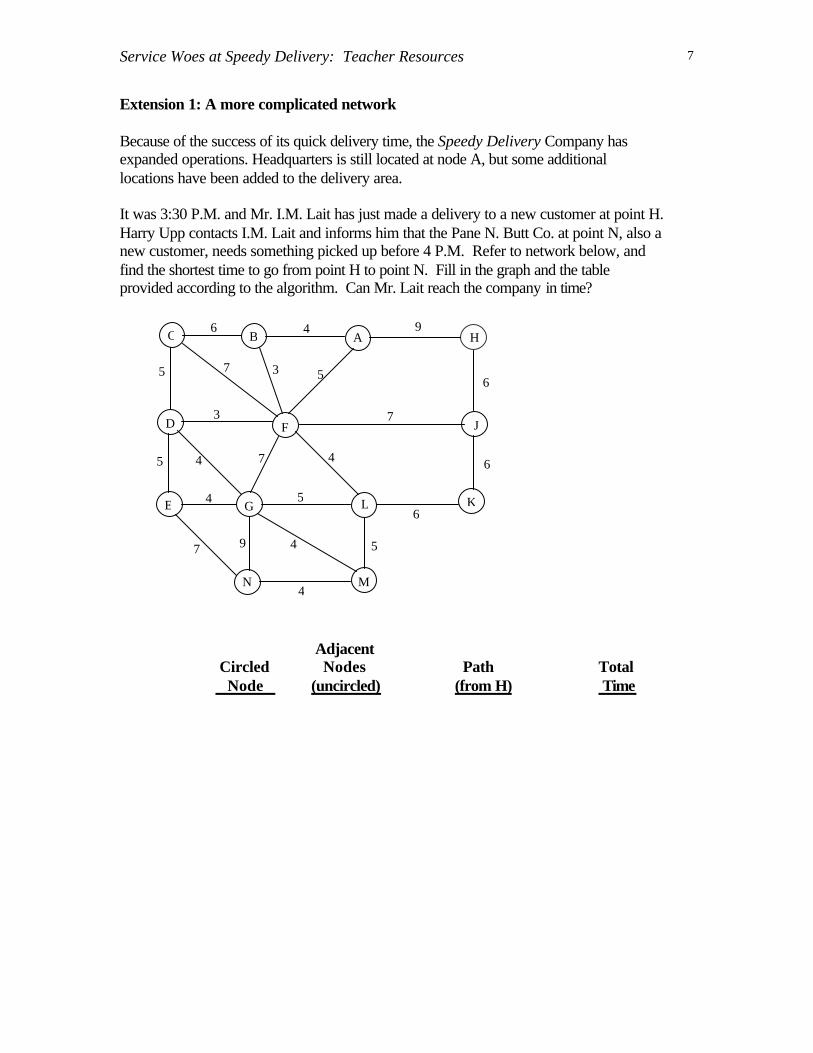
Extension 1: A more complicated network Because of the success of its quick delivery time, the Speedy Delivery Company has expanded operations. Headquarters is still located at node A, but some additional locations have been added to the delivery area. It was 3:30 P.M. and Mr. I.M. Lait has just made a delivery to a new customer at point H. Harry Upp contacts I.M. Lait and informs him that the Pane N. Butt Co. at point N, also a new customer, needs something picked up before 4 P.M. Refer to network below, and find the shortest time to go from point H to point N. Fill in the graph and the table provided according to the algorithm. Can Mr. Lait reach the company in time?

Adjacent Circled Nodes Path Total Node (uncircled) (from H) Time

J

C B A H

D F

E G L K

N M 4

7 9 4 5

5 6

6

6

9

7

4 6

5

5

7

3

3 5

4

4

7 4


8

Extension 2: The Other Way Around Perhaps you have seen a table showing the travel times between major cites on a map. Using the weighted network from figure 2 in the Speedy Delivery problem, make such a table. Be sure to show the travel times between every pair of nodes in the network. A B C D E F G

A --- 13 B --- C --- D --- E 13 --- F --- G ---

7

7

4

4 5

5 3

5 3

4 6 C B A

D

E

F

G


9

Extension 3: Cities in Michigan Helen Wheels drives a truck "over the road" between the cities listed in the mileage table below. She would like to develop a schedule where no city-to-city mileage exceeds 100 miles.

a. Based upon the mileages given in the table, draw a graph with vertices

representing cities and edges representing trips less than 100 miles. If your original graph has edges intersecting, reposition the vertices and redraw the graph to eliminate the intersections.

b. Using your graph find the shortest route from Kalamazoo to Flint.

c. Using your graph find the shortest route from Detroit to each city

listed in the table.

Ann Arbor Detroit Flint Grand Rapids Kalamazoo Lansing

Ann Arbor * 51 56 146 101 76

Detroit 51 * 62 156 136 90

Flint 56 62 * 121 134 56

Grand Rapids 146 156 121 * 50 91

Kalamazoo 101 136 134 50 * 78

Lansing 76 90 56 91 78 *


10

Extension 4: One-way Streets In the network below, some of the routes are one-way streets. They are marked with arrows. Headquarters is still located at point A. It was 3:30 p.m. and Mr. I.M. Lait has just made a delivery to a new customer at point H. Harry Upp contacts I.M. Lait and informs him that the Pane N. Butt Co. at point N, also a new customer, needs something picked up before 4 p.m. Using the graph and chart below, find the shortest time to go from point H to point N. Fill in the graph and the table provided according to the algorithm. Can Mr. Lait reach the company in time?

Adjacent Circled Nodes Path Total Node (uncircled) (from H) Time

J

C B A H

D F

E G L K

N M 4

7 9 4 5

5 6

6

6

9

7

4 6

5

5

7

3

3 5

4

4

7 4


11

Case Studies of Routing Problems in Industry and Government

Scheduling Meter Readers In 1988, operations researchers at the Southern California Gas Company (SOCAL) initiated a study to investigate the potential benefits of using optimization software to route and schedule its meter readers. SOCAL developed a set of optimization algorithms and tested them on a carefully selected sample region representing about 2.5% of the SOCAL service area. In the SOCAL routes existing at that time, meter readers traversed every segment of the route which required service. However, when the segments were split into subsegments, many of the subsegments did not require service, because:

1. The existing routes had been planned in anticipation of future growth, which had not always taken place.

2. Meters on some of the subsegments had been removed due to urban renewal or reconstruction.

The problem was to cluster subsegments, or arcs, into partitions that each represented one day's work for a meter reader. The SOCAL operations researchers developed an arc-partitioning algorithm to solve the problem. When the optimization algorithm was tested in the sample region, it resulted in fewer routes and savings on route length, overtime, and "deadhead" time. ("Deadhead time" is time spent traversing an arc, which does not require service.) Based on the initial test, SOCAL administrators projected tangible savings of about $875,000 annually. This cost-savings benefit motivated the company to implement the optimization algorithm throughout its entire service area.

Wunderlich, J., Collette, M., Levy, L., & Bodin, L. (1992). Scheduling meter readers for Southern California Gas Company. Interfaces, 22(3), 22-30.


12

Coast Guard Buoy Tenders One of the primary missions of the U. S. Coast Guard (USCG) is to maintain tens of thousands of aids to navigation called buoys. The Coast guard has approximately 40 buoy tenders, which are ships used to maintain buoys. Each of these ships services several hundred buoys in its geographical region each year. Annual servicing consists of inspecting the buoy and its mooring chain, recharging its batteries, and replacing burned out lights. At regular intervals, the buoy is replaced. The buoy tender’s captain must plan the ship’s activities so that each buoy is serviced within a one-month service window. The routing and scheduling of a buoy tender is complicated by a number of important real-world considerations:

1. Buoy servicing should be done in daylight. Thus, the operating schedule varies with the season, sea conditions, and locale.

2. The buoy tender itself undergoes annual maintenance typically lasting about four weeks.

3. A buoy tender can carry only a limited number of new buoys, so only a limited number of buoys can be replaced on each cruise.

4. A buoy tender may use a number of ports other than its homeport. 5. The captain of a buoy tender usually tries to schedule its activities so as to

minimize crew fatigue. The routing and scheduling of a buoy tender was investigated as part of a simulation project of the USCG Research and Development Center. The solution has applicability to a wide range of routing and scheduling problems. The solution that was developed separates the routing and scheduling portions of the problem. For any given route, optimum arrival times are determined for each buoy. The problem then reduces to finding the optimum route. To do so, a pruning strategy was developed which greatly reduces the number of potential routes, which must be examined. This pruning strategy uses the service windows for each buoy in such a way that only a small number of deviations from the originally planned route must be made. After this method of routing and scheduling buoy tenders was developed, it was tested by computer simulation of several years of buoy-tending activity in which emergencies and adverse weather conditions were randomly introduced. The method was efficient enough to dynamically alter the schedule in response to such phenomena.

Cline, A. K., King, D. H., & Meyering, J. M. (1992). Routing and scheduling Coast Guard buoy tenders. Interfaces, 22(3), 56-72.


13

Vehicle Routing in the Soft Drink Industry In general, the construction of delivery-vehicle routes is a complicated task due to such factors as size of the fleet, number of customers, difficult real-world constraints, and the fact that such routes often must be constructed in a very short period of time. Two examples of the use of computerized vehicle routing systems in the soft drink industry follow. Mid-Atlantic Coca-Cola. On an average day, the Baltimore Division of Mid-Atlantic Coca-Cola routes more than 60 driver-seller distribution vehicles. In most instances, a vehicle makes a single trip serving 20-25 customers. Drivers are compensated largely by commission, and union regulations apply. Since early 1985, The firm has used ROADNET, a computerized package, to route its vehicles. The use of this package has enabled management to:

1. rapidly develop satisfactory routes, 2. easily maintain current customer satisfaction, and 3. provide on-going control of distribution.

Rapidly generating useable vehicle routes has at least two benefits. First, the computer-generated routes are often more cost efficient than manually generated routes. Second, the dispatcher has more time to fine-tune the routes or address other distribution-related issues. The Pepsi-Cola Bottling Group. Recently, the Pepsi-Cola Bottling Group of Purchase, NY conducted a pilot study on the feasibility of using a computerized vehicle routing system to facilitate the scheduling and routing of truckload shipments of materials between production warehouses and distribution centers. The routing problem Pepsi-Cola wished to solve involved supplying 18 distribution centers in Pennsylvania, New York, New Jersey, and southern New England from 3 production warehouses in Philadelphia, Teterboro, NJ, and Cranston, RI. The amount of product going from each production facility to each distribution center was determined. Normally, each vehicle makes several trips between facilities each day, with the trips split between two shifts. The company wanted to ship only full trailer-loads and to avoid having more than one delivery vehicle at a given distribution center at any one time. A computerized vehicle routing program (TRUCKSTOP) was implemented to help perform some of the routing and scheduling operations. During the pilot study, it became apparent that Pepsi-Cola would need to modify the software package before it could truly be effective. After the necessary modifications were made, the Pepsi-Cola Bottling Group used the modified program for routing and scheduling these operations.

Golden, B. L. & Wasil, E. A. (1987). Computerized vehicle routing in the soft drink industry. Operations Research, 35(1), 6-17.


14

Meals on Wheels Researchers at the Production and Distribution Center of the Georgia Institute of Technology help the Atlanta “Meals on Wheels” program (MOW) save time delivering meals. The researchers were able to develop a method that allows the MOW manager to construct efficient delivery routes from an ever-changing list of clients. The routing system that MOW uses consists of a map, a table of θ values, and two Rolodex card files. The map is a regular street map of Atlanta, the table of values was calculated based on the (x,y) coordinates of any destination on the map. The Rolodex files are for the clients. The first contains an alphabetized list of all the clients being served. The second list has the client’s θ number. Using this information the research team developed optimum routes for the MOW deliveries. Bartholdi, J. J, Collins, R. L., Platzman, L.K., & Warden, W. H. (1993). A Minimal Technology Routing System for Meals on Wheels. Interfaces, 13(3), 1-8. Homework Exercises The exercises which follow are standard shortest path problems which are set in contexts taken from, or similar to, those in the case studies. You may want to provide students with some of the information in the case studies for background. Homework problem number 1 includes the concept of one-way streets and raises the possibility that there is no route between two nodes. Homework problem number 2 introduces a real-world context for a large network. It also asks the students to discuss how contextual issues such as time of day might affect the choice of the best travel route between a plant and a warehouse.


15

1. In the diagram below the arrows indicate one-way streets. "Hot Meals & Wheels"

must make deliveries at locations 1 and 4. Find the shortest route from node 1 to node 4. What can be observed about the best path from node 4 to node 1?

1

2

4

5

3

9

9

8

5

6

4 8


16

2. The Acme Bottling Company recently had a grand opening for their new warehouse in Soda City. Nate Carbo, the bottling manager, feels that the present route being used by the trucks supplying the new warehouse can be improved. Trucks currently take the route OAFS where O is the plant at O.K.Cola Junction and S is the new warehouse. Although the roads are relatively straight and well maintained, Nate objects to the distance traveled. Recent studies indicate that the cost of transportation is greatly affected by the distances the trucks travel. Transportation costs primarily consist of maintenance, replacement, and driver wages. Because the fleet makes many trips to Soda City annually, considerable cost reductions can be expected for each mile the route is shortened. The diagram below is a representation of the road network between O.K. Cola Junction and Soda City. Although the arcs of the network are all straight lines, the actual roads may have many curves or hills. It is safe to assume that the rate of speed along any road is the same. The diagram shows the distance, in miles, of each road segment.

a. Use the shortest-route method to find the best route from O.K. Cola Junction to

Soda City. b. What other considerations should Mr. Carbo make before authorizing a new

route? How might time of day affect the choice of preferred route?

O

A

D

S

B

C

E

F

G

H

J

10

9

11

3

7

4

5

4

8

7

11

3

14

4

6

5

3

5


17

Project Ideas 1. Learn as much as you can about E. W. Dijkstra's development of the shortest-path

algorithm that carries his name. Write a brief report summarizing what you have learned.

2. Visit the local Post Office, Department of Public Works, a delivery company, or any

other institution which would need to generate routes and learn what problems they face in the construction of routes. Write a brief report summarizing what you have learned.

3. For a state of your choosing, create a network showing the 5 largest cities and the

major highways connecting them. Research the driving times or distances between the cities and place them on your map. Choose one of the cities on your map, and, using Dijkstra’s algorithm, find the shortest path from the city you selected to each of the other cities on your map.


18

Solutions

Student Activity Solutions 1. 10 2. Answers will vary 3. B, F 4. AB, AF 5. C, F 6. ABC, 10; ABF, 7; AF,5 7. F; AF 8. C, D, G 9. ABC, 10; AFD, 8; AFG, 12; AFC, 12 10. D; FD 11. AB; 4 12. AF; 5 13. AFD; 8 Filling in the table: Adjacent Circled Nodes Path Total Node (uncircled) (fromA) Time D C AFDC 13 E AFDE 13 G AFDG 12 14. 10 15. C 16. Yes; paths AFC and AFDC should be crossed-off in the table and arcs DC and FC should be cross-off

on the drawing. 17. G; FG (or DG) Filling in the table: Adjacent Circled Nodes Path Total Node (uncircled) (fromA) Time C NONE G E AFGE 16 E NONE The entire table and the completed graph showing all of the shortest paths from A (with arrows designating the shortest path from A to E) appear on the next page.


19

Adjacent Circled Nodes Path Total Node (uncircled) (from A) Time A B AB 4 F AF 5 B F ABF 7 C ABC 10 F D AFD 8 G AFG 12 Equivalent Alternatives C AFC 12 D C AFDC 13 E AFDE 13 G AFDG 12 C NONE G E AFGE 16 E NONE In the algorithm at the time that node G was added to the list of circled nodes there were two arc or path choices that were equivalent. Either arc FG or arc DG could have been used to create a path of length 12 from node A to node G. The two diagrams represent the two alternative selections. The optimal path from A to E is still unique but need not be. 18. ABC 19. AFG (or AFDG) 20. AFDE 21. Yes; the shortest path from E to A will be the same as the shortest path from A to E in this case. You

may want to ask students under what condition(s) this might not be true. Extension 2, with one-way streets in the network, is one example.

7 3 A B C

D

E

6 4

5 53

5 4 7

4

F

G

G

7 3

A B C

D

E

6 4

5 53

5 4 7

4

F


20

22. Drawing and table:

Adjacent Circled Nodes Path Total Node (uncircled) (fromA) Time E G EG 4 D ED 5 G D EGD 8 F EGF 11 D C EDC 10 F EDF 8 F C EDFC 15 B EDFB 11 A EDFA 13 C B EDCB 16 B NONE Solution to Extensions Extension #1

J

C B A H

D F

E G L K

N M 4

7 9 4 5

5

6

6

6

9

7

4 6

5

5

7

3

3 5

4

4

7 4

AB C

D

E G

6 4

5 5 3

5 4 7

4

7

F

3


21

Adjacent Circled Nodes Path Total Node (uncircled) (fromH) Time H A HA 9 J HJ 6 J F HJ 13 K HJK 12 A B HAB 13 F HAF 14 K L HJKL 18 F B HJFB 16 C HJFC 20 D HJFD 16 G HJFG 20 L HJFL 17 B C HABC 19 D C HJFDC 21 E HJFDE 21 G HJFDG 20 L G HJFLG 22 M HJFLM 22 C None G E HJFGE 24 M HJFGM 24 N HJFGN 29 E N HJFDEN 28 M N HJFLMN 26 N endpoint of optimal route The shortest time from H to N is 26 and the path is HJFLMN.


22

Extension #2

A B C D E F G A --- 4 10 8 13 5 12 B 4 --- 6 6 11 3 10 C 10 6 --- 5 10 7 9 D 8 6 5 --- 5 3 4 E 13 11 10 5 --- 8 4 F 5 3 7 3 8 --- 7 G 12 10 9 4 4 7 ---

Extension #3 a.) adjacent circled nodes path total node (uncircled) (from A) distance b.) K G KG 50 L KL 78 G L KGL 141 L A KLA 154 F KLF 134 D KLD 168 The shortest route from Kalamazoo to Flint is 134 miles.

76

56

51

56 50

K

GR

L

AA

D

F

78

91

62

90


23

adjacent circled nodes path total node (uncircled) (from A) distance c.) D F DF 62 A DA 51 L DL 90 A F DAF 107 L DAL 127 F L DAFL 163 L G DLG 181 K DLK 168 K G DLKG 218

Detroit to Ann Arbor: 51 miles Detroit to Flint: 62 miles Detroit to Lansing: 90 miles Detroit to Grand Rapids: 181 miles Detroit to Kalamazoo: 168 miles


24

Extension #4 Adjacent Circled Nodes Path Total Node (uncircled) (from H) Time H A HA 9 J HJ 6 J F HJF 13 K wrong way on one-way street A B HAB 13 F wrong way on one-way street F B HJFB 16 C HJFC 20 D wrong way on one-way street G HJFG 20 L wrong way on one-way street B C HABC 19 C D HABCD 24 G D HJFGD 24 E HJFGE 24 L HJFGL 25 M HJFGM 24 N HJFGN 29 D E wrong way on one-way street E N HJFGEN 31 M L HJFGML 29 N HJFGMN 28

Answer: Path HJFGMN. Time: 28 minutes. Mr. Lait will reach the company at 3:58 pm.


25

Homework Solutions 1. Circled Node Adjacent Node Path Total Time 1 2 1 – 2 9 3 1 – 3 8 3 4 1 – 3 – 4 14 2 5 1 – 2 – 5 18 4 1 – 2 – 4 13 The shortest route from location 1 to location 4 is found by taking the path 1 – 2 – 4, which leads to a total time of 13 minutes. 2. Circled Node Adjacent Node Path Total Time O A OA 10 B OB 4 B A OBA 11 C OBC 9 D OBD 8 E OBE 12 D E OBDE 15 H OBDH 19 C A OBCA 12 E OBCE 13 G OBCG 23 A F OAF 19 E G OBEG 18 H OBEH 15 H J OBEHJ 20 G S OBEGS 23 F S OAFS 30 J S OBEHJS 23

a. There are two possible paths providing the shortest route: paths OBEGS and OBEHJS. Both paths are 23 miles long. The old path ( OAFS ) is 30 miles long.

b. It is not possible in this network of one-way streets to travel from node 4 to node 1. Lead a discussion

of experiences in which students had difficulty in getting to their destinations because the streets seemed always to be one-way in the wrong direction.

service woes at speedy delivery: finding the … woes at speedy delivery: finding the shortest route...

Documents