package ‘vinecopula’ - the comprehensive r archive … · package ‘vinecopula’ february 11,...
TRANSCRIPT
Package ‘VineCopula’May 17, 2018
Type Package
Title Statistical Inference of Vine Copulas
Version 2.1.5
Description Provides tools for the statistical analysis of vine copula models.The package includes tools for parameter estimation, model selection,simulation, goodness-of-fit tests, and visualization. Tools for estimation,selection and exploratory data analysis of bivariate copula models are alsoprovided.
Depends R (>= 3.1.0)
Imports graphics, grDevices, stats, utils, MASS, mvtnorm, network,methods, copula (>= 0.999-16), kdecopula (>= 0.8.0), ADGofTest,lattice, doParallel, parallel, foreach
Suggests CDVine, TSP, shiny
License GPL (>= 2)
LazyLoad yes
BugReports https://github.com/tnagler/VineCopula/issues
URL https://github.com/tnagler/VineCopula
RoxygenNote 6.0.1
NeedsCompilation yes
Author Ulf Schepsmeier [aut],Jakob Stoeber [aut],Eike Christian Brechmann [aut],Benedikt Graeler [aut],Thomas Nagler [aut, cre],Tobias Erhardt [aut],Carlos Almeida [ctb],Aleksey Min [ctb, ths],Claudia Czado [ctb, ths],Mathias Hofmann [ctb],Matthias Killiches [ctb],Harry Joe [ctb],Thibault Vatter [ctb]
1
2 R topics documented:
Maintainer Thomas Nagler <[email protected]>
Repository CRAN
Date/Publication 2018-05-17 03:51:31 UTC
R topics documented:VineCopula-package . . . . . . . . . . . . . . . . . . . . . . . . . . . . . . . . . . . . 4as.copuladata . . . . . . . . . . . . . . . . . . . . . . . . . . . . . . . . . . . . . . . . 6BB1Copula . . . . . . . . . . . . . . . . . . . . . . . . . . . . . . . . . . . . . . . . . 7BB1Copula-class . . . . . . . . . . . . . . . . . . . . . . . . . . . . . . . . . . . . . . 8BB6Copula . . . . . . . . . . . . . . . . . . . . . . . . . . . . . . . . . . . . . . . . . 8BB6Copula-class . . . . . . . . . . . . . . . . . . . . . . . . . . . . . . . . . . . . . . 9BB7Copula . . . . . . . . . . . . . . . . . . . . . . . . . . . . . . . . . . . . . . . . . 10BB7Copula-class . . . . . . . . . . . . . . . . . . . . . . . . . . . . . . . . . . . . . . 11BB8Copula . . . . . . . . . . . . . . . . . . . . . . . . . . . . . . . . . . . . . . . . . 12BB8Copula-class . . . . . . . . . . . . . . . . . . . . . . . . . . . . . . . . . . . . . . 13BetaMatrix . . . . . . . . . . . . . . . . . . . . . . . . . . . . . . . . . . . . . . . . . 13BiCop . . . . . . . . . . . . . . . . . . . . . . . . . . . . . . . . . . . . . . . . . . . . 14BiCopCDF . . . . . . . . . . . . . . . . . . . . . . . . . . . . . . . . . . . . . . . . . 17BiCopCheck . . . . . . . . . . . . . . . . . . . . . . . . . . . . . . . . . . . . . . . . . 19BiCopChiPlot . . . . . . . . . . . . . . . . . . . . . . . . . . . . . . . . . . . . . . . . 21BiCopCompare . . . . . . . . . . . . . . . . . . . . . . . . . . . . . . . . . . . . . . . 23BiCopCondSim . . . . . . . . . . . . . . . . . . . . . . . . . . . . . . . . . . . . . . . 24BiCopDeriv . . . . . . . . . . . . . . . . . . . . . . . . . . . . . . . . . . . . . . . . . 27BiCopDeriv2 . . . . . . . . . . . . . . . . . . . . . . . . . . . . . . . . . . . . . . . . 29BiCopEst . . . . . . . . . . . . . . . . . . . . . . . . . . . . . . . . . . . . . . . . . . 31BiCopEstList . . . . . . . . . . . . . . . . . . . . . . . . . . . . . . . . . . . . . . . . 35BiCopGofTest . . . . . . . . . . . . . . . . . . . . . . . . . . . . . . . . . . . . . . . . 37BiCopHfunc . . . . . . . . . . . . . . . . . . . . . . . . . . . . . . . . . . . . . . . . . 40BiCopHfuncDeriv . . . . . . . . . . . . . . . . . . . . . . . . . . . . . . . . . . . . . . 43BiCopHfuncDeriv2 . . . . . . . . . . . . . . . . . . . . . . . . . . . . . . . . . . . . . 45BiCopHinv . . . . . . . . . . . . . . . . . . . . . . . . . . . . . . . . . . . . . . . . . 48BiCopIndTest . . . . . . . . . . . . . . . . . . . . . . . . . . . . . . . . . . . . . . . . 51BiCopKDE . . . . . . . . . . . . . . . . . . . . . . . . . . . . . . . . . . . . . . . . . 52BiCopKPlot . . . . . . . . . . . . . . . . . . . . . . . . . . . . . . . . . . . . . . . . . 53BiCopLambda . . . . . . . . . . . . . . . . . . . . . . . . . . . . . . . . . . . . . . . . 55BiCopMetaContour . . . . . . . . . . . . . . . . . . . . . . . . . . . . . . . . . . . . . 57BiCopName . . . . . . . . . . . . . . . . . . . . . . . . . . . . . . . . . . . . . . . . . 60BiCopPar2Beta . . . . . . . . . . . . . . . . . . . . . . . . . . . . . . . . . . . . . . . 62BiCopPar2TailDep . . . . . . . . . . . . . . . . . . . . . . . . . . . . . . . . . . . . . 65BiCopPar2Tau . . . . . . . . . . . . . . . . . . . . . . . . . . . . . . . . . . . . . . . . 68BiCopPDF . . . . . . . . . . . . . . . . . . . . . . . . . . . . . . . . . . . . . . . . . . 71BiCopSelect . . . . . . . . . . . . . . . . . . . . . . . . . . . . . . . . . . . . . . . . . 73BiCopSim . . . . . . . . . . . . . . . . . . . . . . . . . . . . . . . . . . . . . . . . . . 77BiCopTau2Par . . . . . . . . . . . . . . . . . . . . . . . . . . . . . . . . . . . . . . . . 79BiCopVuongClarke . . . . . . . . . . . . . . . . . . . . . . . . . . . . . . . . . . . . . 81C2RVine . . . . . . . . . . . . . . . . . . . . . . . . . . . . . . . . . . . . . . . . . . . 84
R topics documented: 3
contour.RVineMatrix . . . . . . . . . . . . . . . . . . . . . . . . . . . . . . . . . . . . 86copulaFromFamilyIndex . . . . . . . . . . . . . . . . . . . . . . . . . . . . . . . . . . 87D2RVine . . . . . . . . . . . . . . . . . . . . . . . . . . . . . . . . . . . . . . . . . . . 88daxreturns . . . . . . . . . . . . . . . . . . . . . . . . . . . . . . . . . . . . . . . . . . 90ddCopula . . . . . . . . . . . . . . . . . . . . . . . . . . . . . . . . . . . . . . . . . . 91joeBiCopula . . . . . . . . . . . . . . . . . . . . . . . . . . . . . . . . . . . . . . . . . 92joeBiCopula-class . . . . . . . . . . . . . . . . . . . . . . . . . . . . . . . . . . . . . . 93pairs.copuladata . . . . . . . . . . . . . . . . . . . . . . . . . . . . . . . . . . . . . . . 93plot.BiCop . . . . . . . . . . . . . . . . . . . . . . . . . . . . . . . . . . . . . . . . . . 96pobs . . . . . . . . . . . . . . . . . . . . . . . . . . . . . . . . . . . . . . . . . . . . . 97RVineAIC . . . . . . . . . . . . . . . . . . . . . . . . . . . . . . . . . . . . . . . . . . 98RVineClarkeTest . . . . . . . . . . . . . . . . . . . . . . . . . . . . . . . . . . . . . . 100RVineCopSelect . . . . . . . . . . . . . . . . . . . . . . . . . . . . . . . . . . . . . . . 102RVineCor2pcor . . . . . . . . . . . . . . . . . . . . . . . . . . . . . . . . . . . . . . . 105RVineGofTest . . . . . . . . . . . . . . . . . . . . . . . . . . . . . . . . . . . . . . . . 106RVineGrad . . . . . . . . . . . . . . . . . . . . . . . . . . . . . . . . . . . . . . . . . 110RVineHessian . . . . . . . . . . . . . . . . . . . . . . . . . . . . . . . . . . . . . . . . 113RVineLogLik . . . . . . . . . . . . . . . . . . . . . . . . . . . . . . . . . . . . . . . . 115RVineMatrix . . . . . . . . . . . . . . . . . . . . . . . . . . . . . . . . . . . . . . . . . 118RVineMatrixCheck . . . . . . . . . . . . . . . . . . . . . . . . . . . . . . . . . . . . . 121RVineMatrixNormalize . . . . . . . . . . . . . . . . . . . . . . . . . . . . . . . . . . . 123RVineMatrixSample . . . . . . . . . . . . . . . . . . . . . . . . . . . . . . . . . . . . . 124RVineMLE . . . . . . . . . . . . . . . . . . . . . . . . . . . . . . . . . . . . . . . . . 125RVinePar2Beta . . . . . . . . . . . . . . . . . . . . . . . . . . . . . . . . . . . . . . . 127RVinePar2Tau . . . . . . . . . . . . . . . . . . . . . . . . . . . . . . . . . . . . . . . . 129RVinePDF . . . . . . . . . . . . . . . . . . . . . . . . . . . . . . . . . . . . . . . . . . 130RVinePIT . . . . . . . . . . . . . . . . . . . . . . . . . . . . . . . . . . . . . . . . . . 132RVineSeqEst . . . . . . . . . . . . . . . . . . . . . . . . . . . . . . . . . . . . . . . . 134RVineSim . . . . . . . . . . . . . . . . . . . . . . . . . . . . . . . . . . . . . . . . . . 136RVineStdError . . . . . . . . . . . . . . . . . . . . . . . . . . . . . . . . . . . . . . . . 138RVineStructureSelect . . . . . . . . . . . . . . . . . . . . . . . . . . . . . . . . . . . . 140RVineTreePlot . . . . . . . . . . . . . . . . . . . . . . . . . . . . . . . . . . . . . . . . 143RVineVuongTest . . . . . . . . . . . . . . . . . . . . . . . . . . . . . . . . . . . . . . 144surClaytonCopula . . . . . . . . . . . . . . . . . . . . . . . . . . . . . . . . . . . . . . 146surClaytonCopula-class . . . . . . . . . . . . . . . . . . . . . . . . . . . . . . . . . . . 147surGumbelCopula . . . . . . . . . . . . . . . . . . . . . . . . . . . . . . . . . . . . . . 147surGumbelCopula-class . . . . . . . . . . . . . . . . . . . . . . . . . . . . . . . . . . . 148TauMatrix . . . . . . . . . . . . . . . . . . . . . . . . . . . . . . . . . . . . . . . . . . 149tawnT1Copula . . . . . . . . . . . . . . . . . . . . . . . . . . . . . . . . . . . . . . . . 150tawnT1Copula-class . . . . . . . . . . . . . . . . . . . . . . . . . . . . . . . . . . . . 151tawnT2Copula . . . . . . . . . . . . . . . . . . . . . . . . . . . . . . . . . . . . . . . . 151tawnT2Copula-class . . . . . . . . . . . . . . . . . . . . . . . . . . . . . . . . . . . . 152vineCopula . . . . . . . . . . . . . . . . . . . . . . . . . . . . . . . . . . . . . . . . . 153vineCopula-class . . . . . . . . . . . . . . . . . . . . . . . . . . . . . . . . . . . . . . 154
Index 155
4 VineCopula-package
VineCopula-package Statistical Inference of Vine Copulas
Description
Provides tools for the statistical analysis of vine copula models. The package includes tools forparameter estimation, model selection, simulation, goodness-of-fit tests, and visualization. Toolsfor estimation, selection and exploratory data analysis of bivariate copula models are also provided.
Details
Vine copulas are a flexible class of dependence models consisting of bivariate building blocks (seee.g., Aas et al., 2009). This package is primarily made for the statistical analysis of vine cop-ula models. The package includes tools for parameter estimation, model selection, simulation,goodness-of-fit tests, and visualization. Tools for estimation, selection and exploratory data analy-sis of bivariate copula models are also provided.
The DESCRIPTION file:
Package: VineCopulaType: PackageTitle: Statistical Inference of Vine CopulasVersion: 2.1.5Description: Provides tools for the statistical analysis of vine copula models. The package includes tools for parameter estimation, model selection, simulation, goodness-of-fit tests, and visualization. Tools for estimation, selection and exploratory data analysis of bivariate copula models are also provided.Authors@R: c( person("Ulf", "Schepsmeier"„ "[email protected]", role = "aut"), person("Jakob", "Stoeber"„ role = "aut"), person("Eike Christian", "Brechmann"„ role = "aut"), person("Benedikt", "Graeler"„ role = "aut"), person("Thomas", "Nagler"„ "[email protected]", role = c("aut", "cre")), person("Tobias", "Erhardt"„ "[email protected]", role = "aut"), person("Carlos", "Almeida"„ role = "ctb"), person("Aleksey", "Min"„ role = c("ctb", "ths")), person("Claudia", "Czado"„ role = c("ctb", "ths")), person("Mathias", "Hofmann"„ role = "ctb"), person("Matthias", "Killiches"„ role = "ctb"), person("Harry", "Joe"„ role = "ctb"), person("Thibault", "Vatter"„ role = "ctb") )Depends: R (>= 3.1.0)Imports: graphics, grDevices, stats, utils, MASS, mvtnorm, network, methods, copula (>= 0.999-16), kdecopula (>= 0.8.0), ADGofTest, lattice, doParallel, parallel, foreachSuggests: CDVine, TSP, shinyLicense: GPL (>= 2)LazyLoad: yesBugReports: https://github.com/tnagler/VineCopula/issuesURL: https://github.com/tnagler/VineCopulaRoxygenNote: 6.0.1Author: Ulf Schepsmeier [aut], Jakob Stoeber [aut], Eike Christian Brechmann [aut], Benedikt Graeler [aut], Thomas Nagler [aut, cre], Tobias Erhardt [aut], Carlos Almeida [ctb], Aleksey Min [ctb, ths], Claudia Czado [ctb, ths], Mathias Hofmann [ctb], Matthias Killiches [ctb], Harry Joe [ctb], Thibault Vatter [ctb]Maintainer: Thomas Nagler <[email protected]>
Remark
The package VineCopula is a continuation of the package CDVine by U. Schepsmeier and E. C.Brechmann (see Brechmann and Schepsmeier (2013)). It includes all functions implemented inCDVine for the bivariate case (BiCop-functions).
References
Aas, K., C. Czado, A. Frigessi, and H. Bakken (2009). Pair-copula constructions of multiple de-pendence. Insurance: Mathematics and Economics 44 (2), 182-198.
VineCopula-package 5
Bedford, T. and R. M. Cooke (2001). Probability density decomposition for conditionally dependentrandom variables modeled by vines. Annals of Mathematics and Artificial intelligence 32, 245-268.
Bedford, T. and R. M. Cooke (2002). Vines - a new graphical model for dependent random vari-ables. Annals of Statistics 30, 1031-1068.
Brechmann, E. C., C. Czado, and K. Aas (2012). Truncated regular vines in high dimensions withapplications to financial data. Canadian Journal of Statistics 40 (1), 68-85.
Brechmann, E. C. and C. Czado (2011). Risk management with high-dimensional vine copulas: Ananalysis of the Euro Stoxx 50. Statistics & Risk Modeling, 30 (4), 307-342.
Brechmann, E. C. and U. Schepsmeier (2013). Modeling Dependence with C- and D-Vine Copulas:The R Package CDVine. Journal of Statistical Software, 52 (3), 1-27. http://www.jstatsoft.org/v52/i03/.
Czado, C., U. Schepsmeier, and A. Min (2012). Maximum likelihood estimation of mixed C-vineswith application to exchange rates. Statistical Modelling, 12(3), 229-255.
Dissmann, J. F., E. C. Brechmann, C. Czado, and D. Kurowicka (2013). Selecting and estimatingregular vine copulae and application to financial returns. Computational Statistics & Data Analysis,59 (1), 52-69.
Eschenburg, P. (2013). Properties of extreme-value copulas Diploma thesis, Technische Universi-taet Muenchen http://mediatum.ub.tum.de/node?id=1145695
Joe, H. (1996). Families of m-variate distributions with given margins and m(m-1)/2 bivariatedependence parameters. In L. Rueschendorf, B. Schweizer, and M. D. Taylor (Eds.), Distributionswith fixed marginals and related topics, pp. 120-141. Hayward: Institute of Mathematical Statistics.
Joe, H. (1997). Multivariate Models and Dependence Concepts. London: Chapman and Hall.
Knight, W. R. (1966). A computer method for calculating Kendall’s tau with ungrouped data.Journal of the American Statistical Association 61 (314), 436-439.
Kurowicka, D. and R. M. Cooke (2006). Uncertainty Analysis with High Dimensional DependenceModelling. Chichester: John Wiley.
Kurowicka, D. and H. Joe (Eds.) (2011). Dependence Modeling: Vine Copula Handbook. Singa-pore: World Scientific Publishing Co.
Nelsen, R. (2006). An introduction to copulas. Springer
Schepsmeier, U. and J. Stoeber (2014). Derivatives and Fisher information of bivariate copulas.Statistical Papers, 55 (2), 525-542.http://link.springer.com/article/10.1007/s00362-013-0498-x.
Schepsmeier, U. (2013) A goodness-of-fit test for regular vine copula models. Preprint http://arxiv.org/abs/1306.0818
Schepsmeier, U. (2015) Efficient information based goodness-of-fit tests for vine copula modelswith fixed margins. Journal of Multivariate Analysis 138, 34-52.
Stoeber, J. and U. Schepsmeier (2013). Estimating standard errors in regular vine copula models.Computational Statistics, 28 (6), 2679-2707http://link.springer.com/article/10.1007/s00180-013-0423-8#.
White, H. (1982) Maximum likelihood estimation of misspecified models, Econometrica, 50, 1-26.
6 as.copuladata
as.copuladata Copula Data Objects
Description
The function as.copuladata coerces an object (data.frame, matrix, list) to a copuladataobject.
Usage
as.copuladata(data)
Arguments
data Either a data.frame, a matrix or a list containing copula data (i.e. data withuniform margins on [0,1]). The list elements have to be vectors of identicallength.
Author(s)
Tobias Erhardt
See Also
pobs, pairs.copuladata
Examples
data(daxreturns)
data <- as(daxreturns, "matrix")class(as.copuladata(data))
data <- as(daxreturns, "data.frame")class(as.copuladata(data))
data <- as(daxreturns, "list")names(data) <- names(daxreturns)class(as.copuladata(data))
BB1Copula 7
BB1Copula Constructor of the BB1 Family and Rotated Versions thereof
Description
Constructs an object of the BB1Copula (survival sur, 90 degree rotated r90 and 270 degree rotatedr270) family for given parameters.
Usage
BB1Copula(param = c(1, 1))
Arguments
param The parameter param defines the copula through theta and delta.
Value
One of the respective BB1 copula classes (BB1Copula, surBB1Copula, r90BB1Copula, r270BB1Copula).
Author(s)
Benedikt Graeler
References
Joe, H., (1997). Multivariate Models and Dependence Concepts. Monogra. Stat. Appl. Probab. 73,London: Chapman and Hall.
See Also
See also BB6Copula, BB7Copula, BB8Copula and joeCopula for further wrapper functions to theVineCopula-package.
Examples
library(copula)
persp(BB1Copula(c(1,1.5)), dCopula, zlim = c(0,10))persp(surBB1Copula(c(1,1.5)), dCopula, zlim = c(0,10))persp(r90BB1Copula(c(-1,-1.5)), dCopula, zlim = c(0,10))persp(r270BB1Copula(c(-1,-1.5)), dCopula, zlim = c(0,10))
8 BB6Copula
BB1Copula-class Classes "BB1Copula", "surBB1Copula", "r90BB1Copula" and"r270BB1Copula"
Description
Wrapper classes representing the BB1, survival BB1, 90 degree and 270 degree rotated BB1 copulafamilies (Joe 1997) from VineCopula-package.
Objects from the Classes
Objects can be created by calls of the form new("BB1Copula", ...), new("surBB1Copula", ...),new("r90BB1Copula", ...) and new("r270BB1Copula", ...) or by the functions BB1Copula,surBB1Copula, r90BB1Copula and r270BB1Copula.
Author(s)
Benedikt Graeler
References
Joe, H., (1997). Multivariate Models and Dependence Concepts. Monogra. Stat. Appl. Probab. 73,London: Chapman and Hall.
See Also
See also BB6Copula, BB7Copula, BB8Copula and joeCopula for further wrapper classes to theVineCopula-package.
Examples
showClass("BB1Copula")
BB6Copula Constructor of the BB6 Family and Rotated Versions thereof
Description
Constructs an object of the BB6Copula (survival sur, 90 degree rotated r90 and 270 degree rotatedr270) family for given parameters.
Usage
BB6Copula(param = c(1, 1))
BB6Copula-class 9
Arguments
param The parameter param defines the copula through theta and delta.
Value
One of the respective BB6 copula classes (BB6Copula, surBB6Copula, r90BB6Copula, r270BB6Copula).
Author(s)
Benedikt Graeler
References
Joe, H., (1997). Multivariate Models and Dependence Concepts. Monogra. Stat. Appl. Probab. 73,London: Chapman and Hall.
See Also
See also BB6Copula, BB7Copula, BB8Copula and joeCopula for further wrapper functions to theVineCopula-package.
Examples
library(copula)
persp(BB6Copula(c(1,1.5)), dCopula, zlim = c(0,10))persp(surBB6Copula(c(1,1.5)), dCopula, zlim = c(0,10))persp(r90BB6Copula(c(-1,-1.5)), dCopula, zlim = c(0,10))persp(r270BB6Copula(c(-1,-1.5)), dCopula, zlim = c(0,10))
BB6Copula-class Classes "BB6Copula", "surBB6Copula", "r90BB6Copula" and"r270BB6Copula"
Description
Wrapper classes representing the BB6, survival BB6, 90 degree and 270 degree rotated BB6 copulafamilies (Joe 1997) from the VineCopula-package.
Objects from the Classes
Objects can be created by calls of the form new("BB6Copula", ...), new("surBB6Copula", ...),new("r90BB6Copula", ...) and new("r270BB6Copula", ...) or by the functions BB6Copula,surBB6Copula, r90BB6Copula and r270BB6Copula.
10 BB7Copula
Author(s)
Benedikt Graeler
References
Joe, H., (1997). Multivariate Models and Dependence Concepts. Monogra. Stat. Appl. Probab. 73,London: Chapman and Hall.
See Also
See also BB1Copula, BB7Copula, BB8Copula and joeCopula for further wrapper classes to theVineCopula-package.
Examples
showClass("BB6Copula")
BB7Copula Constructor of the BB7 Family and Rotated Versions thereof
Description
Constructs an object of the BB7Copula (survival sur, 90 degree rotated r90 and 270 degree rotatedr270) family for given parameters.
Usage
BB7Copula(param = c(1, 1))
Arguments
param The parameter param defines the copula through theta and delta.
Value
One of the respective BB7 copula classes (BB7Copula, surBB7Copula, r90BB7Copula, r270BB7Copula).
Author(s)
Benedikt Graeler
References
Joe, H., (1997). Multivariate Models and Dependence Concepts. Monogra. Stat. Appl. Probab. 73,London: Chapman and Hall.
BB7Copula-class 11
See Also
See also BB6Copula, BB7Copula, BB8Copula and joeCopula for further wrapper functions to theVineCopula-package.
Examples
library(copula)
persp(BB7Copula(c(1,1.5)), dCopula, zlim = c(0,10))persp(surBB7Copula(c(1,1.5)), dCopula, zlim = c(0,10))persp(r90BB7Copula(c(-1,-1.5)), dCopula, zlim = c(0,10))persp(r270BB7Copula(c(-1,-1.5)), dCopula, zlim = c(0,10))
BB7Copula-class Classes "BB7Copula", "surBB7Copula", "r90BB7Copula" and"r270BB7Copula"
Description
Wrapper classes representing the BB7, survival BB7, 90 degree and 270 degree rotated BB7 copulafamilies (Joe 1997) from the VineCopula-package package.
Objects from the Classes
Objects can be created by calls of the form new("BB7Copula", ...), new("surBB7Copula", ...),new("r90BB7Copula", ...) and new("r270BB7Copula", ...) or by the functions BB7Copula,surBB7Copula, r90BB7Copula and r270BB7Copula.
Author(s)
Benedikt Graeler
References
Joe, H., (1997). Multivariate Models and Dependence Concepts. Monogra. Stat. Appl. Probab. 73,London: Chapman and Hall.
See Also
See also BB1Copula, BB6Copula, BB8Copula and joeCopula for further wrapper classes to theVineCopula-package.
Examples
showClass("BB7Copula")
12 BB8Copula
BB8Copula Constructor of the BB8 Family and Rotated Versions thereof
Description
Constructs an object of the BB8Copula (survival sur, 90 degree rotated r90 and 270 degree rotatedr270) family for given parameters.
Usage
BB8Copula(param = c(1, 1))
Arguments
param The parameter param defines the copula through theta and delta.
Value
One of the respective BB8 copula classes (BB8Copula, surBB8Copula, r90BB8Copula, r270BB8Copula).
Author(s)
Benedikt Graeler
References
Joe, H., (1997). Multivariate Models and Dependence Concepts. Monogra. Stat. Appl. Probab. 73,London: Chapman and Hall.
See Also
See also BB6Copula, BB7Copula, BB8Copula and joeCopula for further wrapper functions to theVineCopula-package.
Examples
library(copula)
persp(BB8Copula(c(2,0.9)), dCopula, zlim = c(0,10))persp(surBB8Copula(c(2,0.9)), dCopula, zlim = c(0,10))persp(r90BB8Copula(c(-2,-0.9)), dCopula, zlim = c(0,10))persp(r270BB8Copula(c(-2,-0.9)), dCopula, zlim = c(0,10))
BB8Copula-class 13
BB8Copula-class Classes "BB8Copula", "surBB8Copula", "r90BB8Copula" and"r270BB8Copula"
Description
Wrapper classes representing the BB8, survival BB8, 90 degree and 270 degree rotated BB8 copulafamilies (Joe 1997) from the VineCopula-package package.
Objects from the Classes
Objects can be created by calls of the form new("BB8Copula", ...), new("surBB8Copula", ...),new("r90BB8Copula", ...) and new("r270BB8Copula", ...) or by the functions BB8Copula,surBB8Copula, r90BB8Copula and r270BB8Copula.
Author(s)
Benedikt Graeler
References
Joe, H., (1997). Multivariate Models and Dependence Concepts. Monogra. Stat. Appl. Probab. 73,London: Chapman and Hall.
See Also
See also BB1Copula, BB6Copula, BB7Copula and joeCopula for further wrapper classes to theVineCopula-package.
Examples
showClass("BB8Copula")
BetaMatrix Matrix of Empirical Blomqvist’s Beta Values
Description
This function computes the empirical Blomqvist’s beta.
Usage
BetaMatrix(data)
14 BiCop
Arguments
data An N x d data matrix.
Value
Matrix of the empirical Blomqvist’s betas.
Author(s)
Ulf Schepsmeier
References
Blomqvist, N. (1950). On a measure of dependence between two random variables. The Annals ofMathematical Statistics, 21(4), 593-600.
Nelsen, R. (2006). An introduction to copulas. Springer
See Also
TauMatrix, BiCopPar2Beta, RVinePar2Beta
Examples
data(daxreturns)data <- as.matrix(daxreturns)
# compute the empirical Blomqvist's betasBetaMatrix(data)
BiCop Constructing BiCop-objects
Description
This function creates an object of class BiCop and checks for family/parameter consistency.
Usage
BiCop(family, par, par2 = 0, tau = NULL, check.pars = TRUE)
BiCop 15
Arguments
family An integer defining the bivariate copula family:0 = independence copula1 = Gaussian copula2 = Student t copula (t-copula)3 = Clayton copula4 = Gumbel copula5 = Frank copula6 = Joe copula7 = BB1 copula8 = BB6 copula9 = BB7 copula10 = BB8 copula13 = rotated Clayton copula (180 degrees; “survival Clayton”)14 = rotated Gumbel copula (180 degrees; “survival Gumbel”)16 = rotated Joe copula (180 degrees; “survival Joe”)17 = rotated BB1 copula (180 degrees; “survival BB1”)18 = rotated BB6 copula (180 degrees; “survival BB6”)19 = rotated BB7 copula (180 degrees; “survival BB7”)20 = rotated BB8 copula (180 degrees; “survival BB8”)23 = rotated Clayton copula (90 degrees)24 = rotated Gumbel copula (90 degrees)26 = rotated Joe copula (90 degrees)27 = rotated BB1 copula (90 degrees)28 = rotated BB6 copula (90 degrees)29 = rotated BB7 copula (90 degrees)30 = rotated BB8 copula (90 degrees)33 = rotated Clayton copula (270 degrees)34 = rotated Gumbel copula (270 degrees)36 = rotated Joe copula (270 degrees)37 = rotated BB1 copula (270 degrees)38 = rotated BB6 copula (270 degrees)39 = rotated BB7 copula (270 degrees)40 = rotated BB8 copula (270 degrees)104 = Tawn type 1 copula114 = rotated Tawn type 1 copula (180 degrees)124 = rotated Tawn type 1 copula (90 degrees)134 = rotated Tawn type 1 copula (270 degrees)204 = Tawn type 2 copula214 = rotated Tawn type 2 copula (180 degrees)224 = rotated Tawn type 2 copula (90 degrees)234 = rotated Tawn type 2 copula (270 degrees)
par Copula parameter.
par2 Second parameter for bivariate copulas with two parameters (t, BB1, BB6, BB7,BB8, Tawn type 1 and type 2; default is par2 = 0). par2 should be an positiveinteger for the Students’s t copula family = 2.
16 BiCop
tau numeric; value of Kendall’s tau; has to lie in the interval (-1, 1). Can only beused with one-parameter families and the t copula. If tau is provided, par willbe ignored.
check.pars logical; default is TRUE; if FALSE, checks for family/parameter-consistency areommited (should only be used with care).
Value
An object of class BiCop. It is a list containing information about the bivariate copula. Its compo-nents are:
family, par, par2
copula family number and parameter(s),
npars number of parameters,
familyname name of the copula family,
tau Kendall’s tau,
beta Blomqvist’s beta,
taildep lower and upper tail dependence coefficients,
call the call that created the object.
Objects of this class are also returned by the BiCopEst and BiCopSelect functions. In this case,further information about the fit is added.
Note
For a comprehensive summary of the model, use summary(object); to see all its contents, usestr(object).
Author(s)
Thomas Nagler
See Also
BiCopPDF, BiCopHfunc, BiCopSim, BiCopEst, BiCopSelect, plot.BiCop, contour.BiCop
Examples
## create BiCop object for bivariate t-copulaobj <- BiCop(family = 2, par = 0.4, par2 = 6)obj
## see the object's content or a summarystr(obj)summary(obj)
## a selection of functions that can be used with BiCop objectssimdata <- BiCopSim(300, obj) # simulate data
BiCopCDF 17
BiCopPDF(0.5, 0.5, obj) # evaluate density in (0.5,0.5)plot(obj) # surface plot of copula densitycontour(obj) # contour plot with standard normal marginsprint(obj) # brief overview of BiCop objectsummary(obj) # comprehensive overview of BiCop object
BiCopCDF Distribution Function of a Bivariate Copula
Description
This function evaluates the cumulative distribution function (CDF) of a given parametric bivariatecopula.
Usage
BiCopCDF(u1, u2, family, par, par2 = 0, obj = NULL, check.pars = TRUE)
Arguments
u1, u2 numeric vectors of equal length with values in [0,1].
family integer; single number or vector of size length(u1); defines the bivariate cop-ula family:0 = independence copula1 = Gaussian copula2 = Student t copula (t-copula)3 = Clayton copula4 = Gumbel copula5 = Frank copula6 = Joe copula7 = BB1 copula8 = BB6 copula9 = BB7 copula10 = BB8 copula13 = rotated Clayton copula (180 degrees; “survival Clayton”)14 = rotated Gumbel copula (180 degrees; “survival Gumbel”)16 = rotated Joe copula (180 degrees; “survival Joe”)17 = rotated BB1 copula (180 degrees; “survival BB1”)18 = rotated BB6 copula (180 degrees; “survival BB6”)19 = rotated BB7 copula (180 degrees; “survival BB7”)20 = rotated BB8 copula (180 degrees; “survival BB8”)23 = rotated Clayton copula (90 degrees)24 = rotated Gumbel copula (90 degrees)26 = rotated Joe copula (90 degrees)27 = rotated BB1 copula (90 degrees)28 = rotated BB6 copula (90 degrees)
18 BiCopCDF
29 = rotated BB7 copula (90 degrees)30 = rotated BB8 copula (90 degrees)33 = rotated Clayton copula (270 degrees)34 = rotated Gumbel copula (270 degrees)36 = rotated Joe copula (270 degrees)37 = rotated BB1 copula (270 degrees)38 = rotated BB6 copula (270 degrees)39 = rotated BB7 copula (270 degrees)40 = rotated BB8 copula (270 degrees)104 = Tawn type 1 copula114 = rotated Tawn type 1 copula (180 degrees)124 = rotated Tawn type 1 copula (90 degrees)134 = rotated Tawn type 1 copula (270 degrees)204 = Tawn type 2 copula214 = rotated Tawn type 2 copula (180 degrees)224 = rotated Tawn type 2 copula (90 degrees)234 = rotated Tawn type 2 copula (270 degrees)
par numeric; single number or vector of size length(u1); copula parameter.
par2 numeric; single number or vector of size length(u1); second parameter forbivariate copulas with two parameters (BB1, BB6, BB7, BB8, Tawn type 1 andtype 2; default: par2 = 0).
obj BiCop object containing the family and parameter specification.
check.pars logical; default is TRUE; if FALSE, checks for family/parameter-consistency areommited (should only be used with care).
Details
If the family and parameter specification is stored in a BiCop object obj, the alternative version
BiCopCDF(u1, u2, obj)
can be used.
Value
A numeric vector of the bivariate copula distribution function
• of the copula family
• with parameter(s) par, par2
• evaluated at u1 and u2.
Note
The calculation of the cumulative distribution function (CDF) of the Student’s t copula (family = 2)is only approximate. For numerical reasons, the degree of freedom parameter (par2) is rounded toan integer before calculation of the CDF.
BiCopCheck 19
Author(s)
Eike Brechmann
See Also
BiCopPDF, BiCopHfunc, BiCopSim, BiCop
Examples
## simulate from a bivariate Clayton copulaset.seed(123)cop <- BiCop(family = 3, par = 3.4)simdata <- BiCopSim(300, cop)
## evaluate the distribution function of the bivariate Clayton copulau1 <- simdata[,1]u2 <- simdata[,2]BiCopCDF(u1, u2, cop)
## select a bivariate copula for the simulated datacop <- BiCopSelect(u1, u2)summary(cop)## and evaluate its CDFBiCopCDF(u1, u2, cop)
BiCopCheck Check for family/parameter consistency in bivariate copula models
Description
The function checks if a certain combination of copula family and parameters can be used withinother functions of this package.
Usage
BiCopCheck(family, par, par2 = 0, ...)
Arguments
family An integer defining the bivariate copula family:0 = independence copula1 = Gaussian copula2 = Student t copula (t-copula)3 = Clayton copula4 = Gumbel copula5 = Frank copula6 = Joe copula
20 BiCopCheck
7 = BB1 copula8 = BB6 copula9 = BB7 copula10 = BB8 copula13 = rotated Clayton copula (180 degrees; “survival Clayton”)14 = rotated Gumbel copula (180 degrees; “survival Gumbel”)16 = rotated Joe copula (180 degrees; “survival Joe”)17 = rotated BB1 copula (180 degrees; “survival BB1”)18 = rotated BB6 copula (180 degrees; “survival BB6”)19 = rotated BB7 copula (180 degrees; “survival BB7”)20 = rotated BB8 copula (180 degrees; “survival BB8”)23 = rotated Clayton copula (90 degrees)24 = rotated Gumbel copula (90 degrees)26 = rotated Joe copula (90 degrees)27 = rotated BB1 copula (90 degrees)28 = rotated BB6 copula (90 degrees)29 = rotated BB7 copula (90 degrees)30 = rotated BB8 copula (90 degrees)33 = rotated Clayton copula (270 degrees)34 = rotated Gumbel copula (270 degrees)36 = rotated Joe copula (270 degrees)37 = rotated BB1 copula (270 degrees)38 = rotated BB6 copula (270 degrees)39 = rotated BB7 copula (270 degrees)40 = rotated BB8 copula (270 degrees)104 = Tawn type 1 copula114 = rotated Tawn type 1 copula (180 degrees)124 = rotated Tawn type 1 copula (90 degrees)134 = rotated Tawn type 1 copula (270 degrees)204 = Tawn type 2 copula214 = rotated Tawn type 2 copula (180 degrees)224 = rotated Tawn type 2 copula (90 degrees)234 = rotated Tawn type 2 copula (270 degrees)
par Copula parameter.
par2 Second parameter for bivariate copulas with two parameters (t, BB1, BB6, BB7,BB8, Tawn type 1 and type 2; default is par2 = 0).
... used internally.
Value
A logical indicating wether the family can be used with the parameter specification.
Author(s)
Thomas Nagler
BiCopChiPlot 21
Examples
## check parameter of Clayton copulaBiCopCheck(3, 1) # works
## Not run: BiCopCheck(3, -1) # does not work (only positive parameter is allowed)
BiCopChiPlot Chi-plot for Bivariate Copula Data
Description
This function creates a chi-plot of given bivariate copula data.
Usage
BiCopChiPlot(u1, u2, PLOT = TRUE, mode = "NULL", ...)
Arguments
u1, u2 Data vectors of equal length with values in [0,1].
PLOT Logical; whether the results are plotted. If PLOT = FALSE, the values lambda,chi and control.bounds are returned (see below; default: PLOT = TRUE).
mode Character; whether a general, lower or upper chi-plot is calculated. Possiblevalues are mode = "NULL", "upper" and "lower"."NULL" = general chi-plot (default)"upper" = upper chi-plot"lower" = lower chi-plot
... Additional plot arguments.
Details
For observations ui,j , i = 1, ..., N, j = 1, 2, the chi-plot is based on the following two quantities:the chi-statistics
χi =F1,2(ui,1, ui,2)− F1(ui,1)F2(ui,2)√
F1(ui,1)(1− F1(ui,1))F2(ui,2)(1− F2(ui,2)),
and the lambda-statistics
λi = 4sgn(F1(ui,1), F2(ui,2)
)·max
(F1(ui,1)2, F2(ui,2)2
),
where F1, F2 and F1,2 are the empirical distribution functions of the uniform random variables U1
and U2 and of (U1, U2), respectively. Further, F1 = F1 − 0.5 and F2 = F2 − 0.5.
These quantities only depend on the ranks of the data and are scaled to the interval [0, 1]. λimeasures a distance of a data point (ui,1, ui,2) to the center of the bivariate data set, while χi
22 BiCopChiPlot
corresponds to a correlation coefficient between dichotomized values of U1 and U2. Under inde-pendence it holds that χi ∼ N (0, 1
N ) and λi ∼ U [−1, 1] asymptotically, i.e., values of χi close tozero indicate independence—corresponding to F1,2 = F1F2.
When plotting these quantities, the pairs of (λi, χi) will tend to be located above zero for positivelydependent margins and vice versa for negatively dependent margins. Control bounds around zeroindicate whether there is significant dependence present.
If mode = "lower" or "upper", the above quantities are calculated only for those ui,1’s and ui,2’swhich are smaller/larger than the respective means of u1= (u1,1, ..., uN,1) and u2= (u1,2, ..., uN,2).
Value
lambda Lambda-statistics (x-axis).
chi Chi-statistics (y-axis).
control.bounds A 2-dimensional vector of bounds ((1.54/√n,−1.54/
√n), where n is the length
of u1 and where the chosen values correspond to an approximate significancelevel of 10%.
Author(s)
Natalia Belgorodski, Ulf Schepsmeier
References
Abberger, K. (2004). A simple graphical method to explore tail-dependence in stock-return pairs.Discussion Paper, University of Konstanz, Germany.
Genest, C. and A. C. Favre (2007). Everything you always wanted to know about copula modelingbut were afraid to ask. Journal of Hydrologic Engineering, 12 (4), 347-368.
See Also
BiCopMetaContour, BiCopKPlot, BiCopLambda
Examples
## chi-plots for bivariate Gaussian copula data
# simulate copula datafam <- 1tau <- 0.5par <- BiCopTau2Par(fam, tau)cop <- BiCop(fam, par)set.seed(123)dat <- BiCopSim(500, cop)
# create chi-plotsop <- par(mfrow = c(1, 3))BiCopChiPlot(dat[,1], dat[,2], xlim = c(-1,1), ylim = c(-1,1),
main="General chi-plot")
BiCopCompare 23
BiCopChiPlot(dat[,1], dat[,2], mode = "lower", xlim = c(-1,1),ylim = c(-1,1), main = "Lower chi-plot")
BiCopChiPlot(dat[,1], dat[,2], mode = "upper", xlim = c(-1,1),ylim = c(-1,1), main = "Upper chi-plot")
par(op)
BiCopCompare Shiny app for bivariate copula selection
Description
The function starts a shiny app which visualizes copula data and allows to compare it with overlaysof density contours or simulated data from different copula families with fitted parameters. Severalspecifications for the margins are available.
Usage
BiCopCompare(u1, u2, familyset = NA, rotations = TRUE)
Arguments
u1, u2 Data vectors of equal length with values in [0,1].
familyset Vector of bivariate copula families to select from. The vector has to include atleast one bivariate copula family that allows for positive and one that allows fornegative dependence. If familyset = NA (default), selection among all possi-ble families is performed. If a vector of negative numbers is provided, selectionamong all but abs(familyset) families is performed. Coding of bivariate cop-ula families:0 = independence copula1 = Gaussian copula2 = Student t copula (t-copula)3 = Clayton copula4 = Gumbel copula5 = Frank copula6 = Joe copula7 = BB1 copula8 = BB6 copula9 = BB7 copula10 = BB8 copula13 = rotated Clayton copula (180 degrees; “survival Clayton”)14 = rotated Gumbel copula (180 degrees; “survival Gumbel”)16 = rotated Joe copula (180 degrees; “survival Joe”)17 = rotated BB1 copula (180 degrees; “survival BB1”)18 = rotated BB6 copula (180 degrees; “survival BB6”)19 = rotated BB7 copula (180 degrees; “survival BB7”)20 = rotated BB8 copula (180 degrees; “survival BB8”)
24 BiCopCondSim
23 = rotated Clayton copula (90 degrees)24 = rotated Gumbel copula (90 degrees)26 = rotated Joe copula (90 degrees)27 = rotated BB1 copula (90 degrees)28 = rotated BB6 copula (90 degrees)29 = rotated BB7 copula (90 degrees)30 = rotated BB8 copula (90 degrees)33 = rotated Clayton copula (270 degrees)34 = rotated Gumbel copula (270 degrees)36 = rotated Joe copula (270 degrees)37 = rotated BB1 copula (270 degrees)38 = rotated BB6 copula (270 degrees)39 = rotated BB7 copula (270 degrees)40 = rotated BB8 copula (270 degrees)104 = Tawn type 1 copula114 = rotated Tawn type 1 copula (180 degrees)124 = rotated Tawn type 1 copula (90 degrees)134 = rotated Tawn type 1 copula (270 degrees)204 = Tawn type 2 copula214 = rotated Tawn type 2 copula (180 degrees)224 = rotated Tawn type 2 copula (90 degrees)234 = rotated Tawn type 2 copula (270 degrees)
rotations If TRUE, all rotations of the families in familyset are included (or substracted).
Value
A BiCop object containing the model selected by the user.
Author(s)
Matthias Killiches, Thomas Nagler
Examples
# load datadata(daxreturns)
# find a suitable copula family for the first two stocks## Not run: fit <- BiCopCompare(daxreturns[, 1], daxreturns[, 2])
BiCopCondSim Conditional simulation from a Bivariate Copula
BiCopCondSim 25
Description
This function simulates from a parametric bivariate copula, where on of the variables is fixed. I.e.,we simulate either from C2|1(u2|u1; θ) or C1|2(u1|u2; θ), which are both conditional distributionfunctions of one variable given another.
Usage
BiCopCondSim(N, cond.val, cond.var, family, par, par2 = 0, obj = NULL,check.pars = TRUE)
Arguments
N Number of observations simulated.
cond.val numeric vector of length N containing the values to condition on.
cond.var either 1 or 2; the variable to condition on.
family integer; single number or vector of size N; defines the bivariate copula family:0 = independence copula1 = Gaussian copula2 = Student t copula (t-copula)3 = Clayton copula4 = Gumbel copula5 = Frank copula6 = Joe copula7 = BB1 copula8 = BB6 copula9 = BB7 copula10 = BB8 copula13 = rotated Clayton copula (180 degrees; “survival Clayton”)14 = rotated Gumbel copula (180 degrees; “survival Gumbel”)16 = rotated Joe copula (180 degrees; “survival Joe”)17 = rotated BB1 copula (180 degrees; “survival BB1”)18 = rotated BB6 copula (180 degrees; “survival BB6”)19 = rotated BB7 copula (180 degrees; “survival BB7”)20 = rotated BB8 copula (180 degrees; “survival BB8”)23 = rotated Clayton copula (90 degrees)24 = rotated Gumbel copula (90 degrees)26 = rotated Joe copula (90 degrees)27 = rotated BB1 copula (90 degrees)28 = rotated BB6 copula (90 degrees)29 = rotated BB7 copula (90 degrees)30 = rotated BB8 copula (90 degrees)33 = rotated Clayton copula (270 degrees)34 = rotated Gumbel copula (270 degrees)36 = rotated Joe copula (270 degrees)37 = rotated BB1 copula (270 degrees)38 = rotated BB6 copula (270 degrees)39 = rotated BB7 copula (270 degrees)
26 BiCopCondSim
40 = rotated BB8 copula (270 degrees)104 = Tawn type 1 copula114 = rotated Tawn type 1 copula (180 degrees)124 = rotated Tawn type 1 copula (90 degrees)134 = rotated Tawn type 1 copula (270 degrees)204 = Tawn type 2 copula214 = rotated Tawn type 2 copula (180 degrees)224 = rotated Tawn type 2 copula (90 degrees)234 = rotated Tawn type 2 copula (270 degrees)
par numeric; single number or vector of size N; copula parameter.
par2 numeric; single number or vector of size N; second parameter for bivariate cop-ulas with two parameters (t, BB1, BB6, BB7, BB8, Tawn type 1 and type 2;default: par2 = 0). par2 should be a positive integer for the Students’s t copulafamily = 2.
obj BiCop object containing the family and parameter specification.
check.pars logical; default is TRUE; if FALSE, checks for family/parameter-consistency areommited (should only be used with care).
Details
If the family and parameter specification is stored in a BiCop object obj, the alternative version
BiCopCondSim(N, cond.val, cond.var, obj)
can be used.
Value
A length N vector of simulated from conditional distributions related to bivariate copula with familyand parameter(s) par, par2.
Author(s)
Thomas Nagler
See Also
BiCopCDF, BiCopPDF, RVineSim
Examples
# create bivariate t-copulaobj <- BiCop(family = 2, par = -0.7, par2 = 4)
# simulate 500 observations of (U1, U2)sim <- BiCopSim(500, obj)hist(sim[, 1]) # data have uniform distributionhist(sim[, 2]) # data have uniform distribution
BiCopDeriv 27
# simulate 500 observations of (U2 | U1 = 0.7)sim1 <- BiCopCondSim(500, cond.val = 0.7, cond.var = 1, obj)hist(sim1) # not uniform!
# simulate 500 observations of (U1 | U2 = 0.1)sim2 <- BiCopCondSim(500, cond.val = 0.1, cond.var = 2, obj)hist(sim2) # not uniform!
BiCopDeriv Derivatives of a Bivariate Copula Density
Description
This function evaluates the derivative of a given parametric bivariate copula density with respect toits parameter(s) or one of its arguments.
Usage
BiCopDeriv(u1, u2, family, par, par2 = 0, deriv = "par", log = FALSE,obj = NULL, check.pars = TRUE)
Arguments
u1, u2 numeric vectors of equal length with values in [0,1].
family integer; single number or vector of size length(u1); defines the bivariate cop-ula family:0 = independence copula1 = Gaussian copula2 = Student t copula (t-copula)3 = Clayton copula4 = Gumbel copula5 = Frank copula6 = Joe copula13 = rotated Clayton copula (180 degrees; “survival Clayton”)14 = rotated Gumbel copula (180 degrees; “survival Gumbel”)16 = rotated Joe copula (180 degrees; “survival Joe”)23 = rotated Clayton copula (90 degrees)24 = rotated Gumbel copula (90 degrees)26 = rotated Joe copula (90 degrees)33 = rotated Clayton copula (270 degrees)34 = rotated Gumbel copula (270 degrees)36 = rotated Joe copula (270 degrees)
par numeric; single number or vector of size length(u1); copula parameter.
28 BiCopDeriv
par2 integer; single number or vector of size length(u1); second parameter for thet-Copula; default is par2 = 0, should be an positive integer for the Students’s tcopula family = 2.
deriv Derivative argument"par" = derivative with respect to the first parameter (default)"par2" = derivative with respect to the second parameter (only available for thet-copula)"u1" = derivative with respect to the first argument u1"u2" = derivative with respect to the second argument u2
log Logical; if TRUE than the derivative of the log-likelihood is returned (default:log = FALSE; only available for the derivatives with respect to the parameter(s)(deriv = "par" or deriv = "par2")).
obj BiCop object containing the family and parameter specification.
check.pars logical; default is TRUE; if FALSE, checks for family/parameter-consistency areommited (should only be used with care).
Details
If the family and parameter specification is stored in a BiCop object obj, the alternative version
BiCopDeriv(u1, u2, obj, deriv = "par", log = FALSE)
can be used.
Value
A numeric vector of the bivariate copula derivative
• of the copula family
• with parameter(s) par, par2
• with respect to deriv,
• evaluated at u1 and u2.
Author(s)
Ulf Schepsmeier
References
Schepsmeier, U. and J. Stoeber (2014). Derivatives and Fisher information of bivariate copulas.Statistical Papers, 55 (2), 525-542.http://link.springer.com/article/10.1007/s00362-013-0498-x.
See Also
RVineGrad, RVineHessian, BiCopDeriv2, BiCopHfuncDeriv, BiCop
BiCopDeriv2 29
Examples
## simulate from a bivariate Student-t copulaset.seed(123)cop <- BiCop(family = 2, par = -0.7, par2 = 4)simdata <- BiCopSim(100, cop)
## derivative of the bivariate t-copula with respect to the first parameteru1 <- simdata[,1]u2 <- simdata[,2]BiCopDeriv(u1, u2, cop, deriv = "par")
## estimate a Student-t copula for the simulated datacop <- BiCopEst(u1, u2, family = 2)## and evaluate its derivative w.r.t. the second argument u2BiCopDeriv(u1, u2, cop, deriv = "u2")
BiCopDeriv2 Second Derivatives of a Bivariate Copula Density
Description
This function evaluates the second derivative of a given parametric bivariate copula density withrespect to its parameter(s) and/or its arguments.
Usage
BiCopDeriv2(u1, u2, family, par, par2 = 0, deriv = "par", obj = NULL,check.pars = TRUE)
Arguments
u1, u2 numeric vectors of equal length with values in [0,1].
family integer; single number or vector of size length(u1); defines the bivariate cop-ula family:0 = independence copula1 = Gaussian copula2 = Student t copula (t-copula)3 = Clayton copula4 = Gumbel copula5 = Frank copula6 = Joe copula13 = rotated Clayton copula (180 degrees; “survival Clayton”)14 = rotated Gumbel copula (180 degrees; “survival Gumbel”)16 = rotated Joe copula (180 degrees; “survival Joe”)23 = rotated Clayton copula (90 degrees)24 = rotated Gumbel copula (90 degrees)
30 BiCopDeriv2
26 = rotated Joe copula (90 degrees)33 = rotated Clayton copula (270 degrees)34 = rotated Gumbel copula (270 degrees)36 = rotated Joe copula (270 degrees)
par Copula parameter.
par2 integer; single number or vector of size length(u1); second parameter for thet-Copula; default is par2 = 0, should be an positive integer for the Students’s tcopula family = 2.
deriv Derivative argument"par" = second derivative with respect to the first parameter (default)"par2" = second derivative with respect to the second parameter (only availablefor the t-copula)"u1" = second derivative with respect to the first argument u1"u2" = second derivative with respect to the second argument u2"par1par2" = second derivative with respect to the first and second parameter(only available for the t-copula)"par1u1" = second derivative with respect to the first parameter and the firstargument"par2u1" = second derivative with respect to the second parameter and the firstargument (only available for the t-copula)"par1u2" = second derivative with respect to the first parameter and the secondargument"par2u2" = second derivative with respect to the second parameter and the sec-ond argument (only available for the t-copula)
obj BiCop object containing the family and parameter specification.
check.pars logical; default is TRUE; if FALSE, checks for family/parameter-consistency areommited (should only be used with care).
Details
If the family and parameter specification is stored in a BiCop object obj, the alternative version
BiCopDeriv2(u1, u2, obj, deriv = "par")
can be used.
Value
A numeric vector of the second-order bivariate copula derivative
• of the copula family
• with parameter(s) par, par2
• with respect to deriv
• evaluated at u1 and u2.
BiCopEst 31
Author(s)
Ulf Schepsmeier, Jakob Stoeber
References
Schepsmeier, U. and J. Stoeber (2014). Derivatives and Fisher information of bivariate copulas.Statistical Papers, 55 (2), 525-542.http://link.springer.com/article/10.1007/s00362-013-0498-x.
See Also
RVineGrad, RVineHessian, BiCopDeriv, BiCopHfuncDeriv, BiCop
Examples
## simulate from a bivariate Student-t copulaset.seed(123)cop <- BiCop(family = 2, par = -0.7, par2 = 4)simdata <- BiCopSim(100, cop)
## second derivative of the Student-t copula w.r.t. the first parameteru1 <- simdata[,1]u2 <- simdata[,2]BiCopDeriv2(u1, u2, cop, deriv = "par")
## estimate a Student-t copula for the simulated datacop <- BiCopEst(u1, u2, family = 2)## and evaluate its second derivative w.r.t. the second argument u2BiCopDeriv2(u1, u2, cop, deriv = "u2")
BiCopEst Parameter Estimation for Bivariate Copula Data
Description
This function estimates the parameter(s) of a bivariate copula using either inversion of empiricalKendall’s tau (for one parameter copula families only) or maximum likelihood estimation for im-plemented copula families.
Usage
BiCopEst(u1, u2, family, method = "mle", se = FALSE, max.df = 30,max.BB = list(BB1 = c(5, 6), BB6 = c(6, 6), BB7 = c(5, 6), BB8 = c(6, 1)),weights = NA)
32 BiCopEst
Arguments
u1, u2 Data vectors of equal length with values in [0,1].
family An integer defining the bivariate copula family:0 = independence copula1 = Gaussian copula2 = Student t copula (t-copula)3 = Clayton copula4 = Gumbel copula5 = Frank copula6 = Joe copula7 = BB1 copula8 = BB6 copula9 = BB7 copula10 = BB8 copula13 = rotated Clayton copula (180 degrees; “survival Clayton”)14 = rotated Gumbel copula (180 degrees; “survival Gumbel”)16 = rotated Joe copula (180 degrees; “survival Joe”)17 = rotated BB1 copula (180 degrees; “survival BB1”)18 = rotated BB6 copula (180 degrees; “survival BB6”)19 = rotated BB7 copula (180 degrees; “survival BB7”)20 = rotated BB8 copula (180 degrees; “survival BB8”)23 = rotated Clayton copula (90 degrees)24 = rotated Gumbel copula (90 degrees)26 = rotated Joe copula (90 degrees)27 = rotated BB1 copula (90 degrees)28 = rotated BB6 copula (90 degrees)29 = rotated BB7 copula (90 degrees)30 = rotated BB8 copula (90 degrees)33 = rotated Clayton copula (270 degrees)34 = rotated Gumbel copula (270 degrees)36 = rotated Joe copula (270 degrees)37 = rotated BB1 copula (270 degrees)38 = rotated BB6 copula (270 degrees)39 = rotated BB7 copula (270 degrees)40 = rotated BB8 copula (270 degrees)104 = Tawn type 1 copula114 = rotated Tawn type 1 copula (180 degrees)124 = rotated Tawn type 1 copula (90 degrees)134 = rotated Tawn type 1 copula (270 degrees)204 = Tawn type 2 copula214 = rotated Tawn type 2 copula (180 degrees)224 = rotated Tawn type 2 copula (90 degrees)234 = rotated Tawn type 2 copula (270 degrees)
method indicates the estimation method: either maximum likelihood estimation (method = "mle";default) or inversion of Kendall’s tau (method = "itau"). For method = "itau"only one parameter families and the Student t copula can be used (family =
BiCopEst 33
1,2,3,4,5,6,13,14,16,23,24,26,33,34 or 36). For the t-copula, par2 isfound by a crude profile likelihood optimization over the interval (2, 10].
se Logical; whether standard error(s) of parameter estimates is/are estimated (de-fault: se = FALSE).
max.df Numeric; upper bound for the estimation of the degrees of freedom parameterof the t-copula (default: max.df = 30).
max.BB List; upper bounds for the estimation of the two parameters (in absolute values)of the BB1, BB6, BB7 and BB8 copulas(default: max.BB = list(BB1=c(5,6),BB6=c(6,6),BB7=c(5,6),BB8=c(6,1))).
weights Numerical; weights for each observation (opitional).
Details
If method = "itau", the function computes the empirical Kendall’s tau of the given copula dataand exploits the one-to-one relationship of copula parameter and Kendall’s tau which is availablefor many one parameter bivariate copula families (see BiCopPar2Tau and BiCopTau2Par). Theinversion of Kendall’s tau is however not available for all bivariate copula families (see above). If atwo parameter copula family is chosen and method = "itau", a warning message is returned andthe MLE is calculated.
For method = "mle" copula parameters are estimated by maximum likelihood using starting valuesobtained by method = "itau". If no starting values are available by inversion of Kendall’s tau,starting values have to be provided given expert knowledge and the boundaries max.df and max.BBrespectively. Note: The MLE is performed via numerical maximazation using the L_BFGS-Bmethod. For the Gaussian, the t- and the one-parametric Archimedean copulas we can use thegradients, but for the BB copulas we have to use finite differences for the L_BFGS-B method.
A warning message is returned if the estimate of the degrees of freedom parameter of the t-copulais larger than max.df. For high degrees of freedom the t-copula is almost indistinguishable from theGaussian and it is advised to use the Gaussian copula in this case. As a rule of thumb max.df = 30typically is a good choice. Moreover, standard errors of the degrees of freedom parameter estimatecannot be estimated in this case.
Value
An object of class BiCop, augmented with the following entries:
se, se2 standard errors for the parameter estimates (if se = TRUE,
nobs number of observations,
logLik log likelihood
AIC Aikaike’s Informaton Criterion,
BIC Bayesian’s Informaton Criterion,
emptau empirical value of Kendall’s tau,
p.value.indeptest
p-value of the independence test.
34 BiCopEst
Note
For a comprehensive summary of the fitted model, use summary(object); to see all its contents,use str(object).
Author(s)
Ulf Schepsmeier, Eike Brechmann, Jakob Stoeber, Carlos Almeida
References
Joe, H. (1997). Multivariate Models and Dependence Concepts. Chapman and Hall, London.
See Also
BiCop, BiCopPar2Tau, BiCopTau2Par, RVineSeqEst, BiCopSelect,
Examples
## Example 1: bivariate Gaussian copuladat <- BiCopSim(500, 1, 0.7)u1 <- dat[, 1]v1 <- dat[, 2]
# estimate parameters of Gaussian copula by inversion of Kendall's tauest1.tau <- BiCopEst(u1, v1, family = 1, method = "itau")est1.tau # short overviewsummary(est1.tau) # comprehensive overviewstr(est1.tau) # see all contents of the object
# check if parameter actually coincides with inversion of Kendall's tautau1 <- cor(u1, v1, method = "kendall")all.equal(BiCopTau2Par(1, tau1), est1.tau$par)
# maximum likelihood estimate for comparisonest1.mle <- BiCopEst(u1, v1, family = 1, method = "mle")summary(est1.mle)
## Example 2: bivariate Clayton and survival Gumbel copulas# simulate from a Clayton copuladat <- BiCopSim(500, 3, 2.5)u2 <- dat[, 1]v2 <- dat[, 2]
# empirical Kendall's tautau2 <- cor(u2, v2, method = "kendall")
# inversion of empirical Kendall's tau for the Clayton copulaBiCopTau2Par(3, tau2)BiCopEst(u2, v2, family = 3, method = "itau")
BiCopEstList 35
# inversion of empirical Kendall's tau for the survival Gumbel copulaBiCopTau2Par(14, tau2)BiCopEst(u2, v2, family = 14, method = "itau")
# maximum likelihood estimates for comparisonBiCopEst(u2, v2, family = 3, method = "mle")BiCopEst(u2, v2, family = 14, method = "mle")
BiCopEstList List of Maximum Likelihood Estimates for Several Bivariate CopulaFamilies
Description
This function allows to compare bivariate copula models accross a number of families w.r.t. the fitstatistics log-likelihood, AIC, and BIC. For each family, the parameters are estimated by maximumlikelihood.
Usage
BiCopEstList(u1, u2, familyset = NA, weights = NA, rotations = TRUE, ...)
Arguments
u1, u2 Data vectors of equal length with values in [0,1].
familyset Vector of bivariate copula families to select from. The vector has to include atleast one bivariate copula family that allows for positive and one that allows fornegative dependence. If familyset = NA (default), selection among all possiblefamilies is performed. Coding of bivariate copula families:0 = independence copula1 = Gaussian copula2 = Student t copula (t-copula)3 = Clayton copula4 = Gumbel copula5 = Frank copula6 = Joe copula7 = BB1 copula8 = BB6 copula9 = BB7 copula10 = BB8 copula13 = rotated Clayton copula (180 degrees; “survival Clayton”)14 = rotated Gumbel copula (180 degrees; “survival Gumbel”)16 = rotated Joe copula (180 degrees; “survival Joe”)17 = rotated BB1 copula (180 degrees; “survival BB1”)18 = rotated BB6 copula (180 degrees; “survival BB6”)19 = rotated BB7 copula (180 degrees; “survival BB7”)
36 BiCopEstList
20 = rotated BB8 copula (180 degrees; “survival BB8”)23 = rotated Clayton copula (90 degrees)24 = rotated Gumbel copula (90 degrees)26 = rotated Joe copula (90 degrees)27 = rotated BB1 copula (90 degrees)28 = rotated BB6 copula (90 degrees)29 = rotated BB7 copula (90 degrees)30 = rotated BB8 copula (90 degrees)33 = rotated Clayton copula (270 degrees)34 = rotated Gumbel copula (270 degrees)36 = rotated Joe copula (270 degrees)37 = rotated BB1 copula (270 degrees)38 = rotated BB6 copula (270 degrees)39 = rotated BB7 copula (270 degrees)40 = rotated BB8 copula (270 degrees)104 = Tawn type 1 copula114 = rotated Tawn type 1 copula (180 degrees)124 = rotated Tawn type 1 copula (90 degrees)134 = rotated Tawn type 1 copula (270 degrees)204 = Tawn type 2 copula214 = rotated Tawn type 2 copula (180 degrees)224 = rotated Tawn type 2 copula (90 degrees)234 = rotated Tawn type 2 copula (270 degrees)
weights Numerical; weights for each observation (optional).
rotations If TRUE, all rotations of the families in familyset are included.
... further arguments passed to BiCopEst.
Details
First all available copulas are fitted using maximum likelihood estimation. Then the criteria arecomputed for all available copula families (e.g., if u1 and u2 are negatively dependent, Clayton,Gumbel, Joe, BB1, BB6, BB7 and BB8 and their survival copulas are not considered) and thefamily with the minimum value is chosen. For observations ui,j , i = 1, ..., N, j = 1, 2, the AIC ofa bivariate copula family c with parameter(s) θ is defined as
AIC := −2
N∑i=1
ln[c(ui,1, ui,2|θ)] + 2k,
where k = 1 for one parameter copulas and k = 2 for the two parameter t-, BB1, BB6, BB7 andBB8 copulas. Similarly, the BIC is given by
BIC := −2
N∑i=1
ln[c(ui,1, ui,2|θ)] + ln(N)k.
Evidently, if the BIC is chosen, the penalty for two parameter families is stronger than when usingthe AIC.
BiCopGofTest 37
Value
A list containing
models a list of BiCop objects corresponding to the familyset (only families correspond-ing to the sign of the empirical Kendall’s tau are used),
summary a data frame containing the log-likelihoods, AICs, and BICs of all the fittedmodels.
Author(s)
Thomas Nagler
References
Akaike, H. (1973). Information theory and an extension of the maximum likelihood principle. In B.N. Petrov and F. Csaki (Eds.), Proceedings of the Second International Symposium on InformationTheory Budapest, Akademiai Kiado, pp. 267-281.
Schwarz, G. E. (1978). Estimating the dimension of a model. Annals of Statistics 6 (2), 461-464.
See Also
BiCop, BiCopEst
Examples
## compare modelsdata(daxreturns)comp <- BiCopEstList(daxreturns[, 1], daxreturns[, 4])
BiCopGofTest Goodness-of-Fit Test for Bivariate Copulas
Description
This function performs a goodness-of-fit test for bivariate copulas, either based on White’s infor-mation matrix equality (White, 1982) as introduced by Huang and Prokhorov (2011) or based onKendall’s process (Wang and Wells, 2000; Genest et al., 2006). It computes the test statistics andp-values.
Usage
BiCopGofTest(u1, u2, family, par = 0, par2 = 0, method = "white",max.df = 30, B = 100, obj = NULL)
38 BiCopGofTest
Arguments
u1, u2 Numeric vectors of equal length with values in [0,1].
family An integer defining the bivariate copula family:0 = independence copula1 = Gaussian copula2 = Student t copula (t-copula) (only for method = "white"; see details)3 = Clayton copula4 = Gumbel copula5 = Frank copula6 = Joe copula7 = BB1 copula (only for method = "kendall")8 = BB6 copula (only for method = "kendall")9 = BB7 copula (only for method = "kendall")10 = BB8 copula (only for method ="kendall")13 = rotated Clayton copula (180 degrees; “survival Clayton”)14 = rotated Gumbel copula (180 degrees; “survival Gumbel”)16 = rotated Joe copula (180 degrees; “survival Joe”)17 = rotated BB1 copula (180 degrees; “survival BB1”; only for method = "kendall")18 = rotated BB6 copula (180 degrees; “survival BB6”; only for method = "kendall")19 = rotated BB7 copula (180 degrees; “survival BB7”; only for method = "kendall")20 = rotated BB8 copula (180 degrees; “survival BB8”; only for method = "kendall")23 = rotated Clayton copula (90 degrees)24 = rotated Gumbel copula (90 degrees)26 = rotated Joe copula (90 degrees)27 = rotated BB1 copula (90 degrees; only for method = "kendall")28 = rotated BB6 copula (90 degrees; only for method = "kendall")29 = rotated BB7 copula (90 degrees; only for method = "kendall")30 = rotated BB8 copula (90 degrees; only for method = "kendall")33 = rotated Clayton copula (270 degrees)34 = rotated Gumbel copula (270 degrees)36 = rotated Joe copula (270 degrees)37 = rotated BB1 copula (270 degrees; only for method = "kendall")38 = rotated BB6 copula (270 degrees; only for method = "kendall")39 = rotated BB7 copula (270 degrees; only for method = "kendall")40 = rotated BB8 copula (270 degrees; only for method = "kendall")
par Copula parameter (optional).
par2 Second parameter for bivariate t-copula (optional); default: par2 = 0.
method A string indicating the goodness-of-fit method:"white" = goodness-of-fit test based on White’s information matrix equality(default)"kendall" = goodness-of-fit test based on Kendall’s process
max.df Numeric; upper bound for the estimation of the degrees of freedom parameterof the t-copula (default: max.df = 30).
B Integer; number of bootstrap samples (default: B = 100). For B = 0 only thethe test statistics are returned.WARNING: If B is chosen too large, computations will take very long.
BiCopGofTest 39
obj BiCop object containing the family and parameter specification.
Details
method = "white":This goodness-of fit test uses the information matrix equality of White (1982) and was investigatedby Huang and Prokhorov (2011). The main contribution is that under correct model specificationthe Fisher Information can be equivalently calculated as minus the expected Hessian matrix or asthe expected outer product of the score function. The null hypothesis is
H0 : H(θ) +C(θ) = 0
against the alternativeH0 : H(θ) +C(θ) 6= 0,
where H(θ) is the expected Hessian matrix and C(θ) is the expected outer product of the scorefunction. For the calculation of the test statistic we use the consistent maximum likelihood esti-mator θ and the sample counter parts of H(θ) and C(θ). The correction of the covariance-matrixin the test statistic for the uncertainty in the margins is skipped. The implemented tests assumesthat where is no uncertainty in the margins. The correction can be found in Huang and Prokhorov(2011). It involves two-dimensional integrals.WARNING: For the t-copula the test may be instable. The results for the t-copula therefore have tobe treated carefully.
method = "kendall":This copula goodness-of-fit test is based on Kendall’s process as proposed by Wang and Wells(2000). For computation of p-values, the parametric bootstrap described by Genest et al. (2006) isused. For rotated copulas the input arguments are transformed and the goodness-of-fit procedurefor the corresponding non-rotated copula is used.
Value
For method = "white":
p.value Asymptotic p-value.
statistic The observed test statistic.
For method ="kendall"
p.value.CvM Bootstrapped p-value of the goodness-of-fit test using the Cramer-von Misesstatistic (if B > 0).
p.value.KS Bootstrapped p-value of the goodness-of-fit test using the Kolmogorov-Smirnovstatistic (if B > 0).
statistic.CvM The observed Cramer-von Mises test statistic.
statistic.KS The observed Kolmogorov-Smirnov test statistic.
Author(s)
Ulf Schepsmeier, Wanling Huang, Jiying Luo, Eike Brechmann
40 BiCopHfunc
References
Huang, W. and A. Prokhorov (2014). A goodness-of-fit test for copulas. Econometric Reviews, 33(7), 751-771.
Wang, W. and M. T. Wells (2000). Model selection and semiparametric inference for bivariatefailure-time data. Journal of the American Statistical Association, 95 (449), 62-72.
Genest, C., Quessy, J. F., and Remillard, B. (2006). Goodness-of-fit Procedures for Copula ModelsBased on the Probability Integral Transformation. Scandinavian Journal of Statistics, 33(2), 337-366. Luo J. (2011). Stepwise estimation of D-vines with arbitrary specified copula pairs and EDAtools. Diploma thesis, Technische Universitaet Muenchen.http://mediatum.ub.tum.de/?id=1079291.
White, H. (1982) Maximum likelihood estimation of misspecified models, Econometrica, 50, 1-26.
See Also
BiCopDeriv2, BiCopDeriv, BiCopIndTest, BiCopVuongClarke
Examples
# simulate from a bivariate Clayton copula
simdata <- BiCopSim(100, 3, 2)u1 <- simdata[,1]u2 <- simdata[,2]
# perform White's goodness-of-fit test for the true copulaBiCopGofTest(u1, u2, family = 3)
# perform White's goodness-of-fit test for the Frank copulaBiCopGofTest(u1, u2, family = 5)
# perform Kendall's goodness-of-fit test for the true copulaBiCopGofTest(u1, u2, family = 3, method = "kendall", B=50)
# perform Kendall's goodness-of-fit test for the Frank copulaBiCopGofTest(u1, u2, family = 5, method = "kendall", B=50)
BiCopHfunc Conditional Distribution Function of a Bivariate Copula
Description
Evaluate the conditional distribution function (h-function) of a given parametric bivariate copula.
BiCopHfunc 41
Usage
BiCopHfunc(u1, u2, family, par, par2 = 0, obj = NULL, check.pars = TRUE)
BiCopHfunc1(u1, u2, family, par, par2 = 0, obj = NULL, check.pars = TRUE)
BiCopHfunc2(u1, u2, family, par, par2 = 0, obj = NULL, check.pars = TRUE)
Arguments
u1, u2 numeric vectors of equal length with values in [0,1].
family integer; single number or vector of size length(u1); defines the bivariate cop-ula family:0 = independence copula1 = Gaussian copula2 = Student t copula (t-copula)3 = Clayton copula4 = Gumbel copula5 = Frank copula6 = Joe copula7 = BB1 copula8 = BB6 copula9 = BB7 copula10 = BB8 copula13 = rotated Clayton copula (180 degrees; “survival Clayton”)14 = rotated Gumbel copula (180 degrees; “survival Gumbel”)16 = rotated Joe copula (180 degrees; “survival Joe”)17 = rotated BB1 copula (180 degrees; “survival BB1”)18 = rotated BB6 copula (180 degrees; “survival BB6”)19 = rotated BB7 copula (180 degrees; “survival BB7”)20 = rotated BB8 copula (180 degrees; “survival BB8”)23 = rotated Clayton copula (90 degrees)24 = rotated Gumbel copula (90 degrees)26 = rotated Joe copula (90 degrees)27 = rotated BB1 copula (90 degrees)28 = rotated BB6 copula (90 degrees)29 = rotated BB7 copula (90 degrees)30 = rotated BB8 copula (90 degrees)33 = rotated Clayton copula (270 degrees)34 = rotated Gumbel copula (270 degrees)36 = rotated Joe copula (270 degrees)37 = rotated BB1 copula (270 degrees)38 = rotated BB6 copula (270 degrees)39 = rotated BB7 copula (270 degrees)40 = rotated BB8 copula (270 degrees)104 = Tawn type 1 copula114 = rotated Tawn type 1 copula (180 degrees)124 = rotated Tawn type 1 copula (90 degrees)134 = rotated Tawn type 1 copula (270 degrees)
42 BiCopHfunc
204 = Tawn type 2 copula214 = rotated Tawn type 2 copula (180 degrees)224 = rotated Tawn type 2 copula (90 degrees)234 = rotated Tawn type 2 copula (270 degrees)
par numeric; single number or vector of size length(u1); copula parameter.
par2 numeric; single number or vector of size length(u1); second parameter forbivariate copulas with two parameters (t, BB1, BB6, BB7, BB8, Tawn type 1and type 2; default: par2 = 0). par2 should be an positive integer for theStudents’s t copula family = 2.
obj BiCop object containing the family and parameter specification.
check.pars logical; default is TRUE; if FALSE, checks for family/parameter-consistency areommited (should only be used with care).
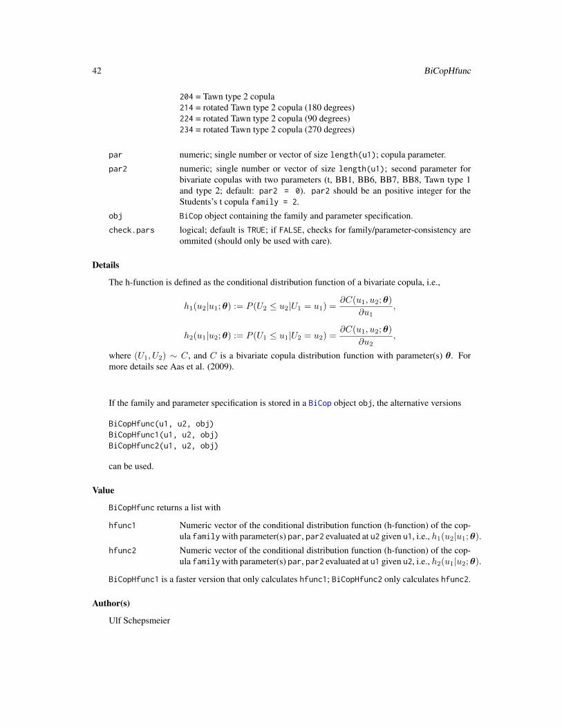
Details
The h-function is defined as the conditional distribution function of a bivariate copula, i.e.,
h1(u2|u1;θ) := P (U2 ≤ u2|U1 = u1) =∂C(u1, u2;θ)
∂u1,
h2(u1|u2;θ) := P (U1 ≤ u1|U2 = u2) =∂C(u1, u2;θ)
∂u2,
where (U1, U2) ∼ C, and C is a bivariate copula distribution function with parameter(s) θ. Formore details see Aas et al. (2009).
If the family and parameter specification is stored in a BiCop object obj, the alternative versions
BiCopHfunc(u1, u2, obj)BiCopHfunc1(u1, u2, obj)BiCopHfunc2(u1, u2, obj)
can be used.
Value
BiCopHfunc returns a list with
hfunc1 Numeric vector of the conditional distribution function (h-function) of the cop-ula family with parameter(s) par, par2 evaluated at u2 given u1, i.e., h1(u2|u1;θ).
hfunc2 Numeric vector of the conditional distribution function (h-function) of the cop-ula family with parameter(s) par, par2 evaluated at u1 given u2, i.e., h2(u1|u2;θ).
BiCopHfunc1 is a faster version that only calculates hfunc1; BiCopHfunc2 only calculates hfunc2.
Author(s)
Ulf Schepsmeier
BiCopHfuncDeriv 43
References
Aas, K., C. Czado, A. Frigessi, and H. Bakken (2009). Pair-copula constructions of multiple de-pendence. Insurance: Mathematics and Economics 44 (2), 182-198.
See Also
BiCopHinv, BiCopPDF, BiCopCDF, RVineLogLik, RVineSeqEst, BiCop
Examples
data(daxreturns)
# h-functions of the Gaussian copulacop <- BiCop(family = 1, par = 0.5)h <- BiCopHfunc(daxreturns[, 2], daxreturns[, 1], cop)
# or using the fast versionsh1 <- BiCopHfunc1(daxreturns[, 2], daxreturns[, 1], cop)h2 <- BiCopHfunc2(daxreturns[, 2], daxreturns[, 1], cop)all.equal(h$hfunc1, h1)all.equal(h$hfunc2, h2)
BiCopHfuncDeriv Derivatives of the h-Function of a Bivariate Copula
Description
This function evaluates the derivative of a given conditional parametric bivariate copula (h-function)with respect to its parameter(s) or one of its arguments.
Usage
BiCopHfuncDeriv(u1, u2, family, par, par2 = 0, deriv = "par", obj = NULL,check.pars = TRUE)
Arguments
u1, u2 numeric vectors of equal length with values in [0,1].
family integer; single number or vector of size length(u1); defines the bivariate cop-ula family: \cr 0 = independence copula1 = Gaussian copula2 = Student t copula (t-copula)3 = Clayton copula4 = Gumbel copula5 = Frank copula6 = Joe copula13 = rotated Clayton copula (180 degrees; “survival Clayton”)
44 BiCopHfuncDeriv
14 = rotated Gumbel copula (180 degrees; “survival Gumbel”)16 = rotated Joe copula (180 degrees; “survival Joe”)23 = rotated Clayton copula (90 degrees)24 = rotated Gumbel copula (90 degrees)26 = rotated Joe copula (90 degrees)33 = rotated Clayton copula (270 degrees)34 = rotated Gumbel copula (270 degrees)36 = rotated Joe copula (270 degrees)
par numeric; single number or vector of size length(u1); copula parameter.
par2 integer; single number or vector of size length(u1); second parameter for thet-Copula; default is par2 = 0, should be an positive integer for the Students’s tcopula family = 2.
deriv Derivative argument"par" = derivative with respect to the first parameter (default)"par2" = derivative with respect to the second parameter (only available for thet-copula)"u2" = derivative with respect to the second argument u2
obj BiCop object containing the family and parameter specification.
check.pars logical; default is TRUE; if FALSE, checks for family/parameter-consistency areommited (should only be used with care).
Details
If the family and parameter specification is stored in a BiCop object obj, the alternative version
BiCopHfuncDeriv(u1, u2, obj, deriv = "par")
can be used.
Value
A numeric vector of the conditional bivariate copula derivative
• of the copula family,
• with parameter(s) par, par2,
• with respect to deriv,
• evaluated at u1 and u2.
Author(s)
Ulf Schepsmeier
BiCopHfuncDeriv2 45
References
Schepsmeier, U. and J. Stoeber (2014). Derivatives and Fisher information of bivariate copulas.Statistical Papers, 55 (2), 525-542.http://link.springer.com/article/10.1007/s00362-013-0498-x.
See Also
RVineGrad, RVineHessian, BiCopDeriv2, BiCopDeriv2, BiCopHfuncDeriv, BiCop
Examples
## simulate from a bivariate Student-t copulaset.seed(123)cop <- BiCop(family = 2, par = -0.7, par2 = 4)simdata <- BiCopSim(100, cop)
## derivative of the conditional Student-t copula## with respect to the first parameteru1 <- simdata[,1]u2 <- simdata[,2]BiCopHfuncDeriv(u1, u2, cop, deriv = "par")
## estimate a Student-t copula for the simulated datacop <- BiCopEst(u1, u2, family = 2)## and evaluate the derivative of the conditional copula## w.r.t. the second argument u2BiCopHfuncDeriv(u1, u2, cop, deriv = "u2")
BiCopHfuncDeriv2 Second Derivatives of the h-Function of a Bivariate Copula
Description
This function evaluates the second derivative of a given conditional parametric bivariate copula(h-function) with respect to its parameter(s) and/or its arguments.
Usage
BiCopHfuncDeriv2(u1, u2, family, par, par2 = 0, deriv = "par", obj = NULL,check.pars = TRUE)
Arguments
u1, u2 numeric vectors of equal length with values in [0,1].
46 BiCopHfuncDeriv2
family integer; single number or vector of size length(u1); defines the bivariate cop-ula family:0 = independence copula1 = Gaussian copula2 = Student t copula (t-copula)3 = Clayton copula4 = Gumbel copula5 = Frank copula6 = Joe copula13 = rotated Clayton copula (180 degrees; “survival Clayton”)14 = rotated Gumbel copula (180 degrees; “survival Gumbel”)16 = rotated Joe copula (180 degrees; “survival Joe”)23 = rotated Clayton copula (90 degrees)24 = rotated Gumbel copula (90 degrees)26 = rotated Joe copula (90 degrees)33 = rotated Clayton copula (270 degrees)34 = rotated Gumbel copula (270 degrees)36 = rotated Joe copula (270 degrees)
par numeric; single number or vector of size length(u1); copula parameter.
par2 integer; single number or vector of size length(u1); second parameter for thet-Copula; default is par2 = 0, should be an positive integer for the Students’s tcopula family = 2.
deriv Derivative argument"par" = second derivative with respect to the first parameter (default)"par2" = second derivative with respect to the second parameter (only availablefor the t-copula)"u2" = second derivative with respect to the second argument u2"par1par2" = second derivative with respect to the first and second parameter(only available for the t-copula)"par1u2" = second derivative with respect to the first parameter and the secondargument"par2u2" = second derivative with respect to the second parameter and the sec-ond argument (only available for the t-copula)
obj BiCop object containing the family and parameter specification.
check.pars logical; default is TRUE; if FALSE, checks for family/parameter-consistency areommited (should only be used with care).
Details
If the family and parameter specification is stored in a BiCop object obj, the alternative version
BiCopHfuncDeriv2(u1, u2, obj, deriv = "par")
can be used.
BiCopHfuncDeriv2 47
Value
A numeric vector of the second-order conditional bivariate copula derivative
• of the copula family
• with parameter(s) par, par2
• with respect to deriv
• evaluated at u1 and u2.
Author(s)
Ulf Schepsmeier, Jakob Stoeber
References
Schepsmeier, U. and J. Stoeber (2014). Derivatives and Fisher information of bivariate copulas.Statistical Papers, 55 (2), 525-542.http://link.springer.com/article/10.1007/s00362-013-0498-x.
See Also
RVineGrad, RVineHessian, BiCopDeriv, BiCopDeriv2, BiCopHfuncDeriv, BiCop
Examples
## simulate from a bivariate Student-t copulaset.seed(123)cop <- BiCop(family = 2, par = -0.7, par2 = 4)simdata <- BiCopSim(100, cop)
## second derivative of the conditional bivariate t-copula## with respect to the first parameteru1 <- simdata[,1]u2 <- simdata[,2]BiCopHfuncDeriv2(u1, u2, cop, deriv = "par")
## estimate a Student-t copula for the simulated datacop <- BiCopEst(u1, u2, family = 2)## and evaluate the derivative of the conditional copula## w.r.t. the second argument u2BiCopHfuncDeriv2(u1, u2, cop, deriv = "u2")
48 BiCopHinv
BiCopHinv Inverse Conditional Distribution Function of a Bivariate Copula
Description
Evaluate the inverse conditional distribution function (inverse h-function) of a given parametricbivariate copula.
Usage
BiCopHinv(u1, u2, family, par, par2 = 0, obj = NULL, check.pars = TRUE)
BiCopHinv1(u1, u2, family, par, par2 = 0, obj = NULL, check.pars = TRUE)
BiCopHinv2(u1, u2, family, par, par2 = 0, obj = NULL, check.pars = TRUE)
Arguments
u1, u2 numeric vectors of equal length with values in [0,1].
family integer; single number or vector of size length(u1); defines the bivariate cop-ula family:0 = independence copula1 = Gaussian copula2 = Student t copula (t-copula)3 = Clayton copula4 = Gumbel copula5 = Frank copula6 = Joe copula7 = BB1 copula8 = BB6 copula9 = BB7 copula10 = BB8 copula13 = rotated Clayton copula (180 degrees; “survival Clayton”)14 = rotated Gumbel copula (180 degrees; “survival Gumbel”)16 = rotated Joe copula (180 degrees; “survival Joe”)17 = rotated BB1 copula (180 degrees; “survival BB1”)18 = rotated BB6 copula (180 degrees; “survival BB6”)19 = rotated BB7 copula (180 degrees; “survival BB7”)20 = rotated BB8 copula (180 degrees; “survival BB8”)23 = rotated Clayton copula (90 degrees)24 = rotated Gumbel copula (90 degrees)26 = rotated Joe copula (90 degrees)27 = rotated BB1 copula (90 degrees)28 = rotated BB6 copula (90 degrees)29 = rotated BB7 copula (90 degrees)30 = rotated BB8 copula (90 degrees)33 = rotated Clayton copula (270 degrees)
BiCopHinv 49
34 = rotated Gumbel copula (270 degrees)36 = rotated Joe copula (270 degrees)37 = rotated BB1 copula (270 degrees)38 = rotated BB6 copula (270 degrees)39 = rotated BB7 copula (270 degrees)40 = rotated BB8 copula (270 degrees)104 = Tawn type 1 copula114 = rotated Tawn type 1 copula (180 degrees)124 = rotated Tawn type 1 copula (90 degrees)134 = rotated Tawn type 1 copula (270 degrees)204 = Tawn type 2 copula214 = rotated Tawn type 2 copula (180 degrees)224 = rotated Tawn type 2 copula (90 degrees)234 = rotated Tawn type 2 copula (270 degrees)
par numeric; single number or vector of size length(u1); copula parameter.
par2 numeric; single number or vector of size length(u1); second parameter forbivariate copulas with two parameters (t, BB1, BB6, BB7, BB8, Tawn type 1and type 2; default: par2 = 0). par2 should be an positive integer for theStudents’s t copula family = 2.
obj BiCop object containing the family and parameter specification.
check.pars logical; default is TRUE; if FALSE, checks for family/parameter-consistency areommited (should only be used with care).
Details
The h-function is defined as the conditional distribution function of a bivariate copula, i.e.,
h1(u2|u1;θ) := P (U2 ≤ u2|U1 = u1) =∂C(u1, u2;θ)
∂u1,
h2(u1|u2;θ) := P (U1 ≤ u1|U2 = u2) =∂C(u1, u2;θ)
∂u2,
where (U1, U2) ∼ C, and C is a bivariate copula distribution function with parameter(s) θ. Formore details see Aas et al. (2009).
If the family and parameter specification is stored in a BiCop object obj, the alternative version
BiCopHinv(u1, u2, obj),BiCopHinv1(u1, u2, obj),BiCopHinv2(u1, u2, obj)
can be used.
50 BiCopHinv
Value
BiCopHinv returns a list with
hinv1 Numeric vector of the inverse conditional distribution function (inverse h-function)of the copula family with parameter(s) par, par2 evaluated at u2 given u1, i.e.,h−11 (u2|u1;θ).
hinv2 Numeric vector of the inverse conditional distribution function (inverse h-function)of the copula family with parameter(s) par, par2 evaluated at u1 given u2, i.e.,h−12 (u1|u2;θ).
BiCopHinv1 is a faster version that only calculates hinv1; BiCopHinv2 only calculates hinv2.
Author(s)
Ulf Schepsmeier, Thomas Nagler
References
Aas, K., C. Czado, A. Frigessi, and H. Bakken (2009). Pair-copula constructions of multiple de-pendence. Insurance: Mathematics and Economics 44 (2), 182-198.
See Also
BiCopHfunc, BiCopPDF, BiCopCDF, RVineLogLik, RVineSeqEst, BiCop
Examples
# inverse h-functions of the Gaussian copulacop <- BiCop(1, 0.5)hi <- BiCopHinv(0.1, 0.2, cop)
# or using the fast versionshi1 <- BiCopHinv1(0.1, 0.2, cop)hi2 <- BiCopHinv2(0.1, 0.2, cop)all.equal(hi$hinv1, hi1)all.equal(hi$hinv2, hi2)
# check if it is actually the inversecop <- BiCop(3, 3)all.equal(0.2, BiCopHfunc1(0.1, BiCopHinv1(0.1, 0.2, cop), cop))all.equal(0.1, BiCopHfunc2(BiCopHinv2(0.1, 0.2, cop), 0.2, cop))
BiCopIndTest 51
BiCopIndTest Independence Test for Bivariate Copula Data
Description
This function returns the p-value of a bivariate asymptotic independence test based on Kendall’s τ .
Usage
BiCopIndTest(u1, u2)
Arguments
u1, u2 Data vectors of equal length with values in [0,1].
Details
The test exploits the asymptotic normality of the test statistic
statistic := T =
√9N(N − 1)
2(2N + 5)× |τ |,
where N is the number of observations (length of u1) and τ the empirical Kendall’s tau of thedata vectors u1 and u2. The p-value of the null hypothesis of bivariate independence hence isasymptotically
p.value = 2× (1− Φ (T )) ,
where Φ is the standard normal distribution function.
Value
statistic Test statistic of the independence test.
p.value P-value of the independence test.
Author(s)
Jeffrey Dissmann
References
Genest, C. and A. C. Favre (2007). Everything you always wanted to know about copula modelingbut were afraid to ask. Journal of Hydrologic Engineering, 12 (4), 347-368.
See Also
BiCopGofTest, BiCopPar2Tau, BiCopTau2Par, BiCopSelect,RVineCopSelect, RVineStructureSelect
52 BiCopKDE
Examples
## Example 1: Gaussian copula with large dependence parametercop <- BiCop(1, 0.7)dat <- BiCopSim(500, cop)
# perform the asymptotic independence testBiCopIndTest(dat[, 1], dat[, 2])
## Example 2: Gaussian copula with small dependence parametercop <- BiCop(1, 0.01)dat <- BiCopSim(500, cop)
# perform the asymptotic independence testBiCopIndTest(dat[, 1], dat[, 2])
BiCopKDE Kernel estimate of a Bivariate Copula Density
Description
A kernel density estimate of the copula density is visualized. The function provides the same optionsas plot.BiCop. Further arguments can be passed to kdecop to modify the estimate.
Usage
BiCopKDE(u1, u2, type = "contour", margins, size, kde.pars = list(), ...)
Arguments
u1, u2 numeric vectors of equal length with values in [0,1].
type plot type; either "contour" or "surface" (partial matching is activated) for acontour or perspective/surface plot respectively.
margins only relevant for types "contour" and "surface"; options are: "unif" forthe original copula density, "norm" for the transformed density with standardnormal margins, "exp" with standard exponential margins, and "flexp" withflipped exponential margins. Default is "norm" for type = "contour", and"unif" for type = "surface". "norm" for the transformed density withstandard normal margins (partial matching is activated). Default is "norm" fortype = "contour", and "unif" for type = "surface".
size integer; the plot is based on values on a size x size grid; default is 100 fortype = "contour", and 25 for type = "surface".
kde.pars list of arguments passed to kdecop.
... optional arguments passed to contour or wireframe.
BiCopKPlot 53
Details
For further details on estimation see kdecop.
Author(s)
Thomas Nagler
Examples
# simulate data from Joe copulacop <- BiCop(3, tau = 0.3)u <- BiCopSim(1000, cop)contour(cop) # true contours
# kernel contours with standard normal marginsBiCopKDE(u[, 1], u[, 2])BiCopKDE(u[, 1], u[, 2], kde.pars = list(mult = 0.5)) # undersmoothBiCopKDE(u[, 1], u[, 2], kde.pars = list(mult = 2)) # oversmooth
# kernel density with uniform marginsBiCopKDE(u[, 1], u[, 2], type = "surface", zlim = c(0, 4))plot(cop, zlim = c(0, 4)) # true density
# kernel contours are also used in pairs.copuladatadata(daxreturns)data <- as.copuladata(daxreturns)pairs(data[c(4, 5, 14, 15)])
BiCopKPlot Kendall’s Plot for Bivariate Copula Data
Description
This function creates a Kendall’s plot (K-plot) of given bivariate copula data.
Usage
BiCopKPlot(u1, u2, PLOT = TRUE, ...)
Arguments
u1, u2 Data vectors of equal length with values in [0,1].
PLOT Logical; whether the results are plotted. If PLOT = FALSE, the values W.in andHi.sort are returned (see below; default: PLOT = TRUE).
... Additional plot arguments.
54 BiCopKPlot
Details
For observations ui,j , i = 1, ..., N, j = 1, 2, the K-plot considers two quantities: First, the orderedvalues of the empirical bivariate distribution function Hi := FU1U2
(ui,1, ui,2) and, second, Wi:N ,which are the expected values of the order statistics from a random sample of size N of the randomvariable W = C(U1, U2) under the null hypothesis of independence between U1 and U2. Wi:N canbe calculated as follows
Wi:n = N
(N − 1
i− 1
) 1∫0
ωk0(ω)(K0(ω))i−1(1−K0(ω))N−idω,
whereK0(ω) = ω − ω log(ω),
and k0(·) is the corresponding density.
K-plots can be seen as the bivariate copula equivalent to QQ-plots. If the points of a K-plot lie ap-proximately on the diagonal y = x, then U1 and U2 are approximately independent. Any deviationfrom the diagonal line points towards dependence. In case of positive dependence, the points ofthe K-plot should be located above the diagonal line, and vice versa for negative dependence. Thelarger the deviation from the diagonal, the stronger is the degree of dependency. There is a perfectpositive dependence if points (Wi:N , Hi) lie on the curve K0(ω) located above the main diagonal.If points (Wi:N , Hi) however lie on the x-axis, this indicates a perfect negative dependence betweenU1 and U2.
Value
W.in W-statistics (x-axis).
Hi.sort H-statistics (y-axis).
Author(s)
Natalia Belgorodski, Ulf Schepsmeier
References
Genest, C. and A. C. Favre (2007). Everything you always wanted to know about copula modelingbut were afraid to ask. Journal of Hydrologic Engineering, 12 (4), 347-368.
See Also
BiCopMetaContour, BiCopChiPlot, BiCopLambda, BiCopGofTest
Examples
## Gaussian and Clayton copulasn <- 500tau <- 0.5
# simulate from Gaussian copula
BiCopLambda 55
fam <- 1par <- BiCopTau2Par(fam, tau)cop1 <- BiCop(fam, par)set.seed(123)dat1 <- BiCopSim(n, cop1)
# simulate from Clayton copulafam <- 3par <- BiCopTau2Par(fam, tau)cop2 <- BiCop(fam, par)set.seed(123)dat2 <- BiCopSim(n, cop2)
# create K-plotsop <- par(mfrow = c(1, 2))BiCopKPlot(dat1[,1], dat1[,2], main = "Gaussian copula")BiCopKPlot(dat2[,1], dat2[,2], main = "Clayton copula")par(op)
BiCopLambda Lambda-Function (Plot) for Bivariate Copula Data
Description
This function plots/returns the lambda-function of given bivariate copula data.
Usage
BiCopLambda(u1 = NULL, u2 = NULL, family = "emp", par = 0, par2 = 0,PLOT = TRUE, obj = NULL, ...)
Arguments
u1, u2 Data vectors of equal length with values in [0,1] (default: u1 and u2 = NULL).
family An integer defining the bivariate copula family or indicating the empirical lambda-function:"emp" = empirical lambda-function (default)1 = Gaussian copula; the theoretical lambda-function is simulated (no closedformula available)2 = Student-t copula; the theoretical lambda-function is simulated (no closedformula available)3 = Clayton copula4 = Gumbel copula5 = Frank copula6 = Joe copula7 = BB1 copula8 = BB6 copula
56 BiCopLambda
9 = BB7 copula10 = BB8 copula
par Copula parameter; if the empirical lambda-function is chosen, par = NULL or 0(default).
par2 Second copula parameter for t-, BB1, BB6, BB7 and BB8 copulas (default:par2 = 0).
PLOT Logical; whether the results are plotted. If PLOT = FALSE, the valuesempLambda and/or theoLambda are returned (see below; default: PLOT = TRUE).
obj BiCop object containing the family and parameter specification.
... Additional plot arguments.
Details
If the family and parameter specification is stored in a BiCop object obj, the alternative versions
BiCopLambda(obj, PLOT = TRUE, ...)
and
BiCopLambda((u1, u2, obj, PLOT = TRUE, ...)
can be used.
Value
empLambda If the empirical lambda-function is chosen and PLOT = FALSE, a vector of theempirical lambda’s is returned.
theoLambda If the theoretical lambda-function is chosen and PLOT = FALSE, a vector of thetheoretical lambda’s is returned.
Note
The λ-function is characteristic for each bivariate copula family and defined by Kendall’s distribu-tion function K:
λ(v, θ) := v −K(v, θ)
withK(v, θ) := P (Cθ(U1, U2) ≤ v), v ∈ [0, 1].
For Archimedean copulas one has the following closed form expression in terms of the generatorfunction ϕ of the copula Cθ:
λ(v, θ) =ϕ(v)
ϕ′(v),
where ϕ′ is the derivative of ϕ. For more details see Genest and Rivest (1993) or Schepsmeier(2010).
For the bivariate Gaussian and Student-t copula no closed form expression for the theoretical λ-function exists. Therefore it is simulated based on samples of size 1000. For all other implementedcopula families there are closed form expressions available.
BiCopMetaContour 57
The plot of the theoretical λ-function also shows the limits of the λ-function corresponding toKendall’s tau = 0 and Kendall’s tau = 1 (λ = 0).
For rotated bivariate copulas one has to transform the input arguments u1 and/or u2. In particular,for copulas rotated by 90 degrees u1 has to be set to 1-u1, for 270 degrees u2 to 1-u2 and forsurvival copulas u1 and u2 to 1-u1 and 1-u2, respectively. Then λ-functions for the correspondingnon-rotated copula families can be considered.
Author(s)
Ulf Schepsmeier
References
Genest, C. and L.-P. Rivest (1993). Statistical inference procedures for bivariate Archimedeancopulas. Journal of the American Statistical Association, 88 (423), 1034-1043.
Schepsmeier, U. (2010). Maximum likelihood estimation of C-vine pair-copula constructions basedon bivariate copulas from different families. Diploma thesis, Technische Universitaet Muenchen.http://mediatum.ub.tum.de/?id=1079296.
See Also
BiCopMetaContour, BiCopKPlot, BiCopChiPlot, BiCop
Examples
# simulate from Clayton copulacop <- BiCop(3, tau = 0.5)dat <- BiCopSim(1000, cop)
# create lambda-function plotsop <- par(mfrow = c(1, 3))BiCopLambda(dat[, 1], dat[, 2]) # empirical lambda-functionBiCopLambda(cop) # theoretical lambda-functionBiCopLambda(dat[, 1], dat[, 2], cop) # bothpar(op)
BiCopMetaContour Contour Plot of Bivariate Meta Distribution
Description
Note: This function is deprecated and only available for backwards compatibility. See contour.BiCopfor contour plots of parametric copulas, and BiCopKDE for kernel estimates.
58 BiCopMetaContour
Usage
BiCopMetaContour(u1 = NULL, u2 = NULL, bw = 1, size = 100,levels = c(0.01, 0.05, 0.1, 0.15, 0.2), family = "emp", par = 0,par2 = 0, PLOT = TRUE, margins = "norm", margins.par = 0,xylim = NA, obj = NULL, ...)
Arguments
u1, u2 Data vectors of equal length with values in [0,1] (default: u1 and u2 = NULL).
bw Bandwidth (smoothing factor; default: bw = 1).
size Number of grid points; default: size = 100.
levels Vector of contour levels. For Gaussian, Student-t or exponential margins thedefault value (levels = c(0.01, 0.05, 0.1,0.15, 0.2)) typically is a goodchoice. For uniform margins we recommendlevels = c(0.1, 0.3, 0.5, 0.7, 0.9, 1.1, 1.3, 1.5)and for Gamma marginslevels = c(0.005, 0.01, 0.03, 0.05, 0.07,0.09).
family An integer defining the bivariate copula family or indicating an empirical con-tour plot:"emp" = empirical contour plot (default; margins can be specified by margins)0 = independence copula1 = Gaussian copula2 = Student t copula (t-copula)3 = Clayton copula4 = Gumbel copula5 = Frank copula6 = Joe copula7 = BB1 copula8 = BB6 copula9 = BB7 copula10 = BB8 copula13 = rotated Clayton copula (180 degrees; “survival Clayton”)14 = rotated Gumbel copula (180 degrees; “survival Gumbel”)16 = rotated Joe copula (180 degrees; “survival Joe”)17 = rotated BB1 copula (180 degrees; “survival BB1”)18 = rotated BB6 copula (180 degrees; “survival BB6”)19 = rotated BB7 copula (180 degrees; “survival BB7”)20 = rotated BB8 copula (180 degrees; “survival BB8”)23 = rotated Clayton copula (90 degrees)24 = rotated Gumbel copula (90 degrees)26 = rotated Joe copula (90 degrees)27 = rotated BB1 copula (90 degrees)28 = rotated BB6 copula (90 degrees)29 = rotated BB7 copula (90 degrees)30 = rotated BB8 copula (90 degrees)33 = rotated Clayton copula (270 degrees)34 = rotated Gumbel copula (270 degrees)
BiCopMetaContour 59
36 = rotated Joe copula (270 degrees)37 = rotated BB1 copula (270 degrees)38 = rotated BB6 copula (270 degrees)39 = rotated BB7 copula (270 degrees)40 = rotated BB8 copula (270 degrees)104 = Tawn type 1 copula114 = rotated Tawn type 1 copula (180 degrees)124 = rotated Tawn type 1 copula (90 degrees)134 = rotated Tawn type 1 copula (270 degrees)204 = Tawn type 2 copula214 = rotated Tawn type 2 copula (180 degrees)224 = rotated Tawn type 2 copula (90 degrees)234 = rotated Tawn type 2 copula (270 degrees)
par Copula parameter; if empirical contour plot, par = NULL or 0 (default).
par2 Second copula parameter for t-, BB1, BB6, BB7, BB8, Tawn type 1 and type 2copulas (default: par2 = 0).
PLOT Logical; whether the results are plotted. If PLOT = FALSE, the values x, y and zare returned (see below; default: PLOT = TRUE).
margins Character; margins for the bivariate copula contour plot. Possible margins are:"norm" = standard normal margins (default)"t" = Student t margins with degrees of freedom as specified by margins.par"gamma" = Gamma margins with shape and scale as specified by margins.par"exp" = Exponential margins with rate as specified by margins.par"unif" = uniform margins
margins.par Parameter(s) of the distribution of the margins if necessary (default: margins.par = 0),i.e.,
• a positive real number for the degrees of freedom of Student t margins (seedt),
• a 2-dimensional vector of positive real numbers for the shape and scaleparameters of Gamma margins (see dgamma),
• a positive real number for the rate parameter of exponential margins (seedexp).
xylim A 2-dimensional vector of the x- and y-limits. By default (xylim = NA) standardlimits for the selected margins are used.
obj BiCop object containing the family and parameter specification.
... Additional plot arguments.
Value
x A vector of length size with the x-values of the kernel density estimator withGaussian kernel if the empirical contour plot is chosen and a sequence of valuesin xylim if the theoretical contour plot is chosen.
y A vector of length size with the y-values of the kernel density estimator withGaussian kernel if the empirical contour plot is chosen and a sequence of valuesin xylim if the theoretical contour plot is chosen.
60 BiCopName
z A matrix of dimension size with the values of the density of the meta distribu-tion with chosen margins (see margins and margins.par) evaluated at the gridpoints given by x and y.
Note
The combination family = 0 (independence copula) and margins = "unif" (uniform margins)is not possible because all z-values are equal.
Author(s)
Ulf Schepsmeier, Alexander Bauer
See Also
BiCopChiPlot, BiCopKPlot, BiCopLambda
Examples
## meta Clayton distribution with Gaussian marginscop <- BiCop(family = 1, tau = 0.5)BiCopMetaContour(obj = cop, main = "Clayton - normal margins")# better:contour(cop, main = "Clayton - normal margins")
## empirical contour plot with standard normal marginsdat <- BiCopSim(1000, cop)BiCopMetaContour(dat[, 1], dat[, 2], bw = 2, family = "emp",
main = "empirical - normal margins")# better:BiCopKDE(dat[, 1], dat[, 2],
main = "empirical - normal margins")
## empirical contour plot with exponential marginsBiCopMetaContour(dat[, 1], dat[, 2], bw = 2,
main = "empirical - exponential margins",margins = "exp", margins.par = 1)
# better:BiCopKDE(dat[, 1], dat[, 2],
main = "empirical - exponential margins",margins = "exp")
BiCopName Bivariate Copula Family Names
Description
This function transforms the bivariate copula family number into its character expression and viceversa.
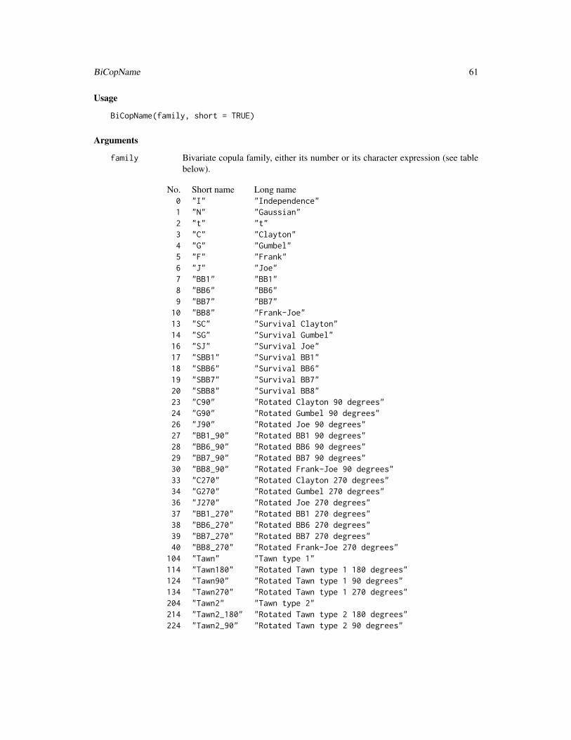
BiCopName 61
Usage
BiCopName(family, short = TRUE)
Arguments
family Bivariate copula family, either its number or its character expression (see tablebelow).
No. Short name Long name0 "I" "Independence"1 "N" "Gaussian"2 "t" "t"3 "C" "Clayton"4 "G" "Gumbel"5 "F" "Frank"6 "J" "Joe"7 "BB1" "BB1"8 "BB6" "BB6"9 "BB7" "BB7"10 "BB8" "Frank-Joe"13 "SC" "Survival Clayton"14 "SG" "Survival Gumbel"16 "SJ" "Survival Joe"17 "SBB1" "Survival BB1"18 "SBB6" "Survival BB6"19 "SBB7" "Survival BB7"20 "SBB8" "Survival BB8"23 "C90" "Rotated Clayton 90 degrees"24 "G90" "Rotated Gumbel 90 degrees"26 "J90" "Rotated Joe 90 degrees"27 "BB1_90" "Rotated BB1 90 degrees"28 "BB6_90" "Rotated BB6 90 degrees"29 "BB7_90" "Rotated BB7 90 degrees"30 "BB8_90" "Rotated Frank-Joe 90 degrees"33 "C270" "Rotated Clayton 270 degrees"34 "G270" "Rotated Gumbel 270 degrees"36 "J270" "Rotated Joe 270 degrees"37 "BB1_270" "Rotated BB1 270 degrees"38 "BB6_270" "Rotated BB6 270 degrees"39 "BB7_270" "Rotated BB7 270 degrees"40 "BB8_270" "Rotated Frank-Joe 270 degrees"104 "Tawn" "Tawn type 1"114 "Tawn180" "Rotated Tawn type 1 180 degrees"124 "Tawn90" "Rotated Tawn type 1 90 degrees"134 "Tawn270" "Rotated Tawn type 1 270 degrees"204 "Tawn2" "Tawn type 2"214 "Tawn2_180" "Rotated Tawn type 2 180 degrees"224 "Tawn2_90" "Rotated Tawn type 2 90 degrees"
62 BiCopPar2Beta
234 "Tawn2_270" "Rotated Tawn type 2 270 degrees"
short Logical; if the number of a bivariate copula family is used and short = TRUE(default), a short version of the corresponding character expression is returned,otherwise the long version.
Value
The transformed bivariate copula family (see table above).
Author(s)
Ulf Schepsmeier
See Also
RVineTreePlot
Examples
## family number to character expressionfamily <- 1BiCopName(family, short = TRUE) # short versionBiCopName(family, short = FALSE) # long version
## family character expression (short version) to numberfamily <- "C"BiCopName(family) # as number
## family character expression (long version) to numberfamily <- "Clayton"BiCopName(family) # as number
## vectors of familiesBiCopName(1:10) # as character expressionBiCopName(c("Clayton","t","J")) # as number
BiCopPar2Beta Blomqvist’s Beta Value of a Bivariate Copula
Description
This function computes the theoretical Blomqvist’s beta value of a bivariate copula for given pa-rameter values.
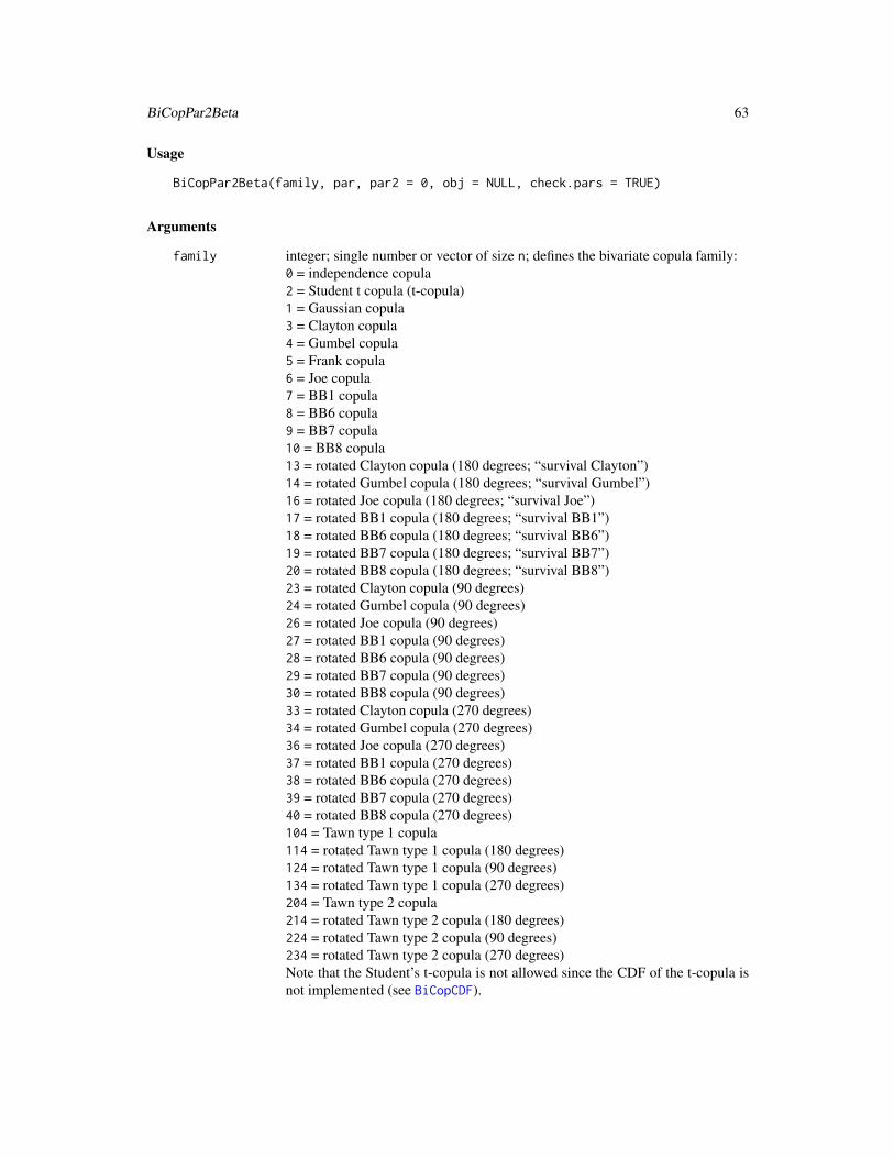
BiCopPar2Beta 63
Usage
BiCopPar2Beta(family, par, par2 = 0, obj = NULL, check.pars = TRUE)
Arguments
family integer; single number or vector of size n; defines the bivariate copula family:0 = independence copula2 = Student t copula (t-copula)1 = Gaussian copula3 = Clayton copula4 = Gumbel copula5 = Frank copula6 = Joe copula7 = BB1 copula8 = BB6 copula9 = BB7 copula10 = BB8 copula13 = rotated Clayton copula (180 degrees; “survival Clayton”)14 = rotated Gumbel copula (180 degrees; “survival Gumbel”)16 = rotated Joe copula (180 degrees; “survival Joe”)17 = rotated BB1 copula (180 degrees; “survival BB1”)18 = rotated BB6 copula (180 degrees; “survival BB6”)19 = rotated BB7 copula (180 degrees; “survival BB7”)20 = rotated BB8 copula (180 degrees; “survival BB8”)23 = rotated Clayton copula (90 degrees)24 = rotated Gumbel copula (90 degrees)26 = rotated Joe copula (90 degrees)27 = rotated BB1 copula (90 degrees)28 = rotated BB6 copula (90 degrees)29 = rotated BB7 copula (90 degrees)30 = rotated BB8 copula (90 degrees)33 = rotated Clayton copula (270 degrees)34 = rotated Gumbel copula (270 degrees)36 = rotated Joe copula (270 degrees)37 = rotated BB1 copula (270 degrees)38 = rotated BB6 copula (270 degrees)39 = rotated BB7 copula (270 degrees)40 = rotated BB8 copula (270 degrees)104 = Tawn type 1 copula114 = rotated Tawn type 1 copula (180 degrees)124 = rotated Tawn type 1 copula (90 degrees)134 = rotated Tawn type 1 copula (270 degrees)204 = Tawn type 2 copula214 = rotated Tawn type 2 copula (180 degrees)224 = rotated Tawn type 2 copula (90 degrees)234 = rotated Tawn type 2 copula (270 degrees)Note that the Student’s t-copula is not allowed since the CDF of the t-copula isnot implemented (see BiCopCDF).
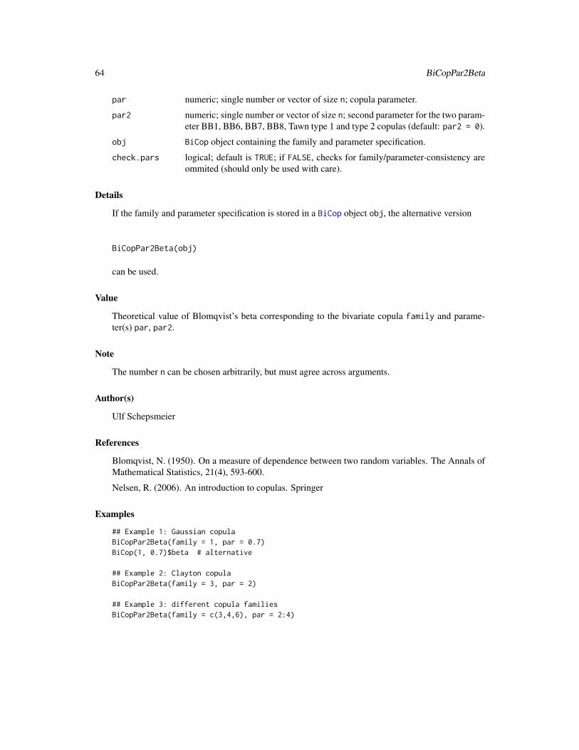
64 BiCopPar2Beta
par numeric; single number or vector of size n; copula parameter.
par2 numeric; single number or vector of size n; second parameter for the two param-eter BB1, BB6, BB7, BB8, Tawn type 1 and type 2 copulas (default: par2 = 0).
obj BiCop object containing the family and parameter specification.
check.pars logical; default is TRUE; if FALSE, checks for family/parameter-consistency areommited (should only be used with care).
Details
If the family and parameter specification is stored in a BiCop object obj, the alternative version
BiCopPar2Beta(obj)
can be used.
Value
Theoretical value of Blomqvist’s beta corresponding to the bivariate copula family and parame-ter(s) par, par2.
Note
The number n can be chosen arbitrarily, but must agree across arguments.
Author(s)
Ulf Schepsmeier
References
Blomqvist, N. (1950). On a measure of dependence between two random variables. The Annals ofMathematical Statistics, 21(4), 593-600.
Nelsen, R. (2006). An introduction to copulas. Springer
Examples
## Example 1: Gaussian copulaBiCopPar2Beta(family = 1, par = 0.7)BiCop(1, 0.7)$beta # alternative
## Example 2: Clayton copulaBiCopPar2Beta(family = 3, par = 2)
## Example 3: different copula familiesBiCopPar2Beta(family = c(3,4,6), par = 2:4)
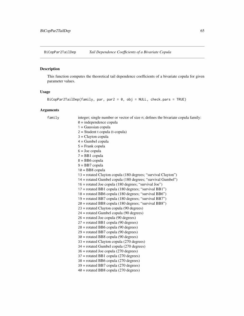
BiCopPar2TailDep 65
BiCopPar2TailDep Tail Dependence Coefficients of a Bivariate Copula
Description
This function computes the theoretical tail dependence coefficients of a bivariate copula for givenparameter values.
Usage
BiCopPar2TailDep(family, par, par2 = 0, obj = NULL, check.pars = TRUE)
Arguments
family integer; single number or vector of size n; defines the bivariate copula family:0 = independence copula1 = Gaussian copula2 = Student t copula (t-copula)3 = Clayton copula4 = Gumbel copula5 = Frank copula6 = Joe copula7 = BB1 copula8 = BB6 copula9 = BB7 copula10 = BB8 copula13 = rotated Clayton copula (180 degrees; “survival Clayton”)14 = rotated Gumbel copula (180 degrees; “survival Gumbel”)16 = rotated Joe copula (180 degrees; “survival Joe”)17 = rotated BB1 copula (180 degrees; “survival BB1”)18 = rotated BB6 copula (180 degrees; “survival BB6”)19 = rotated BB7 copula (180 degrees; “survival BB7”)20 = rotated BB8 copula (180 degrees; “survival BB8”)23 = rotated Clayton copula (90 degrees)24 = rotated Gumbel copula (90 degrees)26 = rotated Joe copula (90 degrees)27 = rotated BB1 copula (90 degrees)28 = rotated BB6 copula (90 degrees)29 = rotated BB7 copula (90 degrees)30 = rotated BB8 copula (90 degrees)33 = rotated Clayton copula (270 degrees)34 = rotated Gumbel copula (270 degrees)36 = rotated Joe copula (270 degrees)37 = rotated BB1 copula (270 degrees)38 = rotated BB6 copula (270 degrees)39 = rotated BB7 copula (270 degrees)40 = rotated BB8 copula (270 degrees)
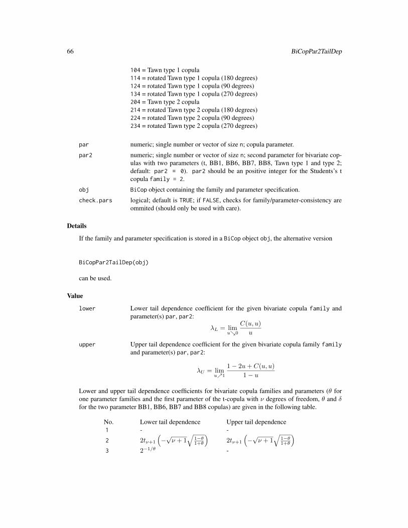
66 BiCopPar2TailDep
104 = Tawn type 1 copula114 = rotated Tawn type 1 copula (180 degrees)124 = rotated Tawn type 1 copula (90 degrees)134 = rotated Tawn type 1 copula (270 degrees)204 = Tawn type 2 copula214 = rotated Tawn type 2 copula (180 degrees)224 = rotated Tawn type 2 copula (90 degrees)234 = rotated Tawn type 2 copula (270 degrees)
par numeric; single number or vector of size n; copula parameter.
par2 numeric; single number or vector of size n; second parameter for bivariate cop-ulas with two parameters (t, BB1, BB6, BB7, BB8, Tawn type 1 and type 2;default: par2 = 0). par2 should be an positive integer for the Students’s tcopula family = 2.
obj BiCop object containing the family and parameter specification.
check.pars logical; default is TRUE; if FALSE, checks for family/parameter-consistency areommited (should only be used with care).
Details
If the family and parameter specification is stored in a BiCop object obj, the alternative version
BiCopPar2TailDep(obj)
can be used.
Value
lower Lower tail dependence coefficient for the given bivariate copula family andparameter(s) par, par2:
λL = limu↘0
C(u, u)
u
upper Upper tail dependence coefficient for the given bivariate copula family familyand parameter(s) par, par2:
λU = limu↗1
1− 2u+ C(u, u)
1− u
Lower and upper tail dependence coefficients for bivariate copula families and parameters (θ forone parameter families and the first parameter of the t-copula with ν degrees of freedom, θ and δfor the two parameter BB1, BB6, BB7 and BB8 copulas) are given in the following table.
No. Lower tail dependence Upper tail dependence1 - -
2 2tν+1
(−√ν + 1
√1−θ1+θ
)2tν+1
(−√ν + 1
√1−θ1+θ
)3 2−1/θ -
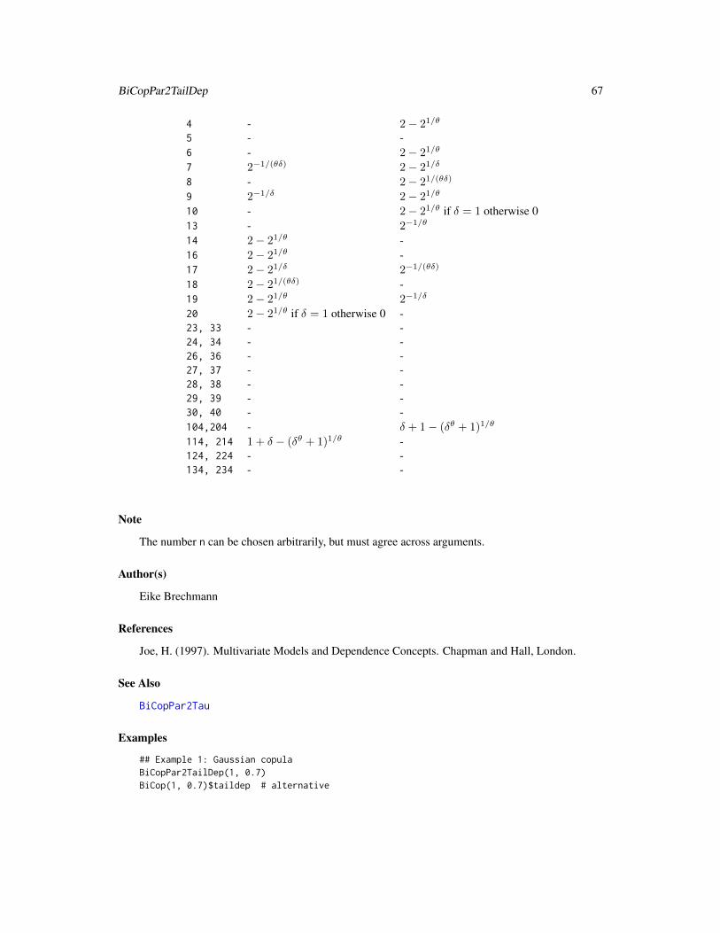
BiCopPar2TailDep 67
4 - 2− 21/θ
5 - -6 - 2− 21/θ
7 2−1/(θδ) 2− 21/δ
8 - 2− 21/(θδ)
9 2−1/δ 2− 21/θ
10 - 2− 21/θ if δ = 1 otherwise 013 - 2−1/θ
14 2− 21/θ -16 2− 21/θ -17 2− 21/δ 2−1/(θδ)
18 2− 21/(θδ) -19 2− 21/θ 2−1/δ
20 2− 21/θ if δ = 1 otherwise 0 -23, 33 - -24, 34 - -26, 36 - -27, 37 - -28, 38 - -29, 39 - -30, 40 - -104,204 - δ + 1− (δθ + 1)1/θ
114, 214 1 + δ − (δθ + 1)1/θ -124, 224 - -134, 234 - -
Note
The number n can be chosen arbitrarily, but must agree across arguments.
Author(s)
Eike Brechmann
References
Joe, H. (1997). Multivariate Models and Dependence Concepts. Chapman and Hall, London.
See Also
BiCopPar2Tau
Examples
## Example 1: Gaussian copulaBiCopPar2TailDep(1, 0.7)BiCop(1, 0.7)$taildep # alternative
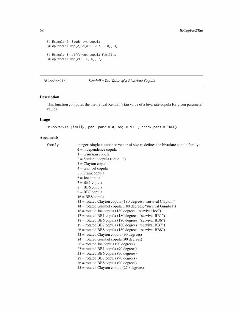
68 BiCopPar2Tau
## Example 2: Student-t copulaBiCopPar2TailDep(2, c(0.6, 0.7, 0.8), 4)
## Example 3: different copula familiesBiCopPar2TailDep(c(3, 4, 6), 2)
BiCopPar2Tau Kendall’s Tau Value of a Bivariate Copula
Description
This function computes the theoretical Kendall’s tau value of a bivariate copula for given parametervalues.
Usage
BiCopPar2Tau(family, par, par2 = 0, obj = NULL, check.pars = TRUE)
Arguments
family integer; single number or vector of size m; defines the bivariate copula family:0 = independence copula1 = Gaussian copula2 = Student t copula (t-copula)3 = Clayton copula4 = Gumbel copula5 = Frank copula6 = Joe copula7 = BB1 copula8 = BB6 copula9 = BB7 copula10 = BB8 copula13 = rotated Clayton copula (180 degrees; “survival Clayton”)14 = rotated Gumbel copula (180 degrees; “survival Gumbel”)16 = rotated Joe copula (180 degrees; “survival Joe”)17 = rotated BB1 copula (180 degrees; “survival BB1”)18 = rotated BB6 copula (180 degrees; “survival BB6”)19 = rotated BB7 copula (180 degrees; “survival BB7”)20 = rotated BB8 copula (180 degrees; “survival BB8”)23 = rotated Clayton copula (90 degrees)24 = rotated Gumbel copula (90 degrees)26 = rotated Joe copula (90 degrees)27 = rotated BB1 copula (90 degrees)28 = rotated BB6 copula (90 degrees)29 = rotated BB7 copula (90 degrees)30 = rotated BB8 copula (90 degrees)33 = rotated Clayton copula (270 degrees)
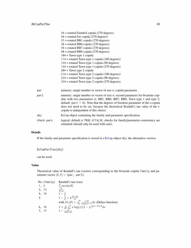
BiCopPar2Tau 69
34 = rotated Gumbel copula (270 degrees)36 = rotated Joe copula (270 degrees)37 = rotated BB1 copula (270 degrees)38 = rotated BB6 copula (270 degrees)39 = rotated BB7 copula (270 degrees)40 = rotated BB8 copula (270 degrees)104 = Tawn type 1 copula114 = rotated Tawn type 1 copula (180 degrees)124 = rotated Tawn type 1 copula (90 degrees)134 = rotated Tawn type 1 copula (270 degrees)204 = Tawn type 2 copula214 = rotated Tawn type 2 copula (180 degrees)224 = rotated Tawn type 2 copula (90 degrees)234 = rotated Tawn type 2 copula (270 degrees)
par numeric; single number or vector of size n; copula parameter.
par2 numeric; single number or vector of size n; second parameter for bivariate cop-ulas with two parameters (t, BB1, BB6, BB7, BB8, Tawn type 1 and type 2;default: par2 = 0). Note that the degrees of freedom parameter of the t-copuladoes not need to be set, because the theoretical Kendall’s tau value of the t-copula is independent of this choice.
obj BiCop object containing the family and parameter specification.
check.pars logical; default is TRUE; if FALSE, checks for family/parameter-consistency areommited (should only be used with care).
Details
If the family and parameter specification is stored in a BiCop object obj, the alternative version
BiCopPar2Tau(obj)
can be used.
Value
Theoretical value of Kendall’s tau (vector) corresponding to the bivariate copula family and pa-rameter vector (θ, δ) = (par, par2).
No. (family) Kendall’s tau (tau)1, 2 2
π arcsin(θ)3, 13 θ
θ+2
4, 14 1− 1θ
5 1− 4θ + 4D1(θ)
θ
with D1(θ) =∫ θ0
x/θexp(x)−1dx (Debye function)
6, 16 1 + 4θ2
∫ 1
0x log(x)(1− x)2(1−θ)/θdx
7, 17 1− 2δ(θ+2)
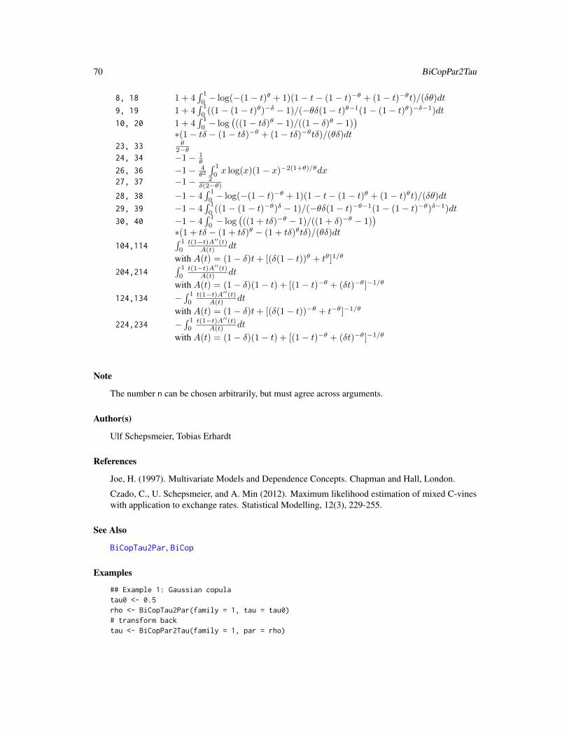
70 BiCopPar2Tau
8, 18 1 + 4∫ 1
0− log(−(1− t)θ + 1)(1− t− (1− t)−θ + (1− t)−θt)/(δθ)dt
9, 19 1 + 4∫ 1
0((1− (1− t)θ)−δ − 1)/(−θδ(1− t)θ−1(1− (1− t)θ)−δ−1)dt
10, 20 1 + 4∫ 1
0− log
(((1− tδ)θ − 1)/((1− δ)θ − 1)
)∗(1− tδ − (1− tδ)−θ + (1− tδ)−θtδ)/(θδ)dt
23, 33 θ2−θ
24, 34 −1− 1θ
26, 36 −1− 4θ2
∫ 1
0x log(x)(1− x)−2(1+θ)/θdx
27, 37 −1− 2δ(2−θ)
28, 38 −1− 4∫ 1
0− log(−(1− t)−θ + 1)(1− t− (1− t)θ + (1− t)θt)/(δθ)dt
29, 39 −1− 4∫ 1
0((1− (1− t)−θ)δ − 1)/(−θδ(1− t)−θ−1(1− (1− t)−θ)δ−1)dt
30, 40 −1− 4∫ 1
0− log
(((1 + tδ)−θ − 1)/((1 + δ)−θ − 1)
)∗(1 + tδ − (1 + tδ)θ − (1 + tδ)θtδ)/(θδ)dt
104,114∫ 1
0t(1−t)A′′(t)
A(t) dt
with A(t) = (1− δ)t+ [(δ(1− t))θ + tθ]1/θ
204,214∫ 1
0t(1−t)A′′(t)
A(t) dt
with A(t) = (1− δ)(1− t) + [(1− t)−θ + (δt)−θ]−1/θ
124,134 −∫ 1
0t(1−t)A′′(t)
A(t) dt
with A(t) = (1− δ)t+ [(δ(1− t))−θ + t−θ]−1/θ
224,234 −∫ 1
0t(1−t)A′′(t)
A(t) dt
with A(t) = (1− δ)(1− t) + [(1− t)−θ + (δt)−θ]−1/θ
Note
The number n can be chosen arbitrarily, but must agree across arguments.
Author(s)
Ulf Schepsmeier, Tobias Erhardt
References
Joe, H. (1997). Multivariate Models and Dependence Concepts. Chapman and Hall, London.
Czado, C., U. Schepsmeier, and A. Min (2012). Maximum likelihood estimation of mixed C-vineswith application to exchange rates. Statistical Modelling, 12(3), 229-255.
See Also
BiCopTau2Par, BiCop
Examples
## Example 1: Gaussian copulatau0 <- 0.5rho <- BiCopTau2Par(family = 1, tau = tau0)# transform backtau <- BiCopPar2Tau(family = 1, par = rho)
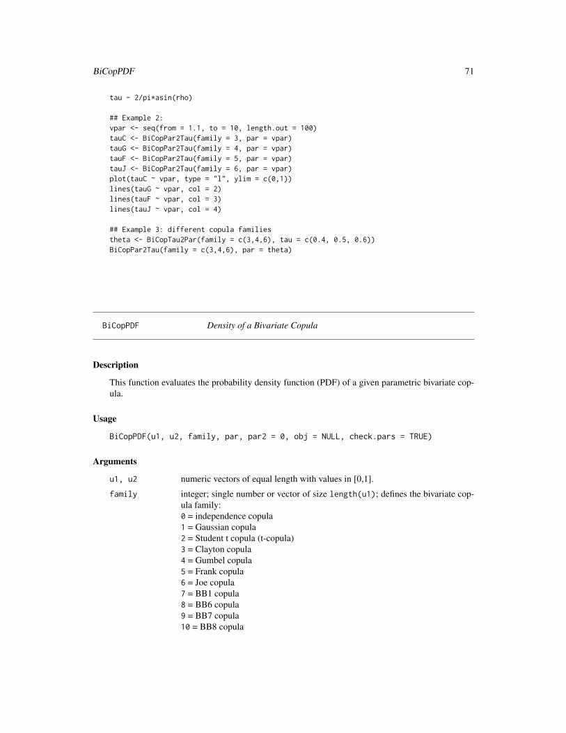
BiCopPDF 71
tau - 2/pi*asin(rho)
## Example 2:vpar <- seq(from = 1.1, to = 10, length.out = 100)tauC <- BiCopPar2Tau(family = 3, par = vpar)tauG <- BiCopPar2Tau(family = 4, par = vpar)tauF <- BiCopPar2Tau(family = 5, par = vpar)tauJ <- BiCopPar2Tau(family = 6, par = vpar)plot(tauC ~ vpar, type = "l", ylim = c(0,1))lines(tauG ~ vpar, col = 2)lines(tauF ~ vpar, col = 3)lines(tauJ ~ vpar, col = 4)
## Example 3: different copula familiestheta <- BiCopTau2Par(family = c(3,4,6), tau = c(0.4, 0.5, 0.6))BiCopPar2Tau(family = c(3,4,6), par = theta)
BiCopPDF Density of a Bivariate Copula
Description
This function evaluates the probability density function (PDF) of a given parametric bivariate cop-ula.
Usage
BiCopPDF(u1, u2, family, par, par2 = 0, obj = NULL, check.pars = TRUE)
Arguments
u1, u2 numeric vectors of equal length with values in [0,1].
family integer; single number or vector of size length(u1); defines the bivariate cop-ula family:0 = independence copula1 = Gaussian copula2 = Student t copula (t-copula)3 = Clayton copula4 = Gumbel copula5 = Frank copula6 = Joe copula7 = BB1 copula8 = BB6 copula9 = BB7 copula10 = BB8 copula
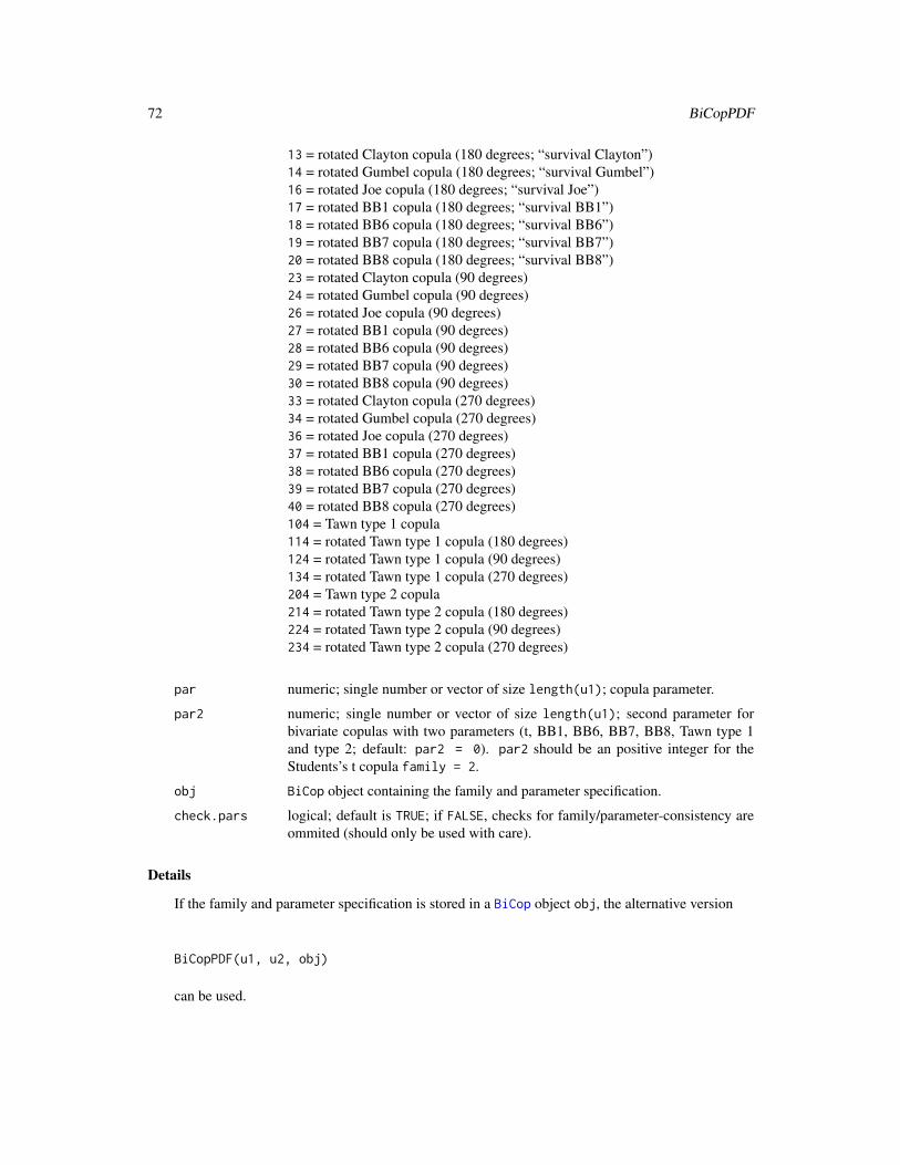
72 BiCopPDF
13 = rotated Clayton copula (180 degrees; “survival Clayton”)14 = rotated Gumbel copula (180 degrees; “survival Gumbel”)16 = rotated Joe copula (180 degrees; “survival Joe”)17 = rotated BB1 copula (180 degrees; “survival BB1”)18 = rotated BB6 copula (180 degrees; “survival BB6”)19 = rotated BB7 copula (180 degrees; “survival BB7”)20 = rotated BB8 copula (180 degrees; “survival BB8”)23 = rotated Clayton copula (90 degrees)24 = rotated Gumbel copula (90 degrees)26 = rotated Joe copula (90 degrees)27 = rotated BB1 copula (90 degrees)28 = rotated BB6 copula (90 degrees)29 = rotated BB7 copula (90 degrees)30 = rotated BB8 copula (90 degrees)33 = rotated Clayton copula (270 degrees)34 = rotated Gumbel copula (270 degrees)36 = rotated Joe copula (270 degrees)37 = rotated BB1 copula (270 degrees)38 = rotated BB6 copula (270 degrees)39 = rotated BB7 copula (270 degrees)40 = rotated BB8 copula (270 degrees)104 = Tawn type 1 copula114 = rotated Tawn type 1 copula (180 degrees)124 = rotated Tawn type 1 copula (90 degrees)134 = rotated Tawn type 1 copula (270 degrees)204 = Tawn type 2 copula214 = rotated Tawn type 2 copula (180 degrees)224 = rotated Tawn type 2 copula (90 degrees)234 = rotated Tawn type 2 copula (270 degrees)
par numeric; single number or vector of size length(u1); copula parameter.
par2 numeric; single number or vector of size length(u1); second parameter forbivariate copulas with two parameters (t, BB1, BB6, BB7, BB8, Tawn type 1and type 2; default: par2 = 0). par2 should be an positive integer for theStudents’s t copula family = 2.
obj BiCop object containing the family and parameter specification.
check.pars logical; default is TRUE; if FALSE, checks for family/parameter-consistency areommited (should only be used with care).
Details
If the family and parameter specification is stored in a BiCop object obj, the alternative version
BiCopPDF(u1, u2, obj)
can be used.
BiCopSelect 73
Value
A numeric vector of the bivariate copula density
• of the copula family
• with parameter(s) par, par2
• evaluated at u1 and u2.
Author(s)
Eike Brechmann
See Also
BiCopCDF, BiCopHfunc, BiCopSim, BiCop
Examples
## simulate from a bivariate Student-t copulacop <- BiCop(family = 2, par = -0.7, par2 = 4)simdata <- BiCopSim(100, cop)
## evaluate the density of the bivariate t-copulau1 <- simdata[,1]u2 <- simdata[,2]BiCopPDF(u1, u2, cop)
## select a bivariate copula for the simulated datafit <- BiCopSelect(u1, u2)summary(fit)## and evaluate its PDFround(BiCopPDF(u1, u2, fit), 3)
BiCopSelect Selection and Maximum Likelihood Estimation of Bivariate CopulaFamilies
Description
This function selects an appropriate bivariate copula family for given bivariate copula data using oneof a range of methods. The corresponding parameter estimates are obtained by maximum likelihoodestimation.
Usage
BiCopSelect(u1, u2, familyset = NA, selectioncrit = "AIC",indeptest = FALSE, level = 0.05, weights = NA, rotations = TRUE,se = FALSE, presel = TRUE, method = "mle")
74 BiCopSelect
Arguments
u1, u2 Data vectors of equal length with values in [0,1].
familyset Vector of bivariate copula families to select from. The vector has to include atleast one bivariate copula family that allows for positive and one that allows fornegative dependence. If familyset = NA (default), selection among all possi-ble families is performed. If a vector of negative numbers is provided, selectionamong all but abs(familyset) families is performed. Coding of bivariate cop-ula families:0 = independence copula1 = Gaussian copula2 = Student t copula (t-copula)3 = Clayton copula4 = Gumbel copula5 = Frank copula6 = Joe copula7 = BB1 copula8 = BB6 copula9 = BB7 copula10 = BB8 copula13 = rotated Clayton copula (180 degrees; “survival Clayton”)14 = rotated Gumbel copula (180 degrees; “survival Gumbel”)16 = rotated Joe copula (180 degrees; “survival Joe”)17 = rotated BB1 copula (180 degrees; “survival BB1”)18 = rotated BB6 copula (180 degrees; “survival BB6”)19 = rotated BB7 copula (180 degrees; “survival BB7”)20 = rotated BB8 copula (180 degrees; “survival BB8”)23 = rotated Clayton copula (90 degrees)24 = rotated Gumbel copula (90 degrees)26 = rotated Joe copula (90 degrees)27 = rotated BB1 copula (90 degrees)28 = rotated BB6 copula (90 degrees)29 = rotated BB7 copula (90 degrees)30 = rotated BB8 copula (90 degrees)33 = rotated Clayton copula (270 degrees)34 = rotated Gumbel copula (270 degrees)36 = rotated Joe copula (270 degrees)37 = rotated BB1 copula (270 degrees)38 = rotated BB6 copula (270 degrees)39 = rotated BB7 copula (270 degrees)40 = rotated BB8 copula (270 degrees)104 = Tawn type 1 copula114 = rotated Tawn type 1 copula (180 degrees)124 = rotated Tawn type 1 copula (90 degrees)134 = rotated Tawn type 1 copula (270 degrees)204 = Tawn type 2 copula214 = rotated Tawn type 2 copula (180 degrees)224 = rotated Tawn type 2 copula (90 degrees)234 = rotated Tawn type 2 copula (270 degrees)
BiCopSelect 75
selectioncrit Character indicating the criterion for bivariate copula selection. Possible choices:selectioncrit = "AIC" (default), "BIC", or "logLik".
indeptest Logical; whether a hypothesis test for the independence of u1 and u2 is per-formed before bivariate copula selection (default: indeptest = FALSE; seeBiCopIndTest). The independence copula is chosen if the null hypothesis ofindependence cannot be rejected.
level Numeric; significance level of the independence test (default: level = 0.05).
weights Numerical; weights for each observation (optional).
rotations If TRUE, all rotations of the families in familyset are included (or substracted).
se Logical; whether standard error(s) of parameter estimates is/are estimated (de-fault: se = FALSE).
presel Logical; whether to exclude families before fitting based on symmetry propertiesof the data. Makes the selection about 30 (on average), but may yield slightlyworse results in few special cases.
method indicates the estimation method: either maximum likelihood estimation (method = "mle";default) or inversion of Kendall’s tau (method = "itau"). For method = "itau"only one parameter families and the Student t copula can be used (family =1,2,3,4,5,6,13,14,16,23,24,26,33,34 or 36). For the t-copula, par2 isfound by a crude profile likelihood optimization over the interval (2, 10].
Details
Copulas can be selected according to the Akaike and Bayesian Information Criteria (AIC and BIC,respectively). First all available copulas are fitted using maximum likelihood estimation. Then thecriteria are computed for all available copula families (e.g., if u1 and u2 are negatively dependent,Clayton, Gumbel, Joe, BB1, BB6, BB7 and BB8 and their survival copulas are not considered) andthe family with the minimum value is chosen. For observations ui,j , i = 1, ..., N, j = 1, 2, theAIC of a bivariate copula family c with parameter(s) θ is defined as
AIC := −2
N∑i=1
ln[c(ui,1, ui,2|θ)] + 2k,
where k = 1 for one parameter copulas and k = 2 for the two parameter t-, BB1, BB6, BB7 andBB8 copulas. Similarly, the BIC is given by
BIC := −2
N∑i=1
ln[c(ui,1, ui,2|θ)] + ln(N)k.
Evidently, if the BIC is chosen, the penalty for two parameter families is stronger than when usingthe AIC.
Additionally a test for independence can be performed beforehand.
76 BiCopSelect
Value
An object of class BiCop, augmented with the following entries:
se, se2 standard errors for the parameter estimates (if se = TRUE,
nobs number of observations,
logLik log likelihood
AIC Aikaike’s Informaton Criterion,
BIC Bayesian’s Informaton Criterion,
emptau empirical value of Kendall’s tau,p.value.indeptest
p-value of the independence test.
Note
For a comprehensive summary of the fitted model, use summary(object); to see all its contents,use str(object).
The parameters of the Student t and BB copulas are restricted (see defaults in BiCopEst to avoidbeing to close to their limiting cases.
Author(s)
Eike Brechmann, Jeffrey Dissmann, Thomas Nagler
References
Akaike, H. (1973). Information theory and an extension of the maximum likelihood principle. In B.N. Petrov and F. Csaki (Eds.), Proceedings of the Second International Symposium on InformationTheory Budapest, Akademiai Kiado, pp. 267-281.
Brechmann, E. C. (2010). Truncated and simplified regular vines and their applications. Diplomathesis, Technische Universitaet Muenchen.http://mediatum.ub.tum.de/?id=1079285.
Manner, H. (2007). Estimation and model selection of copulas with an application to exchangerates. METEOR research memorandum 07/056, Maastricht University.
Schwarz, G. E. (1978). Estimating the dimension of a model. Annals of Statistics 6 (2), 461-464.
See Also
BiCop, BiCopEst, RVineStructureSelect, RVineCopSelect, BiCopIndTest,
Examples
## Example 1: Gaussian copula with large dependence parameterpar <- 0.7fam <- 1dat1 <- BiCopSim(500, fam, par)# select the bivariate copula family and estimate the parameter(s)cop1 <- BiCopSelect(dat1[, 1], dat1[, 2], familyset = 1:10,
BiCopSim 77
indeptest = FALSE, level = 0.05)cop1 # short overviewsummary(cop1) # comprehensive overviewstr(cop1) # see all contents of the object
## Example 2: Gaussian copula with small dependence parameterpar <- 0.01fam <- 1dat2 <- BiCopSim(500, fam, par)# select the bivariate copula family and estimate the parameter(s)cop2 <- BiCopSelect(dat2[, 1], dat2[, 2], familyset = 0:10,
indeptest = TRUE, level = 0.05)summary(cop2)
## Example 3: empirical datadata(daxreturns)cop3 <- BiCopSelect(daxreturns[, 1], daxreturns[, 4], familyset = 0:10)summary(cop3)
BiCopSim Simulation from a Bivariate Copula
Description
This function simulates from a given parametric bivariate copula.
Usage
BiCopSim(N, family, par, par2 = 0, obj = NULL, check.pars = TRUE)
Arguments
N Number of bivariate observations simulated.
family integer; single number or vector of size N; defines the bivariate copula family:0 = independence copula1 = Gaussian copula2 = Student t copula (t-copula)3 = Clayton copula4 = Gumbel copula5 = Frank copula6 = Joe copula7 = BB1 copula8 = BB6 copula9 = BB7 copula10 = BB8 copula13 = rotated Clayton copula (180 degrees; “survival Clayton”)14 = rotated Gumbel copula (180 degrees; “survival Gumbel”)
78 BiCopSim
16 = rotated Joe copula (180 degrees; “survival Joe”)17 = rotated BB1 copula (180 degrees; “survival BB1”)18 = rotated BB6 copula (180 degrees; “survival BB6”)19 = rotated BB7 copula (180 degrees; “survival BB7”)20 = rotated BB8 copula (180 degrees; “survival BB8”)23 = rotated Clayton copula (90 degrees)24 = rotated Gumbel copula (90 degrees)26 = rotated Joe copula (90 degrees)27 = rotated BB1 copula (90 degrees)28 = rotated BB6 copula (90 degrees)29 = rotated BB7 copula (90 degrees)30 = rotated BB8 copula (90 degrees)33 = rotated Clayton copula (270 degrees)34 = rotated Gumbel copula (270 degrees)36 = rotated Joe copula (270 degrees)37 = rotated BB1 copula (270 degrees)38 = rotated BB6 copula (270 degrees)39 = rotated BB7 copula (270 degrees)40 = rotated BB8 copula (270 degrees)104 = Tawn type 1 copula114 = rotated Tawn type 1 copula (180 degrees)124 = rotated Tawn type 1 copula (90 degrees)134 = rotated Tawn type 1 copula (270 degrees)204 = Tawn type 2 copula214 = rotated Tawn type 2 copula (180 degrees)224 = rotated Tawn type 2 copula (90 degrees)234 = rotated Tawn type 2 copula (270 degrees)
par numeric; single number or vector of size N; copula parameter.par2 numeric; single number or vector of size N; second parameter for bivariate cop-
ulas with two parameters (t, BB1, BB6, BB7, BB8, Tawn type 1 and type 2;default: par2 = 0). par2 should be a positive integer for the Students’s t copulafamily = 2.
obj BiCop object containing the family and parameter specification.check.pars logical; default is TRUE; if FALSE, checks for family/parameter-consistency are
ommited (should only be used with care).
Details
If the family and parameter specification is stored in a BiCop object obj, the alternative version
BiCopSim(N, obj)
can be used.
Value
An N x 2 matrix of data simulated from the bivariate copula with family and parameter(s) par,par2.
BiCopTau2Par 79
Author(s)
Ulf Schepsmeier
See Also
BiCop, RVineSim
Examples
# simulate from a bivariate t-copulasimdata <- BiCopSim(100, 2, -0.7, par2 = 4)
# or alternativelyobj <- BiCop(family = 2, par = -0.7, par2 = 4)simdata2 <- BiCopSim(100, obj)
BiCopTau2Par Parameter of a Bivariate Copula for a given Kendall’s Tau Value
Description
This function computes the parameter of a (one parameter) bivariate copula for a given value ofKendall’s tau.
Usage
BiCopTau2Par(family, tau, check.taus = TRUE)
Arguments
family integer; single number or vector of size n; defines the bivariate copula family:0 = independence copula1 = Gaussian copula2 = Student t copula (Here only the first parameter can be computed)3 = Clayton copula4 = Gumbel copula5 = Frank copula6 = Joe copula13 = rotated Clayton copula (180 degrees; “survival Clayton”)14 = rotated Gumbel copula (180 degrees; “survival Gumbel”)16 = rotated Joe copula (180 degrees; “survival Joe”)23 = rotated Clayton copula (90 degrees)24 = rotated Gumbel copula (90 degrees)26 = rotated Joe copula (90 degrees)33 = rotated Clayton copula (270 degrees)34 = rotated Gumbel copula (270 degrees)36 = rotated Joe copula (270 degrees)
80 BiCopTau2Par
Note that (with exception of the t-copula) two parameter bivariate copula fami-lies cannot be used.
tau numeric; single number or vector of size n; Kendall’s tau value (vector withelements in [-1,1]).
check.taus logical; default is TRUE; if FALSE, checks for family/tau-consistency are ommited(should only be used with care).
Value
Parameter (vector) corresponding to the bivariate copula family and the value(s) of Kendall’s tau(τ ).
No. (family) Parameter (par)1, 2 sin(τ π2 )3, 13 2 τ
1−τ4, 14 1
1−τ5 no closed form expression (numerical inversion)6, 16 no closed form expression (numerical inversion)23, 33 2 τ
1+τ
24, 34 − 11+τ
26, 36 no closed form expression (numerical inversion)
Note
The number n can be chosen arbitrarily, but must agree across arguments.
Author(s)
Jakob Stoeber, Eike Brechmann, Tobias Erhardt
References
Joe, H. (1997). Multivariate Models and Dependence Concepts. Chapman and Hall, London.
Czado, C., U. Schepsmeier, and A. Min (2012). Maximum likelihood estimation of mixed C-vineswith application to exchange rates. Statistical Modelling, 12(3), 229-255.
See Also
BiCopPar2Tau
Examples
## Example 1: Gaussian copulatau0 <- 0.5rho <- BiCopTau2Par(family = 1, tau = tau0)BiCop(1, tau = tau0)$par # alternative
## Example 2:vtau <- seq(from = 0.1, to = 0.8, length.out = 100)
BiCopVuongClarke 81
thetaC <- BiCopTau2Par(family = 3, tau = vtau)thetaG <- BiCopTau2Par(family = 4, tau = vtau)thetaF <- BiCopTau2Par(family = 5, tau = vtau)thetaJ <- BiCopTau2Par(family = 6, tau = vtau)plot(thetaC ~ vtau, type = "l", ylim = range(thetaF))lines(thetaG ~ vtau, col = 2)lines(thetaF ~ vtau, col = 3)lines(thetaJ ~ vtau, col = 4)
## Example 3: different copula familiestheta <- BiCopTau2Par(family = c(3,4,6), tau = c(0.4, 0.5, 0.6))BiCopPar2Tau(family = c(3,4,6), par = theta)
BiCopVuongClarke Scoring Goodness-of-Fit Test based on Vuong And Clarke Tests forBivariate Copula Data
Description
Based on the Vuong and Clarke tests this function computes a goodness-of-fit score for each bivari-ate copula family under consideration. For each possible pair of copula families the Vuong and theClarke tests decides which of the two families fits the given data best and assigns a score—pro orcontra a copula family—according to this decision.
Usage
BiCopVuongClarke(u1, u2, familyset = NA, correction = FALSE, level = 0.05,rotations = TRUE)
Arguments
u1, u2 Data vectors of equal length with values in [0,1].
familyset An integer vector of bivariate copula families under consideration, i.e., whichare compared in the goodness-of-fit test. If familyset = NA (default), all pos-sible families are compared. Possible families are:0 = independence copula1 = Gaussian copula2 = Student t copula (t-copula)3 = Clayton copula4 = Gumbel copula5 = Frank copula6 = Joe copula7 = BB1 copula8 = BB6 copula9 = BB7 copula
82 BiCopVuongClarke
10 = BB8 copula13 = rotated Clayton copula (180 degrees; “survival Clayton”)14 = rotated Gumbel copula (180 degrees; “survival Gumbel”)16 = rotated Joe copula (180 degrees; “survival Joe”)17 = rotated BB1 copula (180 degrees; “survival BB1”)18 = rotated BB6 copula (180 degrees; “survival BB6”)19 = rotated BB7 copula (180 degrees; “survival BB7”)20 = rotated BB8 copula (180 degrees; “survival BB8”)23 = rotated Clayton copula (90 degrees)24 = rotated Gumbel copula (90 degrees)26 = rotated Joe copula (90 degrees)27 = rotated BB1 copula (90 degrees)28 = rotated BB6 copula (90 degrees)29 = rotated BB7 copula (90 degrees)30 = rotated BB8 copula (90 degrees)33 = rotated Clayton copula (270 degrees)34 = rotated Gumbel copula (270 degrees)36 = rotated Joe copula (270 degrees)37 = rotated BB1 copula (270 degrees)38 = rotated BB6 copula (270 degrees)39 = rotated BB7 copula (270 degrees)40 = rotated BB8 copula (270 degrees)104 = Tawn type 1 copula114 = rotated Tawn type 1 copula (180 degrees)124 = rotated Tawn type 1 copula (90 degrees)134 = rotated Tawn type 1 copula (270 degrees)204 = Tawn type 2 copula214 = rotated Tawn type 2 copula (180 degrees)224 = rotated Tawn type 2 copula (90 degrees)234 = rotated Tawn type 2 copula (270 degrees)
correction Correction for the number of parameters. Possible choices: correction = FALSE(no correction; default), "Akaike" and "Schwarz".
level Numerical; significance level of the tests (default: level = 0.05).
rotations If TRUE, all rotations of the families in familyset are included (or substracted).
Details
The Vuong as well as the Clarke test compare two models against each other and based on theirnull hypothesis, allow for a statistically significant decision among the two models (see the doc-umentations of RVineVuongTest and RVineClarkeTest for descriptions of the two tests). In thegoodness-of-fit test proposed by Belgorodski (2010) this is used for bivariate copula selection. Itcompares a model 0 to all other possible models under consideration. If model 0 is favored overanother model, a score of "+1" is assigned and similarly a score of "-1" if the other model is de-termined to be superior. No score is assigned, if the respective test cannot discriminate betweentwo models. Both tests can be corrected for the numbers of parameters used in the copulas. Eitherno correction (correction = FALSE), the Akaike correction (correction = "Akaike") or theparsimonious Schwarz correction (correction = "Schwarz") can be used.
BiCopVuongClarke 83
The models compared here are bivariate parametric copulas and we would like to determine whichfamily fits the data better than the other families. E.g., if we would like to test the hypothesis that thebivariate Gaussian copula fits the data best, then we compare the Gaussian copula against all othercopulas under consideration. In doing so, we investigate the null hypothesis "The Gaussian copulafits the data better than all other copulas under consideration", which corresponds to k−1 times thehypothesis "The Gaussian copula Cj fits the data better than copula Ci" for all i = 1, ..., k, i 6= j,where k is the number of bivariate copula families under consideration (length of familyset). Thisprocedure is done not only for one family but for all families under consideration, i.e., two scores,one based on the Vuong and one based on the Clarke test, are returned for each bivariate copulafamily. If used as a goodness-of-fit procedure, the family with the highest score should be selected.
For more and detailed information about the goodness-of-fit test see Belgorodski (2010).
Value
A matrix with Vuong test scores in the first and Clarke test scores in the second row. Column namescorrespond to bivariate copula families (see above).
Author(s)
Ulf Schepsmeier, Eike Brechmann, Natalia Belgorodski
References
Belgorodski, N. (2010) Selecting pair-copula families for regular vines with application to themultivariate analysis of European stock market indices Diploma thesis, Technische UniversitaetMuenchen. http://mediatum.ub.tum.de/?id=1079284.
Clarke, K. A. (2007). A Simple Distribution-Free Test for Nonnested Model Selection. PoliticalAnalysis, 15, 347-363.
Vuong, Q. H. (1989). Ratio tests for model selection and non-nested hypotheses. Econometrica 57(2), 307-333.
See Also
BiCopGofTest, RVineVuongTest, RVineClarkeTest, BiCopSelect
Examples
# simulate from a t-copuladat <- BiCopSim(500, 2, 0.7, 5)
# apply the test for families 1-6BiCopVuongClarke(dat[,1], dat[,2], familyset = 1:6)
84 C2RVine
C2RVine Transform C-Vine to R-Vine Structure
Description
This function transforms a C-vine structure from the package CDVine to the corresponding R-vinestructure.
Usage
C2RVine(order, family, par, par2 = rep(0, length(family)))
Arguments
order A d-dimensional vector specifying the order of the root nodes in the C-vine.
family A d*(d-1)/2 vector of pair-copula families with values0 = independence copula1 = Gaussian copula2 = Student t copula (t-copula)3 = Clayton copula4 = Gumbel copula5 = Frank copula6 = Joe copula7 = BB1 copula8 = BB6 copula9 = BB7 copula10 = BB8 copula13 = rotated Clayton copula (180 degrees; “survival Clayton”)14 = rotated Gumbel copula (180 degrees; “survival Gumbel”)16 = rotated Joe copula (180 degrees; “survival Joe”)17 = rotated BB1 copula (180 degrees; “survival BB1”)18 = rotated BB6 copula (180 degrees; “survival BB6”)19 = rotated BB7 copula (180 degrees; “survival BB7”)20 = rotated BB8 copula (180 degrees; “survival BB8”)23 = rotated Clayton copula (90 degrees)24 = rotated Gumbel copula (90 degrees)26 = rotated Joe copula (90 degrees)27 = rotated BB1 copula (90 degrees)28 = rotated BB6 copula (90 degrees)29 = rotated BB7 copula (90 degrees)30 = rotated BB8 copula (90 degrees)33 = rotated Clayton copula (270 degrees)34 = rotated Gumbel copula (270 degrees)36 = rotated Joe copula (270 degrees)37 = rotated BB1 copula (270 degrees)38 = rotated BB6 copula (270 degrees)39 = rotated BB7 copula (270 degrees)
C2RVine 85
40 = rotated BB8 copula (270 degrees)104 = Tawn type 1 copula114 = rotated Tawn type 1 copula (180 degrees)124 = rotated Tawn type 1 copula (90 degrees)134 = rotated Tawn type 1 copula (270 degrees)204 = Tawn type 2 copula214 = rotated Tawn type 2 copula (180 degrees)224 = rotated Tawn type 2 copula (90 degrees)234 = rotated Tawn type 2 copula (270 degrees)
par A d*(d-1)/2 vector of pair-copula parameters.
par2 A d*(d-1)/2 vector of second pair-copula parameters (optional; default:par2 = rep(0,length(family))), necessary for the t-, BB1, BB6, BB7, BB8,Tawn type 1 and type 2 copulas.
Value
An RVineMatrix object.
Author(s)
Ulf Schepsmeier, Eike Brechmann
See Also
RVineMatrix, D2RVine
Examples
# set up C-vine copula model with mixed pair-copulasd <- 4dd <- d*(d-1)/2order <- 1:dfamily <- c(1, 2, 3, 4, 7, 3)par <- c(0.5, 0.4, 2, 1.5, 1.2, 1.5)par2 <- c(0, 5, 0, 0, 2, 0)
# transform to R-vine matrix notationRVM <- C2RVine(order, family, par, par2)
# load package CDVine for comparisonlibrary(CDVine)
# simulate a sample of size 500 from a 4-dimensional D-vinetype <- 1 # C-vinesimdata <- CDVineSim(500, family, par, par2, type)
# determine log-likelihoodout <- CDVineLogLik(simdata, family, par, par2, type)out$loglik
86 contour.RVineMatrix
# check that log-likelihood stays the sameout2 <- RVineLogLik(simdata, RVM)out2$loglik
contour.RVineMatrix Plotting RVineMatrix objects.
Description
There are two plotting generics for RVineMatrix objects. plot.RVineMatrix plots one or all treesof a given R-vine copula model. Edges can be labeld with information about the correspondingpair-copula. contour.RVineMatrix produces a matrix of contour plots (using plot.BiCop).
Usage
## S3 method for class 'RVineMatrix'contour(x, tree = "ALL", xylim = NULL, cex.nums = 1,data = NULL, ...)
## S3 method for class 'RVineMatrix'plot(x, tree = "ALL", type = 0, edge.labels = NULL,legend.pos = "bottomleft", interactive = FALSE, ...)
Arguments
x RVineMatrix object.
tree "ALL" or integer vector; specifies which trees are plotted.
xylim numeric vector of length 2; sets xlim and ylim for the contours
cex.nums numeric; expansion factor for font of the numbers.
data a data matrix for creating kernel density contours of each pair.
... Arguments passed to plot.network or plot.BiCop respectively.
type integer; specifies how to make use of variable names:0 = variable names are ignored,1 = variable names are used to annotate vertices,2 = uses numbers in plot and adds a legend for variable names.
edge.labels character; either a vector of edge labels or one of the following:"family" = pair-copula family abbreviation (see BiCopName),"par" = pair-copula parameters,"tau" = pair-copula Kendall’s tau (by conversion of parameters)"family-par" = pair-copula family and parameters"family-tau" = pair-copula family and Kendall’s tau.
legend.pos the x argument for legend.
interactive logical; if TRUE, the user is asked to adjust the positioning of vertices with hismouse.
copulaFromFamilyIndex 87
Details
If you want the contour boxes to be perfect squares, the plot height should be 1.25/length(tree)*(d - min(tree))times the plot width.
Author(s)
Thomas Nagler, Nicole Barthel
See Also
RVineMatrix, plot.network, plot.BiCop, BiCopName, legend
Examples
## build vine modelstrucmat <- matrix(c(3, 1, 2, 0, 2, 1, 0, 0, 1), 3, 3)fammat <- matrix(c(0, 1, 6, 0, 0, 3, 0, 0, 0), 3, 3)parmat <- matrix(c(0, 0.3, 3, 0, 0, 1, 0, 0, 0), 3, 3)par2mat <- matrix(c(0, 0, 0, 0, 0, 0, 0, 0, 0), 3, 3)RVM <- RVineMatrix(strucmat, fammat, parmat, par2mat)
# plot trees## Not run: plot(RVM)
# show contour plotscontour(RVM)
copulaFromFamilyIndex Construction of a Copula Object from a VineCopula Family Index
Description
A VineCopula family index along with its parameters is used to construct a corresponding copulaobject.
Usage
copulaFromFamilyIndex(family, par, par2 = 0)
Arguments
family a family index as defined in VineCopula-package
par its first parameter value
par2 if present, its second parameter
88 D2RVine
Value
An object inherting copula corresponding to the specific family.
Author(s)
Benedikt Graeler
Examples
# normalCopula with parameter 0.5copulaFromFamilyIndex(1, 0.5)
# rotated Tawn T2 copula with parameterscopulaFromFamilyIndex(224, -2, 0.5)
D2RVine Transform D-Vine to R-Vine Structure
Description
This function transforms a D-vine structure from the package CDVine to the corresponding R-vinestructure.
Usage
D2RVine(order, family, par, par2 = rep(0, length(family)))
Arguments
order A d-dimensional vector specifying the order of the nodes in the D-vine.
family A d*(d-1)/2 vector of pair-copula families with values0 = independence copula1 = Gaussian copula2 = Student t copula (t-copula)3 = Clayton copula4 = Gumbel copula5 = Frank copula6 = Joe copula7 = BB1 copula8 = BB6 copula9 = BB7 copula10 = BB8 copula13 = rotated Clayton copula (180 degrees; “survival Clayton”)14 = rotated Gumbel copula (180 degrees; “survival Gumbel”)16 = rotated Joe copula (180 degrees; “survival Joe”)
D2RVine 89
17 = rotated BB1 copula (180 degrees; “survival BB1”)18 = rotated BB6 copula (180 degrees; “survival BB6”)19 = rotated BB7 copula (180 degrees; “survival BB7”)20 = rotated BB8 copula (180 degrees; “survival BB8”)23 = rotated Clayton copula (90 degrees)24 = rotated Gumbel copula (90 degrees)26 = rotated Joe copula (90 degrees)27 = rotated BB1 copula (90 degrees)28 = rotated BB6 copula (90 degrees)29 = rotated BB7 copula (90 degrees)30 = rotated BB8 copula (90 degrees)33 = rotated Clayton copula (270 degrees)34 = rotated Gumbel copula (270 degrees)36 = rotated Joe copula (270 degrees)37 = rotated BB1 copula (270 degrees)38 = rotated BB6 copula (270 degrees)39 = rotated BB7 copula (270 degrees)40 = rotated BB8 copula (270 degrees)104 = Tawn type 1 copula114 = rotated Tawn type 1 copula (180 degrees)124 = rotated Tawn type 1 copula (90 degrees)134 = rotated Tawn type 1 copula (270 degrees)204 = Tawn type 2 copula214 = rotated Tawn type 2 copula (180 degrees)224 = rotated Tawn type 2 copula (90 degrees)234 = rotated Tawn type 2 copula (270 degrees)
par A d*(d-1)/2 vector of pair-copula parameters.
par2 A d*(d-1)/2 vector of second pair-copula parameters (optional; default:par2 = rep(0,length(family))), necessary for the t-, BB1, BB6, BB7, BB8,Tawn type 1 and type 2 copulas.
Value
An RVineMatrix object.
Author(s)
Ulf Schepsmeier
See Also
RVineMatrix, C2RVine
Examples
# set up D-vine copula model with mixed pair-copulasd <- 4dd <- d*(d-1)/2
90 daxreturns
order <- 1:dfamily <- c(1, 2, 3, 4, 7, 3)par <- c(0.5, 0.4, 2, 1.5, 1.2, 1.5)par2 <- c(0, 5, 0, 0, 2, 0)
# transform to R-vine matrix notationRVM <- D2RVine(order, family, par, par2)
# load package CDVine for comparisonlibrary(CDVine)
# simulate a sample of size 500 from a 4-dimensional D-vinetype <- 2 # D-vinesimdata <- CDVineSim(500, family, par, par2, type)
# determine log-likelihoodout <- CDVineLogLik(simdata, family, par, par2, type)out$loglik
# check that log-likelihood stays the sameout2 <- RVineLogLik(simdata, RVM)out2$loglik
daxreturns Major German Stocks
Description
This data set contains transformed standardized residuals of daily log returns of 15 major Germanstocks represented in the index DAX observed from January 2005 to August 2009. Each time seriesis filtered using a GARCH(1,1) model with Student t innovations.
Format
A data frame with 1158 observations on 15 variables. Column names correspond to ticker symbolsof the stocks.
Source
Yahoo! Finance
See Also
RVineStructureSelect
ddCopula 91
Examples
# load the data setdata(daxreturns)
# compute the empirical Kendall's tau matrixTauMatrix(daxreturns)
ddCopula Partial Derivatives of Copulas
Description
Similar to dCopula and pCopula the function dduCopula evaluates the partial derivative ∂∂uC(u, v)
and the function ddvCopula evaluates the partial derivative ∂∂vC(u, v) of the provided copula.
Arguments
u Pairs of values for which the partial derivative should be evaluated.
copula The copula object representing the family member of interest.
... additional arguments can be passed on to the underlying functions.
Value
A vector of the evaluated partial derivatives of the same length as rows in u.
Author(s)
Benedikt Graeler
Examples
library(copula)
BB1Cop <- BB1Copula()BB1CopSmpl <- rCopula(100, BB1Cop)
# conditional probabilities of a Gaussian copula given uBB1GivenU <- dduCopula(BB1CopSmpl, BB1Cop)
# vs. conditional probabilities of a Gaussian copula given vBB1GivenV <- ddvCopula(BB1CopSmpl[,c(2,1)], BB1Cop)
plot(BB1GivenU, BB1GivenV)abline(0,1)
92 joeBiCopula
joeBiCopula Constructor of the Joe Family and Rotated Versions thereof
Description
Constructs an object of the (survival surJoeBiCopula, 90 degree rotated r90JoeBiCopula and 270degree rotated r270JoeBiCopula) family for a given parameter. Note that package copula-packageprovides a class joeCopula as well.
Usage
joeBiCopula(param = 2)
Arguments
param The parameter param defines the copula through theta.
Value
One of the respective Joe copula classes (joeBiCopula, surJoeBiCopula, r90JoeBiCopula, r270JoeBiCopula).
Author(s)
Benedikt Graeler
References
Joe, H., (1997). Multivariate Models and Dependence Concepts. Monogra. Stat. Appl. Probab. 73,London: Chapman and Hall.
See Also
See also BB1Copula, BB6Copula, BB7Copula and BB8Copula for further wrapper functions to theVineCopula-package.
Examples
library(copula)
persp(surJoeBiCopula(1.5), dCopula, zlim = c(0,10))persp(r90JoeBiCopula(-1.5), dCopula, zlim = c(0,10))persp(r270JoeBiCopula(-1.5), dCopula, zlim = c(0,10))
joeBiCopula-class 93
joeBiCopula-class Classes "joeBiCopula", "surJoeBiCopula", "r90JoeBiCopula"and "r270JoeBiCopula"
Description
Wrapper classes representing the bivariate Joe, survival Joe, 90 degree and 270 degree rotatedJoe copula families (Joe 1997) from VineCopula-package. Note that package copula-packageprovides a class joeCopula as well.
Objects from the Classes
Objects can be created by calls of the form new("joeBiCopula", ...), new("surJoeBiCopula", ...),new("r90JoeBiCopula", ...) and new("r270JoeBiCopula", ...) or by the functions joeBiCopula,surJoeBiCopula, r90JoeBiCopula and r270JoeBiCopula.
Author(s)
Benedikt Graeler
References
Joe, H., (1997). Multivariate Models and Dependence Concepts. Monogra. Stat. Appl. Probab. 73,London: Chapman and Hall.
See Also
See also BB1Copula, BB6Copula, BB7Copula and BB8Copula for further wrapper classes to theVineCopula-package.
Examples
showClass("surJoeBiCopula")
pairs.copuladata Pairs Plot of Copula Data
Description
This function provides pair plots for copula data. Using default setting it plots bivariate contourplots on the lower panel, scatter plots and correlations on the upper panel and histograms on thediagonal panel.
94 pairs.copuladata
Usage
## S3 method for class 'copuladata'pairs(x, labels = names(x), ...,lower.panel = lp.copuladata, upper.panel = up.copuladata,diag.panel = dp.copuladata, label.pos = 0.85, cex.labels = 1, gap = 0,method = "kendall", ccols = terrain.colors(11), margins = "norm")
Arguments
x copuladata object.
labels variable names/labels.
... other graphical parameters (see par) or options passed to BiCopKDE.
lower.panel panel function to be used on the lower diagonal panels (if not supplied, a defaultfunction is used)
upper.panel panel function to be used on the upper diagonal panels (if not supplied, a defaultfunction is used)
diag.panel panel function to be used on the diagonal panels (if not supplied, a default func-tion is used)
label.pos y position of labels in the diagonal panel; default: label.pos = 0.85.
cex.labels magnification to be used for the labels of the diagonal panel; default: cex.labels = 1.
gap distance between subplots, in margin lines; default: gap = 0.
method a character string indicating which correlation coefficients are computed. Oneof "pearson", "kendall" (default), or "spearman"
ccols colour to be used for the contour plots; default: ccols = terrain.colors(30).
margins character; margins for the contour plots. Options are:"unif" for the original copula density, "norm" for the transformed density withstandard normal margins, "exp" with standard exponential margins, and "flexp"with flipped exponential margins.
Note
If the default panel functions are used
• col changes only the colour of the points in the scatter plot (upper.panel)
• cex changes only the magnification of the points in the scatter plot (upper.panel)
Author(s)
Tobias Erhardt
See Also
pairs, as.copuladata, BiCopKDE
pairs.copuladata 95
Examples
data(daxreturns)
data <- as.copuladata(daxreturns)sel <- c(4,5,14,15)
## pairs plot with default settingspairs(data[sel])
## pairs plot with custom settingsnlevels <- 20pairs(data[sel], cex = 2, pch = 1, col = "black",
diag.panel = NULL, label.pos = 0.5,cex.labels = 2.5, gap = 1,method = "pearson", ccols = heat.colors(nlevels),margins = "flexp")
## pairs plot with own panel functionsup <- function(x, y) {
# upper panel: empirical contour plotop <- par(usr = c(-3, 3, -3, 3), new = TRUE)BiCopKDE(x, y,
levels = c(0.01, 0.05, 0.1, 0.15, 0.2),margins = "exp",axes = FALSE)
on.exit(par(op))}
lp <- function(x, y) {# lower panel: scatter plot (copula data) and correlationop <- par(usr = c(0, 1, 0, 1), new = TRUE)points(x, y, pch = 1, col = "black")r <- cor(x, y, method = "spearman") # Spearman's rhotxt <- format(x = r, digits = 3, nsmall = 3)[1]text(x = 0.5, y = 0.5, labels = txt, cex = 1 + abs(r) * 2, col = "blue")on.exit(par(op))
}
dp <- function(x) {# diagonal panel: histograms (copula data)op <- par(usr = c(0, 1, 0, 1.5), new = TRUE)hist(x, freq = FALSE, add = TRUE, col = "brown", border = "black", main = "")abline(h = 1, col = "black", lty = 2)on.exit(par(op))
}
nlevels <- 20pairs(data[sel],
lower.panel = lp, upper.panel = up, diag.panel = dp, gap = 0.5)
96 plot.BiCop
plot.BiCop Plotting tools for BiCop objects
Description
There are several options for plotting BiCop objects. The density of a bivariate copula density canbe visualized as surface/perspective or contour plot. Optionally, the density can be coupled withstandard normal margins (default for contour plots). Furthermore, a lambda-plot is available (cf.,BiCopLambda).
Usage
## S3 method for class 'BiCop'plot(x, type = "surface", margins, size, ...)
## S3 method for class 'BiCop'contour(x, margins = "norm", size = 100L, ...)
Arguments
x BiCop object.
type plot type; either "surface", "contour", or "lambda" (partial matching is acti-vated); the latter is only implemented for a few families (c.f., BiCopLambda).
margins only relevant for types "contour" and "surface"; options are: "unif" forthe original copula density, "norm" for the transformed density with standardnormal margins, "exp" with standard exponential margins, and "flexp" withflipped exponential margins. Default is "norm" for type = "contour", and"unif" for type = "surface".
size integer; only relevant for types "contour" and "surface"; the plot is based onvalues on a sizexsize grid; default is 100 for type = "contour", and 25 fortype = "surface".
... optional arguments passed to contour or wireframe.
Author(s)
Thomas Nagler
See Also
BiCop, contour, wireframe
pobs 97
Examples
## construct BiCop object for a Tawn copulaobj <- BiCop(family = 104, par = 2.5, par2 = 0.4)
## plotsplot(obj) # surface plot of copula densitycontour(obj) # contour plot with standard normal marginscontour(obj, margins = "unif") # contour plot of copula density
pobs Pseudo-Observations
Description
Compute the pseudo-observations for the given data matrix.
Arguments
x n× d-matrix of random variates to be converted to pseudo-observations.na.last, ties.method
are passed to rank; see there.
lower.tail logical which, if FALSE, returns the pseudo-observations when applying theempirical marginal survival functions.
Details
Given n realizations xi = (xi1, . . . , xid)T , i ∈ {1, . . . , n} of a random vector X , the pseudo-
observations are defined via uij = rij/(n + 1) for i ∈ {1, . . . , n} and j ∈ {1, . . . , d}, where rijdenotes the rank of xij among all xkj , k ∈ {1, . . . , n}. The pseudo-observations can thus also becomputed by component-wise applying the empirical distribution functions to the data and scalingthe result by n/(n + 1). This asymptotically negligible scaling factor is used to force the variatesto fall inside the open unit hypercube, for example, to avoid problems with density evaluation at theboundaries. Note that pobs(, lower.tail=FALSE) simply returns 1-pobs().
Value
matrix of the same dimensions as x containing the pseudo-observations.
Note
This function is borrowed from the copula package.
Author(s)
Marius Hofert
98 RVineAIC
Examples
## Simple definition of the function:pobs
## simulate data from a multivariate normal distributionlibrary(mvtnorm)set.seed(123)Sigma <- matrix(c(2, 1, -0.2, 1, 1, 0.3, -0.2, 0.3, 0.5), 3, 3)mu <- c(-3, 2, 1)dat <- rmvnorm(500, sigma = Sigma)pairs(dat) # plot observations
## compute pseudo-observations for copula inferenceudat <- pobs(dat)pairs(udat)# estimate vine copula modelfit <- RVineStructureSelect(udat, familyset = c(1, 2))
RVineAIC AIC and BIC of an R-Vine Copula Model
Description
These functions calculate the Akaike and Bayesian Information criteria of a d-dimensional R-vinecopula model for a given copula data set.
Usage
RVineAIC(data, RVM, par = RVM$par, par2 = RVM$par2)
RVineBIC(data, RVM, par = RVM$par, par2 = RVM$par2)
Arguments
data An N x d data matrix (with uniform margins).
RVM An RVineMatrix object including the structure and the pair-copula families andparameters.
par A d x d matrix with the pair-copula parameters (optional; default: par = RVM$par).
par2 A d x d matrix with the second parameters of pair-copula families with twoparameters (optional; default: par2 = RVM$par2).
RVineAIC 99
Details
If k denotes the number of parameters of an R-vine copula model with log-likelihood lRV ine andparameter set θ, then the Akaike Information Criterion (AIC) by Akaike (1973) is defined as
AIC := −2lRV ine (θ|u) + 2k,
for observations u = (u′1, ...,u′N )′.
Similarly, the Bayesian Information Criterion (BIC) by Schwarz (1978) is given by
BIC := −2lRV ine (θ|u) + log(N)k.
Value
AIC, BIC The computed AIC or BIC value, respectively.pair.AIC, pair.BIC
A d x d matrix of individual contributions to the AIC or BIC value for each pair-copula, respectively. Note: AIC = sum(pair.AIC) and similarly BIC = sum(pair.BIC).
Author(s)
Eike Brechmann
References
Akaike, H. (1973). Information theory and an extension of the maximum likelihood principle. In B.N. Petrov and F. Csaki (Eds.), Proceedings of the Second International Symposium on InformationTheory Budapest, Akademiai Kiado, pp. 267-281.
Schwarz, G. E. (1978). Estimating the dimension of a model. Annals of Statistics 6 (2), 461-464.
See Also
RVineLogLik, RVineVuongTest, RVineClarkeTest
Examples
# define 5-dimensional R-vine tree structure matrixMatrix <- c(5, 2, 3, 1, 4,
0, 2, 3, 4, 1,0, 0, 3, 4, 1,0, 0, 0, 4, 1,0, 0, 0, 0, 1)
Matrix <- matrix(Matrix, 5, 5)
# define R-vine pair-copula family matrixfamily <- c(0, 1, 3, 4, 4,
0, 0, 3, 4, 1,0, 0, 0, 4, 1,0, 0, 0, 0, 3,0, 0, 0, 0, 0)
100 RVineClarkeTest
family <- matrix(family, 5, 5)
# define R-vine pair-copula parameter matrixpar <- c(0, 0.2, 0.9, 1.5, 3.9,
0, 0, 1.1, 1.6, 0.9,0, 0, 0, 1.9, 0.5,0, 0, 0, 0, 4.8,0, 0, 0, 0, 0)
par <- matrix(par, 5, 5)
# define second R-vine pair-copula parameter matrixpar2 <- matrix(0, 5, 5)
# define RVineMatrix objectRVM <- RVineMatrix(Matrix = Matrix, family = family, par = par, par2 = par2,
names=c("V1", "V2", "V3", "V4", "V5"))
# simulate a sample of size 300 from the R-vine copula modelset.seed(123)simdata <- RVineSim(300,RVM)
# compute AIC and BICRVineAIC(simdata, RVM)RVineBIC(simdata, RVM)
RVineClarkeTest Clarke Test Comparing Two R-Vine Copula Models
Description
This function performs a Clarke test between two d-dimensional R-vine copula models as specifiedby their RVineMatrix objects.
Usage
RVineClarkeTest(data, RVM1, RVM2)
Arguments
data An N x d data matrix (with uniform margins).
RVM1, RVM2 RVineMatrix objects of models 1 and 2.
Details
The test proposed by Clarke (2007) allows to compare non-nested models. For this let c1 and c2 betwo competing vine copulas in terms of their densities and with estimated parameter sets θ1 and θ2.The null hypothesis of statistical indistinguishability of the two models is
RVineClarkeTest 101
H0 : P (mi > 0) = 0.5 ∀i = 1, .., N,
where mi := log[c1(ui|θ1)c2(ui|θ2)
]for observations ui, i = 1, ..., N .
Since under statistical equivalence of the two models the log likelihood ratios of the single obser-vations are uniformly distributed around zero and in expectation 50% of the log likelihood ratiosgreater than zero, the tets statistic
statistic := B =
N∑i=1
1(0,∞)(mi),
where 1 is the indicator function, is distributed Binomial with parameters N and p = 0.5, andcritical values can easily be obtained. Model 1 is interpreted as statistically equivalent to model 2 ifB is not significantly different from the expected value Np = N
2 .
Like AIC and BIC, the Clarke test statistic may be corrected for the number of parameters usedin the models. There are two possible corrections; the Akaike and the Schwarz corrections, whichcorrespond to the penalty terms in the AIC and the BIC, respectively.
Valuestatistic, statistic.Akaike, statistic.Schwarz
Test statistics without correction, with Akaike correction and with Schwarz cor-rection.
p.value, p.value.Akaike, p.value.Schwarz
P-values of tests without correction, with Akaike correction and with Schwarzcorrection.
Author(s)
Jeffrey Dissmann, Eike Brechmann
References
Clarke, K. A. (2007). A Simple Distribution-Free Test for Nonnested Model Selection. PoliticalAnalysis, 15, 347-363.
See Also
RVineVuongTest, RVineAIC, RVineBIC
Examples
# vine structure selection time-consuming (~ 20 sec)
# load data setdata(daxreturns)
# select the R-vine structure, families and parameters
102 RVineCopSelect
RVM <- RVineStructureSelect(daxreturns[,1:5], c(1:6))RVM$MatrixRVM$parRVM$par2
# select the C-vine structure, families and parametersCVM <- RVineStructureSelect(daxreturns[,1:5], c(1:6), type = "CVine")CVM$MatrixCVM$parCVM$par2
# compare the two models based on the dataclarke <- RVineClarkeTest(daxreturns[,1:5], RVM, CVM)clarke$statisticclarke$statistic.Schwarzclarke$p.valueclarke$p.value.Schwarz
RVineCopSelect Sequential Pair-Copula Selection and Estimation for R-Vine CopulaModels
Description
This function fits a R-vine copula model to a d-dimensional copula data set. Pair-copula familiesare selected using BiCopSelect and estimated sequentially.
Usage
RVineCopSelect(data, familyset = NA, Matrix, selectioncrit = "AIC",indeptest = FALSE, level = 0.05, trunclevel = NA, se = FALSE,rotations = TRUE, method = "mle", cores = 1)
Arguments
data N x d data matrix (with uniform margins).
familyset integer vector of pair-copula families to select from. The vector has to includeat least one pair-copula family that allows for positive and one that allows fornegative dependence. Not listed copula families might be included to betterhandle limit cases. If familyset = NA (default), selection among all possiblefamilies is performed. If a vector of negative numbers is provided, selectionamong all but abs(familyset) is performed. Coding of pair copula families isthe same as in BiCop.
Matrix lower or upper triangular d x d matrix that defines the R-vine tree structure.
selectioncrit Character indicating the criterion for pair-copula selection. Possible choices:selectioncrit = "AIC" (default), "BIC", or "logLik" (see BiCopSelect).
RVineCopSelect 103
indeptest Logical; whether a hypothesis test for the independence of u1 and u2 is per-formed before bivariate copula selection (default: indeptest = FALSE; seeBiCopIndTest). The independence copula is chosen for a (conditional) pair ifthe null hypothesis of independence cannot be rejected.
level numeric; significance level of the independence test (default: level = 0.05).
trunclevel integer; level of truncation.
se Logical; whether standard errors are estimated (default: se = FALSE).
rotations logical; if TRUE, all rotations of the families in familyset are included.
method indicates the estimation method: either maximum likelihood estimation (method = "mle";default) or inversion of Kendall’s tau (method = "itau"). For method = "itau"only one parameter families and the Student t copula can be used (family =1,2,3,4,5,6,13,14,16,23,24,26,33,34 or 36). For the t-copula, par2 isfound by a crude profile likelihood optimization over the interval (2, 10].
cores integer; if cores > 1, estimation will be parallized within each tree (usingforeach). Note that parallelization causes substantial overhead and may beslower than single-threaded computation when dimension, sample size, or fam-ilyset are small or method = "itau".
Details
R-vine copula models with unknown structure can be specified using RVineStructureSelect.
Value
An RVineMatrix object with the selected families (RVM$family) as well as sequentially estimatedparameters stored in RVM$par and RVM$par2. The object is augmented by the following informationabout the fit:
se, se2 standard errors for the parameter estimates (if se = TRUE; note that these areonly approximate since they do not account for the sequential nature of the esti-mation,
nobs number of observations,logLik, pair.logLik
log likelihood (overall and pairwise)
AIC, pair.AIC Aikaike’s Informaton Criterion (overall and pairwise),
BIC, pair.BIC Bayesian’s Informaton Criterion (overall and pairwise),
emptau matrix of empirical values of Kendall’s tau,p.value.indeptest
matrix of p-values of the independence test.
#’
Note
For a comprehensive summary of the vine copula model, use summary(object); to see all itscontents, use str(object).
104 RVineCopSelect
Author(s)
Eike Brechmann, Thomas Nagler
References
Brechmann, E. C., C. Czado, and K. Aas (2012). Truncated regular vines in high dimensions withapplications to financial data. Canadian Journal of Statistics 40 (1), 68-85.
Dissmann, J. F., E. C. Brechmann, C. Czado, and D. Kurowicka (2013). Selecting and estimatingregular vine copulae and application to financial returns. Computational Statistics & Data Analysis,59 (1), 52-69.
See Also
RVineMatrix, BiCop, BiCopSelect, plot.RVineMatrix, contour.RVineMatrix, foreach
Examples
# define 5-dimensional R-vine tree structure matrixMatrix <- c(5, 2, 3, 1, 4,
0, 2, 3, 4, 1,0, 0, 3, 4, 1,0, 0, 0, 4, 1,0, 0, 0, 0, 1)
Matrix <- matrix(Matrix, 5, 5)# define R-vine pair-copula family matrixfamily <- c(0, 1, 3, 4, 4,
0, 0, 3, 4, 1,0, 0, 0, 4, 1,0, 0, 0, 0, 3,0, 0, 0, 0, 0)
family <- matrix(family, 5, 5)# define R-vine pair-copula parameter matrixpar <- c(0, 0.2, 0.9, 1.5, 3.9,
0, 0, 1.1, 1.6, 0.9,0, 0, 0, 1.9, 0.5,0, 0, 0, 0, 4.8,0, 0, 0, 0, 0)
par <- matrix(par, 5, 5)# define second R-vine pair-copula parameter matrixpar2 <- matrix(0, 5, 5)
## define RVineMatrix objectRVM <- RVineMatrix(Matrix = Matrix, family = family,
par = par, par2 = par2,names = c("V1", "V2", "V3", "V4", "V5"))
## simulate a sample of size 500 from the R-vine copula modelset.seed(123)simdata <- RVineSim(500, RVM)
RVineCor2pcor 105
## determine the pair-copula families and parametersRVM1 <- RVineCopSelect(simdata, familyset = c(1, 3, 4, 5 ,6), Matrix)
## see the object's content or a summarystr(RVM1)summary(RVM1)
## inspect the fitted model using plots## Not run: plot(RVM1) # tree structure
contour(RVM1) # contour plots of all pair-copulas
RVineCor2pcor (Partial) Correlations for R-Vine Copula Models
Description
Correlations to partial correlations and vice versa for R-vines with independence, Gaussian andt-copulas.
Usage
RVineCor2pcor(RVM, corMat)
RVinePcor2cor(RVM)
Arguments
RVM RVineMatrix defining only the R-vine structure for Cor2pcor and providing aswell the partial correlations for Pcor2cor.
corMat correlation matrix
Value
RVM RVineMatrix with transformed partial correlations (for Cor2pcor)
cor correlation matrix (for Pcor2cor)
Note
The behavior of RVinePcor2ccor differs from older versions (<= 1.4). The RVM object is nownormalized such that the order of the returned correlation matrix conforms with the correlationmatrix of the data. If RVM$names are non-default, the initial ordering of the variables cannot betraced back and the matrix has to be interpreted as inidicated by the row- and column names.
106 RVineGofTest
Examples
## create RVineMatrix-object for Gaussian vineMatrix <- matrix(c(1, 3, 4, 2,
0, 3, 4, 2,0, 0, 4, 2,0, 0, 0, 2), 4, 4)
family <- matrix(c(0, 1, 1, 1,0, 0, 1, 1,0, 0, 0, 1,0, 0, 0, 0), 4, 4)
par <- matrix(c(0, 0.2, 0, 0.6,0, 0, 0.2, 0.6,0, 0, 0, 0.6,0, 0, 0, 0), 4, 4)
RVM <- RVineMatrix(Matrix, family, par)
## calculate correlation matrix corresponding to the R-Vine modelnewcor <- RVinePcor2cor(RVM)
## transform back to partial correlationsRVineCor2pcor(RVM, newcor)$par
## check if they are equalall.equal(RVM$par, RVineCor2pcor(RVM, newcor)$par)
RVineGofTest Goodness-of-Fit Tests for R-Vine Copula Models
Description
This function performs a goodness-of-fit test for R-vine copula models. There are 15 differentgoodness-of-fit tests implemented, described in Schepsmeier (2013).
Usage
RVineGofTest(data, RVM, method = "White", statistic = "CvM", B = 200,alpha = 2)
Arguments
data An N x d data matrix (with uniform margins).
RVM RVineMatrix objects of the R-vine model under the null hypothesis.Only the following copula families are allowed in RVM$family due to restric-tions in RVineGrad and RVineHessian0 = independence copula1 = Gaussian copula
RVineGofTest 107
2 = Student t copula (t-copula)3 = Clayton copula4 = Gumbel copula5 = Frank copula6 = Joe copula13 = rotated Clayton copula (180 degrees; “survival Clayton”)14 = rotated Gumbel copula (180 degrees; “survival Gumbel”)16 = rotated Joe copula (180 degrees; “survival Joe”)23 = rotated Clayton copula (90 degrees)24 = rotated Gumbel copula (90 degrees)26 = rotated Joe copula (90 degrees)33 = rotated Clayton copula (270 degrees)34 = rotated Gumbel copula (270 degrees)36 = rotated Joe copula (270 degrees)
method A string indicating the goodness-of-fit method:"White" = goodness-of-fit test based on White’s information matrix equality(default)"IR" = goodness-of-fit test based on the information ratio"Breymann" = goodness-of-fit test based on the probability integral transform(PIT) and the aggregation to univariate data by Breymann et al. (2003)."Berg" = goodness-of-fit test based on the probability integral transform (PIT)and the aggregation to univariate data by Berg and Bakken (2007)."Berg2" = second goodness-of-fit test based on the probability integral trans-form (PIT) and the aggregation to univariate data by Berg and Bakken (2007)."ECP" = goodness-of-fit test based on the empirical copula process (ECP)"ECP2" = goodness-of-fit test based on the combination of probability integraltransform (PIT) and empirical copula process (ECP) (Genest et al. 2009)
statistic A string indicating the goodness-of-fit test statistic type:"CvM" = Cramer-von Mises test statistic (univariate for "Breymann", "Berg"and "Berg2", multivariate for "ECP" and "ECP2")"KS" = Kolmogorov-Smirnov test statistic (univariate for "Breymann", "Berg"and "Berg2", multivariate for "ECP" and "ECP2")"AD" = Anderson-Darling test statistic (only univariate for "Breymann", "Berg"and "Berg2")
B an integer for the number of bootstrap steps (default B = 200)For B = 0 the asymptotic p-value is returned if available, otherwise only the teststatistic is returned.WARNING: If B is chosen too large, computations will take very long.
alpha an integer of the set 2,4,6,... for the "Berg2" goodness-of-fit test (defaultalpha = 2)
Details
method = "White":This goodness-of fit test uses the information matrix equality of White (1982) and was original in-vestigated by Huang and Prokhorov (2011) for copulas.
108 RVineGofTest
Schepsmeier (2012) enhanced their approach to the vine copula case.The main contribution is that under correct model specification the Fisher Information can be equiv-alently calculated as minus the expected Hessian matrix or as the expected outer product of the scorefunction. The null hypothesis is
H0 : H(θ) +C(θ) = 0
against the alternativeH1 : H(θ) +C(θ) 6= 0,
where H(θ) is the expected Hessian matrix and C(θ) is the expected outer product of the scorefunction.For the calculation of the test statistic we use the consistent maximum likelihood estimator θ andthe sample counter parts ofH(θ) and C(θ).The correction of the Covariance-Matrix in the test statistic for the uncertainty in the margins isskipped. The implemented test assumes that there is no uncertainty in the margins. The correctioncan be found in Huang and Prokhorov (2011) for bivariate copulas and in Schepsmeier (2013) forvine copulas. It involves multi-dimensional integrals.
method = "IR":As the White test the information matrix ratio test is based on the expected Hessian matrix H(θ)and the expected outer product of the score function C(θ).
H0 : −H(θ)−1C(θ) = Ip
against the alternativeH1 : −H(θ)−1C(θ) 6= Ip.
The test statistic can then be calculated as
IRn := tr(Φ(θ))/p
with Φ(θ) = −H(θ)−1C(θ), p is the number of parameters, i.e. the length of θ, and tr(A) is thetrace of the matrix AFor details see Schepsmeier (2013)
method = "Breymann", method = "Berg" and method = "Berg2":These tests are based on the multivariate probability integral transform (PIT) applied in RVinePIT.The multivariate data yi returned form the PIT are aggregated to univariate data by different aggre-gation functions Γ(·) in the sum
st =
d∑i=1
Γ(yit), t = 1, ..., n
. In Breymann et al. (2003) the weight function is suggested as Γ(·) = Φ−1(·)2, while in Bergand Bakken (2007) the weight function is either Γ(·) = | · −0.5| (method="Berg") or Γ(·) =(· − 0.5)α, α = 2, 4, 6, ... (method="Berg2").Furthermore, the "Berg" and "Berg2" test are based on the order statistics of the PIT returns.See Berg and Bakken (2007) or Schepsmeier (2013) for details.
RVineGofTest 109
method = "ECP" and method = "ECP2":Both tests are test for H0 : C ∈ C0 against H1 : C /∈ C0 where C denotes the (vine) copula dis-tribution function and C0 is a class of parametric (vine) copulas with Θ ⊆ Rp being the parameterspace of dimension p. They are based on the empirical copula process (ECP)
Cn(u)− Cθn(u),
with u = (u1, . . . , ud) ∈ [0, 1]d and Cn(u) = 1n+1
∑nt=1 1{Ut1≤u1,...,Utd≤ud}. The ECP is utilized
in a multivariate Cramer-von Mises (CvM) or multivariate Kolmogorov-Smirnov (KS) based teststatistic. An extension of the ECP-test is the combination of the multivariate PIT approach with theECP. The general idea is that the transformed data of a multivariate PIT should be "close" to theindependence copula Genest et al. (2009). Thus a distance of CvM or KS type between them isconsidered. This approach is called ECP2. Again we refer to Schepsmeier (2013) for details.
Value
For method = "White":
White test statistic
p.value p-value, either asymptotic for B = 0 or bootstrapped for B > 0
For method = "IR":
IR test statistic (raw version as stated above)
p.value So far no p-value is returned nigher a asymptotic nor a bootstrapped one. How tocalculated a bootstrapped p-value is explained in Schepsmeier (2013). Be aware,that the test statistics than have to be adjusted with the empirical variance.
For method = "Breymann", method = "Berg" and method = "Berg2":
CvM, KS, AD test statistic according to the choice of statistic
p.value p-value, either asymptotic for B = 0 or bootstrapped for B > 0. A asymptoticp-value is only available for the Anderson-Darling test statistic if the R-packageADGofTest is loaded.Furthermore, a asymptotic p-value can be calculated for the Kolmogorov-Smirnovtest statistic. For the Cramer-von Mises no asymptotic p-value is available so far.
For method = "ECP" and method = "ECP2":
CvM, KS test statistic according to the choice of statistic
p.value bootstrapped p-value
Warning: The code for all the p-values are not yet approved since some of them are moved fromR-code to C-code. If you need p-values the best way is to write your own algorithm as suggested inSchepsmeier (2013) to get bootstrapped p-values.
Author(s)
Ulf Schepsmeier
110 RVineGrad
References
Berg, D. and H. Bakken (2007) A copula goodness-of-fit apprach based on the conditional proba-bility integral transformation. http://www.danielberg.no/publications/Btest.pdf
Breymann, W., A. Dias and P. Embrechts (2003) Dependence structures for multivariate high-frequence data in finance. Quantitative Finance 3, 1-14
Genest, C., B. Remillard, and D. Beaudoin (2009) Goodness-of-fit tests for copulas: a review andpower study. Insur. Math. Econ. 44, 199-213.
Huang, w. and A. Prokhorov (2011). A goodness-of-fit test for copulas. to appear in EconometricReviews
Schepsmeier, U. (2013) A goodness-of-fit test for regular vine copula models. Preprint http://arxiv.org/abs/1306.0818
Schepsmeier, U. (2015) Efficient information based goodness-of-fit tests for vine copula modelswith fixed margins. Journal of Multivariate Analysis 138, 34-52.
White, H. (1982) Maximum likelihood estimation of misspecified models, Econometrica, 50, 1-26.
See Also
BiCopGofTest, RVinePIT
Examples
## time-consuming example
# load data setdata(daxreturns)
# select the R-vine structure, families and parametersRVM <- RVineStructureSelect(daxreturns[,1:5], c(1:6))
# White test with asymptotic p-valueRVineGofTest(daxreturns[,1:5], RVM, B = 0)
# ECP2 test with Cramer-von-Mises test statistic and a bootstrap# with 200 replications for the calculation of the p-valueRVineGofTest(daxreturns[,1:5], RVM, method = "ECP2",
statistic = "CvM", B = 200)
RVineGrad Gradient of the Log-Likelihood of an R-Vine Copula Model
Description
This function calculates the gradient of the log-likelihood of a d-dimensional R-vine copula modelwith respect to the copula parameter and evaluates it on a given copula data set.
RVineGrad 111
Usage
RVineGrad(data, RVM, par = RVM$par, par2 = RVM$par2, start.V = NA,posParams = (RVM$family > 0))
Arguments
data An N x d data matrix (with uniform margins).RVM An RVineMatrix object including the structure and the pair-copula families and
parameters.Only the following copula families are allowed in RVM$family0 = independence copula1 = Gaussian copula2 = Student t copula (t-copula)3 = Clayton copula4 = Gumbel copula5 = Frank copula6 = Joe copula13 = rotated Clayton copula (180 degrees; “survival Clayton”)14 = rotated Gumbel copula (180 degrees; “survival Gumbel”)16 = rotated Joe copula (180 degrees; “survival Joe”)23 = rotated Clayton copula (90 degrees)24 = rotated Gumbel copula (90 degrees)26 = rotated Joe copula (90 degrees)33 = rotated Clayton copula (270 degrees)34 = rotated Gumbel copula (270 degrees)36 = rotated Joe copula (270 degrees)
par A d x d matrix with the pair-copula parameters (optional; default: par = RVM$par).par2 A d x d matrix with the second parameters of pair-copula families with two
parameters (optional; default: par2 = RVM$par2).start.V Transformations (h-functions and log-likelihoods of each pair-copula) of previ-
ous calculations (see output; default: start.V = NA).posParams A d x d matrix indicating which copula has to be considered in the gradient
(default: posParams = (RVM$family > 0)).
Details
The ordering of the gradient is due to the ordering of the R-vine matrix. The gradient starts at thelower right corner of the R-vine matrix and goes column by column to the left and up, i.e. the firstentry of the gradient is the last entry of the second last column of the par-matrix followed by thelast entry of the third last column and the second last entry of this column. If there is a copulafamily with two parameters, i.e. the t-copula, the derivative with respect to the second parameter isat the end of the gradient vector in order of their occurrence.
Value
gradient The calculated gradient of the log-likelihood value of the R-vine copula model. (threematrices: direct, indirect and value).
112 RVineGrad
Note
The gradient for R-vine copula models with two parameter Archimedean copulas, i.e. BB1, BB6,BB7, BB8 and their rotated versions can not yet be calculated. The derivatives of these bivariatecopulas are more complicated.
Author(s)
Ulf Schepsmeier, Jakob Stoeber
References
Dissmann, J. F., E. C. Brechmann, C. Czado, and D. Kurowicka (2013). Selecting and estimatingregular vine copulae and application to financial returns. Computational Statistics & Data Analysis,59 (1), 52-69.
Schepsmeier, U. and J. Stoeber (2014) Derivatives and Fisher information of bivariate copulas.Statistical Papers, 55(2), 525-542. online first: http://link.springer.com/article/10.1007/s00362-013-0498-x.
Web supplement: Derivatives and Fisher Information of bivariate copulas. http://mediatum.ub.tum.de/node?id=1119201
Stoeber, J. and U. Schepsmeier (2013). Estimating standard errors in regular vine copula models.Computational Statistics, 28 (6), 2679-2707 http://link.springer.com/article/10.1007/s00180-013-0423-8#.
See Also
BiCopDeriv, BiCopDeriv2, BiCopHfuncDeriv, BiCopHfuncDeriv2,RVineMatrix, RVineMLE, RVineHessian
Examples
# define 5-dimensional R-vine tree structure matrixMatrix <- c(5, 2, 3, 1, 4,
0, 2, 3, 4, 1,0, 0, 3, 4, 1,0, 0, 0, 4, 1,0, 0, 0, 0, 1)
Matrix <- matrix(Matrix, 5, 5)
# define R-vine pair-copula family matrixfamily <- c(0, 1, 3, 4, 4,
0, 0, 3, 4, 1,0, 0, 0, 4, 1,0, 0, 0, 0, 3,0, 0, 0, 0, 0)
family <- matrix(family, 5, 5)
# define R-vine pair-copula parameter matrixpar <- c(0, 0.2, 0.9, 1.5, 3.9,
0, 0, 1.1, 1.6, 0.9,0, 0, 0, 1.9, 0.5,
RVineHessian 113
0, 0, 0, 0, 4.8,0, 0, 0, 0, 0)
par <- matrix(par, 5, 5)
# define second R-vine pair-copula parameter matrixpar2 <- matrix(0, 5, 5)
# define RVineMatrix objectRVM <- RVineMatrix(Matrix = Matrix, family = family,
par = par, par2 = par2,names = c("V1", "V2", "V3", "V4", "V5"))
# simulate a sample of size 300 from the R-vine copula modelset.seed(123)simdata <- RVineSim(300, RVM)
# compute the gradient of the first row of the dataout2 <- RVineGrad(simdata[1,], RVM)out2$gradient
RVineHessian Hessian Matrix of the Log-Likelihood of an R-Vine Copula Model
Description
This function calculates the Hessian matrix of the log-likelihood of a d-dimensional R-vine copulamodel with respect to the copula parameter and evaluates it on a given copula data set.
Usage
RVineHessian(data, RVM)
Arguments
data An N x d data matrix (with uniform margins).
RVM An RVineMatrix object including the structure, the pair-copula families, andthe parameters.Only the following copula families are allowed in RVM$family0 = independence copula1 = Gaussian copula2 = Student t copula (t-copula)3 = Clayton copula4 = Gumbel copula5 = Frank copula6 = Joe copula13 = rotated Clayton copula (180 degrees; “survival Clayton”)14 = rotated Gumbel copula (180 degrees; “survival Gumbel”)
114 RVineHessian
16 = rotated Joe copula (180 degrees; “survival Joe”)23 = rotated Clayton copula (90 degrees)24 = rotated Gumbel copula (90 degrees)26 = rotated Joe copula (90 degrees)33 = rotated Clayton copula (270 degrees)34 = rotated Gumbel copula (270 degrees)36 = rotated Joe copula (270 degrees)
Value
hessian The calculated Hessian matrix of the log-likelihood value of the R-vine copulamodel.
der The product of the gradient vector with its transposed version.
Note
The Hessian matrix is not available for R-vine copula models with two parameter Archimedeancopulas, i.e. BB1, BB6, BB7, BB8 and their rotated versions.
Author(s)
Ulf Schepsmeier, Jakob Stoeber
References
Dissmann, J. F., E. C. Brechmann, C. Czado, and D. Kurowicka (2013). Selecting and estimatingregular vine copulae and application to financial returns. Computational Statistics & Data Analysis,59 (1), 52-69.
Schepsmeier, U. and J. Stoeber (2014) Derivatives and Fisher information of bivariate copulas.Statistical Papers, 55(2), 525-542. online first: http://link.springer.com/article/10.1007/s00362-013-0498-x.
Web supplement: Derivatives and Fisher Information of bivariate copulas. http://mediatum.ub.tum.de/node?id=1119201
Stoeber, J. and U. Schepsmeier (2013). Estimating standard errors in regular vine copula models.Computational Statistics, 28 (6), 2679-2707 http://link.springer.com/article/10.1007/s00180-013-0423-8#.
See Also
BiCopDeriv, BiCopDeriv2, BiCopHfuncDeriv, BiCopHfuncDeriv2,RVineMatrix, RVineMLE, RVineGrad
Examples
# define 5-dimensional R-vine tree structure matrixMatrix <- c(5, 2, 3, 1, 4,
0, 2, 3, 4, 1,0, 0, 3, 4, 1,
RVineLogLik 115
0, 0, 0, 4, 1,0, 0, 0, 0, 1)
Matrix <- matrix(Matrix, 5, 5)
# define R-vine pair-copula family matrixfamily <- c(0, 1, 3, 4, 4,
0, 0, 3, 4, 1,0, 0, 0, 4, 1,0, 0, 0, 0, 3,0, 0, 0, 0, 0)
family <- matrix(family, 5, 5)
# define R-vine pair-copula parameter matrixpar <- c(0, 0.2, 0.9, 1.5, 3.9,
0, 0, 1.1, 1.6, 0.9,0, 0, 0, 1.9, 0.5,0, 0, 0, 0, 4.8,0, 0, 0, 0, 0)
par <- matrix(par, 5, 5)
# define second R-vine pair-copula parameter matrixpar2 <- matrix(0, 5, 5)
# define RVineMatrix objectRVM <- RVineMatrix(Matrix = Matrix, family = family,
par = par, par2 = par2,names = c("V1", "V2", "V3", "V4", "V5"))
# simulate a sample of size 300 from the R-vine copula modelset.seed(123)simdata <- RVineSim(300, RVM)
# compute the Hessian matrix of the first row of the dataout2 <- RVineHessian(simdata[1,], RVM)out2$hessian
RVineLogLik Log-Likelihood of an R-Vine Copula Model
Description
This function calculates the log-likelihood of a d-dimensional R-vine copula model for a givencopula data set.
Usage
RVineLogLik(data, RVM, par = RVM$par, par2 = RVM$par2, separate = FALSE,verbose = TRUE, check.pars = TRUE, calculate.V = TRUE)
116 RVineLogLik
Arguments
data An N x d data matrix (with uniform margins).
RVM An RVineMatrix object including the structure and the pair-copula families andparameters.
par A d x d matrix with the pair-copula parameters (optional; default: par = RVM$par).
par2 A d x d matrix with the second parameters of pair-copula families with twoparameters (optional; default: par2 = RVM$par2).
separate Logical; whether log-likelihoods are returned point wisely (default: separate = FALSE).
verbose In case something goes wrong, additional output will be plotted.
check.pars logical; default is TRUE; if FALSE, checks for family/parameter-consistency areommited (should only be used with care).
calculate.V logical; whether V matrices should be calculated. Default is TRUE, but requiresa lot of memory when dimension is large. Use FALSE for a memory efficientversion.
Details
For observations u = (u′1, ...,u′N )′ the log-likelihood of a d-dimensional R-vine copula with d− 1
trees and corresponding edge sets E1, ..., Ed−1 is given by
loglik := lRV ine (θ|u)
=
N∑i=1
d−1∑`=1
∑e∈E`
ln[cj(e),k(e)|D(e)(F (ui,j(e)|ui,D(e)), F (ui,k(e)|ui,D(e))|θj(e),k(e)|D(e))]
where ui = (ui,1, ..., ui,d)′ ∈ [0, 1]d, i = 1, ..., N . Further cj(e),k(e)|D(e) denotes a bivariate cop-
ula density associated to an edge e and with parameter(s) θj(e),k(e)|D(e). Conditional distributionfunctions such as F (ui,j(e)|ui,D(e)) are obtained recursively using the relationship
h(u|v,θ) := F (u|v) = dCuvj |v−j(F (u|v−j), F (vj |v−j))/dF (vj |v−j),
where Cuvj |v−jis a bivariate copula distribution function with parameter(s) θ and v−j denotes a
vector with the j-th component vj removed. The notation of h-functions is introduced for conve-nience. For more details see Dissmann et al. (2013).
Value
loglik The calculated log-likelihood value of the R-vine copula model.
V The stored transformations (h-functions and log-likelihoods of each pair-copula)which may be used for posterior updates (three matrices: direct, indirect andvalue).
Author(s)
Ulf Schepsmeier, Jeffrey Dissmann, Jakob Stoeber
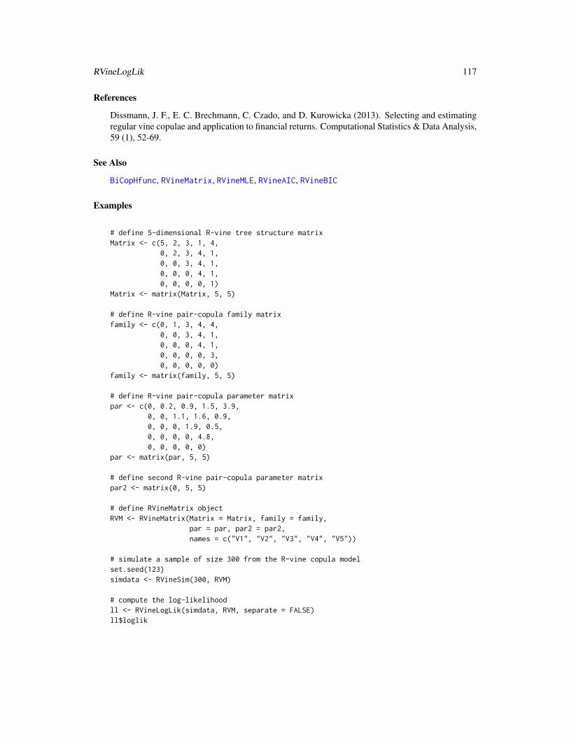
RVineLogLik 117
References
Dissmann, J. F., E. C. Brechmann, C. Czado, and D. Kurowicka (2013). Selecting and estimatingregular vine copulae and application to financial returns. Computational Statistics & Data Analysis,59 (1), 52-69.
See Also
BiCopHfunc, RVineMatrix, RVineMLE, RVineAIC, RVineBIC
Examples
# define 5-dimensional R-vine tree structure matrixMatrix <- c(5, 2, 3, 1, 4,
0, 2, 3, 4, 1,0, 0, 3, 4, 1,0, 0, 0, 4, 1,0, 0, 0, 0, 1)
Matrix <- matrix(Matrix, 5, 5)
# define R-vine pair-copula family matrixfamily <- c(0, 1, 3, 4, 4,
0, 0, 3, 4, 1,0, 0, 0, 4, 1,0, 0, 0, 0, 3,0, 0, 0, 0, 0)
family <- matrix(family, 5, 5)
# define R-vine pair-copula parameter matrixpar <- c(0, 0.2, 0.9, 1.5, 3.9,
0, 0, 1.1, 1.6, 0.9,0, 0, 0, 1.9, 0.5,0, 0, 0, 0, 4.8,0, 0, 0, 0, 0)
par <- matrix(par, 5, 5)
# define second R-vine pair-copula parameter matrixpar2 <- matrix(0, 5, 5)
# define RVineMatrix objectRVM <- RVineMatrix(Matrix = Matrix, family = family,
par = par, par2 = par2,names = c("V1", "V2", "V3", "V4", "V5"))
# simulate a sample of size 300 from the R-vine copula modelset.seed(123)simdata <- RVineSim(300, RVM)
# compute the log-likelihoodll <- RVineLogLik(simdata, RVM, separate = FALSE)ll$loglik
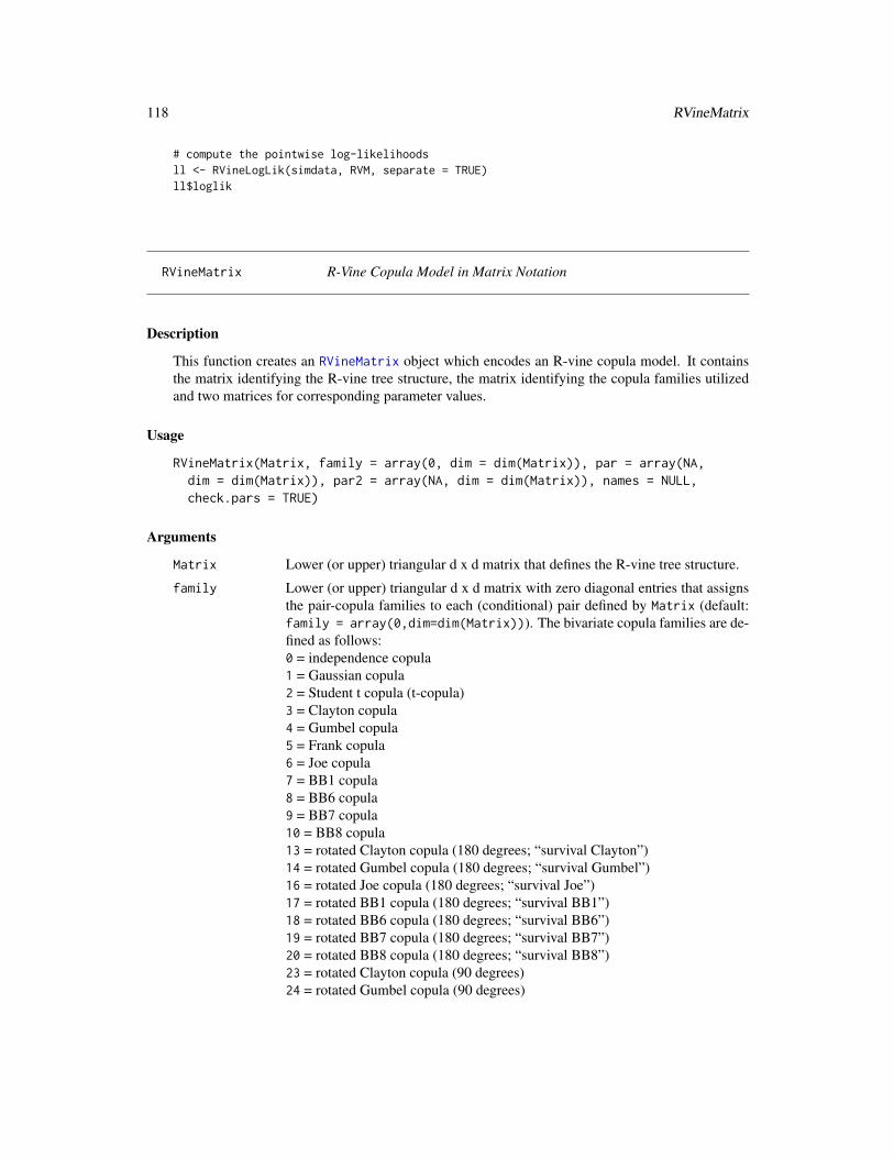
118 RVineMatrix
# compute the pointwise log-likelihoodsll <- RVineLogLik(simdata, RVM, separate = TRUE)ll$loglik
RVineMatrix R-Vine Copula Model in Matrix Notation
Description
This function creates an RVineMatrix object which encodes an R-vine copula model. It containsthe matrix identifying the R-vine tree structure, the matrix identifying the copula families utilizedand two matrices for corresponding parameter values.
Usage
RVineMatrix(Matrix, family = array(0, dim = dim(Matrix)), par = array(NA,dim = dim(Matrix)), par2 = array(NA, dim = dim(Matrix)), names = NULL,check.pars = TRUE)
Arguments
Matrix Lower (or upper) triangular d x d matrix that defines the R-vine tree structure.
family Lower (or upper) triangular d x d matrix with zero diagonal entries that assignsthe pair-copula families to each (conditional) pair defined by Matrix (default:family = array(0,dim=dim(Matrix))). The bivariate copula families are de-fined as follows:0 = independence copula1 = Gaussian copula2 = Student t copula (t-copula)3 = Clayton copula4 = Gumbel copula5 = Frank copula6 = Joe copula7 = BB1 copula8 = BB6 copula9 = BB7 copula10 = BB8 copula13 = rotated Clayton copula (180 degrees; “survival Clayton”)14 = rotated Gumbel copula (180 degrees; “survival Gumbel”)16 = rotated Joe copula (180 degrees; “survival Joe”)17 = rotated BB1 copula (180 degrees; “survival BB1”)18 = rotated BB6 copula (180 degrees; “survival BB6”)19 = rotated BB7 copula (180 degrees; “survival BB7”)20 = rotated BB8 copula (180 degrees; “survival BB8”)23 = rotated Clayton copula (90 degrees)24 = rotated Gumbel copula (90 degrees)
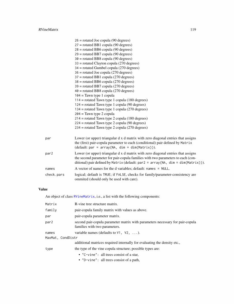
RVineMatrix 119
26 = rotated Joe copula (90 degrees)27 = rotated BB1 copula (90 degrees)28 = rotated BB6 copula (90 degrees)29 = rotated BB7 copula (90 degrees)30 = rotated BB8 copula (90 degrees)33 = rotated Clayton copula (270 degrees)34 = rotated Gumbel copula (270 degrees)36 = rotated Joe copula (270 degrees)37 = rotated BB1 copula (270 degrees)38 = rotated BB6 copula (270 degrees)39 = rotated BB7 copula (270 degrees)40 = rotated BB8 copula (270 degrees)104 = Tawn type 1 copula114 = rotated Tawn type 1 copula (180 degrees)124 = rotated Tawn type 1 copula (90 degrees)134 = rotated Tawn type 1 copula (270 degrees)204 = Tawn type 2 copula214 = rotated Tawn type 2 copula (180 degrees)224 = rotated Tawn type 2 copula (90 degrees)234 = rotated Tawn type 2 copula (270 degrees)
par Lower (or upper) triangular d x d matrix with zero diagonal entries that assignsthe (first) pair-copula parameter to each (conditional) pair defined by Matrix(default: par = array(NA, dim = dim(Matrix))).
par2 Lower (or upper) triangular d x d matrix with zero diagonal entries that assignsthe second parameter for pair-copula families with two parameters to each (con-ditional) pair defined by Matrix (default: par2 = array(NA, dim = dim(Matrix))).
names A vector of names for the d variables; default: names = NULL.
check.pars logical; default is TRUE; if FALSE, checks for family/parameter-consistency areommited (should only be used with care).
Value
An object of class RVineMatrix, i.e., a list with the following components:
Matrix R-vine tree structure matrix.
family pair-copula family matrix with values as above.
par pair-copula parameter matrix.
par2 second pair-copula parameter matrix with parameters necessary for pair-copulafamilies with two parameters.
names variable names (defaults to V1, V2, ...).MaxMat, CondDistr
additional matrices required internally for evaluating the density etc.,
type the type of the vine copula structure; possible types are:
• "C-vine": all trees consist of a star,• "D-vine": all trees consist of a path,
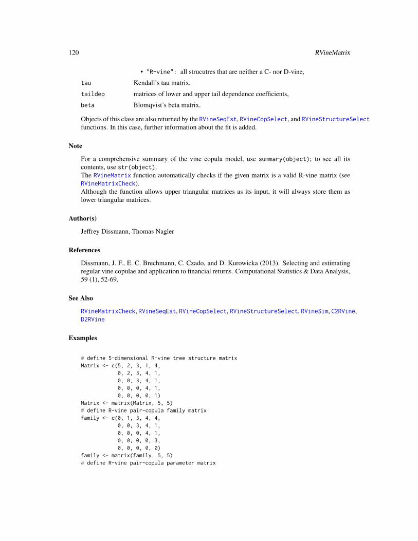
120 RVineMatrix
• "R-vine": all strucutres that are neither a C- nor D-vine,
tau Kendall’s tau matrix,
taildep matrices of lower and upper tail dependence coefficients,
beta Blomqvist’s beta matrix.
Objects of this class are also returned by the RVineSeqEst, RVineCopSelect, and RVineStructureSelectfunctions. In this case, further information about the fit is added.
Note
For a comprehensive summary of the vine copula model, use summary(object); to see all itscontents, use str(object).The RVineMatrix function automatically checks if the given matrix is a valid R-vine matrix (seeRVineMatrixCheck).Although the function allows upper triangular matrices as its input, it will always store them aslower triangular matrices.
Author(s)
Jeffrey Dissmann, Thomas Nagler
References
Dissmann, J. F., E. C. Brechmann, C. Czado, and D. Kurowicka (2013). Selecting and estimatingregular vine copulae and application to financial returns. Computational Statistics & Data Analysis,59 (1), 52-69.
See Also
RVineMatrixCheck, RVineSeqEst, RVineCopSelect, RVineStructureSelect, RVineSim, C2RVine,D2RVine
Examples
# define 5-dimensional R-vine tree structure matrixMatrix <- c(5, 2, 3, 1, 4,
0, 2, 3, 4, 1,0, 0, 3, 4, 1,0, 0, 0, 4, 1,0, 0, 0, 0, 1)
Matrix <- matrix(Matrix, 5, 5)# define R-vine pair-copula family matrixfamily <- c(0, 1, 3, 4, 4,
0, 0, 3, 4, 1,0, 0, 0, 4, 1,0, 0, 0, 0, 3,0, 0, 0, 0, 0)
family <- matrix(family, 5, 5)# define R-vine pair-copula parameter matrix
RVineMatrixCheck 121
par <- c(0, 0.2, 0.9, 1.5, 3.9,0, 0, 1.1, 1.6, 0.9,0, 0, 0, 1.9, 0.5,0, 0, 0, 0, 4.8,0, 0, 0, 0, 0)
par <- matrix(par, 5, 5)# define second R-vine pair-copula parameter matrixpar2 <- matrix(0, 5, 5)
## define RVineMatrix objectRVM <- RVineMatrix(Matrix = Matrix, family = family,
par = par, par2 = par2,names = c("V1", "V2", "V3", "V4", "V5"))
## see the object's content or a summarystr(RVM)summary(RVM)
## inspect the model using plots## Not run: plot(RVM) # tree structurecontour(RVM) # contour plots of all pair-copulas
## simulate from the vine copula modelplot(RVineSim(500, RVM))
RVineMatrixCheck R-Vine Matrix Check
Description
The given matrix is tested to be a valid R-vine matrix.
Usage
RVineMatrixCheck(M)
Arguments
M A dxd vine matrix.
Value
code 1 for OK;-4 matrix is neither lower nor upper triangular;-3 diagonal can not be put in order d:1;-2 for not permutation of j:d in column d-j;-1 if cannot find proper binary array from array in natural order.
122 RVineMatrixCheck
Note
The matrix M do not have to be given in natural order or the diagonal in order d:1. The test checksif it can be done in order to be a valid R-vine matrix.If a function in this package needs the natural order the RVineMatrix object is automatically "nor-malized".The function RVineMatrix automatically checks if the given R-vine matrix is valid.
Author(s)
Harry Joe
References
Joe H, Cooke RM and Kurowicka D (2011). Regular vines: generation algorithm and numberof equivalence classes. In Dependence Modeling: Vine Copula Handbook, pp 219–231. WorldScientific, Singapore.
See Also
RVineMatrix
Examples
A1 <- matrix(c(6, 0, 0, 0, 0, 0,5, 5, 0, 0, 0, 0,3, 4, 4, 0, 0, 0,4, 3, 3, 3, 0, 0,1, 1, 2, 2, 2, 0,2, 2, 1, 1, 1, 1), 6, 6, byrow = TRUE)
b1 <- RVineMatrixCheck(A1)print(b1)# improper vine matrix, code=-1A2 <- matrix(c(6, 0, 0, 0, 0, 0,
5, 5, 0, 0, 0, 0,4, 4, 4, 0, 0, 0,1, 3, 3, 3, 0, 0,3, 1, 2, 2, 2, 0,2, 2, 1, 1, 1,1 ), 6, 6, byrow = TRUE)
b2 <- RVineMatrixCheck(A2)print(b2)# improper vine matrix, code=-2A3 <- matrix(c(6, 0, 0, 0, 0, 0,
3, 5, 0, 0, 0, 0,3, 4, 4, 0, 0, 0,4, 3, 3, 3, 0, 0,1, 1, 2, 2, 2, 0,2, 2, 1, 1, 1, 1), 6, 6, byrow = TRUE)
b3 <- RVineMatrixCheck(A3)print(b3)
RVineMatrixNormalize 123
RVineMatrixNormalize Normalization of R-Vine Matrix
Description
An RVineMatrix is permuted to achieve a natural ordering (i.e. diag(RVM$Matrix) == d:1)
Usage
RVineMatrixNormalize(RVM)
Arguments
RVM RVineMatrix defining the R-vine structure
Value
RVM An RVineMatrix in natural ordering with entries in RVM$names keeping track ofthe reordering.
Examples
Matrix <- matrix(c(5, 2, 3, 1, 4,0, 2, 3, 4, 1,0, 0, 3, 4, 1,0, 0, 0, 4, 1,0, 0, 0, 0, 1), 5, 5)
family <- matrix(1,5,5)
par <- matrix(c(0, 0.2, 0.9, 0.5, 0.8,0, 0, 0.1, 0.6, 0.9,0, 0, 0, 0.7, 0.5,0, 0, 0, 0, 0.8,0, 0, 0, 0, 0), 5, 5)
# define RVineMatrix objectRVM <- RVineMatrix(Matrix, family, par)
# normalise the RVineRVineMatrixNormalize(RVM)
124 RVineMatrixSample
RVineMatrixSample Randomv sampling of R-Vine matices
Description
Sample R-Vine matrices based on the algorithm of Joe et al. (2011).
Usage
RVineMatrixSample(d, size = 1, naturalOrder = FALSE)
Arguments
d Dimension of the R-Vine matrices.
size Number of matrices to sample.
naturalOrder Should the matrices be in the natural order (default: naturalOrder = FALSE).
Value
A list of length size with each element containing one R-Vine matrix.
Note
For some reason, our implementaion of Joe et al.’s algorithm always returns a star in the first tree.To fix this, we sample a vine matrix of dimension d + 1 and remove the first tree afterwards
Author(s)
Thibault Vatter
References
Joe H, Cooke RM and Kurowicka D (2011). Regular vines: generation algorithm and numberof equivalence classes. In Dependence Modeling: Vine Copula Handbook, pp 219–231. WorldScientific, Singapore.
See Also
RVineMatrix, RVineMatrixCheck
Examples
# Matrix and sample sizesd <- 10size <- 5
# Sample R-vine matricesRVM <- RVineMatrixSample(d, size)
RVineMLE 125
sapply(RVM, RVineMatrixCheck)
# Sample R-vine matrices in the natural orderRVM <- RVineMatrixSample(d, size, naturalOrder = TRUE)sapply(RVM, RVineMatrixCheck)
RVineMLE Maximum Likelihood Estimation of an R-Vine Copula Model
Description
This function calculates the maxiumum likelihood estimate (MLE) of the R-vine copula modelparameters using sequential estimates as initial values (if not provided).
Usage
RVineMLE(data, RVM, start = RVM$par, start2 = RVM$par2, maxit = 200,max.df = 30, max.BB = list(BB1 = c(5, 6), BB6 = c(6, 6), BB7 = c(5, 6),BB8 = c(6, 1)), grad = FALSE, hessian = FALSE, se = FALSE, ...)
Arguments
data An N x d data matrix (with uniform margins).
RVM An RVineMatrix object including the structure and the pair-copula families andparameters (if known).
start Lower triangular d x d matrix with zero diagonal entries with starting values forthe pair-copula parameters (optional; otherwise they are calculated viaRVineSeqEst; default: start = RVM$par).
start2 Lower triangular d x d matrix with zero diagonal entries with starting values forthe second parameters of pair-copula families with two parameters (optional;otherwise they are calculated via RVineSeqEst; default: start2 = RVM$par2).
maxit The maximum number of iteration steps (optional; default: maxit = 200).
max.df Numeric; upper bound for the estimation of the degrees of freedom parameterof the t-copula (default: max.df = 30; for more details see BiCopEst).
max.BB List; upper bounds for the estimation of the two parameters (in absolute values)of the BB1, BB6, BB7 and BB8 copulas(default: max.BB = list(BB1=c(5,6),BB6=c(6,6),BB7=c(5,6),BB8=c(6,1))).
grad If RVM$family only contains one parameter copula families or the t-copulathe analytical gradient can be used for maximization of the log-likelihood (seeRVineGrad; default: grad = FALSE).
hessian Logical; whether the Hessian matrix of parameter estimates is estimated (de-fault: hessian = FALSE). Note that this is not the Hessian Matrix calculatedvia RVineHessian but via finite differences.
126 RVineMLE
se Logical; whether standard errors of parameter estimates are estimated on thebasis of the Hessian matrix (see above; default: se = FALSE).
... Further arguments for optim (e.g. factr controls the convergence of the "L-BFGS-B" method, or trace, a non-negative integer, determines if tracing infor-mation on the progress of the optimization is produced.)For more details see the documentation of optim.
Value
RVM RVineMatrix object with the calculated parameters stored in RVM$par and RVM$par2.Additional information about the fit is added (e.g., log-likelihood, AIC, BIC).
value Optimized log-likelihood value corresponding to the estimated pair-copula pa-rameters.
convergence An integer code indicating either successful convergence (convergence = 0)or an error:1 = the iteration limit maxit has been reached51 = a warning from the "L-BFGS-B" method; see component message forfurther details52 = an error from the "L-BFGS-B" method; see component message for furtherdetails
message A character string giving any additional information returned by optim, or NULL.
counts A two-element integer vector giving the number of calls to fn and gr respec-tively. This excludes those calls needed to compute the Hessian, if requested,and any calls to fn to compute a finite-difference approximation to the gradient.
hessian If hessian = TRUE, the Hessian matrix is returned. Its calculation is on thebasis of finite differences (output of optim).
Note
RVineMLE uses the L-BFGS-B method for optimization.If the analytical gradient is used for maximization, computations may be up to 10 times faster thanusing finite differences.
Author(s)
Ulf Schepsmeier, Jeffrey Dissmann
References
Dissmann, J. F., E. C. Brechmann, C. Czado, and D. Kurowicka (2013). Selecting and estimatingregular vine copulae and application to financial returns. Computational Statistics & Data Analysis,59 (1), 52-69.
Stoeber, J. and U. Schepsmeier (2013). Estimating standard errors in regular vine copula models.Computational Statistics, 1-29 http://link.springer.com/article/10.1007/s00180-013-0423-8#.
See Also
RVineSeqEst, RVineStructureSelect, RVineMatrix, RVineGrad, RVineHessian
RVinePar2Beta 127
Examples
# define 5-dimensional R-vine tree structure matrixMatrix <- c(5, 2, 3, 1, 4,
0, 2, 3, 4, 1,0, 0, 3, 4, 1,0, 0, 0, 4, 1,0, 0, 0, 0, 1)
Matrix <- matrix(Matrix, 5, 5)
# define R-vine pair-copula family matrixfamily <- c(0, 1, 3, 4, 4,
0, 0, 3, 4, 1,0, 0, 0, 4, 1,0, 0, 0, 0, 3,0, 0, 0, 0, 0)
family <- matrix(family, 5, 5)
# define R-vine pair-copula parameter matrixpar <- c(0, 0.2, 0.9, 1.5, 3.9,
0, 0, 1.1, 1.6, 0.9,0, 0, 0, 1.9, 0.5,0, 0, 0, 0, 4.8,0, 0, 0, 0, 0)
par <- matrix(par, 5, 5)
# define second R-vine pair-copula parameter matrixpar2 <- matrix(0, 5, 5)
# define RVineMatrix objectRVM <- RVineMatrix(Matrix = Matrix, family = family,
par = par, par2 = par2,names = c("V1", "V2", "V3", "V4", "V5"))
# simulate a sample of size 300 from the R-vine copula modelset.seed(123)simdata <- RVineSim(300, RVM)
# compute the MLEmle <- RVineMLE(simdata, RVM, grad = TRUE, trace = 0)
# compare parametersround(mle$RVM$par - RVM$par, 2)
RVinePar2Beta Blomqvist’s Beta Values of an R-Vine Copula Model
128 RVinePar2Beta
Description
This function computes the values of Blomqvist’s beta corresponding to the parameters of an R-vinecopula model.
Usage
RVinePar2Beta(RVM, check.pars = TRUE)
Arguments
RVM An RVineMatrix object.Note that the Student’s t-copula is not allowed since the CDF of the t-copula isnot implemented (see BiCopCDF and BiCopPar2Beta).
check.pars logical; default is TRUE; if FALSE, checks for family/parameter-consistency areommited (should only be used with care).
Value
Matrix with the same structure as the family and parameter matrices of the RVineMatrix object RVMwhere the entries are values of Blomqvist’s beta corresponding to the families and parameters ofthe R-vine copula model given by RVM.
Author(s)
Ulf Schepsmeier
See Also
RVineMatrix, BiCopPar2Beta
Examples
# define 5-dimensional R-vine tree structure matrixMatrix <- c(5, 2, 3, 1, 4,
0, 2, 3, 4, 1,0, 0, 3, 4, 1,0, 0, 0, 4, 1,0, 0, 0, 0, 1)
Matrix <- matrix(Matrix, 5, 5)
# define R-vine pair-copula family matrixfamily <- c(0, 1, 3, 4, 4,
0, 0, 3, 4, 1,0, 0, 0, 4, 1,0, 0, 0, 0, 3,0, 0, 0, 0, 0)
family <- matrix(family, 5, 5)
# define R-vine pair-copula parameter matrixpar <- c(0, 0.2, 0.9, 1.5, 3.9,
RVinePar2Tau 129
0, 0, 1.1, 1.6, 0.9,0, 0, 0, 1.9, 0.5,0, 0, 0, 0, 4.8,0, 0, 0, 0, 0)
par <- matrix(par, 5, 5)
# define second R-vine pair-copula parameter matrixpar2 <- matrix(0, 5, 5)
# define RVineMatrix objectRVM <- RVineMatrix(Matrix = Matrix, family = family,
par = par, par2 = par2,names = c("V1", "V2", "V3", "V4", "V5"))
# compute the Blomqvist's beta valuesBlomBeta <- RVinePar2Beta(RVM)
RVinePar2Tau Kendall’s Tau Values of an R-Vine Copula Model
Description
This function computes the values of Kendall’s tau corresponding to the parameters of an R-vinecopula model.
Usage
RVinePar2Tau(RVM, check.pars = TRUE)
Arguments
RVM An RVineMatrix object.
check.pars logical; default is TRUE; if FALSE, checks for family/parameter-consistency areommited (should only be used with care).
Value
Matrix with the same structure as the family and parameter matrices of the RVineMatrix object RVMwhere the entries are values of Kendall’s tau corresponding to the families and parameters of theR-vine copula model given by RVM.
Author(s)
Jeffrey Dissmann
See Also
RVineMatrix, BiCopPar2Tau
130 RVinePDF
Examples
# define 5-dimensional R-vine tree structure matrixMatrix <- c(5, 2, 3, 1, 4,
0, 2, 3, 4, 1,0, 0, 3, 4, 1,0, 0, 0, 4, 1,0, 0, 0, 0, 1)
Matrix <- matrix(Matrix, 5, 5)
# define R-vine pair-copula family matrixfamily <- c(0, 1, 3, 4, 4,
0, 0, 3, 4, 1,0, 0, 0, 4, 1,0, 0, 0, 0, 3,0, 0, 0, 0, 0)
family <- matrix(family, 5, 5)
# define R-vine pair-copula parameter matrixpar <- c(0, 0.2, 0.9, 1.5, 3.9,
0, 0, 1.1, 1.6, 0.9,0, 0, 0, 1.9, 0.5,0, 0, 0, 0, 4.8,0, 0, 0, 0, 0)
par <- matrix(par, 5, 5)
# define second R-vine pair-copula parameter matrixpar2 <- matrix(0, 5, 5)
# define RVineMatrix objectRVM <- RVineMatrix(Matrix = Matrix, family = family,
par = par, par2 = par2,names = c("V1", "V2", "V3", "V4", "V5"))
# compute the Kendall's tau valuestau <- RVinePar2Tau(RVM)
RVinePDF PDF of an R-Vine Copula Model
Description
This function calculates the probability density function of a d-dimensional R-vine copula.
Usage
RVinePDF(newdata, RVM, verbose = TRUE)
RVinePDF 131
Arguments
newdata An N x d data matrix that specifies where the density shall be evaluated.
RVM An RVineMatrix object including the structure and the pair-copula families andparameters.
verbose In case something goes wrong, additional output will be plotted.
Details
The density of a d-dimensional R-vine copula with d−1 trees and corresponding edge setsE1, ..., Ed−1is given by
d−1∏`=1
∏e∈E`
cj(e),k(e)|D(e)(F (uj(e)|uD(e)), F (uk(e)|uD(e))|θj(e),k(e)|D(e)),
where u = (u1, ..., ud)′ ∈ [0, 1]d. Further cj(e),k(e)|D(e) denotes a bivariate copula density associ-
ated to an edge e and with parameter(s) θj(e),k(e)|D(e). Conditional distribution functions such asF (uj(e)|uD(e)) are obtained recursively using the relationship
h(u|v,θ) := F (u|v) = dCuvj |v−j(F (u|v−j), F (vj |v−j))/dF (vj |v−j),
where Cuvj |v−jis a bivariate copula distribution function with parameter(s) θ and v−j denotes a
vector with the j-th component vj removed. The notation of h-functions is introduced for conve-nience. For more details see Dissmann et al. (2013).
The function is actually just a wrapper to RVineLogLik.
Author(s)
Thomas Nagler
References
Dissmann, J. F., E. C. Brechmann, C. Czado, and D. Kurowicka (2013). Selecting and estimatingregular vine copulae and application to financial returns. Computational Statistics & Data Analysis,59 (1), 52-69.
See Also
BiCopHfunc, RVineMatrix, RVineMLE, RVineAIC, RVineBIC
Examples
# define 5-dimensional R-vine tree structure matrixMatrix <- c(5, 2, 3, 1, 4,
0, 2, 3, 4, 1,0, 0, 3, 4, 1,0, 0, 0, 4, 1,0, 0, 0, 0, 1)
Matrix <- matrix(Matrix, 5, 5)
132 RVinePIT
# define R-vine pair-copula family matrixfamily <- c(0, 1, 3, 4, 4,
0, 0, 3, 4, 1,0, 0, 0, 4, 1,0, 0, 0, 0, 3,0, 0, 0, 0, 0)
family <- matrix(family, 5, 5)
# define R-vine pair-copula parameter matrixpar <- c(0, 0.2, 0.9, 1.5, 3.9,
0, 0, 1.1, 1.6, 0.9,0, 0, 0, 1.9, 0.5,0, 0, 0, 0, 4.8,0, 0, 0, 0, 0)
par <- matrix(par, 5, 5)
# define second R-vine pair-copula parameter matrixpar2 <- matrix(0, 5, 5)
# define RVineMatrix objectRVM <- RVineMatrix(Matrix = Matrix, family = family,
par = par, par2 = par2,names = c("V1", "V2", "V3", "V4", "V5"))
# compute the density at (0.1, 0.2, 0.3, 0.4, 0.5)RVinePDF(c(0.1, 0.2, 0.3, 0.4, 0.5), RVM)
RVinePIT Probability Integral Transformation for R-Vine Copula Models
Description
This function applies the probability integral transformation (PIT) for R-vine copula models togiven copula data.
Usage
RVinePIT(data, RVM)
Arguments
data An N x d data matrix (with uniform margins).
RVM RVineMatrix objects of the R-vine model.
RVinePIT 133
Details
The multivariate probability integral transformation (PIT) of Rosenblatt (1952) transforms the cop-ula data u = (u1, . . . , ud) with a given multivariate copula C into independent data in [0, 1]d, whered is the dimension of the data set.
Let u = (u1, . . . , ud) denote copula data of dimension d. Further let C be the joint cdf of u =(u1, . . . , ud). Then Rosenblatt’s transformation of u, denoted as y = (y1, . . . , yd), is defined as
y1 := u1, y2 := C(u2|u1), . . . yd := C(ud|u1, . . . , ud−1),
where C(uk|u1, . . . , uk−1) is the conditional copula of Uk given U1 = u1, . . . , Uk−1 = uk−1, k =2, . . . , d. The data vector y = (y1, . . . , yd) is now i.i.d. with yi ∼ U [0, 1]. The algorithm for theR-vine PIT is given in the appendix of Schepsmeier (2015).
Value
An N x d matrix of PIT data from the given R-vine copula model.
Author(s)
Ulf Schepsmeier
References
Rosenblatt, M. (1952). Remarks on a Multivariate Transformation. The Annals of MathematicalStatistics 23 (3), 470-472.
Schepsmeier, U. (2015) Efficient information based goodness-of-fit tests for vine copula modelswith fixed margins. Journal of Multivariate Analysis 138, 34-52.
See Also
RVineGofTest
Examples
# load data setdata(daxreturns)
# select the R-vine structure, families and parametersRVM <- RVineStructureSelect(daxreturns[,1:3], c(1:6))
# PIT datapit <- RVinePIT(daxreturns[,1:3], RVM)
par(mfrow = c(1,2))plot(daxreturns[,1], daxreturns[,2]) # correlated dataplot(pit[,1], pit[,2]) # i.i.d. data
cor(pit, method = "kendall")
134 RVineSeqEst
RVineSeqEst Sequential Estimation of an R-Vine Copula Model
Description
This function sequentially estimates the pair-copula parameters of a d-dimensional R-vine copulamodel as specified by the corresponding RVineMatrix object.
Usage
RVineSeqEst(data, RVM, method = "mle", se = FALSE, max.df = 30,max.BB = list(BB1 = c(5, 6), BB6 = c(6, 6), BB7 = c(5, 6), BB8 = c(6, 1)),progress = FALSE, weights = NA, cores = 1)
Arguments
data An N x d data matrix (with uniform margins).
RVM An RVineMatrix object including the structure, the pair-copula families and thepair-copula parameters (if they are known).
method indicates the estimation method: either maximum likelihood estimation (method = "mle";default) or inversion of Kendall’s tau (method = "itau"). For method = "itau"only one parameter families and the Student t copula can be used (family =1,2,3,4,5,6,13,14,16,23,24,26,33,34 or 36). For the t-copula, par2 isfound by a crude profile likelihood optimization over the interval (2, 10].
se Logical; whether standard errors are estimated (default: se = FALSE).
max.df Numeric; upper bound for the estimation of the degrees of freedom parameterof the t-copula (default: max.df = 30; for more details see BiCopEst).
max.BB List; upper bounds for the estimation of the two parameters (in absolute values)of the BB1, BB6, BB7 and BB8 copulas(default: max.BB = list(BB1=c(5,6),BB6=c(6,6),BB7=c(5,6),BB8=c(6,1))).
progress Logical; whether the pairwise estimation progress is printed (default: progress = FALSE).
weights Numerical; weights for each observation (opitional).
cores integer; if cores > 1, estimation will be parallized within each tree (usingforeach). However, the overhead caused by parallelization is likely to make thefunction run slower unless sample size is really large and method = "itau".
Details
The pair-copula parameter estimation is performed tree-wise, i.e., for each R-vine tree the resultsfrom the previous tree(s) are used to calculate the new copula parameters using BiCopEst.
RVineSeqEst 135
Value
An RVineMatrix object with the sequentially estimated parameters stored in RVM$par and RVM$par2.The object is augmented by the following information about the fit:
se, se2 standard errors for the parameter estimates (if se = TRUE); note that these areonly approximate since they do not account for the sequential nature of the esti-mation,
nobs number of observations,logLik, pair.logLik
log likelihood (overall and pairwise)
AIC, pair.AIC Aikaike’s Informaton Criterion (overall and pairwise),
BIC, pair.BIC Bayesian’s Informaton Criterion (overall and pairwise),
emptau matrix of empirical values of Kendall’s tau,p.value.indeptest
matrix of p-values of the independence test.
Note
For a comprehensive summary of the fitted model, use summary(object); to see all its contents,use str(object).
Author(s)
Ulf Schepsmeier, Jeffrey Dissmann, Thomas Nagler
See Also
RVineMatrix, BiCop, BiCopEst, plot.RVineMatrix, contour.RVineMatrix, foreach
Examples
# define 5-dimensional R-vine tree structure matrixMatrix <- c(5, 2, 3, 1, 4,
0, 2, 3, 4, 1,0, 0, 3, 4, 1,0, 0, 0, 4, 1,0, 0, 0, 0, 1)
Matrix <- matrix(Matrix, 5, 5)
# define R-vine pair-copula family matrixfamily <- c(0, 1, 3, 4, 4,
0, 0, 3, 4, 1,0, 0, 0, 4, 1,0, 0, 0, 0, 3,0, 0, 0, 0, 0)
family <- matrix(family, 5, 5)
# define R-vine pair-copula parameter matrix
136 RVineSim
par <- c(0, 0.2, 0.9, 1.5, 3.9,0, 0, 1.1, 1.6, 0.9,0, 0, 0, 1.9, 0.5,0, 0, 0, 0, 4.8,0, 0, 0, 0, 0)
par <- matrix(par, 5, 5)
# define second R-vine pair-copula parameter matrixpar2 <- matrix(0, 5, 5)
# define RVineMatrix objectRVM <- RVineMatrix(Matrix = Matrix, family = family,
par = par, par2 = par2,names = c("V1", "V2", "V3", "V4", "V5"))
# simulate a sample of size 300 from the R-vine copula modelset.seed(123)simdata <- RVineSim(300, RVM)
# sequential estimationsummary(RVineSeqEst(simdata, RVM, method = "itau", se = TRUE))summary(RVineSeqEst(simdata, RVM, method = "mle", se = TRUE))
RVineSim Simulation from an R-Vine Copula Model
Description
This function simulates from a given R-vine copula model.
Usage
RVineSim(N, RVM, U = NULL)
Arguments
N Number of d-dimensional observations to simulate.
RVM An RVineMatrix object containing the information of the R-vine copula model.
U If not NULL, an (N,d)-matrix of U[0,1] random variates to be transformed to thecopula sample.
Value
An N x d matrix of data simulated from the given R-vine copula model.
Author(s)
Jeffrey Dissmann
RVineSim 137
References
Dissmann, J. F., E. C. Brechmann, C. Czado, and D. Kurowicka (2013). Selecting and estimatingregular vine copulae and application to financial returns. Computational Statistics & Data Analysis,59 (1), 52-69.
See Also
RVineMatrix, BiCopSim
Examples
# define 5-dimensional R-vine tree structure matrixMatrix <- c(5, 2, 3, 1, 4,
0, 2, 3, 4, 1,0, 0, 3, 4, 1,0, 0, 0, 4, 1,0, 0, 0, 0, 1)
Matrix <- matrix(Matrix, 5, 5)
# define R-vine pair-copula family matrixfamily <- c(0, 1, 3, 4, 4,
0, 0, 3, 4, 1,0, 0, 0, 4, 1,0, 0, 0, 0, 3,0, 0, 0, 0, 0)
family <- matrix(family, 5, 5)
# define R-vine pair-copula parameter matrixpar <- c(0, 0.2, 0.9, 1.5, 3.9,
0, 0, 1.1, 1.6, 0.9,0, 0, 0, 1.9, 0.5,0, 0, 0, 0, 4.8,0, 0, 0, 0, 0)
par <- matrix(par, 5, 5)
# define second R-vine pair-copula parameter matrixpar2 <- matrix(0, 5, 5)
# define RVineMatrix objectRVM <- RVineMatrix(Matrix = Matrix, family = family,
par = par, par2 = par2,names = c("V1", "V2", "V3", "V4", "V5"))
# simulate a sample of size 300 from the R-vine copula modelset.seed(123)simdata <- RVineSim(300, RVM)
138 RVineStdError
RVineStdError Standard Errors of an R-Vine Copula Model
Description
This function calculates the standard errors of a d-dimensional R-vine copula model given the Hes-sian matrix.
Usage
RVineStdError(hessian, RVM)
Arguments
hessian The Hessian matrix of the given R-vine.RVM An RVineMatrix object including the structure, the pair-copula families, and
the parameters.
Value
se The calculated standard errors for the first parameter matrix. The entries areordered with respect to the ordering of the RVM$par matrix.
se2 The calculated standard errors for the second parameter matrix.
Note
The negative Hessian matrix should be positive semidefinite. Otherwise NAs will be returned insome entries and the non-NA entries may be wrong. If the negaive Hessian matrix is negativedefinite, then one could try a near positive matrix. The package Matrix provides a function callednearPD to estimate a matrix which is positive definite and close to the given matrix.
Author(s)
Ulf Schepsmeier, Jakob Stoeber
References
Dissmann, J. F., E. C. Brechmann, C. Czado, and D. Kurowicka (2013). Selecting and estimatingregular vine copulae and application to financial returns. Computational Statistics & Data Analysis,59 (1), 52-69.
Schepsmeier, U. and J. Stoeber (2014) Derivatives and Fisher information of bivariate copulas.Statistical Papers, 55(2), 525-542. online first: http://link.springer.com/article/10.1007/s00362-013-0498-x.
Web supplement: Derivatives and Fisher Information of bivariate copulas. http://mediatum.ub.tum.de/node?id=1119201
Stoeber, J. and U. Schepsmeier (2013). Estimating standard errors in regular vine copula models.Computational Statistics, 28 (6), 2679-2707 http://link.springer.com/article/10.1007/s00180-013-0423-8#.
RVineStdError 139
See Also
BiCopDeriv, BiCopDeriv2, BiCopHfuncDeriv, BiCopHfuncDeriv2,RVineMatrix, RVineHessian, RVineGrad
Examples
# define 5-dimensional R-vine tree structure matrixMatrix <- c(5, 2, 3, 1, 4,
0, 2, 3, 4, 1,0, 0, 3, 4, 1,0, 0, 0, 4, 1,0, 0, 0, 0, 1)
Matrix <- matrix(Matrix, 5, 5)
# define R-vine pair-copula family matrixfamily <- c(0, 1, 3, 4, 4,
0, 0, 3, 4, 1,0, 0, 0, 4, 1,0, 0, 0, 0, 3,0, 0, 0, 0, 0)
family <- matrix(family, 5, 5)
# define R-vine pair-copula parameter matrixpar <- c(0, 0.2, 0.9, 1.5, 3.9,
0, 0, 1.1, 1.6, 0.9,0, 0, 0, 1.9, 0.5,0, 0, 0, 0, 4.8,0, 0, 0, 0, 0)
par <- matrix(par, 5, 5)
# define second R-vine pair-copula parameter matrixpar2 <- matrix(0, 5, 5)
# define RVineMatrix objectRVM <- RVineMatrix(Matrix = Matrix, family = family,
par = par, par2 = par2,names = c("V1", "V2", "V3", "V4", "V5"))
# simulate a sample of size 300 from the R-vine copula modelset.seed(123)simdata <- RVineSim(300, RVM)
# compute the Hessian matrix of the first row of the dataout2 <- RVineHessian(simdata,RVM)
# get the standard errorsRVineStdError(out2$hessian, RVM)
140 RVineStructureSelect
RVineStructureSelect Sequential Specification of R- and C-Vine Copula Models
Description
This function fits either an R- or a C-vine copula model to a d-dimensional copula data set. Treestructures are determined and appropriate pair-copula families are selected using BiCopSelect andestimated sequentially (forward selection of trees).
Usage
RVineStructureSelect(data, familyset = NA, type = 0,selectioncrit = "AIC", indeptest = FALSE, level = 0.05,trunclevel = NA, progress = FALSE, weights = NA, treecrit = "tau",se = FALSE, rotations = TRUE, method = "mle", cores = 1)
Arguments
data An N x d data matrix (with uniform margins).
familyset An integer vector of pair-copula families to select from. The vector has to in-clude at least one pair-copula family that allows for positive and one that allowsfor negative dependence. Not listed copula families might be included to betterhandle limit cases. If familyset = NA (default), selection among all possiblefamilies is performed. Coding of pair-copula families is the same as in BiCop.
type Type of the vine model to be specified:0 or "RVine" = R-vine (default)1 or "CVine" = C-vineC- and D-vine copula models with pre-specified order can be specified usingCDVineCopSelect of the package CDVine. Similarly, R-vine copula modelswith pre-specified tree structure can be specified using RVineCopSelect.
selectioncrit Character indicating the criterion for pair-copula selection. Possible choices:selectioncrit = "AIC"(default), "BIC", or "logLik" (see BiCopSelect).
indeptest logical; whether a hypothesis test for the independence of u1 and u2 is per-formed before bivariate copula selection (default: indeptest = FALSE; seeBiCopIndTest). The independence copula is chosen for a (conditional) pair ifthe null hypothesis of independence cannot be rejected.
level numeri; significance level of the independence test (default: level = 0.05).
trunclevel integer; level of truncation.
progress logical; whether the tree-wise specification progress is printed (default: progress = FALSE).
weights numeric; weights for each observation (opitional).
treecrit edge weight for Dissman’s structure selection algorithm, see Details.
se Logical; whether standard errors are estimated (default: se = FALSE).
rotations If TRUE, all rotations of the families in familyset are included.
RVineStructureSelect 141
method indicates the estimation method: either maximum likelihood estimation (method = "mle";default) or inversion of Kendall’s tau (method = "itau"). For method = "itau"only one parameter families and the Student t copula can be used (family =1,2,3,4,5,6,13,14,16,23,24,26,33,34 or 36). For the t-copula, par2 isfound by a crude profile likelihood optimization over the interval (2, 10].
cores integer; if cores > 1, estimation will be parallized within each tree (usingforeach). Note that parallelization causes substantial overhead and may beslower than single-threaded computation when dimension, sample size, or fam-ilyset are small or method = "itau".
Details
R-vine trees are selected using maximum spanning trees w.r.t. some edge weights. The mostcommonly used edge weigth is the absolute value of the empirical Kendall’s tau, say τij . Then,the following o ptimization problem is solved for each tree:
max∑
edges eij∈ in spanning tree
|τij |,
where a spanning tree is a tree on all nodes. The setting of the first tree selection step is always acomplete graph. For subsequent trees, the setting depends on the R-vine construction principles, inparticular on the proximity condition.
Some commonly used edge weights are implemented:
"tau" absolute value of empirical Kendall’s tau."rho" absolute value of empirical Spearman’s rho."AIC" Akaike information (multiplied by -1)."BIC" Bayesian information criterion (multiplied by -1)."cAIC" corrected Akaike information criterion (multiplied by -1).
If the data contain NAs, the edge weights in "tau" and "rho" are multiplied by the square root ofthe proportion of complete observations. This penalizes pairs where less observations are used.
The criteria "AIC", "BIC", and "cAIC" require estimation and model selection for all possiblepairs. This is computationally expensive and much slower than "tau" or "rho". The user canalso specify a custom function to calculate the edge weights. The function has to be of typefunction(u1, u2, weights) ... and must return a numeric value. The weigths argumentmust exist, but does not has to be used. For example, "tau" (withouth using weights) can be imple-mented as follows:function(u1, u2, weights)abs(cor(u1, u2, method = "kendall", use = "complete.obs"))
The root nodes of C-vine trees are determined similarly by identifying the node with strongestdependencies to all other nodes. That is we take the node with maximum column sum in theempirical Kendall’s tau matrix.
Note that a possible way to determine the order of the nodes in the D-vine is to identify a shortestHamiltonian path in terms of weights 1 − | ˆτij |. This can be established for example using the
142 RVineStructureSelect
package TSP. Example code is shown below.
Value
An RVineMatrix object with the selected structure (RVM$Matrix) and families (RVM$family) aswell as sequentially estimated parameters stored in RVM$par and RVM$par2. The object is aug-mented by the following information about the fit:
se, se2 standard errors for the parameter estimates; note that these are only approximatesince they do not account for the sequential nature of the estimation,
nobs number of observations,logLik, pair.logLik
log likelihood (overall and pairwise)
AIC, pair.AIC Aikaike’s Informaton Criterion (overall and pairwise),
BIC, pair.BIC Bayesian’s Informaton Criterion (overall and pairwise),
emptau matrix of empirical values of Kendall’s tau,p.value.indeptest
matrix of p-values of the independence test.
Note
For a comprehensive summary of the vine copula model, use summary(object); to see all itscontents, use str(object).
Author(s)
Jeffrey Dissmann, Eike Brechmann, Ulf Schepsmeier, Thomas Nagler
References
Brechmann, E. C., C. Czado, and K. Aas (2012). Truncated regular vines in high dimensions withapplications to financial data. Canadian Journal of Statistics 40 (1), 68-85.
Dissmann, J. F., E. C. Brechmann, C. Czado, and D. Kurowicka (2013). Selecting and estimatingregular vine copulae and application to financial returns. Computational Statistics & Data Analysis,59 (1), 52-69.
See Also
RVineMatrix, BiCop, RVineCopSelect, plot.RVineMatrix, contour.RVineMatrix, foreach
Examples
# load data setdata(daxreturns)
# select the R-vine structure, families and parameters# using only the first 4 variables and the first 250 observations# we allow for the copula families: Gauss, t, Clayton, Gumbel, Frank and Joe
RVineTreePlot 143
daxreturns <- daxreturns[1:250, 1:4]RVM <- RVineStructureSelect(daxreturns, c(1:6), progress = TRUE)
## see the object's content or a summarystr(RVM)summary(RVM)
## inspect the fitted model using plots## Not run: plot(RVM) # tree structurecontour(RVM) # contour plots of all pair-copulas
## estimate a C-vine copula model with only Clayton, Gumbel and Frank copulasCVM <- RVineStructureSelect(daxreturns, c(3,4,5), "CVine")
## determine the order of the nodes in a D-vine using the package TSPlibrary(TSP)d <- dim(daxreturns)[2]M <- 1 - abs(TauMatrix(daxreturns))hamilton <- insert_dummy(TSP(M), label = "cut")sol <- solve_TSP(hamilton, method = "repetitive_nn")order <- cut_tour(sol, "cut")DVM <- D2RVine(order, family = rep(0,d*(d-1)/2), par = rep(0, d*(d-1)/2))RVineCopSelect(daxreturns, c(1:6), DVM$Matrix)
RVineTreePlot Visualisation of R-Vine Tree Structure
Description
Function is deprecated since VineCopula 2.0. Use plot.RVineMatrix instead.
Usage
RVineTreePlot(x, tree = "ALL", type = 0, edge.labels = NULL,legend.pos = "bottomleft", interactive = FALSE, ...)
Arguments
x RVineMatrix object.
tree "ALL" or integer vector; specifies which trees are plotted.
type integer; specifies how to make use of variable names:0 = variable names are ignored,1 = variable names are used to annotate vertices,2 = uses numbers in plot and adds a legend for variable names.
edge.labels character; either a vector of edge labels or one of the following:"family" = pair-copula family abbreviation (see BiCopName),"par" = pair-copula parameters,
144 RVineVuongTest
"tau" = pair-copula Kendall’s tau (by conversion of parameters)"family-par" = pair-copula family and parameters"family-tau" = pair-copula family and Kendall’s tau.
legend.pos the x argument for legend.
interactive logical; if TRUE, the user is asked to adjust the positioning of vertices with hismouse.
... Arguments passed to plot.network.
Author(s)
Thomas Nagler
See Also
plot.RVineMatrix
RVineVuongTest Vuong Test Comparing Two R-Vine Copula Models
Description
This function performs a Vuong test between two d-dimensional R-vine copula models as specifiedby their RVineMatrix objects.
Usage
RVineVuongTest(data, RVM1, RVM2)
Arguments
data An N x d data matrix (with uniform margins).
RVM1, RVM2 RVineMatrix objects of models 1 and 2.
Details
The likelihood-ratio based test proposed by Vuong (1989) can be used for comparing non-nestedmodels. For this let c1 and c2 be two competing vine copulas in terms of their densities and withestimated parameter sets θ1 and θ2. We then compute the standardized sum, ν, of the log differencesof their pointwise likelihoods mi := log
[c1(ui|θ1)c2(ui|θ2)
]for observations ui ∈ [0, 1], i = 1, ..., N , i.e.,
statistic := ν =1n
∑Ni=1mi√∑N
i=1 (mi − m)2.
Vuong (1989) shows that ν is asymptotically standard normal. According to the null-hypothesis
H0 : E[mi] = 0 ∀i = 1, ..., N,
RVineVuongTest 145
we hence prefer vine model 1 to vine model 2 at level α if
ν > Φ−1(
1− α
2
),
where Φ−1 denotes the inverse of the standard normal distribution function. If ν < −Φ−1(1− α
2
)we choose model 2. If, however, |ν| ≤ Φ−1
(1− α
2
), no decision among the models is possible.
Like AIC and BIC, the Vuong test statistic may be corrected for the number of parameters usedin the models. There are two possible corrections; the Akaike and the Schwarz corrections, whichcorrespond to the penalty terms in the AIC and the BIC, respectively.
Valuestatistic, statistic.Akaike, statistic.Schwarz
Test statistics without correction, with Akaike correction and with Schwarz cor-rection.
p.value, p.value.Akaike, p.value.Schwarz
P-values of tests without correction, with Akaike correction and with Schwarzcorrection.
Author(s)
Jeffrey Dissmann, Eike Brechmann
References
Vuong, Q. H. (1989). Ratio tests for model selection and non-nested hypotheses. Econometrica 57(2), 307-333.
See Also
RVineClarkeTest, RVineAIC, RVineBIC
Examples
# vine structure selection time-consuming (~ 20 sec)
# load data setdata(daxreturns)
# select the R-vine structure, families and parametersRVM <- RVineStructureSelect(daxreturns[,1:5], c(1:6))
# select the C-vine structure, families and parametersCVM <- RVineStructureSelect(daxreturns[,1:5], c(1:6), type = "CVine")
# compare the two models based on the datavuong <- RVineVuongTest(daxreturns[,1:5], RVM, CVM)vuong$statisticvuong$statistic.Schwarzvuong$p.value
146 surClaytonCopula
vuong$p.value.Schwarz
surClaytonCopula Survival and Rotated Clayton Copulas
Description
These are wrappers to functions from VineCopula-package
Usage
surClaytonCopula(param = 1)
Arguments
param A single parameter defining the Copula.
Value
An object of class surClaytonCopula, r90ClaytonCopula or r270ClaytonCopula respectively.
Author(s)
Benedikt Graeler
Examples
library(copula)
persp(surClaytonCopula(1.5), dCopula, zlim = c(0,10))persp(r90ClaytonCopula(-1.5), dCopula, zlim = c(0,10))persp(r270ClaytonCopula(-1.5), dCopula, zlim = c(0,10))
surClaytonCopula-class 147
surClaytonCopula-class
Classes "surClaytonCopula", "r90ClaytonCopula" and"r270ClaytonCopula"
Description
A class representing rotated versions of the Clayton copula family (survival, 90 and 270 degreerotated).
Objects from the Class
Objects can be created by calls of the form new("surClaytonCopula", ...), new("r90ClaytonCopula", ...)and new("r270ClaytonCopula", ...) or by the function surClaytonCopula, r90ClaytonCopulaand r270ClaytonCopula respectively.
Author(s)
Benedikt Graeler
See Also
VineCopula-package
Examples
library(copula)
persp(surClaytonCopula(.5),dCopula,zlim=c(0,10))persp(r90ClaytonCopula(-.5),dCopula,zlim=c(0,10))persp(r270ClaytonCopula(-.5),dCopula,zlim=c(0,10))
surGumbelCopula Survival and Rotated Gumbel Copulas
Description
These are wrappers to functions from VineCopula-package
Usage
surGumbelCopula(param = 1)
148 surGumbelCopula-class
Arguments
param A single parameter defining the Copula.
Value
An object of class surGumbelCopula, r90GumbelCopula or r270GumbelCopula respectively.
Author(s)
Benedikt Graeler
Examples
library(copula)
persp(surGumbelCopula(1.5), dCopula, zlim = c(0,10))persp(r90GumbelCopula(-1.5), dCopula, zlim = c(0,10))persp(r270GumbelCopula(-1.5), dCopula, zlim = c(0,10))
surGumbelCopula-class Classes "surGumbelCopula", "r90GumbelCopula" and"r270GumbelCopula"
Description
A class representing rotated versions of the Gumbel copula family (survival, 90 and 270 degreerotated).
Objects from the Class
Objects can be created by calls of the form new("surGumbelCopula", ...), new("r90GumbelCopula", ...)and new("r270GumbelCopula", ...) or by the function surGumbelCopula, r90GumbelCopulaand r270GumbelCopula respectively.
Author(s)
Benedikt Graeler
See Also
VineCopula-package
TauMatrix 149
Examples
library(copula)
persp(surGumbelCopula(1.5),dCopula,zlim=c(0,10))persp(r90GumbelCopula(-1.5),dCopula,zlim=c(0,10))persp(r270GumbelCopula(-1.5),dCopula,zlim=c(0,10))
TauMatrix Matrix of Empirical Kendall’s Tau Values
Description
This function computes the empirical Kendall’s tau using the algorithm by Knight (1966).
Usage
TauMatrix(data, weights = NA)
Arguments
data An N x d data matrix.
weights Numerical; weights for each observation (opitional).
Value
Matrix of the empirical Kendall’s taus.
Author(s)
Ulf Schepsmeier
References
Knight, W. R. (1966). A computer method for calculating Kendall’s tau with ungrouped data.Journal of the American Statistical Association 61 (314), 436-439.
See Also
BiCopTau2Par, BiCopPar2Tau, BiCopEst
150 tawnT1Copula
Examples
data(daxreturns)Data <- as.matrix(daxreturns)
# compute the empirical Kendall's tausTauMatrix(Data)
tawnT1Copula Constructor of the Tawn Type 1 Family and Rotated Versions thereof
Description
Constructs an object of the tawnT1Copula (survival sur, 90 degree rotated r90 and 270 degreerotated r270) family for given parameters.
Usage
tawnT1Copula(param = c(2, 0.5))
Arguments
param The parameter param defines the copula through param1 and param2.
Value
One of the Tawn type 1 copula classes (tawnT1Copula, surTawnT1Copula, r90TawnT1Copula,r270TawnT1Copula).
Author(s)
Benedikt Graeler
See Also
tawnT2Copula and the package VineCopula-package for implementation details.
Examples
library(copula)
persp(tawnT1Copula(), dCopula, zlim = c(0,10))persp(surTawnT1Copula(), dCopula, zlim = c(0,10))persp(r90TawnT1Copula(), dCopula, zlim = c(0,10))persp(r270TawnT1Copula(), dCopula, zlim = c(0,10))
tawnT1Copula-class 151
tawnT1Copula-class Class "tawnT1Copula"
Description
S4-class representation of the Tawn Copula family of type 1 and rotated versions there of.
Objects from the Class
Objects can be created by calls of the form new("tawnT1Copula", ...), or through the ex-plicit constructors tawnT1Copula, surTawnT1Copula, r90TawnT1Copula and r270TawnT1Copularespectively.
Author(s)
Benedikt Graeler
See Also
tawnT2Copula and the package VineCopula-package for implementation details.
Examples
showClass("tawnT1Copula")
tawnT2Copula Constructor of the Tawn Type 2 Family and Rotated Versions thereof
Description
Constructs an object of the tawnT2Copula (survival sur, 90 degree rotated r90 and 270 degreerotated r270) family for given parameters.
Usage
tawnT2Copula(param = c(2, 0.5))
Arguments
param The parameter param defines the copula through param1 and param2.
Value
One of the Tawn type 2 copula classes (tawnT2Copula, surTawnT2Copula, r90TawnT2Copula,r270TawnT2Copula).
152 tawnT2Copula-class
Author(s)
Benedikt Graeler
See Also
tawnT2Copula and the package VineCopula-package for implementation details.
Examples
library(copula)
persp(tawnT2Copula(), dCopula, zlim = c(0,10))persp(surTawnT2Copula(), dCopula, zlim = c(0,10))persp(r90TawnT2Copula(), dCopula, zlim = c(0,10))persp(r270TawnT2Copula(), dCopula, zlim = c(0,10))
tawnT2Copula-class Class "tawnT2Copula"
Description
S4-class representation of the Tawn Copula family of type 2 and rotated versions there of.
Objects from the Class
Objects can be created by calls of the form new("tawnT2Copula", ...), or through the ex-plicit constructors tawnT2Copula, surTawnT2Copula, r90TawnT2Copula and r270TawnT2Copularespectively.
Author(s)
Benedikt Graeler
See Also
tawnT1Copula and the package VineCopula-package for implementation details.
Examples
showClass("tawnT2Copula")
vineCopula 153
vineCopula Constructor of the Class vineCopula.
Description
Constructs an instance of the vineCopula class.
Usage
vineCopula(RVM, type = "CVine")
Arguments
RVM An object of class RVineMatrix generated from RVineMatrix in the packageVineCopula-package or an integer (e.g. 4L) defining the dimension (an inde-pendent Gaussian C-vine of this dimension will be constructed).
type A predefined type if only the dimension is provided and ignored otherwise, thedefault is a canonical vine
Value
An instance of the vineCopula class.
Author(s)
Benedikt Graeler
References
Aas, K., C. Czado, A. Frigessi, and H. Bakken (2009). Pair-copula constructions of multiple de-pendence Insurance: Mathematics and Economics 44 (2), 182-198.
Examples
# a C-vine of independent copulasvine <- vineCopula(4L, "CVine")
library(copula)library(lattice)
cloud(V1 ~ V2 + V3, as.data.frame(rCopula(500, vine)))
154 vineCopula-class
vineCopula-class Class "vineCopula"
Description
A class representing vine copulas in a object oriented implementations. Many functions go back tothe package VineCopula-package
Objects from the Class
Objects can be created by calls of the form new("vineCopula", ...) or through the functionvineCopula.
Author(s)
Benedikt Graeler
References
Aas, K., C. Czado, A. Frigessi, and H. Bakken (2009). Pair-copula constructions of multiple de-pendence Insurance: Mathematics and Economics 44 (2), 182-198.
See Also
RVineMatrix from package VineCopula-package
Examples
showClass("vineCopula")
Index
∗Topic \textasciitildekwd1copulaFromFamilyIndex, 87
∗Topic \textasciitildekwd2copulaFromFamilyIndex, 87
∗Topic classesBB1Copula-class, 8BB6Copula-class, 9BB7Copula-class, 11BB8Copula-class, 13joeBiCopula-class, 93surClaytonCopula-class, 147surGumbelCopula-class, 148tawnT1Copula-class, 151tawnT2Copula-class, 152vineCopula-class, 154
∗Topic conditionalddCopula, 91
∗Topic copulaBB1Copula, 7surClaytonCopula, 146surGumbelCopula, 147tawnT1Copula, 150tawnT2Copula, 151
∗Topic correlationRVineCor2pcor, 105
∗Topic derivativeddCopula, 91
∗Topic distributionBB1Copula, 7tawnT1Copula, 150tawnT2Copula, 151vineCopula, 153
∗Topic mulitvariatevineCopula, 153
∗Topic partialddCopula, 91RVineCor2pcor, 105
∗Topic plotcontour.RVineMatrix, 86
plot.BiCop, 96∗Topic probabilities
ddCopula, 91∗Topic vine
RVineCor2pcor, 105RVineMatrixNormalize, 123
as.copuladata, 6, 94
BB1Copula, 7, 7, 8, 10, 11, 13, 92, 93BB1Copula-class, 8BB6Copula, 7, 8, 8, 9, 11–13, 92, 93BB6Copula-class, 9BB7Copula, 7–10, 10, 11–13, 92, 93BB7Copula-class, 11BB8Copula, 7–12, 12, 13, 92, 93BB8Copula-class, 13BetaMatrix, 13BiCop, 14, 16, 18, 19, 24, 26, 28, 30, 31, 33,
34, 37, 42–47, 49, 50, 56, 57, 64, 69,70, 72, 73, 76, 78, 79, 96, 102, 104,135, 140, 142
BiCopCDF, 17, 26, 43, 50, 63, 73, 128BiCopCheck, 19BiCopChiPlot, 21, 54, 57, 60BiCopCompare, 23BiCopCondSim, 24BiCopDeriv, 27, 31, 40, 47, 112, 114, 139BiCopDeriv2, 28, 29, 40, 45, 47, 112, 114, 139BiCopEst, 16, 31, 36, 37, 76, 125, 134, 135,
149BiCopEstList, 35BiCopGofTest, 37, 51, 54, 83, 110BiCopHfunc, 16, 19, 40, 50, 73, 117, 131BiCopHfunc1 (BiCopHfunc), 40BiCopHfunc2 (BiCopHfunc), 40BiCopHfuncDeriv, 28, 31, 43, 45, 47, 112,
114, 139BiCopHfuncDeriv2, 45, 112, 114, 139BiCopHinv, 43, 48
155
156 INDEX
BiCopHinv1 (BiCopHinv), 48BiCopHinv2 (BiCopHinv), 48BiCopIndTest, 40, 51, 75, 76, 103, 140BiCopKDE, 52, 57, 94BiCopKPlot, 22, 53, 57, 60BiCopLambda, 22, 54, 55, 60, 96BiCopMetaContour, 22, 54, 57, 57BiCopName, 60, 86, 87, 143BiCopPar2Beta, 14, 62, 128BiCopPar2TailDep, 65BiCopPar2Tau, 33, 34, 51, 67, 68, 80, 129, 149BiCopPDF, 16, 19, 26, 43, 50, 71BiCopSelect, 16, 34, 51, 73, 83, 102, 104, 140BiCopSim, 16, 19, 73, 77, 137BiCopTau2Par, 33, 34, 51, 70, 79, 149BiCopVuongClarke, 40, 81
C2RVine, 84, 89, 120contour, 52, 96contour.BiCop, 16, 57contour.BiCop (plot.BiCop), 96contour.RVineMatrix, 86, 104, 135, 142copula, 87, 88, 97copulaFromFamilyIndex, 87
D2RVine, 85, 88, 120daxreturns, 90dCopula, 91ddCopula, 91dduCopula (ddCopula), 91dduCopula,matrix,BB1Copula-method
(BB1Copula-class), 8dduCopula,matrix,BB6Copula-method
(BB6Copula-class), 9dduCopula,matrix,BB7Copula-method
(BB7Copula-class), 11dduCopula,matrix,BB8Copula-method
(BB8Copula-class), 13dduCopula,matrix,joeBiCopula-method
(joeBiCopula-class), 93dduCopula,matrix,r270BB1Copula-method
(BB1Copula-class), 8dduCopula,matrix,r270BB6Copula-method
(BB6Copula-class), 9dduCopula,matrix,r270BB7Copula-method
(BB7Copula-class), 11dduCopula,matrix,r270BB8Copula-method
(BB8Copula-class), 13
dduCopula,matrix,r270ClaytonCopula-method(surClaytonCopula-class), 147
dduCopula,matrix,r270GumbelCopula-method(surGumbelCopula-class), 148
dduCopula,matrix,r270JoeBiCopula-method(joeBiCopula-class), 93
dduCopula,matrix,r270TawnT1Copula-method(tawnT1Copula-class), 151
dduCopula,matrix,r270TawnT2Copula-method(tawnT2Copula-class), 152
dduCopula,matrix,r90BB1Copula-method(BB1Copula-class), 8
dduCopula,matrix,r90BB6Copula-method(BB6Copula-class), 9
dduCopula,matrix,r90BB7Copula-method(BB7Copula-class), 11
dduCopula,matrix,r90BB8Copula-method(BB8Copula-class), 13
dduCopula,matrix,r90ClaytonCopula-method(surClaytonCopula-class), 147
dduCopula,matrix,r90GumbelCopula-method(surGumbelCopula-class), 148
dduCopula,matrix,r90JoeBiCopula-method(joeBiCopula-class), 93
dduCopula,matrix,r90TawnT1Copula-method(tawnT1Copula-class), 151
dduCopula,matrix,r90TawnT2Copula-method(tawnT2Copula-class), 152
dduCopula,matrix,surBB1Copula-method(BB1Copula-class), 8
dduCopula,matrix,surBB6Copula-method(BB6Copula-class), 9
dduCopula,matrix,surBB7Copula-method(BB7Copula-class), 11
dduCopula,matrix,surBB8Copula-method(BB8Copula-class), 13
dduCopula,matrix,surClaytonCopula-method(surClaytonCopula-class), 147
dduCopula,matrix,surGumbelCopula-method(surGumbelCopula-class), 148
dduCopula,matrix,surJoeBiCopula-method(joeBiCopula-class), 93
dduCopula,matrix,surTawnT1Copula-method(tawnT1Copula-class), 151
dduCopula,matrix,surTawnT2Copula-method(tawnT2Copula-class), 152
dduCopula,matrix,tawnT1Copula-method(tawnT1Copula-class), 151
INDEX 157
dduCopula,matrix,tawnT2Copula-method(tawnT2Copula-class), 152
dduCopula,numeric,BB1Copula-method(BB1Copula-class), 8
dduCopula,numeric,BB6Copula-method(BB6Copula-class), 9
dduCopula,numeric,BB7Copula-method(BB7Copula-class), 11
dduCopula,numeric,BB8Copula-method(BB8Copula-class), 13
dduCopula,numeric,joeBiCopula-method(joeBiCopula-class), 93
dduCopula,numeric,r270BB1Copula-method(BB1Copula-class), 8
dduCopula,numeric,r270BB6Copula-method(BB6Copula-class), 9
dduCopula,numeric,r270BB7Copula-method(BB7Copula-class), 11
dduCopula,numeric,r270BB8Copula-method(BB8Copula-class), 13
dduCopula,numeric,r270ClaytonCopula-method(surClaytonCopula-class), 147
dduCopula,numeric,r270GumbelCopula-method(surGumbelCopula-class), 148
dduCopula,numeric,r270JoeBiCopula-method(joeBiCopula-class), 93
dduCopula,numeric,r270TawnT1Copula-method(tawnT1Copula-class), 151
dduCopula,numeric,r270TawnT2Copula-method(tawnT2Copula-class), 152
dduCopula,numeric,r90BB1Copula-method(BB1Copula-class), 8
dduCopula,numeric,r90BB6Copula-method(BB6Copula-class), 9
dduCopula,numeric,r90BB7Copula-method(BB7Copula-class), 11
dduCopula,numeric,r90BB8Copula-method(BB8Copula-class), 13
dduCopula,numeric,r90ClaytonCopula-method(surClaytonCopula-class), 147
dduCopula,numeric,r90GumbelCopula-method(surGumbelCopula-class), 148
dduCopula,numeric,r90JoeBiCopula-method(joeBiCopula-class), 93
dduCopula,numeric,r90TawnT1Copula-method(tawnT1Copula-class), 151
dduCopula,numeric,r90TawnT2Copula-method(tawnT2Copula-class), 152
dduCopula,numeric,surBB1Copula-method(BB1Copula-class), 8
dduCopula,numeric,surBB6Copula-method(BB6Copula-class), 9
dduCopula,numeric,surBB7Copula-method(BB7Copula-class), 11
dduCopula,numeric,surBB8Copula-method(BB8Copula-class), 13
dduCopula,numeric,surClaytonCopula-method(surClaytonCopula-class), 147
dduCopula,numeric,surGumbelCopula-method(surGumbelCopula-class), 148
dduCopula,numeric,surJoeBiCopula-method(joeBiCopula-class), 93
dduCopula,numeric,surTawnT1Copula-method(tawnT1Copula-class), 151
dduCopula,numeric,surTawnT2Copula-method(tawnT2Copula-class), 152
dduCopula,numeric,tawnT1Copula-method(tawnT1Copula-class), 151
dduCopula,numeric,tawnT2Copula-method(tawnT2Copula-class), 152
ddvCopula (ddCopula), 91ddvCopula,matrix,BB1Copula-method
(BB1Copula-class), 8ddvCopula,matrix,BB6Copula-method
(BB6Copula-class), 9ddvCopula,matrix,BB7Copula-method
(BB7Copula-class), 11ddvCopula,matrix,BB8Copula-method
(BB8Copula-class), 13ddvCopula,matrix,joeBiCopula-method
(joeBiCopula-class), 93ddvCopula,matrix,r270BB1Copula-method
(BB1Copula-class), 8ddvCopula,matrix,r270BB6Copula-method
(BB6Copula-class), 9ddvCopula,matrix,r270BB7Copula-method
(BB7Copula-class), 11ddvCopula,matrix,r270BB8Copula-method
(BB8Copula-class), 13ddvCopula,matrix,r270ClaytonCopula-method
(surClaytonCopula-class), 147ddvCopula,matrix,r270GumbelCopula-method
(surGumbelCopula-class), 148ddvCopula,matrix,r270JoeBiCopula-method
(joeBiCopula-class), 93ddvCopula,matrix,r270TawnT1Copula-method
158 INDEX
(tawnT1Copula-class), 151ddvCopula,matrix,r270TawnT2Copula-method
(tawnT2Copula-class), 152ddvCopula,matrix,r90BB1Copula-method
(BB1Copula-class), 8ddvCopula,matrix,r90BB6Copula-method
(BB6Copula-class), 9ddvCopula,matrix,r90BB7Copula-method
(BB7Copula-class), 11ddvCopula,matrix,r90BB8Copula-method
(BB8Copula-class), 13ddvCopula,matrix,r90ClaytonCopula-method
(surClaytonCopula-class), 147ddvCopula,matrix,r90GumbelCopula-method
(surGumbelCopula-class), 148ddvCopula,matrix,r90JoeBiCopula-method
(joeBiCopula-class), 93ddvCopula,matrix,r90TawnT1Copula-method
(tawnT1Copula-class), 151ddvCopula,matrix,r90TawnT2Copula-method
(tawnT2Copula-class), 152ddvCopula,matrix,surBB1Copula-method
(BB1Copula-class), 8ddvCopula,matrix,surBB6Copula-method
(BB6Copula-class), 9ddvCopula,matrix,surBB7Copula-method
(BB7Copula-class), 11ddvCopula,matrix,surBB8Copula-method
(BB8Copula-class), 13ddvCopula,matrix,surClaytonCopula-method
(surClaytonCopula-class), 147ddvCopula,matrix,surGumbelCopula-method
(surGumbelCopula-class), 148ddvCopula,matrix,surJoeBiCopula-method
(joeBiCopula-class), 93ddvCopula,matrix,surTawnT1Copula-method
(tawnT1Copula-class), 151ddvCopula,matrix,surTawnT2Copula-method
(tawnT2Copula-class), 152ddvCopula,matrix,tawnT1Copula-method
(tawnT1Copula-class), 151ddvCopula,matrix,tawnT2Copula-method
(tawnT2Copula-class), 152ddvCopula,numeric,BB1Copula-method
(BB1Copula-class), 8ddvCopula,numeric,BB6Copula-method
(BB6Copula-class), 9ddvCopula,numeric,BB7Copula-method
(BB7Copula-class), 11ddvCopula,numeric,BB8Copula-method
(BB8Copula-class), 13ddvCopula,numeric,joeBiCopula-method
(joeBiCopula-class), 93ddvCopula,numeric,r270BB1Copula-method
(BB1Copula-class), 8ddvCopula,numeric,r270BB6Copula-method
(BB6Copula-class), 9ddvCopula,numeric,r270BB7Copula-method
(BB7Copula-class), 11ddvCopula,numeric,r270BB8Copula-method
(BB8Copula-class), 13ddvCopula,numeric,r270ClaytonCopula-method
(surClaytonCopula-class), 147ddvCopula,numeric,r270GumbelCopula-method
(surGumbelCopula-class), 148ddvCopula,numeric,r270JoeBiCopula-method
(joeBiCopula-class), 93ddvCopula,numeric,r270TawnT1Copula-method
(tawnT1Copula-class), 151ddvCopula,numeric,r270TawnT2Copula-method
(tawnT2Copula-class), 152ddvCopula,numeric,r90BB1Copula-method
(BB1Copula-class), 8ddvCopula,numeric,r90BB6Copula-method
(BB6Copula-class), 9ddvCopula,numeric,r90BB7Copula-method
(BB7Copula-class), 11ddvCopula,numeric,r90BB8Copula-method
(BB8Copula-class), 13ddvCopula,numeric,r90ClaytonCopula-method
(surClaytonCopula-class), 147ddvCopula,numeric,r90GumbelCopula-method
(surGumbelCopula-class), 148ddvCopula,numeric,r90JoeBiCopula-method
(joeBiCopula-class), 93ddvCopula,numeric,r90TawnT1Copula-method
(tawnT1Copula-class), 151ddvCopula,numeric,r90TawnT2Copula-method
(tawnT2Copula-class), 152ddvCopula,numeric,surBB1Copula-method
(BB1Copula-class), 8ddvCopula,numeric,surBB6Copula-method
(BB6Copula-class), 9ddvCopula,numeric,surBB7Copula-method
(BB7Copula-class), 11ddvCopula,numeric,surBB8Copula-method
INDEX 159
(BB8Copula-class), 13ddvCopula,numeric,surClaytonCopula-method
(surClaytonCopula-class), 147ddvCopula,numeric,surGumbelCopula-method
(surGumbelCopula-class), 148ddvCopula,numeric,surJoeBiCopula-method
(joeBiCopula-class), 93ddvCopula,numeric,surTawnT1Copula-method
(tawnT1Copula-class), 151ddvCopula,numeric,surTawnT2Copula-method
(tawnT2Copula-class), 152ddvCopula,numeric,tawnT1Copula-method
(tawnT1Copula-class), 151ddvCopula,numeric,tawnT2Copula-method
(tawnT2Copula-class), 152dexp, 59dgamma, 59dt, 59
fitCopula,twoParamBiCop-method(BB8Copula-class), 13
fitCopula,vineCopula-method(vineCopula-class), 154
foreach, 103, 104, 134, 135, 141, 142
getKendallDistr,BB1Copula-method(BB1Copula-class), 8
getKendallDistr,BB6Copula-method(BB6Copula-class), 9
getKendallDistr,BB7Copula-method(BB7Copula-class), 11
getKendallDistr,BB8Copula-method(BB8Copula-class), 13
getKendallDistr,joeBiCopula-method(joeBiCopula-class), 93
joeBiCopula, 92, 92, 93joeBiCopula-class, 93joeCopula, 7–13, 92, 93
kdecop, 52, 53kendallDistribution,BB1Copula-method
(BB1Copula-class), 8kendallDistribution,BB6Copula-method
(BB6Copula-class), 9kendallDistribution,BB7Copula-method
(BB7Copula-class), 11kendallDistribution,BB8Copula-method
(BB8Copula-class), 13
kendallDistribution,joeBiCopula-method(joeBiCopula-class), 93
legend, 86, 87, 144logical, 97
NULL, 136
optim, 126
pairs, 94pairs.copuladata, 6, 93par, 94pCopula, 91plot.BiCop, 16, 52, 86, 87, 96plot.network, 86, 87, 144plot.RVineMatrix, 104, 135, 142–144plot.RVineMatrix (contour.RVineMatrix),
86pobs, 6, 97
r270BB1Copula, 7, 8r270BB1Copula (BB1Copula), 7r270BB1Copula-class (BB1Copula-class), 8r270BB6Copula, 9r270BB6Copula (BB6Copula), 8r270BB6Copula-class (BB6Copula-class), 9r270BB7Copula, 10, 11r270BB7Copula (BB7Copula), 10r270BB7Copula-class (BB7Copula-class),
11r270BB8Copula, 12, 13r270BB8Copula (BB8Copula), 12r270BB8Copula-class (BB8Copula-class),
13r270ClaytonCopula, 146, 147r270ClaytonCopula (surClaytonCopula),
146r270ClaytonCopula-class
(surClaytonCopula-class), 147r270GumbelCopula, 148r270GumbelCopula (surGumbelCopula), 147r270GumbelCopula-class
(surGumbelCopula-class), 148r270JoeBiCopula, 92, 93r270JoeBiCopula (joeBiCopula), 92r270JoeBiCopula-class
(joeBiCopula-class), 93r270TawnT1Copula, 150, 151
160 INDEX
r270TawnT1Copula (tawnT1Copula), 150r270TawnT1Copula-class
(tawnT1Copula-class), 151r270TawnT2Copula, 151, 152r270TawnT2Copula (tawnT2Copula), 151r270TawnT2Copula-class
(tawnT2Copula-class), 152r90BB1Copula, 7, 8r90BB1Copula (BB1Copula), 7r90BB1Copula-class (BB1Copula-class), 8r90BB6Copula, 9r90BB6Copula (BB6Copula), 8r90BB6Copula-class (BB6Copula-class), 9r90BB7Copula, 10, 11r90BB7Copula (BB7Copula), 10r90BB7Copula-class (BB7Copula-class), 11r90BB8Copula, 12, 13r90BB8Copula (BB8Copula), 12r90BB8Copula-class (BB8Copula-class), 13r90ClaytonCopula, 146, 147r90ClaytonCopula (surClaytonCopula), 146r90ClaytonCopula-class
(surClaytonCopula-class), 147r90GumbelCopula, 148r90GumbelCopula (surGumbelCopula), 147r90GumbelCopula-class
(surGumbelCopula-class), 148r90JoeBiCopula, 92, 93r90JoeBiCopula (joeBiCopula), 92r90JoeBiCopula-class
(joeBiCopula-class), 93r90TawnT1Copula, 150, 151r90TawnT1Copula (tawnT1Copula), 150r90TawnT1Copula-class
(tawnT1Copula-class), 151r90TawnT2Copula, 151, 152r90TawnT2Copula (tawnT2Copula), 151r90TawnT2Copula-class
(tawnT2Copula-class), 152rank, 97RVineAIC, 98, 101, 117, 131, 145RVineBIC, 101, 117, 131, 145RVineBIC (RVineAIC), 98RVineClarkeTest, 82, 83, 99, 100, 145RVineCopSelect, 51, 76, 102, 120, 140, 142RVineCor2pcor, 105RVineGofTest, 106, 133RVineGrad, 28, 31, 45, 47, 106, 110, 114, 125,
126, 139RVineHessian, 28, 31, 45, 47, 106, 112, 113,
125, 126, 139RVineLogLik, 43, 50, 99, 115, 131RVineMatrix, 85, 87, 89, 98, 100, 103–106,
111–114, 116–118, 118, 119, 120,122–126, 128, 129, 131, 132,134–139, 142, 144, 153, 154
RVineMatrixCheck, 120, 121, 124RVineMatrixNormalize, 123RVineMatrixSample, 124RVineMLE, 112, 114, 117, 125, 131RVinePar2Beta, 14, 127RVinePar2Tau, 129RVinePcor2cor (RVineCor2pcor), 105RVinePDF, 130RVinePIT, 108, 110, 132RVineSeqEst, 34, 43, 50, 120, 125, 126, 134RVineSim, 26, 79, 120, 136RVineStdError, 138RVineStructureSelect, 51, 76, 90, 103, 120,
126, 140RVineTreePlot, 62, 143RVineVuongTest, 82, 83, 99, 101, 144
surBB1Copula, 7, 8surBB1Copula (BB1Copula), 7surBB1Copula-class (BB1Copula-class), 8surBB6Copula, 9surBB6Copula (BB6Copula), 8surBB6Copula-class (BB6Copula-class), 9surBB7Copula, 10, 11surBB7Copula (BB7Copula), 10surBB7Copula-class (BB7Copula-class), 11surBB8Copula, 12, 13surBB8Copula (BB8Copula), 12surBB8Copula-class (BB8Copula-class), 13surClaytonCopula, 146, 146, 147surClaytonCopula-class, 147surGumbelCopula, 147, 148surGumbelCopula-class, 148surJoeBiCopula, 92, 93surJoeBiCopula (joeBiCopula), 92surJoeBiCopula-class
(joeBiCopula-class), 93surTawnT1Copula, 150, 151surTawnT1Copula (tawnT1Copula), 150surTawnT1Copula-class
(tawnT1Copula-class), 151
INDEX 161
surTawnT2Copula, 151, 152surTawnT2Copula (tawnT2Copula), 151surTawnT2Copula-class
(tawnT2Copula-class), 152
TauMatrix, 14, 149tawnT1Copula, 150, 150, 151, 152tawnT1Copula-class, 151tawnT2Copula, 150, 151, 151, 152tawnT2Copula-class, 152
VineCopula (VineCopula-package), 4vineCopula, 153, 153, 154vineCopula-class, 154VineCopula-package, 4
wireframe, 52, 96