vine copulas for imputation of monotone non-response2011) implemented in r package mice, and the...

International Statistical Review (2018), 0, 0, 1–24 doi:10.1111/insr.12263

Vine Copulas for Imputation of MonotoneNon-response

Caren Hasler1 , Radu V. Craiu2 and Louis-Paul Rivest3

1Department of Computer and Mathematical Sciences, University of Toronto Scarborough,Toronto, ON, Canada2Department of Statistical Sciences, University of Toronto, Toronto, ON, Canada3Département de mathématiques et de statistique, Université Laval, Quebec City, QC, CanadaE-mail: [email protected]

Summary

Monotone patterns of non-response may occur in longitudinal studies. When the measuredvariables are dependent, it is beneficial to use their joint statistical model to impute the missingvalues. We propose to use vine copulas to factorise the density of the observed variables into acascade of bivariate copulas that yield a flexible model of their joint distribution. The structure ofthe vine depends on the non-response pattern. We propose a method to select the model, to estimatethe parameters of the bivariate copulas of the selected model and to impute using the constructedmodel. The imputed values are drawn from the conditional distribution of the missing values, giventhe observed data. We discuss the generalisation of our results to more global non-response patterns.

Key words: copula; D-vine; imputation; non-response.

1 Introduction

In multivariate data, a monotone non-response pattern means that it is possible to rearrangethe variables so that, for each sample unit, the first ` variables are observed and the remainingare missing, where ` is unit-specific. In a longitudinal study, units that drop out of the study andnever return lead to a typical example of monotone non-response. It is well documented thatnon-responses increase the variance of estimates and may induce estimation bias. Imputation isa commonly used technique to handle non-response, which consists of filling in the gaps withhypothetic values called imputed values.

Two main approaches are applied when imputing multivariate data: joint modelling (JM)and full conditional specification (FCS). A review and comparison of these two approachesis presented in van Buuren (2007). When using JM, a model for the joint distribution of thedata is postulated and used to generate imputed values. In Schafer (1997), JM is based on amultivariate normal distribution, and the imputed values are simulated from their conditionaldistribution via a Markov chain Monte Carlo algorithm. Honaker et al. (2011) also assume amultivariate normal distribution and draw imputations with an expectation–maximisation withbootstrapping (EMB) algorithm, which is implemented in the R package Amelia II. The well-known families of joint distributions usually require that the marginal distributions belong to

© 2018 The Authors. International Statistical Review © 2018 International Statistical Institute. Published by John Wiley & Sons Ltd, 9600 GarsingtonRoad, Oxford OX4 2DQ, UK and 350 Main Street, Malden, MA 02148, USA.

International Statistical Review

http://orcid.org/0000-0002-3963-994X

2 C. HASLER, R. V. CRAIU & L.-P. RIVEST

the same family. To overcome this lack of flexibility, Käärik & Käärik (2009) and Di Lascioet al. (2015) use multivariate copulas selected among a limited set of parametric families tomodel the joint distribution. They draw imputed values from the conditional distribution of themissing values, conditioned by the observed values. R package CoImp (Di Lascio & Giannerini,2014) implements the copula-based imputation of Di Lascio et al. (2015). Other authors (Ding& Song, 2016) propose an EM algorithm in Gaussian copula with missing data.

Joint modelling is sometimes criticised for its lack of flexibility. The available models for thejoint distribution may fail to capture some features of the data and to impute different types ofvariables (continuous and categorical). FCS is a more flexible option because the multivariatedistribution is modelled by a sequence of conditional models. A model for the conditional den-sity of each variable, conditioned by the other available variables, is postulated. Imputed valuesare drawn by iterating over the conditional densities. With FCS, the joint model is specified viaconditional models only. This allows us to postulate models for which no known joint distri-bution exits. FCS approach is known under different names such as the multivariate sequentialregression approach of Raghunathan et al. (2001) implemented in the Imputation and VarianceEstimation software (IVEware), the Multivariate Imputation by Chained Equations (MICE) ofvan Buuren & Groothuis-Oudshoorn (2011) implemented in R package mice, and the chainedequation models of Harrell et al. (2016) implemented in R package Hmisc and that of Gelman& Hill (2011) in R package mi. Even though they are flexible, FCS approaches usually restrictthe choice of families for the marginals, such as normality for continuous variables.

The paper enlarges the copula families considered by Käärik & Käärik (2009) and Di Las-cio et al. (2015) by using vine copulas. The proposed JM strategy is inspired by the work ofAas et al. (2009) and can be applied to impute continuous multivariate data that are missingcompletely at random (MCAR). It flexibly builds a joint model by a factorisation of the jointdensity into a cascade of bivariate copulas. Bedford & Cooke (2002) introduced graphical mod-els for the dependency between variables called vines. Throughout the paper, we work withD-vines, a particular class of vines that facilitates pair-copula factorisations of the joint den-sity. The method consists of four steps: (i) specification of the structure of the vine using thenon-response pattern and the observed dependencies; (ii) identification of the pair-copula fam-ilies of the vine through a sequential procedure; (iii) pseudo maximum likelihood estimation ofthe pair-copulas parameters; and (iv) imputation of missing values using their conditional dis-tributions, given the observed data. The copula component of the method adds a great deal offlexibility, as it does not constrain the marginals to belong to preset families, and captures somecomplex features of the data, for example, tail dependence, that current JM and FCS propos-als fail to account for. Similarly to FCS, our method allows to consider models for which noknown joint distribution exists. The simulation studies show that our proposed method performssignificantly better than existing methods in different situations.

In survey sampling, non-response is dealt with either by modelling the response process orby imputing the missing values. Imputation can be non-parametric, such as NN imputation, orrelies on a model as does fractional imputation. When the aim is to estimate bivariate param-eters of interest, such as a correlation coefficient, imputing the variables separately may yieldseverely biased estimators. An imputation method that preserves the relationship between vari-ables is a more appropriate solution. See Chauvet & Haziza (2012) for a recent discussion. Thiswork proposes a semi-parametric imputation method that preserves the relationship betweenvariables and adopts the second aforementioned approach; it builds an imputation model usingD-vines.

The paper is organised as follows: Section 2 introduces the framework and notations;Section 3 gives an overview of D-vines; Section 4 presents our estimation method; Sections 5and 6 introduce our procedure of model selection; Section 7 compares the performance of our

International Statistical Review (2018), 0, 0, 1–24© 2018 The Authors. International Statistical Review © 2018 International Statistical Institute.

Vine Copulas Imputation of Monotone Non-Response 3

method with that of some of the existing methods via simulations on real and hypothetical data;Section 8 discusses the generalisation of our method to other non-response mechanisms andpatterns; and Section 9 closes the paper with concluding remarks. The Appendices are includedin the Supporting Information.

2 Framework and Notations

We consider a finite sample s D ¹1; 2; : : : ; k; : : : ; nº of size n. Let X1; X2; : : : ; Xd be dvariables of interest that may be measured for each unit, and let xki represent the value of the i -th variable taken by unit k. The purpose of the paper is to address the situation in which some ofthe units have missing variable values. We assume a monotone non-response pattern, which isa specific case of item non-response implying that it is possible to label the variables such that,for each unit k, if an observation xki is missing, then all the observations ¹xkj W j > iº arealso missing. In what follows, we assume such a labelling of the variables and that any unit willhave at least one variable observed. The sample is partitioned into d subsamples s1; s2; : : : ; sdwhere s` is the subsample of those units k with xki observed for i � ` and missing for i > `,` D 1; 2; : : : ; d . We denote by n` the size of s`. We consider without loss of generality that theunits are rearranged in increasing order of the number of observed variables (Figure 1).

We adopt a superpopulation (or model-assisted) approach in which we assume that thevectors .xk1; xk2; : : : ; xkd / are independent and identically distributed (i.i.d.) outcomes of avector of random variables .X1; X2; : : : ; Xd / with joint density function f . In what follows,f and F are used to denote joint, conditional and marginal distribution functions. The argu-ments of these functions indicate the variables we refer to, for example, F.x2jx1/ is used forFX2jX1.x2jx1/, F.x1; x2/ for FX1;X2.x1; x2/ and so on. We use an index to indicate the vari-able we refer to whenever it is not obvious, for example, we may use F2 for the distributionfunction of X2. Finally, we assume that the missing data are MCAR and that the missing dataprocess is unrelated to the joint distribution of the variables (see Rubin, 1976 for detaileddefinitions).

Figure 1. Monotone non-response pattern. The hatched area represents observed values and the blank area missing values.



3 D-vine

Following Bedford & Cooke (2002), a d -dimensional D-vine is a sequence of d � 1 linkedtrees T1, T2, Td�1 such that

1 Tree T1 is a path-like tree with nodes 1; 2; : : : ; d and d � 1 edges: each node is connectedby at least 1 but no more than two edges,

2 Each edge in tree Tj is a node in tree TjC1,3 Two nodes in tree TjC1 are connected by an edge if and only if the corresponding edges in

tree Tj share a node in tree Tj .

3.1 Model Construction

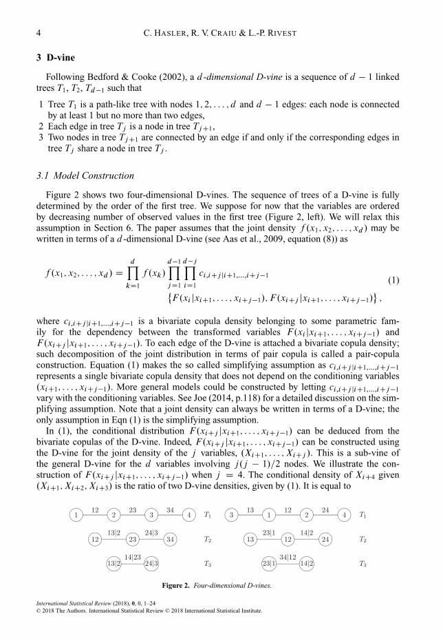
Figure 2 shows two four-dimensional D-vines. The sequence of trees of a D-vine is fullydetermined by the order of the first tree. We suppose for now that the variables are orderedby decreasing number of observed values in the first tree (Figure 2, left). We will relax thisassumption in Section 6. The paper assumes that the joint density f .x1; x2; : : : ; xd / may bewritten in terms of a d -dimensional D-vine (see Aas et al., 2009, equation (8)) as

f .x1; x2; : : : ; xd / D

dYkD1

f .xk/

d�1YjD1

d�jYiD1

ci;iCj jiC1;:::;iCj�1

®F.xi jxiC1; : : : ; xiCj�1/; F .xiCj jxiC1; : : : ; xiCj�1/

¯;

(1)

where ci;iCj jiC1;:::;iCj�1 is a bivariate copula density belonging to some parametric fam-ily for the dependency between the transformed variables F.xi jxiC1; : : : ; xiCj�1/ andF.xiCj jxiC1; : : : ; xiCj�1/. To each edge of the D-vine is attached a bivariate copula density;such decomposition of the joint distribution in terms of pair copula is called a pair-copulaconstruction. Equation (1) makes the so called simplifying assumption as ci;iCj jiC1;:::;iCj�1

represents a single bivariate copula density that does not depend on the conditioning variables.xiC1; : : : ; xiCj�1/. More general models could be constructed by letting ci;iCj jiC1;:::;iCj�1

vary with the conditioning variables. See Joe (2014, p.118) for a detailed discussion on the sim-plifying assumption. Note that a joint density can always be written in terms of a D-vine; theonly assumption in Eqn (1) is the simplifying assumption.

In (1), the conditional distribution F.xiCj jxiC1; : : : ; xiCj�1/ can be deduced from thebivariate copulas of the D-vine. Indeed, F.xiCj jxiC1; : : : ; xiCj�1/ can be constructed usingthe D-vine for the joint density of the j variables, .XiC1; : : : ; XiCj /. This is a sub-vine ofthe general D-vine for the d variables involving j.j � 1/=2 nodes. We illustrate the con-struction of F.xiCj jxiC1; : : : ; xiCj�1/ when j D 4. The conditional density of XiC4 given.XiC1; XiC2; XiC3/ is the ratio of two D-vine densities, given by (1). It is equal to

Figure 2. Four-dimensional D-vines.



f .xiC4jxiC1; xiC2; xiC3/

Df .xiC1; xiC2; xiC3; xiC4/

f .xiC1; xiC2; xiC3/

D f .xiC4/ciC3;iC4¹F.xiC3/; F .xiC4/ºciC2;iC4jiC3¹F.xiC2jxiC3/; F .xiC4jxiC3/º

ciC1;iC4jiC2;iC3¹F.xiC1jxiC2; xiC3/; F .xiC4jxiC2; xiC3/º

Df .xiC2; xiC3; xiC4/

f .xiC2; xiC3/ciC1;iC4jiC2;iC3¹F.xiC1jxiC2; xiC3/; F .xiC4jxiC2; xiC3/º

D f .xiC4jxiC2; xiC3/ciC1;iC4jiC2;iC3¹F.xiC1jxiC2; xiC3/; F .xiC4jxiC2; xiC3/º:(2)

Integrating the two sides of (2) allows to express the conditional distribution ofXiC4 in termsof CiC1;iC4jiC2;iC3, the copula distribution function, as

F.xiC4jxiC1; xiC2; xiC3/ D@CiC1;iC4jiC2;iC3 ¹F.xiC1jxiC2; xiC3/; F .xiC4jxiC2; xiC3/º

@F.xiC1jxiC2; xiC3/:

This holds for arbitrary values of j giving

F.xiCj jxiC1; : : : ; xiCj�1/

D@CiC1;iCj jiC2;:::;iCj�1

®F.xiC1jxiC2; : : : ; xiCj�1/; F .xiCj jxiC2; : : : ; xiCj�1/

¯@F.xiC1jxiC2; : : : ; xiCj�1/

:

(3)

A similar construction for the conditional distribution F.xi jxiC1; : : : ; xiCj�1/ gives

F.xi jxiC1; : : : ; xiCj�1/

D@Ci;iCj�1jiC1;:::;iCj�2

®F.xi jxiC1; : : : ; xiCj�2/; F .xiCj�1jxiC1; : : : ; xiCj�2/

¯@F.xiCj�1jxiC1; : : : ; xiCj�2/

:

(4)

These are special cases of a result first noticed by Joe (1996). Equations (3) and (4) allow thesequential evaluation of the conditional distributions appearing in (1).

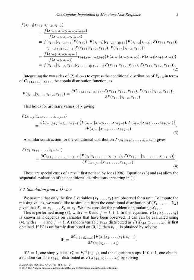
3.2 Simulation from a D-vine

We assume that only the first ` variables .x1; : : : ; x`/ are observed for a unit. To impute themissing values, we would like to simulate from the conditional distribution of .X`C1; : : : ; Xd /given that X1 D x1; : : : ; X` D x`. We first consider the problem of simulating X`C1.

This is performed using (3), with i D 0 and j D `C 1. In that equation, F.x1jx2; : : : ; x`/is known as it depends on variables that have been observed. It can can be evaluated using(4), with i D 1 and j D `. A random variable v`C1 distributed as F.X`C1jx2; : : : ; x`/ is firstobtained. If W is uniformly distributed on .0; 1/, then v`C1 is obtained by solving

W D@C1;`C1j2;:::;` ¹F.x1jx2; : : : ; x`/; v`C1º

@F.x1jx2; : : : ; x`/:

If ` D 1, one simply takes x�2 D F �12 .v`C1/, and the algorithm stops. If ` > 1, one obtains

a random variable v`C1;1 distributed as F.X`C1jx3; : : : ; x`/ by solving



v`C1 D@C2;`C1j2;:::;`

®F.x2jx3; : : : ; x`/; v`C1;1

¯@F.x2jx3; : : : ; x`/

:

If ` D 2, one simply takes x�3 D F �13 .v`C1;1/, and the algorithm stops. Note that this step

requires the evaluation of the numerical value of F.x2jx3; : : : ; x`/. It can can be evaluated using(4), with i D 2 and j D `�1. For an arbitrary value of `, this algorithm has to be iterated `�1times to obtain x�

`C1, a simulated value for variable X`C1. To simulate X`C2, one repeats thealgorithm starting at the values X1 D x1; : : : ; X` D x`; X`C1 D x�

`C1. These calculations arerelatively technical, and they can be organised efficiently; see algorithm 2 of Aas et al. (2009).We used their algorithm to simulate from our vine model.

3.3 Example: Four-dimensional Case

We first show how (3) and (4) allow the sequential evaluation of the conditional distributionsappearing in (1) when d D 4. In this case, the density becomes

f .x1; x2; x3; x4/ D f .x1/f .x2/f .x3/f .x4/

c12 ¹F.x1/; F .x2/º c23 ¹F.x2/; F .x3/º c34 ¹F.x3/; F .x4/º

c13j2 ¹F.x1jx2/; F .x3jx2/º c24j3 ¹F.x2jx3/; F .x4jx3/º

c14j23 ¹F.x1jx2; x3/; F .x4jx2; x3/º :

The first two conditional distributions F.x1jx2/ and F.x3jx2/ are obtained using (4) and (3),with i D 1 and j D 2. We obtain

F.x1jx2/ D@C12 ¹F.x1/; F .x2/º

@F.x2/;

F .x3jx2/ D@C23 ¹F.x2/; F .x3/º

@F.x2/:

The next two conditional distributions F.x2jx3/ and F.x4jx3/ are obtained using (4) and (3),with i D 2 and j D 2. We obtain

F.x2jx3/ D@C23 ¹F.x2/; F .x3/º

@F.x3/;

F .x4jx3/ D@C34 ¹F.x3/; F .x4/º

@F.x3/:

The last two conditional distributions F.x1jx2; x3/ and F.x4jx2; x3/ are obtained using (4)and (3), with i D 1 and j D 3, and the numerical values of the conditional distributionsobtained previously. We obtain

F.x1jx2; x3/ D@C13j2 ¹F.x1jx2/; F .x3jx2/º

@F.x3jx2/;

F .x4jx2; x3/ D@C24j3 ¹F.x2jx3/; F .x4jx3/º

@F.x2jx3/:

Now, we show how to simulate from the conditional distribution of the missing values giventhe observed values. With monotone non-response, there are three conditional distributions thatwe want to simulate from: .X2; X3; X4/ given X1 D x1, .X3; X4/ given X1 D x1 and X2 D x2



and X4 given X1 D x1; X2 D x2 and X3 D x3. We first consider the problem of simulating X2

given X1 D x1, X3 given X2 D x2 and X1 D x1 and X4 given X3 D x3; X2 D x2 and X1 D x1.To simulate X2 given X1 D x1, we consider (3) with i D 0 and j D 2:

F.x2jx1/ D@C12 ¹F.x1/; F .x2/º

@F.x1/:

In that equation, F.x1/ is known as it depends on a variable that has been observed. A randomvariable v2 distributed as F.X2jx1/ is first obtained. If W is uniformly distributed on .0; 1/,then v2 is obtained by solving

W D@C12 ¹F.x1/; v2º

@F.x1/:

The simulated value of X2 given X1 D x1 is x�2 D F�12 .v2/. To simulate X3 given X2 D x2

and X1 D x1, we consider (3), with i D 0 and j D 3. We obtain

F.x3jx1; x2/ D@C13j2 ¹F.x1jx2/; F .x3jx2/º

@F.x1jx2/:

In that equation, F.x1jx2/ is known, as it depends on variables that have been observed. Itcan be evaluated as shown previously. A random variable v3 distributed as F.X3jx2/ is firstobtained. If W is uniformly distributed on .0; 1/, then v3 is obtained by solving

W D@C13j2 ¹F.x1jx2/; v3º

@F.x1jx2/:

Then, one obtains a random variable v3;1 distributed as F.X3/ by solving

v3 D@C23 ¹F.x2/; v3;1º

@F.x2/:

The simulated value ofX3 givenX2 D x2 andX1 D x1 is x�3 D F�13 .v3;1/. To simulate from

X4 given X3 D x3; X2 D x2 and X1 D x1, one applies a similar construction. Three steps willbe required.

We show now how we can simulate from .X2; X3; X4/ given X1 D x1 in three steps: first,one simulates x�2 from X2 given X1 D x1; second, one simulates x�3 from X3 given X1 D x1

and X2 D x�2 ; and lastly, one simulates x�4 from X4 given X1 D x1; X2 D x�2 and X3 D x�3 .Applying the same construction, we simulate from .X3; X4/ given X1 D x1 and X2 D x2 intwo steps and from X4 given X3 D x3; X2 D x2 and X1 D x1 in one step.

4 Estimation

This section addresses the D-vine parameters estimation for a given D-vine structure andgiven pair-copula families. We apply a margin-free method and maximise an observed-datapseudo log-likelihood function. We explain how this function can be maximised using a methodto evaluate the pseudo log-likelihood function in the complete-data case. Section 4.1 presentsfirst our proposed estimation method for four variables, and in Section 4.2, we extend the ideasto the general case of d variables.



4.1 Observed-data Pseudo-likelihood for Four Variables

With complete response, the contribution of a unit to the likelihood function isf .x1; x2; x3; x4/. As assumed earlier, the missing data are MCAR. In this case, ignoring theprocess that causes missing data yields proper inference (see Rubin, 1976). When we ignore theprocess that causes missing data, we use the observed-data likelihood where the contribution tothe likelihood of a unit is

f .xobs/ D

Zf .xobs; xmis/dxmis; (5)

where xobs and xmis are the observed and missing variables of this unit, respectively. In the caseof monotone non-response, the contribution to the likelihood of a unit in s3 is

f .x1; x2; x3/ D

Zf .x1; x2; x3; x4/dx4:

By integrating the four-dimensional D-vine density in (1), we obtain

f .x1; x2; x3/ D f .x1/f .x2/f .x3/c12 ¹F.x1/; F .x2/º c23 ¹F.x2/; F .x3/º c13j2 ¹F.x1jx2/; F .x3jx2/º :

That is, the contribution to the likelihood of a unit in s3 is f .x1; x2; x3/, which is a three-dimensional D-vine density. This three-dimensional D-vine is a sub-vine of the initial four-dimensional D-vine considered. We apply recursively the same construction and obtain thecontribution to the likelihood of a unit in s2:

f .x1; x2/ D

Zf .x1; x2; x3/dx3 D f .x1/f .x2/c12 ¹F.x1/; F .x2/º ;

which is the density of a two-dimensional sub-D-vine of the initial four-dimensional D-vineconsidered. Hence, we can associate a sub-D-vine to each subsample s`. Figure 3 shows thethree sub-D-vines and the associated subsamples.

We use the margin-free semi-parametric estimation method of Genest et al. (1995) to esti-mate the copula parameters of the D-vine. The idea is to estimate the margins using empiricaldistribution functions and the copula parameters via a parametric family. We consider the con-tributions of the units in the different subsamples developed previously, and we select the copulaparameters that maximise the following observed-data pseudo log-likelihood function:

log QL.�jx1; x2; x3; x4/ DXk2s2

log ck12 CXk2s3

�log ck12 C log ck23 C log ck13j2

�

CXk2s4

�log ck12 C log ck23 C log ck34 C log ck13j2 C log ck24j3 C log ck14j23

�;

(6)where ck

i;iCj jiC1;:::;iCj�1 is a shortcut for

ci;iCj jiC1;:::;iCj�1

�F.yk;i jyk;iC1; : : : ; yk;iCj�1/; F .yk;iCj jyk;iC1; : : : ; yk;iCj�1/

�:

Here, yk;i D bF i .xk;i / and bF i is niniC1 times the empirical marginal distribution of the

i -th variable, and ni is the number of observed values of this variable. Note that when themissing data are MCAR, bF i is a consistent estimator of the marginal distribution of the



Figure 3. Monotone non-response pattern for four variables and four-dimensional D-vine with sub-D-vine associated withs2 (solid), s3 (dashed) and s4 (dotted).

i -th variable. In addition F.yk;i jyk;iC1; : : : ; yk;iCj�1/ and F.yk;iCj jyk;iC1; : : : ; yk;iCj�1/ areevaluated recursively, using (3) and (4), as functions of yk;i and of the bivariate copulas forthe sub-D-vine for variables .i; : : : ; i C j /. The observed-data pseudo log-likelihood functionin (6) can be rewritten:

log QL.�jx1; x2; x3; x4/

D logL2.�11jx1; x2/C logL3.�11;�12;�21jx1; x2; x3/C logL4.�jx1; x2; x3; x4/;(7)

where

logL2.�11jx1; x2/ DXk2s2

log ck12;

logL3.�11;�12;�21jx1; x2; x3/ DXk2s3

�log ck12 C log ck23 C log ck13j2

�;

logL4.�jx1; x2; x3; x4/ DXk2s4

�log ck12 C log ck23 C log ck34 C log ck13j2 C log ck24j3

C log ck14j23

�;

where �j i is the parameter of the copula density ci;iCj jiC1;:::;iCj�1 and � D.�11;�12;�13;�21;�22;�31/ is the parameter vector of the four-dimensional D-vine. Thefunction logL2.�11jx1; x2/ is the complete-data pseudo log-likelihood function of thetwo-dimensional sub-D-vine on x1 and x2 given the observations in s2. Similarly,logL3.�11;�12;�21jx1; x2; x3/ is the complete-data pseudo log-likelihood function of thethree-dimensional sub-D-vine on x1, x2 and x3 given the observations in s3, andlogL4.�jx1; x2; x3; x4/ is the complete-data pseudo log-likelihood function of the four-dimensional D-vine on x1, x2, x3 and x4 given the observations in s4. These three functions arecomplete-data pseudo log-likelihood functions restricted to subsamples of the initial sample.

Aas et al. (2009) propose an algorithm (algorithm 4, p. 188) to evaluate the complete-datapseudo log-likelihood function of a D-vine when there are no missing data. We apply theiralgorithm to evaluate L2, L3 and L4 in (7). We obtain an estimate of the vector parameter� by numerical maximisation of the observed-data pseudo log-likelihood function log QL. A



procedure to set the starting value of the parameters for the numerical maximisation ishighlighted in Section 5.

We should emphasise that the observed-data pseudo log-likelihood function underlying theapproach described previously is the full observed data one, and therefore, we do not expectany loss in information or statistical efficiency. The vine-induced factorisation of the pseudolog-likelihood makes the EM algorithm, commonly used in missing data problem, irrelevant forpair-copula models.

4.2 Observed-data Pseudo-likelihood for d Variables

In the d -dimensional case, the sample is partitioned into d subsamples s`, ` D 1; : : : ; d ,where s` contains those units having the first ` variables observed and the last d � ` vari-ables missing. Repeating the same construction as for four variables, we obtain the followingobserved-data pseudo log-likelihood function:

log QL.�jx1; x2; : : : ; xd / D

dX`D2

logL`.�11; : : : ;�`�1;1jx1; x2; : : : ; x`/

D

dX`D2

Xk2s`

`�1XjD1

`�jXiD1

log cki;iCj jiC1;:::;iCj�1;

(8)

where

logL`.�11; : : : ;�`�1;1jx1; x2; : : : ; x`/ DXk2s`

`�1XjD1

`�jXiD1

log cki;iCj jiC1;:::;iCj�1:

The contribution of subsample s` to the likelihood is logL`, which is the complete-datapseudo log-likelihood function of a `-dimensional D-vine for x1; x2; : : : ; x` given the observa-tions in s`. We obtain an estimate of the vector parameter � by numerical maximisation of thepseudo log-likelihood function adapted for monotone non-response log QL in (8). The algorithmof Aas et al. (2009) is applied to evaluate logL`, ` D 2; : : : ; d .

5 Selection of the Bivariate Copula Families

This section addresses the selection of the bivariate copula families given a D-vine treestructure. We apply a sequential procedure that fully uses the observed data. To select thebivariate copula families of a given D-vine, we propose a simple modification for monotonenon-response of the sequential procedure introduced in Section 6 of Aas et al. (2009). InSection 4, we have considered that the inputs of a pair-copula density ci;iCj jiC1;:::;iCj�1 areF.yk;i jyk;iC1; : : : ; yk;iCj�1/ and F.yk;iCj jyk;iC1; : : : ; yk;iCj�1/. In what follows, we willrefer to these inputs to as pseudo-observations. The general idea of our method is the following:

1B. Use a measure of quality such as Akaike Information Criterion to separately select acopula family for each pair copula ci;iC1 of the tree 1; use the largest possible set ofpseudo-observations, that is, use yk;i , yk;iC1 for k 2 siC1 [ : : : [ sd .

1C. Estimate the copula parameter of each pair copula ci;iC1 separately by maximisation ofthe pseudo log-likelihood associated

Plog cki;iC1; use the largest possible set of pseudo-

observations as in the previous step.



2A. Construct the pseudo-observations F.yk;i jyk;iC1/, F.yk;iC2jyk;iC1/ associated with thetree 2 using (3) and (4), the pseudo-observations of the previous tree and the pair-copulafamilies and parameters selected for the the previous tree.

2B. Use a measure of quality such as Akaike Information Criterion to separately select acopula family for each pair copula ci;iC2jiC1 of tree 2; use the largest possible set ofpseudo-observations, that is use F.yk;i jyk;iC1/, F.yk;iC2jyk;iC1/ for k 2 siC2[ : : :[sd .

2C. Estimate the copula parameter of each pair copula ci;iC2jiC1 separately by maximisationof the pseudo log-likelihood associated

Plog ck

i;iC2jiC1; use the largest possible set ofpseudo-observations as in the previous step.

3. Iterate for trees 3 to ` � 1.

The purpose of this sequential procedure is to select the bivariate copula families, but itsoutputs also include estimated values of the parameters. These values may be used as start-ing values of the parameters in the numerical maximisation of the observed-data pseudolog-likelihood of Section 4.

6 Tree Structure Selection

This section addresses the selection of a D-vine tree structure. Until now, we have supposedthat the variables were ordered by increasing number of observed values in the first tree (seeFigure 2, left, for the four-dimensional case). We show in this section that our estimation methodcan be applied for other D-vine tree structures and present a procedure to select such a structurefor four and d variables in Sections 6.1 and 6.2, respectively.

6.1 Selection of a Tree Structure for Four Variables

An important condition associated with the estimation method presented in Section 4 is thatthe subsamples can be associated with sub-D-vines of the initial D-vine considered. Figure 4shows two examples of D-vine tree structures having this particularity.

Figure 4. Two four-dimensional D-vine tree structures for which our estimation method can be applied. Sub-D-vinesassociated with s2 (solid), s3 (dashed) and s4 (dotted) are shown.



In the case of four variables, there are four such D-vine tree structures determined by thefollowing orders of the variables in the first tree.

Note that two symmetric trees define the same decomposition, which is the reason why welisted here four rather than eight tree structures. The idea is to select the tree structure thatmaximises the dependency accounted for in the first tree. The dependency is quantified viathe empirical Kendall’s tau. Let �ij be the empirical Kendall’s � of xi and xj , i < j . Whenestimating the Kendall’s � of data with non-response, we may want to use as many observationsas possible for efficiency purposes. In this case, we use those units that allow to compute thepairwise Kendall’s tau. Because of the non-response pattern, the different Kendall’s �s may beestimated using samples of different sizes. For instance, with monotone non-response, �12 isestimated via a sample of size n2 C n3 C n4 and �14 via a sample of size n4. As a result, �12

has less variability than �14, and we are more confident about a strong dependency betweenx1 and x2 when �12 is high than we are about a strong dependency between x1 and x4 when�14 is high. Therefore, extra care has to be taken when comparing the different Kendall’s � ’s.We describe below the proposed procedure to select a D-vine tree structure that maximises thedependency accounted for in the first tree. Our proposed procedure bypasses the problem ofdifferent variability in the �s by comparing pairs of �s that are estimated based on samples ofsame size.

1 Start with variable x1 and x2 adjacent, that is, T1 D .1; 2/.2 Compute �13 and �23 using s3[ s4. If �13 > �23, set x3 to the left of x1, that is, T1 D .3; 1; 2/.

Otherwise, set x3 to the right of x2, that is, T1 D .1; 2; 3/.3 If T1 D .3; 1; 2/, compute �34 and �24 using s4.

If �34 > �24, set x4 to the left of x3, that is, T1 D .4; 3; 1; 2/.Otherwise, set x4 to the right of x2, that is, T1 D .3; 1; 2; 4/.

Else if T1 D .1; 2; 3/, compute �14 and �34 using s4.

If �14 > �34, set x4 to the left of x1, that is, T1 D .4; 1; 2; 3/.Otherwise, set x4 to the right of x3, that is, T1 D .1; 2; 3; 4/.

Algorithm 1 Selection of a D-vine tree structure. Selects the order of the variables in the firsttree T1 of the D-vine decomposition. The Algorithm returns a vector v.d; j /, j D 1; : : : ; dwhich gives the order of the variables in the first tree.

Set v.2; 1/ D 1, v.2; 2/ D 2for i 3; : : : ; d do

Compute �v.i�1;1/;i and �v.i�1;i�1/;i usingSdkDi sk;

if �v.i�1;1/;i > �v.i�1;i�1/;i thenv.i; 1/ D i ;for j 2; : : : ; i do

v.i; j / D v.i � 1; j � 1/;end for

elsev.i; i/ D i ;for j 1; : : : ; i � 1 do

v.i; j / D v.i � 1; j /;end for

end ifend for



6.2 Selection of a D-vine Tree Structure for d Variables

We generalise the procedure applied for four variables. The estimation method of Section 4exploits the maximal amount of data possible if variables x1 to x` define a `-dimensional sub-D-vine, for ` D 2; : : : ; d . There are 2d�2 such d -dimensional D-vine tree structures (rememberthat two symmetric tree structures determine the same decomposition). Algorithm 1 presentsthe proposed procedure to select one of those.

The algorithm compares pairs of �s estimated via the same sample size to select a D-vinetree structure that maximises the dependency accounted for in the first tree. This algorithmconstructs the first tree of the D-vine sequentially. It does not require to list all possible D-vinetree structures. This may be computationally interesting in high dimensions because the numberof possible D-vine tree structures grows exponentially with the dimension.

7 Simulation Studies

7.1 Real Data

We consider the Labour Force Survey Five-Quarter Longitudinal Dataset January 2014–March 2015 (Office for National Statistics. Social Survey Division and Northern IrelandStatistics and Research Agency. Central Survey Unit, 2015). The data are distributed by theUK Data Archive at the University of Essex. We consider the total actual hours in main andsecond job (hereafter total actual hours) for five consecutive quarters as variables of interest.We denote these variables by x`, ` D 1; : : : ; 5, where the index refers to the quarter. Only sur-veyed individuals with available and non-null total actual hours for the five consecutive quartersare considered. This results in a sample of n D 1 738 individuals aged between 16 and 69. Inthis sample, the total actual hours ranges from 1 to 97. The value 97 indicates a total actualhours greater than or equal to 97. Figure 5 shows the resulting data. This plot suggests a slightasymmetry and tail dependence.

Tree structure and pair-copulas families When applied to the complete data (1,738 obser-vations), Algorithm 1 selects the D-vine tree structure that agrees with time order. That is, thevariables are ordered by time in the first tree of the D-vine. We also conduct 1,000 simulationsto study the impact of non-response on the selected tree structure. For each simulation run, werandomly generate a monotone non-response pattern as follows: we randomly partition the unitsinto five subsamples s1; s2; : : : ; s5 of approximately equal size; for a unit k 2 s`, ` D 1; 2; : : : ; 5,we discard the values xki for i > `. Note that the missing data are MCAR. For each incom-plete data generated, we apply Algorithm 1 and select a D-vine tree structure. Table 1 showsthe selected tree structures with the frequency of occurrence across 1,000 simulations.

Only 5 out of the 16 possible tree structures are observed. The tree with the variables orderedby time is selected for almost 75% of the simulation runs. The other four selected tree structuresare very close to the first one. First, the orders are very similar. For instance, the order of the firsttwo tree structures is the same except for the fifth variable. Second, the strength of dependencyaccounted for in the first tree is very similar across the five selected tree structures. Indeed,the average Kendall’s � of the pairs in the first tree for these five tree structures computed onthe complete data ranges from 0.578 (fifth tree structure) to 0.593 (first tree structure). As aresult, there would be almost no difference in terms of accuracy and stability of the parametersestimators between these five tree structures. We consider the D-vine with the variables orderedby time in the first tree in what follows.

We apply the procedure of Section 5 to the complete data to select the pair-copula familiesof the D-vine. We obtain survival Gumbel family for pairs 1, 2, 4 and 10, Gumbel family for



Figure 5. Total actual hours of 1 738 individuals for five consecutive quarters.

Table 1. Frequency of the ordersselected with Algorithm 1 for thetotal actual hours of 1 738 indi-viduals for five consecutive quar-ters over 1 000 simulations.

Order Frequency

1 - 2 - 3 - 4 - 5 0.735 - 1 - 2 - 3 - 4 0.205 - 4 - 1 - 2 - 3 0.035 - 4 - 3 - 1 - 2 0.034 - 1 - 2 - 3 - 5 <0.01



pairs 3, 5, 6, 7 and 9 and Frank family for pair 8. This confirms the presence of asymmetry andtail dependence that we have graphically observed.

Imputation We conduct 200 simulations to compare the performance of our method to othermethods. For each simulation run, we randomly generate a monotone non-response pattern asdescribed previously. For each simulation run, we impute the missing data using six imputationmethods:

1. MEan IMPutation (MEIMP) The missing values of each variable are replaced with themean of this variable.

2. AMElia (AME)(Honaker et al., 2011) The algorithm runs an EM algorithm on each of mul-tiple bootstrapped samples selected from the incomplete data. Then, it draws a set of imputedvalues from the parameters estimated from each bootstrap sample (multiple imputation). Weselect five bootstrap samples. Amelia assumes a multivariate normal distribution. We applyfunction boxcox of R package Mass (Venables & Ripley, 2002) to check whether a Box–Coxpower transformation should be used to achieve normality. The selected parameters of theBox–Cox transformation being close to 1, we use the original untransformed data.

3. Multivariate Imputation by Chained Equations (MICE)(van Buuren & Groothuis-Oud-shoorn, 2011) MICE imputes the data by chained equations. It assumes an imputation modelseparately for each column in the data. For continuous variable, it applies predictive meanmatching cyclicly. The idea of predictive matching is the following: (i) it fits a linear modelwith the variable being imputed as dependent variable and some fully observed covariates;(ii) it predicts the missing values of the variable being imputed using the fitted model; and(iii) it imputes a missing value with the observed value of the variable being imputed that isthe closest to the fitted value. MICE starts with an initial imputation of each variable. Then,it cyclicly imputes each variable with predictive mean matching with the other variables(observed and imputed values) as covariates until a convergence criterion is reached. Finally,the algorithm generates multiple imputations for incomplete multivariate data by Gibbs sam-pling. We consider five multiple imputations. With continuous variables, MICE assumesnormality of the variables. We use here the original untransformed data (same reason as forAME).

4. Copula IMPutation (COIMP)(Di Lascio and Giannerini, 2014; Di Lascio et al., 2015)COIMP is a copula-based method to impute multivariate missing data. Four steps of themethod are as follows: (i) non-parametric estimation of the margins through local polyno-mial likelihood and parametric estimation of the copula model through maximum likelihoodon the available data; (ii) derivation of the joint distribution; (iii) derivation of the conditionaldistribution of the missing values, conditioned on the observed values; and (iv) imputation bygenerating from the conditional distribution of the previous step with the Hit or Miss MonteCarlo method. The copula models allowed are normal, Frank, Clayton and Gumbel. Notethat this method is the slowest among the five considered. For Labour Force Survey data, thenormal copula model is selected (for both the complete data and data with non-response) andkept constant throughout the simulations. We carry out five repeated imputations (multipleimputation).

5. Nearest Neighbor imputation (NN) We use function impute.NN_HD of R package Hot-DeckImputation (Joenssen, 2015). Function impute.NN_HD finds the nearest neighbor inthe complete cases for each case with missing values using the observed values of this case.The Manhattan distance is considered. The variables are scaled with respect to their rangeprior to computing the distance.

6. Pair-copula Imputation (PCI) We consider the D-vine with the variables ordered by timein the first tree and the pair-copulas families selected from the complete data (see previous



paragraph). We keep them constant throughout the simulations so that we can study the effectof imputing solely on the estimates. For each simulation run, we estimate the pair-copulaparameters using the procedure described in Section 4, and we sample imputed values fromthe conditional distribution of the missing values, conditioned on the observed values usingthe procedure described in Section 3.2. We carry out five repeated imputations (multipleimputation). We transform the variables back to the original scale using the inverse of thefunctions bF i described in Section 4.1.

For each imputation method and each simulation run, we estimate three vectors of parametersof interest: (i) the mean of each variable, (ii) the Pearson’s correlation of each pair of variablesand (iii) the 99th percentile of each variable. Appendix S1 explains how to compute point andvariance estimates with multiple imputation. Consider Q.i/ the point estimate obtained at thei -th simulation run for a given imputation method and a generic vector of parameters of interestQ. We assess the performance of the imputation methods via three criteria:

1. The Monte Carlo relative bias (in absolute value) defined as

RB DjBj

Q;

where B D Q.I /�Q is the Monte Carlo bias andQ

.I /DPIiD1Q

.i/=I is the average pointestimate over the I D 200 simulations.

2. The Monte Carlo relative root variance (or relative standard deviation) defined as

RRV DV1=2

Q;

where

V D1

I � 1

IXiD1

�Q.i/ �Q

.I /�2:

3. The Monte Carlo relative root mean square error defined as

RRMSE D

�B2 C VAR

�1=2

Q:

Figure 6 shows the results.The top plots show three comparison criteria for the mean of the variables ordered by decreas-

ing number of observed values, the middle plots three comparison criteria for the Pearson’scorrelation coefficient of the pairs of the variables ordered by decreasing number of pairwiseobserved values and the bottom plots three comparison criteria for the 99th percentile of thevariables ordered by decreasing number of observed values. Appendix S2 contains three tablesshowing these results. We observe that PCI is associated with smallest variance in all consideredcases considered except one. A possible explanation is that our estimation method (Section 4)uses all the information in the data. We discuss the bias associated with the six imputation meth-ods independently for each parameter of interest. For the mean, all five methods are associatedwith an RB less than 3%. MEIMP, AMEL, MICE and NN yield the smallest RB. The reason isthat the mean is a measure of central tendency, which is unrelated to the dependence and tailsstructure. Therefore, an imputation method that imputes each variable separately (MEIMP),



Figure 6. Three comparison criteria (from left to right: RB, RRV and RRMSE) for three parameters of interest (from top tobottom: mean, Pearson’s correlation coefficient and 99th percentile) with six imputation methods for Labour Force Surveydata. The x-axis shows the index of the variables or pair of variables for Pearson’s correlation coefficient. RB, relative bias;RRV, relative root variance; RRMSE, relative root mean square error.

independently to the dependence structure (MEIMP) and the tails features (MEIMP, AMEL,MICE and NN) provides satisfactory results. COIMP shows the poorest performance; it is alsothe slowest. For the Pearson’s correlation coefficient, AMEL, MICE, NN and PCI yield thesmallest RB. This was expected because these four imputation methods account for the depen-dence structure of the data. For this parameter of interest, MEIMP and COIMP yield an RBthat can be as high as nearly 60% and 80%, respectively. For MEIMP, the reason is that it doesnot account for the dependence structure as the variables are imputed separately. The bad per-formance of COIMP, however, is surprising because this method accounts for the dependencestructure via a copula model. A possible explanation is that the family of copulas used by thismethod is not wide enough to capture the dependence structure of the data. For the 99th per-centile, PCI globally provides the best results. The reason is that this method accounts for thetails features.

7.2 Simulated Data 1

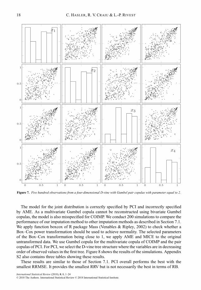
We simulated a sample of size n D 500 from a four-dimensional D-vine with Gumbel paircopulas with parameter equal to 2. Figure 7 shows the simulated data.



Figure 7. Five hundred observations from a four-dimensional D-vine with Gumbel pair copulas with parameter equal to 2.

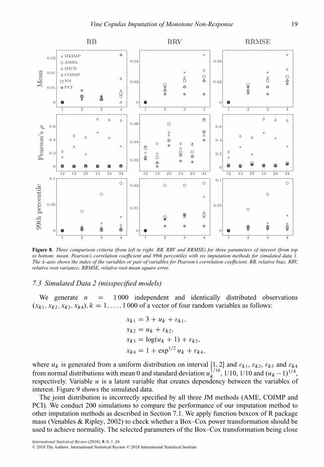
The model for the joint distribution is correctly specified by PCI and incorrectly specifiedby AME. As a multivariate Gumbel copula cannot be reconstructed using bivariate Gumbelcopulas, the model is also misspecified for COIMP. We conduct 200 simulations to compare theperformance of our imputation method to other imputation methods as described in Section 7.1.We apply function boxcox of R package Mass (Venables & Ripley, 2002) to check whether aBox–Cox power transformation should be used to achieve normality. The selected parametersof the Box–Cox transformation being close to 1, we apply AME and MICE to the originaluntransformed data. We use Gumbel copula for the multivariate copula of COIMP and the paircopulas of PCI. For PCI, we select the D-vine tree structure where the variables are in decreasingorder of observed values in the first tree. Figure 8 shows the results of the simulations. AppendixS2 also contains three tables showing these results.

These results are similar to those of Section 7.1. PCI overall performs the best with thesmallest RRMSE. It provides the smallest RRV but is not necessarily the best in terms of RB.



Figure 8. Three comparison criteria (from left to right: RB, RRV and RRMSE) for three parameters of interest (from topto bottom: mean, Pearson’s correlation coefficient and 99th percentile) with six imputation methods for simulated data 1.The x-axis shows the index of the variables or pair of variables for Pearson’s correlation coefficient. RB, relative bias; RRV,relative root variance; RRMSE, relative root mean square error.

7.3 Simulated Data 2 (misspecified models)

We generate n D 1 000 independent and identically distributed observations.xk1; xk2; xk3; xk4/; k D 1; : : : ; 1 000 of a vector of four random variables as follows:

xk1 D 3C uk C "k1;

xk2 D uk C "k2;

xk3 D log.uk C 1/C "k3;

xk4 D 1C exp1=2 uk C "k4;

where uk is generated from a uniform distribution on interval Œ1; 2� and "k1, "k2, "k3 and "k4

from normal distributions with mean 0 and standard deviation u1=10k

, 1/10, 1/10 and .uk�1/1=4,respectively. Variable u is a latent variable that creates dependency between the variables ofinterest. Figure 9 shows the simulated data.

The joint distribution is incorrectly specified by all three JM methods (AME, COIMP andPCI). We conduct 200 simulations to compare the performance of our imputation method toother imputation methods as described in Section 7.1. We apply function boxcox of R packagemass (Venables & Ripley, 2002) to check whether a Box–Cox power transformation should beused to achieve normality. The selected parameters of the Box–Cox transformation being close



Figure 9. One thousand independent and identically distributed observations.

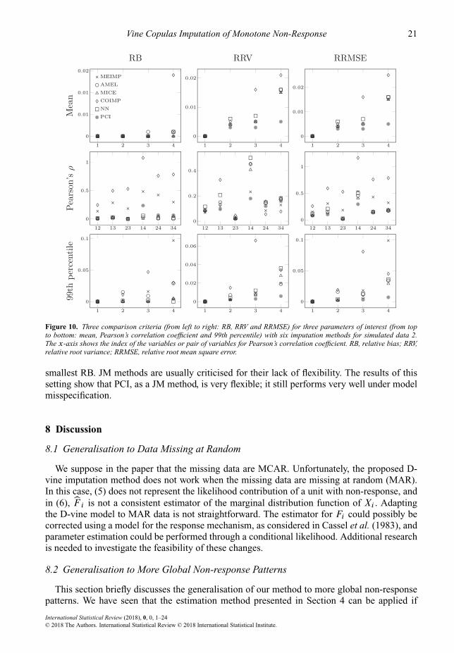
to 1, we apply AME and MICE to the original untransformed data. For COIMP, we use thecomplete data to select the copula families. We obtain the normal copula and consider this oneacross the 200 simulations. For PCI, we transform the variables as described in Section 7.1 toobtain uniform margins. We use the complete data to select the pair-copula families and theD-vine tree structure. We obtain the D-vine tree structure where the variables are in decreasingorder of observed values in the first tree. We obtain Frank copula for pairs 1, 2, 3 and 5 andindependence copula for pairs 4 and 6. We consider this D-vine tree structure and these pair-copula families across the 200 simulations. Figure 10 shows the results of the simulations.Appendix S2 also contains three tables showing these results.

Pair-copula imputation overall performs the best with the smallest RRMSE for all threeparameters of interest. For two parameters of interest (mean and 99th percentile), PCI, NN andMICE perform equally and better than the other methods in terms of RB, and PCI performs thebest in terms of RRV. For the Pearson’s correlation coefficient, AMEL, MICE and NN yield the



Figure 10. Three comparison criteria (from left to right: RB, RRV and RRMSE) for three parameters of interest (from topto bottom: mean, Pearson’s correlation coefficient and 99th percentile) with six imputation methods for simulated data 2.The x-axis shows the index of the variables or pair of variables for Pearson’s correlation coefficient. RB, relative bias; RRV,relative root variance; RRMSE, relative root mean square error.

smallest RB. JM methods are usually criticised for their lack of flexibility. The results of thissetting show that PCI, as a JM method, is very flexible; it still performs very well under modelmisspecification.

8 Discussion

8.1 Generalisation to Data Missing at Random

We suppose in the paper that the missing data are MCAR. Unfortunately, the proposed D-vine imputation method does not work when the missing data are missing at random (MAR).In this case, (5) does not represent the likelihood contribution of a unit with non-response, andin (6), bF i is not a consistent estimator of the marginal distribution function of Xi . Adaptingthe D-vine model to MAR data is not straightforward. The estimator for Fi could possibly becorrected using a model for the response mechanism, as considered in Cassel et al. (1983), andparameter estimation could be performed through a conditional likelihood. Additional researchis needed to investigate the feasibility of these changes.

8.2 Generalisation to More Global Non-response Patterns

This section briefly discusses the generalisation of our method to more global non-responsepatterns. We have seen that the estimation method presented in Section 4 can be applied if



and only if any group of variables that are jointly observed in the sample defines a sub-D-vine of the original D-vine. More generally, our method can be applied if we observe only nondiscontinuous sequences of variables, that is, if it is possible to rearrange the variables suchthat, for each unit k, there exist two scalars `� and `C such that 1 � `� < `C � d and xki isobserved for `� � i � `C and missing for i < `� or i > `C. In this case, the sample can bepartitioned into d.d � 1/=2 subsamples:

s`�;`C D®kjxki is observed if and only if `� � i � `C

¯;

where `� D 1; : : : ; d � 1, `C D `� C 1; : : : ; d . Figure 11 shows the non-response patternsfor which our estimation method can be applied and the sub-D-vines associated in the four-dimensional case.

In dimension d , there are therefore d.d � 1/=2 non-response patterns that our method canhandle. Note that our estimation method presented in Section 4 and imputation methods inSection 3.2 might need to be adapted to suit the non-response patterns presented in this section.

So far, we have considered that all variables are observed for some units (subsample s14 inthe four-dimensional case). Consider now that we jointly observe at most p < d variables inthe sample. A typical example is a longitudinal study with a cyclical selection: once a unit issampled, it is retained for exactly p consecutive waves. In this case, the sample provides no

Figure 11. Non-response patterns for which our estimation method can be applied (left) and sub-D-vines associated (right)in the four-dimensional case.

Figure 12. Non-response pattern when units are retained for three consecutive waves in the four-dimensional case, truncatedtree at level 2 and D-vines associated with the subsamples.



information about the pair copulas in the trees p to d � 1. A solution to apply our method isto set all pair copulas in trees p and higher to independence copulas. This implies a truncatedtree at level p � 1 (Brechmann et al., 2012). Figure 12 shows an example where the unitsare retained for three consecutive waves (p D 3) in the four-dimensional case. In this case,the sample provides no information about the pair copula C14j23 of Tree T3 because we neverobserve jointly all four variables. This pair is set to independence copula, which results in atruncated tree at level 2. Each subsample is associated with a D-vine, and our method can beapplied.

9 Conclusion

The paper proposes an imputation method for continuous variables based on vine copulasthat yields a flexible joint model using a cascade of bivariate copulas. Our method can capturesome complex features of the data such as tail dependence that other methods fail to capture,and it does not restrict the marginals to belong to preset families. We suppose MCAR dataand a monotone non-response pattern, and, in this case, our proposed method outperforms allcompeting alternatives. It would be interesting to generalise our method to MAR data andnon-monotone non-response patterns.

Acknowledgements

This research is supported by the Canadian Statistical Sciences Institute and by NSERC ofCanada. The authors thank a reviewer, the Editor and Pr. Harry Joe for constructive comments.

Supporting Information

Additional supporting information may be found online in the supporting information tab forthis article.

References

Aas, K., Czado, C., Frigessi, A. & Bakken, H. (2009). Pair-copula constructions of multiple dependence. Insur. Math.Econ., 44, 182–198.

Bedford, T. & Cooke, R. M. (2002). A new graphical model for dependent random variables. Ann. Statist., 30(4),1031–1068.

Brechmann, E. C., Czado, C. & Aas, K. (2012). Truncated regular vines in high dimensions with application tofinancial data. Can. J. Stat., 40(40), 68–85.

Cassel, C. M., Särndal, C.-E. & Wretman, J. H. (1983). Some uses of statistical models in connexion with the nonre-sponse problem. In Incomplete Data in Sample Surveys, Vol. 3, Eds. W. G. Madow & I. Olkin, pp. 143–160. NewYork: Academic Press.

Chauvet, G. & Haziza, D. (2012). Fully efficient estimation of coefficients of correlation in the presence of imputedsurvey data. Can. J. Stat., 40(1), 124–149.

Di Lascio, F. M. L. & Giannerini, S. (2014). CoImp: Copula based imputation method. R package version 0.2-3.Di Lascio, F. M. L., Giannerini, S. & Reale, A. (2015). Exploring copulas for the imputation of complex dependent

data. Stat. Methods Appl., 24(1), 159–175.Ding, W. & Song, P. X. -K. (2016). EM algorithm in Gaussian copula with missing data. Comput. Stat. Data Anal.,

101, 1–11.Gelman, A. & Hill, J. (2011). Opening windows to the black box. J. Stat. Softw., 40(3), 1–25.Genest, C., Ghoudi, K. & Rivest, L.-P. (1995). A semiparametric estimation procedure of dependence parameters in

multivariate families of distributions. Biometrika, 82(3), 543–552.Harrell, Jr, F. E. with contributions from Charles Dupont and many others. (2016). Hmisc: Harrell Miscellaneous. R

package version 3.17-2.



Honaker, J., King, G. & Blackwell, M. (2011). Amelia II: A program for missing data. J. Stat. Softw., 45(7), 1–47.Joe, H. (1996). Families ofm-variate distributions with given margins andm.m� 1/=2 bivariate dependence param-

eters. In Distributions with Fixed Marginals and Related Topics, Eds. L. Rueschendorf, B. Schweizer & M. Taylor,pp. 120–141. Hayward, CA, IMS Lecture Notes-Monograph Series.

Joe, H. (2014). Dependence Modeling with Copulas. Boca Raton, FL: Chapman and Hall/CRC.Joenssen, D. W. (2015). HotDeckImputation: Hot deck imputation methods for missing data. R package version 1.1.0.Käärik, E. & Käärik, M. (2009). Modeling dropouts by conditional distribution, a copula-based approach. J. Stat.

Plan. Infer., 139, 3830–3835.Office for National Statistics. Social Survey Division and Northern Ireland Statistics and Research Agency. Central

Survey Unit. (2015). Labour force survey five-quarter longitudinal dataset. january 2014 - march 2015. 2nd edition.Colchester, Essex: UK Data Archive [distributor].

Raghunathan, T. E., Lepkowski, J. M., van Hoewyk, J. & Solenberger, P. (2001). A multivariate technique for multiplyimputing missing values using a sequence of regression models. Survey Methodology, 27(1), 85–95.

Rubin, D. B. (1976). Inference and missing data. Biometrika, 63, 581–592.Rubin, D. B. (1987). Multiple Imputation for Nonreponse in Surveys. New York: Wiley.Schafer, J. L. (1997). Analysis of Incomplete Multivariate Data. London: Chapman and Hall.van Buuren, S. (2007). Multiple imputation of discrete and continuous data by fully conditional specification. Stat.

Methods Med. Res., 16(3), 219–242.van Buuren, S. & Groothuis-Oudshoorn, K. (2011). MICE: Multivariate imputation by chained equations in R. J. Stat.

Softw., 45(3), 1–67.Venables, W. N. & Ripley, B. D. (2002). Modern Applied Statistics with S, 4th ed. New York: Springer. ISBN 0-387-

95457-0.

[Received July 2016, accepted February 2018]


vine copulas for imputation of monotone non-response2011) implemented in r package mice, and the...

Documents