The University of MaineDigitalCommons@UMaine

Electronic Theses and Dissertations Fogler Library

Summer 8-18-2017

Oyster Aquaculture Site Selection Using Landsat8-derived Sea Surface Temperature, Turbidity, andChlorophyll a.Jordan SnyderUniversity of Maine, Orono, jordan.snyder@maine.edu

Follow this and additional works at: http://digitalcommons.library.umaine.edu/etd

Part of the Oceanography Commons

This Open-Access Thesis is brought to you for free and open access by DigitalCommons@UMaine. It has been accepted for inclusion in ElectronicTheses and Dissertations by an authorized administrator of DigitalCommons@UMaine. For more information, please contactum.library.technical.services@maine.edu.

Recommended CitationSnyder, Jordan, "Oyster Aquaculture Site Selection Using Landsat 8-derived Sea Surface Temperature, Turbidity, and Chlorophyll a."(2017). Electronic Theses and Dissertations. 2722.http://digitalcommons.library.umaine.edu/etd/2722

OYSTERAQUACULTURESITESELECTIONUSINGLANDSAT8–DERIVED

SEASURFACETEMPERATURE,TURBIDITY,ANDCHLOROPHYLLA

By

JordanSnyder

B.S.UniversityofCalifornia,Davis,2013

ATHESIS

SubmittedinPartialFulfillmentofthe

RequirementsfortheDegreeof

MasterofScience

(inOceanography)

TheGraduateSchool

TheUniversityofMaine

August2017

AdvisoryCommittee:

EmmanuelBoss,ProfessorofMarineScience,CoAdvisor

DamianBrady,AssistantProfessorofMarineScience,CoAdvisor

AndrewThomas,ProfessorofMarineScience

ii

Copyright2017JordanSnyder

OYSTERAQUACULTURESITESELECTIONUSINGLANDSAT8-DERIVED

SEASURFACETEMPERATURE,TURBIDITY,ANDCHLOROPHYLLA

ByJordanSnyder

ThesisAdvisors:Dr.EmmanuelBoss,DamianBrady

AnAbstractoftheThesisPresented

inPartialFulfillmentoftheRequirementsfortheDegreeofMasterofScience

(inOceanography)

August2017

Remote sensing data is useful for selection of aquaculture sites because it can providewater-quality

productsmappedwithnocosttousers.However,thespatialresolutionofmostoceancolorsatellitesis

toocoarsetoprovideusabledatawithinmanyestuaries.ThemorerecentlylaunchedLandsat8satellite

hasboththespatialresolutionandthenecessarysignaltonoiseratiotoprovidetemperature,aswellas

oceancolorderivedproductsalongcomplexcoastlines.ThestateofMaine(USA)hasanabundanceof

estuarine indentations (~3,500miles of tidal shoreline within 220miles of coast), and an expanding

aquaculture industry,whichmakes itaprimecase-study forusingLandsat8data toprovideproducts

suitable foraquaculturesite selection.Wecollected theLandsat8 scenesovercoastalMaine, flagged

clouds,atmosphericallycorrectedthetop-of-the-atmosphereradiances,andderivedtimevaryingfields

(repeattimeofLandsat8is16days)oftemperature(100mresolution),turbidity(30mresolution),and

chlorophyll-a (30 m resolution). We validated the remote-sensing-based products at several in situ

locationsalongtheMainecoastwheremonitoringbuoysandprogramsareinplace.Initialanalysisofthe

validated fields revealed promising areas for oyster aquaculture. The approach used and the data

collectedtodateshowpotentialforotherapplicationsinmarinecoastalenvironments,includingwater

qualitymonitoringandecosystemmanagement.

iii

ACKNOWLEDGEMENTS

ThankyouEmmanuelBoss,DamianBrady,AndyThomasandCarterNewellforguidingandinstructing

me.ThankyouRyanWeatherbeeforpatientlyworkingwithmeandhelpingmewiththesatellitedata

processing. Thank you to Catherine Coupland, Nicolas DelPrete, TiegaMartin, Chris Rigaud,Matthew

Grey,andRobbieDownsforyourassistancemaintainingtheLOBObuoysattheDarlingMarineCenter.

Thank you to Nils Haëntjens for assistance with data processing and editing. Thank you to Jocelyn

RunnebaumandKevinStaples for thehelpfuledits. Thankyou to theSEANETprojectatUniversityof

MaineforprovidingLOBObuoydataandtravelsupport.ThankyouDanaMorse,BethBissonandMaura

Thomasforsupport.ThankyouKelly,LeAnnandAliforbeingspectacularlabmates,andthankyoutomy

familyforyourcontinuedencouragement.

iv

TABLEOFCONTENTS

ACKNOWLEDGEMENTS...............................................................................................................................iii

LISTOFTABLES............................................................................................................................................viLISTOFFIGURES.........................................................................................................................................viiLISTOFEQUATIONS....................................................................................................................................ixLISTOFABBREVIATIONS...............................................................................................................................xChapter1.INTRODUCTION.....................................................................................................................................12. METHODS…………………………….………………………………………………………………………………………………………….6 2.1StudyArea…................................................................................................................................6 2.2ProcessingofSeaSurfaceTemperature.....................................................................................7

2.3OceanColor.................................................................................................................................9 2.4AtmosphericCorrectionfor𝑅"#................................................................................................10 2.5RetrievalofTurbidity................................................................................................................11 2.6RetrievalofChlorophyll-a..........................................................................................................11 2.7Validationwithinsitudata……..................................................................................................12 2.8SatelliteImageryforanOysterSuitabilityIndex………………………………………………………..………....13

3. RESULTS……………….............................................................................................................................15 3.1Satelliteretrievedvalidationwithinsitudata...........................................................................15 3.2SatelliteImageryforOysterGrowthConditions........................................................................204.DISCUSSION………....................................................................................................................................22

4.1SatelliteImagery…….................................................................................................................22 4.2LimitationsinValidationProcess…………………....……………………………………………………………………22

v

4.3OysterSuitabilityIndex……………………………......……………………………………………………………………….244.4FutureWork……………………………………….....……………………………………………………………………………..25

5.CONCLUSION……....................................................................................................................................27REFERENCES...............................................................................................................................................28APPENDICES...............................................................................................................................................34

AppendixA.AssessmentofAtmosphericCorrection......................................................................34AppendixB.OysterSuitabilityIndex...............................................................................................37AppendixC.AveragedMonthlySatelliteData………........................................................................38AppendixD.StandardDeviationofMonthlyClimatologyMaps…..................................................41

BIOGRAPHYOFTHEAUTHOR.....................................................................................................................44

vi

LISTOFTABLES

TableA.1. MeasuredValuesinHumicPond............................................................................34

TableA.2. ValuesfromliteratureforequationA(1)................................................................35

TableA.3. DilutionseriesofArizonaDuststandardwithHachandLOBOWQMturbidity

measurements........................................................................................................35

TableB.1.CriteriaforOysterSuitabilityIndex….....................................................................37

TableB.2.OysterSuitabilityIndexscoresandaverageJulySSTatexistingandprospectiveoyster

aquaculturesitesinMaine.........................................................................................................…37

vii

LISTOFFIGURES

Figure1. Mapofmid-coastMaine,USA...................................................................................7

Figure2. Landsat8-derivedSeasurfacetemperaturemapofmid-coastMaineon

July14,2013............................................................................................................15

Figure3. TypeIIlinearregressionformatch-upsbetweenLandsat8seasurface

temperatureandseasurfacetemperaturemeasuredbyoceanographicbuoys…..16

Figure4. Landsat8-derivedturbidityalongmid-coastMaineonJuly14,2013.....................17

Figure5. TypeIIlinearregressionbetweenLandsat8turbidityandturbiditymeasured

byLOBObuoys........................................................................................................18

Figure6. Landsat8-derivedchlorophyll-aalongmid-coastMaineonJuly14,2013..............19

Figure7. TypeIIlinearregressionbetweenLandsat8chlorophyll-aandchlorophyll-a

measuredbyLOBObuoys.......................................................................................20

Figure8. Oystersuitabilitymapbasedonphysicaloceanographicparameters:

seasurfacetemperature,turbidity,andchlorophyll-a............................................21

FigureA.1. TypeIIlinearregressionbetweenLandsat8chlorophyll-aandchlorophyll-a

measuredbyLOBObuoysatnighttime..................................................................36

FigureC.1. SeasurfacetemperaturederivedfromLandsat8dataaveragedoverall

imagesinJulyfrom2013to2016.…….....................................................................38

FigureC.2. TurbidityderivedfromLandsat8dataaveragedoverallimagesinJuly

from2013to2016.…….............................................................................................39

FigureC.3. Chlorophyll-aderivedfromLandsat8dataaveragedovereachimageinJuly

from2013to2016.……............................................................................................40

FigureD.1. StandarddeviationofmonthlyaveragedseasurfacetemperaturedatainJuly

from2013to2016…................................................................................................41

viii

FigureD.2. StandarddeviationofmonthlyaveragedturbiditydatainJulyfrom

2013to2016….........................................................................................................42

FigureD.3. Standarddeviationofmonthlyaveragedchlorophyll-adatainJulyfrom

2013to2016….........................................................................................................43

ix

LISTOFEQUATIONS

Equation1. Retrievalofturbiditywithremotesensingreflectance....................................................11

Equation2. Retrievalofchlorophyll-awithOC3……………….................................................................11

Equation3. CalculationofOysterSuitabilityIndex………………………………………………………………………….14

EquationA.1. Relationshipbetween𝑅"#andabsorptionandbackscatteringcoefficients………………….34

x

LISTOFABBREVIATIONS

SST-SeaSurfaceTemperature

T–Turbidity

SPM–SuspendedParticulateMatter

Chla–Chlorophyll-a

AVHRR–AdvancedVeryHighResolutionRadiometer

𝑅"#–Remotesensingreflectance

OSI–OysterSuitabilityIndex

DRE–DamariscottaRiverEstuary

CDOM–coloreddissolvedorganicmatter

NERACOOS–NortheasternRegionalAssociationofCoastalOceanObservingSystems

LOBO–Land/OceanBiogeochemicalObservatory

NTU–Nephalometricturbidityunits

𝑏–backscattering

𝑏%&–backscatteringofparticles

𝑏%'–backscatteringofwater

𝑎'–absorptionofwater

𝑎&∗–absorptionofparticles

𝑎*–absorptionofdissolvedsubstances

1

CHAPTER 1

INTRODUCTION

Oyster aquaculture of the American oyster,Crassostrea virginica, is an expanding industry in coastal

Maine,USA,withlandingsworth$4.8milliondollarsin2015,upfrom$0.6millionin2003andincreasing

by250%between2011and2015(MaineDMRcommerciallandings2016,www.maine.gov/dmr).Tomeet

thegrowingdemandforhighqualityoysters,identificationofnewsiteswiththemostoptimalbiophysical

conditionsforoystergrowthisneeded.Todecreasetheriskofchoosinganunproductivesite,itiscrucial

thatgrowershavetherighttoolsforsiteselection.Currently,themethodforselectingasuitablesitefor

bivalveaquacultureislargelybasedonproximitytoexistingsitesortrialanderror.Thesemethodsare

inefficientbecausetheymaynotconsiderthespecifictemperatureandnutritionalconditionsneededfor

thespeciestogrow,eachofwhichaffecthowfast it takestoreachmarketsize(Hawkinsetal.,2013;

Rheault&Rice,1996).Recentadvancesinremotesensingtechniquesenablesatelliteimagerytohelpin

site selection (e.g. Thomas et al., 2011). By visually inspecting information products calculated from

processedLandsat8satellite images,estuaries that reachrelativelywarmtemperatures (above20°C),

supporthighlevelsofchlorophyllinthesummer(above1μgChlL-1),andexhibitlowturbidity(below8

NTU)canbeefficientlyidentifiedaspotentialoystergrowingareas.

Thespatialresolutionofstandardglobaloceancolorsatellites(typically1kmx1km)istoocoarse

toprovideusabledatawithinthemanyestuariesandembaymentsalongcoastalMainewheremuchof

the suitable habitat for oyster aquaculture is located. The Thermal Infrared Sensor (TIRS) and the

OperationalLandImager(OLI)aresensorsontheLandsat8satellite,launchedFebruary11,2013.These

sensorshaveboththespatialresolution(100mforinfrareddataand30mformultispectralvisibledata)

and the necessary signal to noise ratio to provide useful temperature aswell as ocean color derived

products along the Maine coastline (Vanhellemont and Ruddick, 2014). In this paper, we used a

2

combination of empirical and analytical approaches to derive temperature, turbidity and chlorophyll

productsfromLandsat8OperationalLandImager(OLI)andThermalInfraredSensor(TIRS)dataforthe

coastofMaine.

Although it was designed for terrestrial monitoring, Landsat 8 data can be used for marine

applications ifa reliableatmospheric correction isapplied.Anatmospheric correction isnecessary for

satelliteremotesensingbecauseinthevisiblewavelengthsthesignalobservedbythesatelliteisreflected

from gas and aerosol particles in the atmosphere (Mobley et al, 2016).We used theNASA software

platformSeaDAS,andalgorithmsimplementedwithinit,togetherwithanempiricalapproachtoderive

chlorophyllandturbidity.

Aswithanyinstrument,therearelimitationstousingLandsat8imageryforcoastalmonitoring.

Comparedtosatellites,suchasAVHRRandMODIS,thathavedailycoverage,thetemporalresolutionof

Landsat8coverageislow.The16dayrepeatcoveragemakesitinsufficienttoobserveshort-termchanges

(duetoweather,stormevents,etc.),butit isusefulfordescribingpatternssuchasseasonalaverages,

whichisinformativeformonitoringlong-termconditionsandrelativespatialdifferencesbetweensites.

Additionally,cloudcoverdecreasestheprobabilityofclearoverpasses;mostoftheimagesweretrieved

comefromsummerandfallmonths(JunethroughNovember)whentherewastheleastamountofcloud

cover.Fortunately,thisisalsothecriticaltimeofyearforoysteraquacultureasitoverlapsmostofthe

growingseason.

Ocean color measurements can be used to describe components of water quality, such as

turbidityandchlorophyll-a(Chla)concentration(O’Reillyetal.,1998).Algorithmshavebeendeveloped

that can estimate concentrations of these components by 1) retrieving radiant flux from the target

surface,2)correctingforthesignalfromtheatmosphere,3)transformingradiantenergycollectedbythe

satellite sensor into remote sensing reflectance (R,-), and 4) converting R,- values into products.

3

Reflectanceintheredwavelengthsoflightisusedtoestimatesuspendedparticulatematter(Dogliottiet

al.,2015;VanhellemontandRuddick,2014),whilereflectanceintheblueandgreenwavelengthsisused

toestimateofChlabiomass(aproxyofphytoplanktonbiomass)(Franzetal.,2015;Mobleyetal.,2016).

Thesemethodshavebeenusedformonitoringinseveralsitesaroundtheworld(Aguilar-Manjarrezand

Crespi,2013;Gernezetal.,2014;Radiartaetal.,2008;Thomasetal.,2011;Wangetal.,2010)toassess

theimpactsofturbidityandChlaonaquaculture.

Optimalconditionsforoystergrowthhavebeendeterminedprimarilythroughtheuseofvarious

types of ecophysical models. Habitat suitability models were first applied to the restoration of the

Americanoyster,Crassostrea virginica, on thewarm southeastAtlantic coastof theU.S. (Cake, 1983;

SoniatandBrody,1988;Barnesetal.,2007).Thesemodels consideredbottomsubstrateandsuitable

salinities to maximize oyster survival in relation to siltation and protozoan parasites. More recently,

Radiartaetal.(2008)usedsatelliteimageryofChlaandseasurfacetemperature(SST),andweightedbio-

physical, social-infrastructural constraint criteria and amodel builder inARCGIS to identify sites best

suitedforhangingcultureofscallops(i.e.highfoodavailability,minimaldistancetosupportservices,and

favorabledepth).CarrascoandBaron(2010)usedsatelliteimagerytomaptemperatureswhichdefined

thepotentialrangeforPacificoysterpopulationsinSouthAmerica.Thomasetal.(2011)usedsatellite-

derivedSSTandChla inMontSaint-MichelBay,France,topredictmusselgrowthbasedonadynamic

energybudgetmodel.Statisticalmodelsrelatingorganismgrowth,biomassandeconomicyieldillustrate

theimportanceofsitespecificenvironmentalvariables(watervelocity,foodconcentration)onfarmyields

(Pérez-Camachoetal.,2014).Powelletal. (1992)andHoffmanetal. (1992)modeledAmericanoyster

filtrationrateandgrowthasafunctionofanimalsize,watertemperatureandtotalparticulatematter,

withanegativeeffectathighsuspendedloads,althoughselectionfororganicmatterbytheoysterwhen

producingpseudofeceswasnotconsidered(NewellandJordan,1983).Gernezetal.(2014),used300m

4

pixel-size SPM distributions derived from MODIS to provide a spatial picture of the impact of SPM

concentrationonoyster-farmingsites.

Crassostrea virginica is somewhat unusual in that its filtration rate is a strong function of

temperature from8°C to amaximumat 30°C compared to other bivalveswhere the filtration rate is

relatively independentofwater temperature (Loosanoff,1958). Therefore, temperature isofprimary

importanceinsiteselectionforoysteraquacultureintherelativelyheterogeneousandstronglyseasonal

seasurfacetemperatureregimeofthecolderMainewaters.Bivalvefeedingandgrowthisalsoapositive

function of phytoplankton concentration (Hawkins et al., 2013), so Chla is considered the nextmost

importantfactorforsiteselection.Ingeneral,totalsuspendedparticulatematterhasanegativeeffecton

bivalvegrowthbydilutingtheorganicmatterathighlevels(Widdowsetal.,1979;Barilleetal.,1997).In

someareas,thereisarelativelyhighproportionofinorganicparticlesinresuspendedsediments,andin

others,sedimentsconsistofbothinorganicmatterandparticlesthatcontainchlorophyll.Forbivalves,the

proportionofphytoplanktoninthesuspendedparticlesisakeyaspectofsitesuitability,(Newelletal.,

1989).

Another important factor in oyster site selection is water velocity, which delivers food to

populationsofoystersatcommercial-scaledensities.Congletonetal.(1998)developedaGISsystemthat

included water velocity and intertidal elevation to predict optimal locations for clam (Mya arenaria)

mariculture.Withinacoastalbay,ShellGISusedthegrowthmodelShellsimtopredictoystergrowthand

yieldasafunctionofwaterquality(temperature,salinityandfoodconcentration),husbandryandseeding

density,andwatervelocityona50mfarmscale(Newelletal.,2013;Hawkinsetal.,2013).Watervelocity

isnotalimitingfactorinthecoastofMainewheretidalamplitudesandcurrentsarelarge.Hence,the

primaryscreeningtoolsoftemperature,chlorophylla,andturbidityareeffectivetoolstoidentifysuitable

5

locationsonthebayscale,andprovidenovelopportunitiesformappingpotentialzonesforaquaculture

developmentoverlargecoastalregionssuchasMaineorAlaskaintheU.S.

WepresentanddemonstrateamethodologytoobtainSSTandcalibratedwaterqualityproducts

fromtheTIRSandOLIsensorsonboardLandsat8,andvalidatethemwithmeasurementsincoastalMaine

waters. We computed uncertainties based on match-ups between local data and that derived from

satellites anddiscusshow temporal and spatial samplingandadjacencyeffects affect theaccuracyof

remote sensing products. These processed satellite products were then used for mapping oyster

aquaculturesites,andprovedusefulbecausetheyverifiedgoodconditionsatexistingfarms,andrevealed

otherlocationsalongthecoastofMainewithsimilarlyoptimalconditionsthatcouldbedevelopedfor

oysteraquaculture.

6

CHAPTER2

METHODS

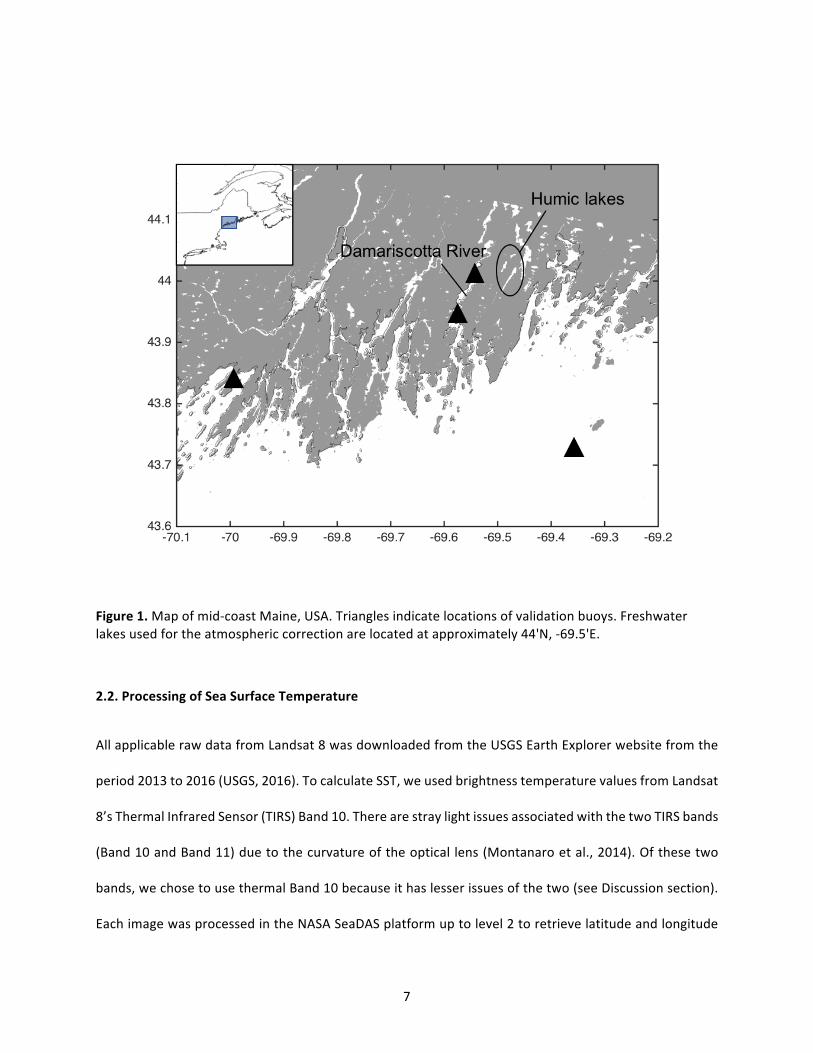
2.1.StudyArea

ThecoastofMaine includesa seriesof fjards (shallowerandbroader fjords)and jaggedembayments

carved by receding glaciers during the Pleistocene epoch. In situ samples were collected and ocean

monitoring buoy systems were maintained in two of these estuaries, the Damariscotta River and

HarpswellSound,overthecourseofseveralyearsandweusedthemheretovalidateLandsat-8derived

productsontheMainecoast(trianglesonFigure1).WechosetofocusontheDamariscottaRiverbecause

ithasexistingaquacultureoperations (currently75%of theoystersproduced inMaine, (MaineDMR,

2015))andsuitablesamplingaccess.TheDamariscottaRiverEstuaryis29kilometerslong,hasamean

summerflushingtimeof4to5weeks,andisdominatedbystrongtideswithamplitudesofupto3.35m

(McAlice,1977).Sedimentresuspensioninthisestuaryishighestatlowtide,andlowestathightide.The

estuary is highly saline, ranging from 25 to 32.5 psu,with a small amount of freshwater input from

DamariscottaLakeintoSaltBayatitsnorthernreach.Thesubstrateisasoft,muddybottomcomposed

ofclaytosandysiltswithanaveragedepthof15.25m.TheseattributesmaketheDamariscottaRiveran

idealplaceforgrowingmarket-sizeoystersandotherbivalvespecies,andmakeitanexcellentreference

pointforexpandingtheaquacultureindustryalongthecoastofMaine.

7

Figure1.Mapofmid-coastMaine,USA.Trianglesindicatelocationsofvalidationbuoys.Freshwaterlakesusedfortheatmosphericcorrectionarelocatedatapproximately44'N,-69.5'E.

2.2.ProcessingofSeaSurfaceTemperature

AllapplicablerawdatafromLandsat8wasdownloadedfromtheUSGSEarthExplorerwebsitefromthe

period2013to2016(USGS,2016).TocalculateSST,weusedbrightnesstemperaturevaluesfromLandsat

8’sThermalInfraredSensor(TIRS)Band10.TherearestraylightissuesassociatedwiththetwoTIRSbands

(Band10andBand11)duetothecurvatureoftheoptical lens(Montanaroetal.,2014).Ofthesetwo

bands,wechosetousethermalBand10becauseithaslesserissuesofthetwo(seeDiscussionsection).

EachimagewasprocessedintheNASASeaDASplatformuptolevel2toretrievelatitudeandlongitude

8

arrays,ageo-registeredimage,andtheassociatedland/cloudmask(georeferencingismaintained,asitis

providedfromUSGS).

RegressionsbetweencoincidentatmosphericallycorrectedAVHRRsatellitederivedSSTandthat

derivedfromLandsat8’sbrightnesstemperaturewereusedtocreateanSSTproductfortheLandsat8

imagery (similar to Thomas et al., 2002). This regression process, de-facto, acts as the atmospheric

correction for theLandsatSSTproduct1)assuming that theatmospheredoesnotchange in the time

intervalbetweenAVHRRandLandsatoverlappingimageand2)theatmosphereishomogenousacross

theLandsatscene.ExampledatafromthisprocedurearedisplayedonFigure2below.Ofthefourtoeight

AVHRRimagescapturedonthesamedayasLandsat8,wesubjectivelychosetheimagewiththeleast

amountofcloudcoverandpoorlymaskedpixels,bestgeolocation,andcleanestSSTpatterns, for the

regression(seeAppendixAfordetaileddescription).Thedatafortheregressionwasselectedfromcloud

free and offshore areas to accommodate the lower AVHRR resolution (1 km versus Landsat 8 100m

resolution).ThebestresultswereachievedusingcloudfreeareaswithahighdynamicrangeinSST.The

resultingregressionequationbetweenthesignalofLandsat’sBand10andtheAVHRR-basedtemperature

wasthenappliedtoprovideSSTforthefullresolutionLandsat8image.

Ingeneral,thereareapproximatelyfourAVHRRimagesperday.Duetochangingcloudcoverand

orbitconfigurationbetweenavailableAVHRRimages,itwassometimesnecessarytouseanimagemore

distantintime(butlesscloudy)fromtheLandsat8overpass,despiteatemporallymoreproximateone

beingavailable.However,becauseGulfofMaineSSTpatternschangeslowly(lessthan0.4oCover12hours

atbuoy44005,www.neracoos.org),weconsiderthisanacceptabletradeofftomaximizethenumberof

qualityAVHRRpixelsthatwillbeusedintheregression.ThemeanoffsettimebetweentheLandsat8and

AVHRRoverpasseswas6.8hours,withaminimumoffsetof2.3hours,maximumoffsetof30.2hours,and

astandarddeviationof5.8hours.TheentireareaofoverlapbetweenAVHRRoceanpixelsandLandsat8

9

oceanpixelsisusedformostscenes.Landsat8imagesweresubsampledtoevery10thpixelinbothxand

ydimensionstoreducethedatavolumefortheregressions,andAVHRRimageswereresampledtomatch

the30m(interpolatedfrom100m)resolutionoftheLandsatB10usingnearestneighborresamplingin

MATLAB.Dependingonthedistributionofclouds, theregressionareawasrestrictedtoareaswithout

cloudcontamination(orpoorlymaskedclouds)insomeinstances.Cloudandlandweredilatedbytwo

pixels in the AVHRR image to reduce occurrences of cloud ringing artifacts and nearshore land

contamination.Theregressionprocesswas iterative.Aftereach iteration,allLandsat8andcoincident

AVHRRpixelsthatweregreaterthanonestandarddeviationfromthelinearbestfitlineoftherelationship

wereremovedandtheregressionwasre-calculatedwiththeremainingdata.Theiterationprocesswas

repeateduntil thePearsoncorrelationcoefficient for the twodatasetsstabilizedorstarted toworsen

(whichisduetouncertaintiesintheapproach).Thefinalregressionequationwasthenappliedtoeach

Landsat8B10pixelatthefull30mresolutiontoobtainaLandsatSSTimage.

2.3.OceanColor

Oceancolormultispectraldata,whichrespondstotheeffectsofoceanicparticlesanddissolved

matter,aremeasuredfromspacebytheOperationalLandImager(OLI)radiometeronboardLandsat8.

Theradiancemeasuredincludescontributionsfromthetarget(thesurfacewatercolumn),theairwater

interface,andthebackground(particlesandgasesfromnearbypixelsandparticlesintheatmosphere)

(Mobleyetal.,2016).Toobtaininformationontheoceanicconstituents,theatmosphericcontributionto

the signal needs to be removed (a process known as ‘atmospheric correction’ see below). From the

correctedwater-leavingradiance,wecomputedthereflectance(denotedasR,-)fromwhichtheproducts

ofturbidityandChlaarederived.

10

2.4.AtmosphericCorrectionfor𝐑𝐫𝐬

Giventhelowturbidityinourareaofinvestigation(seeSection2.5below),wechosetouseacombination

oftheNearInfrared(NIR)andShortWaveInfrared(SWIR)channelsforatmosphericcorrectioninSeaDAS.

TheNIRwasimportanttousebecauseof itshighersignal/noiseratio(NIRbandshadratiosof6and7

whileSWIRbandshadratiosof9and10)inlowturbiditywaters,andtheSWIRwasimportantbecauseit

hasthestrongestabsorptionforwaterwhichhelpsdifferentiatein-watersedimentsfromatmospheric

aerosolparticles(Franzetal.,2015;Pahlevanetal.,2014).Applyingthisatmosphericcorrectionovera

sceneresultedinaper-pixelcorrection,eachwithitsownangstromcoefficient.Theangstromcoefficient

istheslopeofthespectralaerosolopticalthickness,whichisderivedrelativetoareferencewavelength

(usually443nm/865nmasoutputfromSeaDAS).Weadjustedthiscoefficientbecausetheautomaticper-

pixelretrievalsprovidedbySeaDASresultedinnegativevaluesinseveralfreshwaterareasthatwereblack

bodytargetsforouratmosphericcorrectionschemeandshouldhavenear-zeroorpositiveretrievals.The

primary reason for adjusting the angstrom is that the aerosolmodels used for processing data from

satellitessuchasSeaWiFsandMODIS(Ahmadetal.,2010),donotrepresenttheaerosolconditionsfor

ourstudyarea,thecoastofMaine(Pahlevanetal.,2017).Wethenchoseasingleangstromcoefficient

perscene(fromwithinthedistributionofinvertedangstromvalues),byrequiringthattheminimalvalue

ofR,-(443)inascene,measuredinaveryhumiclake,benearzero.Mostfreshwaterlakesonthecoast

ofMainearehumicandhavehighlevelsofchromophoricdissolvedorganicmatter,CDOM,whichgives

themabrownhueandattenuateslightquickly(RoeslerandCulbertson,2016;Rasmussen,1989).Several

freshwaterlakeswithhighCDOMwithinourstudyregion(MuddyPond,BiscayPond,andDamariscotta

PondcircledinFig.1)wereselectedassuitablereferencetargetstocorrecttheentireLandsat8scene.In

each individualsatellite image,thedarkest lake(whereR,-(443) isnearzero)wasusedtodetermine

angstrom coefficient. Analysis of a sample of water from one of these lakes verified that the

expectedR,-(443) is zero within the uncertainty of the measurement (Appendix Table B1). We

11

subsequentlyappliedtheretrievedangstrominSeaDAStotheentirescenetorecalculateR,-atevery

wavelength.R,-valueswerethenusedtocomputeturbidityandchlorophyll.

2.5.RetrievalofTurbidity

Turbidity,T,(notethat1gL-1ofSPMisequivalent,withintherangeofvaluesfoundinourstudyarea,to

aturbidityof1NTU(PfannkucheandSchmidt,2003))wascalculatedovertheentiresatellitesceneusing

atmosphericallycorrected𝑅"#(655)andthefollowingequationfromNechadetal.(2010):

𝑇 = 𝐴;𝜌'

1 − 𝜌'/𝐶;[𝑔𝑚DE](1)

where 𝜌' = 𝑅"#(655) ∗ 𝜋 and 𝜌'is the atmospherically corrected and derived water leaving

reflectance,𝐴;=289.1and𝐶;=16.86(Nechadetal.,2010).

2.6.RetrievalofChlorophyll-𝐚

Chl𝑎wascalculatedusingthestandardOC3algorithm(O’Reillyetal.,1998)fromtheNASAOceanBiology

ProcessingGroup,usingtheabove-calculated𝑅"#:

logLM 𝑐ℎ𝑙𝑜𝑟_𝑎 = 𝑎M + 𝑎U logLM𝑅"# 𝜆%WXY𝑅"# 𝜆*"YYZ

U[

U\L

(2)

whereaManda_aresensorspecificcoefficients,andR,- λabcd andR,- λe,ddf arethegreatestofvalues

from443>483and555nm,respectively,ontheOLIsensoraboardLandsat8(NASA,2016).(Note:SeaDAS

applies coefficients to convertbroadband Landsat8-basedR,- to11nmnarrowbands forwhich this

equationwasdeveloped).

12

2.7.Validationwithinsitudata

Validationwascarriedoutforphysicalandbiogeochemicalparameters(SST,turbidity,andChl𝑎)using

data from water samples and three oceanographic buoy observing systems. Historical data was

downloaded from the NERACOOS (Northeastern Regional Association of Coastal Ocean Observing

Systems) buoys E01 and I01 operated by the University of Maine, Orono, in the Gulf of Maine, a

Land/OceanBiogeochemicalObservatory(LOBO)buoyatBowdoinCollegeinHarpswellSound,andtwo

LOBO buoys at the University of Maine’s Darling Marine Center in the Damariscotta River (Fig. 1,

NERACOOSBuoyI01notpictured).TheLOBObuoyswereequippedwithsensorsthatremainatadepth

of1.5metersandmaintainedandcleanedtopreventbiofoulingeverytwoweeks.Temperaturedatawere

collectedfromallthreeobservingsystemsandcomparedtoLandsat8SST.Atotalof52matchupswere

identifiedoriginatingfrom31clearoverpassesfrom2013to2016.

Insituturbiditywasusedtovalidatesatellite-derivedturbidityduringeightoverpassesin2015

and 2016. Data were collected from the UMaine LOBO buoys in the Damariscotta River, and were

measuredbyaWETLabsWQMsensorcapableofmeasuringturbidityfrom0–25NTU(thatmeasurelight

scattered in the back direction at a 20 nm bandwidth around 700 nm). This sensor was vicariously

calibratedagainstaHachturbiditysensor(whichisanISO7027:1999turbiditystandard).Thebuoydata

werecorrectedbyaregressionbetweenHachturbiditysamplesandtheLOBOturbiditywithaslopefactor

of1.58(AppendixTableB2).

InsituChl𝑎wasusedtovalidatesatellite-derivedChl𝑎duringthesameeightoverpassesin2015

and2016.InsituChl𝑎dataweremeasuredbytheDamariscottaRiverLOBObuoys’WETLabsfluorescent

sensorcapableofmeasuringChl𝑎concentrationsfrom0–50µgL-1.Thebuoydatawascorrectedbya

regressionbetweenextractedChl𝑎samplesandtheLOBOChlawithaslopefactorof1.71.Watersamples

werecollectedintriplicate,atthesurface,andinopaquebottleswithin30minutesofeachoverpassand

13

filteredforextractiononaTurner10AUfluorometerperstandardprotocol(Holm-HansonandRiemann,

1978).

2.8.SatelliteImageryforanOysterSuitabilityIndex

AnOysterGrowthSuitabilityIndexwasdesignedusingthesatellite-derivedSST,turbidity,andChl𝑎.A

weightingandindexingprocedureofthesethreephysicalparametersdescribedideal,moderate,andpoor

conditions forgrowingmarket sizedoysters in surfaceculture.Thecriteria for the indexwerechosen

basedonpublishedstudiesofenvironmentaleffectsonoystergrowth,recognizingthattheconcentration

oforganicdetritus,knowntobeanimportantcomponentofoysterdiet,wasnotavailable.Temperature

isthemost importantvariable inoystergrowth,especially inthecoldwatersofcoastalMainesince it

controlsthefiltrationrateofoysters(andthereforegivenanimportanceweightfactorof80%;Loosanoff,

1958;Hoffmannetal.,1992;EhrichandHarris,2015).Oysterclearanceofalgaeisapositivefunctionof

algaeconcentration,aslargeamountsofpseudofecesareproducedathighalgalconcentrations.Because

ofthis,weweightedChlaat15%,withpoorconditionsbeinglessthan1μgL-1orgreaterthan10μgL-1,

moderateconditionsbeing1to3μgL-1,andidealconditionsasto10μgL-1(EpifanioandEwart,1977;

Hawkinsetal.,2013).Turbidity,asestimatedbysuspendedparticulatematter,hasanegativeeffecton

oyster feeding at high concentrations, by diluting algal cellswith largely inorganicmatter.Haven and

Morales-Alamo (1966) observed large amounts of pseudofeces production by Eastern oysters at

concentrationsofsuspendedparticulatematterabove10mgL-1,thuswegaveturbidityaweightof5%

anddesignatedpoorconditionsasgreaterthan10μgL-1,moderateconditionsbetween8and10μgL-1

and idealconditionsunder8μgL-1. Hoffmanetal. (1992)alsomodeledoyster filtrationasapositive

functionofwatertemperatureandanegativefunctionofhighsuspendedloads.

Theserelativeweightswerechosenasastartingpointfortheindexandcouldberefinedinfuture

iterations to optimize the index (Gong et al., 2012), by doing a sensitivity analysis of the relative

14

importance of the factors concomitant with growth measurements and growth model outputs. The

resultingOysterSuitabilityIndexisthesumoftheweightedconditionsonascalefrom0to1,wherepixels

withavalueof1representwaterswhereanoysterislikelytogrowtomarketsizewithin2years:

𝑂𝑆𝐼 = 𝑆𝐼U×𝑤U

Z

U\L

(3)

where𝑆𝐼U isthevalueoftheenvironmentalvariablei,𝑤Uistheweightofthevariablei,andnisthenumber

ofenvironmental variables.Wecombined images fromeachyearduring the samemonth to createa

monthlyaveragedindex.Note:thisindexdoesnotincludeinformationaboutsiteclosures,bottomdepth,

orresidentialrestrictions.Futureworkshouldincludethisinformationforamorecomprehensiveindex.

15

CHAPTER3

RESULTS

3.1.Satelliteretrievedvalidationwithinsitudata

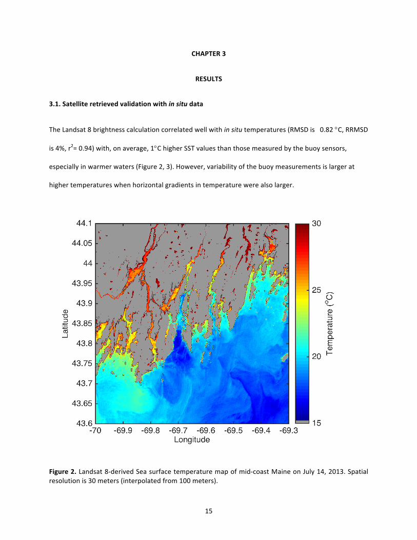
TheLandsat8brightnesscalculationcorrelatedwellwithinsitutemperatures(RMSDis0.82°C,RRMSD

is4%,r2=0.94)with,onaverage,1°ChigherSSTvaluesthanthosemeasuredbythebuoysensors,

especiallyinwarmerwaters(Figure2,3).However,variabilityofthebuoymeasurementsislargerat

highertemperatureswhenhorizontalgradientsintemperaturewerealsolarger.

Figure2.Landsat8-derivedSeasurfacetemperaturemapofmid-coastMaineonJuly14,2013.Spatialresolutionis30meters(interpolatedfrom100meters).

16

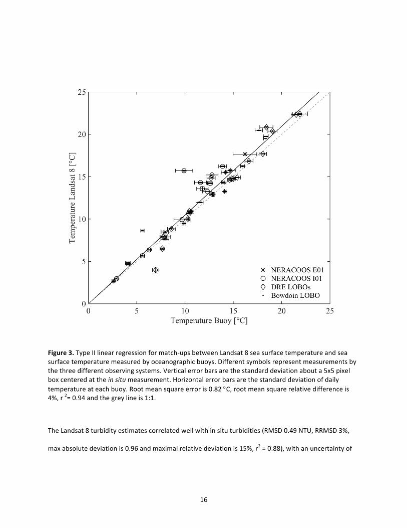
Figure3.TypeIIlinearregressionformatch-upsbetweenLandsat8seasurfacetemperatureandseasurfacetemperaturemeasuredbyoceanographicbuoys.Differentsymbolsrepresentmeasurementsbythethreedifferentobservingsystems.Verticalerrorbarsarethestandarddeviationabouta5x5pixelboxcenteredattheinsitumeasurement.Horizontalerrorbarsarethestandarddeviationofdailytemperatureateachbuoy.Rootmeansquareerroris0.82°C,rootmeansquarerelativedifferenceis4%,r2=0.94andthegreylineis1:1.

TheLandsat8turbidityestimatescorrelatedwellwithinsituturbidities(RMSD0.49NTU,RRMSD3%,

maxabsolutedeviationis0.96andmaximalrelativedeviationis15%,r2=0.88),withanuncertaintyof

17

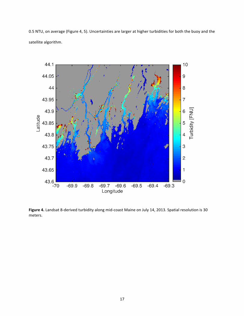
0.5NTU,onaverage(Figure4,5).Uncertaintiesarelargerathigherturbiditiesforboththebuoyandthe

satellitealgorithm.

Figure4.Landsat8-derivedturbidityalongmid-coastMaineonJuly14,2013.Spatialresolutionis30meters.

18

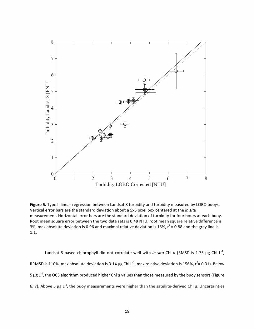
Figure5.TypeIIlinearregressionbetweenLandsat8turbidityandturbiditymeasuredbyLOBObuoys.Verticalerrorbarsarethestandarddeviationabouta5x5pixelboxcenteredattheinsitumeasurement.Horizontalerrorbarsarethestandarddeviationofturbidityforfourhoursateachbuoy.Rootmeansquareerrorbetweenthetwodatasetsis0.49NTU,rootmeansquarerelativedifferenceis3%,maxabsolutedeviationis0.96andmaximalrelativedeviationis15%,r2=0.88andthegreylineis1:1.

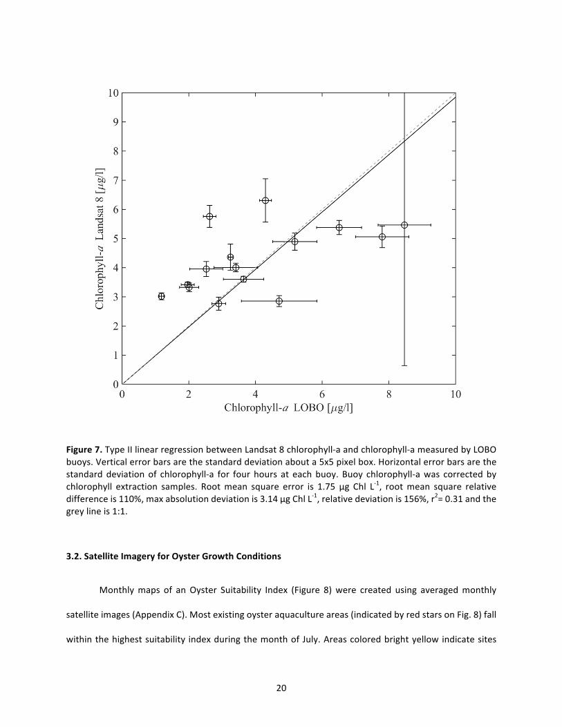
Landsat-8based chlorophyll didnot correlatewellwith in situ Chla (RMSD is 1.75μgChl L-1,

RRMSDis110%,maxabsolutedeviationis3.14μgChlL-1,maxrelativedeviationis156%,r2=0.31).Below

5μgL-1,theOC3algorithmproducedhigherChl𝑎valuesthanthosemeasuredbythebuoysensors(Figure

6,7).Above5μgL-1,thebuoymeasurementswerehigherthanthesatellite-derivedChl𝑎.Uncertainties

19

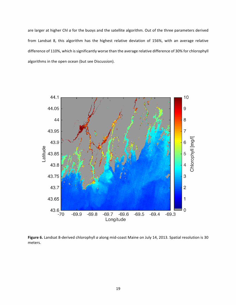
arelargerathigherChlaforthebuoysandthesatellitealgorithm.Outofthethreeparametersderived

from Landsat 8, this algorithm has the highest relative deviation of 156%, with an average relative

differenceof110%,whichissignificantlyworsethantheaveragerelativedifferenceof30%forchlorophyll

algorithmsintheopenocean(butseeDiscussion).

Figure6.Landsat8-derivedchlorophyllaalongmid-coastMaineonJuly14,2013.Spatialresolutionis30meters.

20

Figure7.TypeIIlinearregressionbetweenLandsat8chlorophyll-aandchlorophyll-ameasuredbyLOBObuoys.Verticalerrorbarsarethestandarddeviationabouta5x5pixelbox.Horizontalerrorbarsarethestandarddeviationof chlorophyll-a for four hours at eachbuoy. Buoy chlorophyll-awas correctedbychlorophyll extraction samples. Rootmean square error is 1.75 μg Chl L-1, rootmean square relativedifferenceis110%,maxabsolutiondeviationis3.14μgChlL-1,relativedeviationis156%,r2=0.31andthegreylineis1:1.

3.2.SatelliteImageryforOysterGrowthConditions

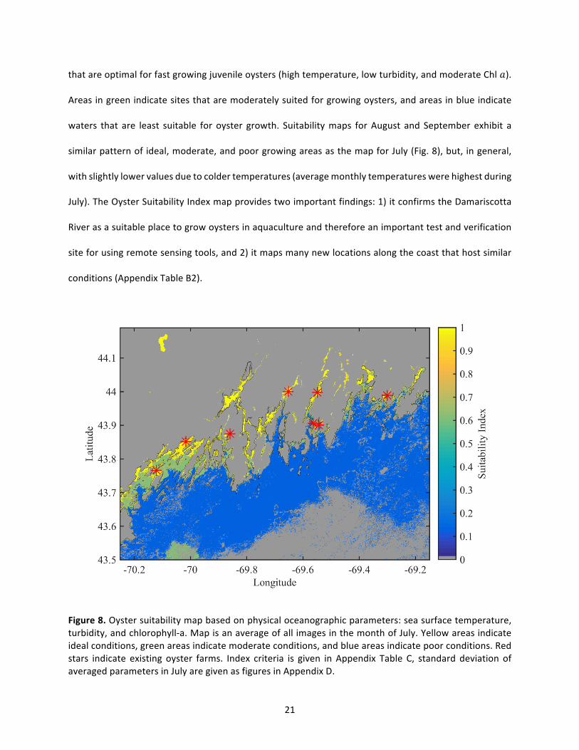
Monthlymaps of anOyster Suitability Index (Figure 8)were created using averagedmonthly

satelliteimages(AppendixC).Mostexistingoysteraquacultureareas(indicatedbyredstarsonFig.8)fall

withinthehighestsuitability indexduringthemonthofJuly.Areascoloredbrightyellowindicatesites

21

thatareoptimalforfastgrowingjuvenileoysters(hightemperature,lowturbidity,andmoderateChl𝑎).

Areasingreenindicatesitesthataremoderatelysuitedforgrowingoysters,andareasinblueindicate

waters that are least suitable for oyster growth. Suitabilitymaps forAugust and September exhibit a

similarpatternofideal,moderate,andpoorgrowingareasasthemapforJuly(Fig.8),but, ingeneral,

withslightlylowervaluesduetocoldertemperatures(averagemonthlytemperatureswerehighestduring

July).TheOysterSuitabilityIndexmapprovidestwoimportantfindings:1)itconfirmstheDamariscotta

Riverasasuitableplacetogrowoystersinaquacultureandthereforeanimportanttestandverification

siteforusingremotesensingtools,and2)itmapsmanynewlocationsalongthecoastthathostsimilar

conditions(AppendixTableB2).

Figure8.Oystersuitabilitymapbasedonphysicaloceanographicparameters:seasurfacetemperature,turbidity,andchlorophyll-a.MapisanaverageofallimagesinthemonthofJuly.Yellowareasindicateidealconditions,greenareasindicatemoderateconditions,andblueareasindicatepoorconditions.Redstars indicate existing oyster farms. Index criteria is given in Appendix Table C, standard deviation ofaveragedparametersinJulyaregivenasfiguresinAppendixD.

22

CHAPTER4

DISCUSSION

4.1.SatelliteImagery

The correspondence between the Landsat 8 satellite derived products and in situ measurements

demonstratesthecapabilityofgeneratingSST,turbidity,andChlamapsalongthejaggedcoastofMaine.

Whilethesedatashowencouragingresults,thereareseveralfactorsfromourstudythatcouldimprove

thepresentalgorithms.Straylightissuesariseifthetemperaturefromanobjectoutsideofthefieldof

viewof the imageraffectsapixelwithin the fieldofview.Fortunately,mostwateralong thecoastof

Maineisvigorouslytidallymixed(~3mtidalrange),andthusdatafromthecenterofchannelscanbe

usedtoinfertheSSTconcentrationsthroughoutthosechannels(ThorntonandMayer,2015).Withinthe

estuaries, however, a TIRS pixel (which is three times as wide as an OLI pixel) next to landmay be

incorrectlycolder(ifthelandiscolder)orwarmer(ifthelandiswarmer).However,thematch-upswith

temperature and turbidity products suggest adjacency and stray light have not degraded the data

significantly,anddifferencesarelikelyduetonoiseasopposedtosystematicbias.

4.2.LimitationsinValidationProcess

Validationof Landsat8 imagerywith in situmeasurements isnecessary toassess theaccuracyof the

algorithms for retrieving bio-physical products. Someof thediscrepancy between in situ and satellite

matchupscanbeexplained,whileothers require further investigation.Onereason thatLandsat8SST

valuesmaybehigherthanmostbuoymeasurements(Fig.3)isbecausetheSSTestimatescomefromlight

emitted from the top fewmicrometers of the sea surface,while the buoy sensors are located about

1.5mbelowthesurface.Inthedaytimeimages,thesubsurfacewaterislikelycoolerthanthesurface

skindue tophysicalandenvironmental factors (Padulaetal.,2010;Donlonetal.,2002;Ward,2006).

23

Despitethisbias,theLandsat8SST(derivedbyregressingwithAVHRR)performedwellalongthecoastof

Maine(Fig.3)andourresultssuggestthatourapproachcouldbeusedasatoolformeasuringSSTwhere

highspatialresolutionisdesired.

Avigoroussemi-diurnaltidecharacterizestheDamariscottaRiveranddeliversshelfwater into

theupperreachesoftheestuary.Thetidalcyclewasevidentinthedailyturbiditysignal(notshown)from

the LOBObuoys: at low tide, there are elevated levels of turbiditywhereas at high tide there is less

turbidity(duetotheincreaseinturbidityfromthemouthtotheendoftheestuary).Thehorizontalerror

barsinFigure5representthevariabilityduringafour-hourperiodaroundeachsatelliteoverpasstime,

and highlight the importance of simultaneous sampling for in situ - satellitematchups. The turbidity

algorithmperformswellwithinouruncertaintiesinthiscontext.

Landsat 8 Chl a often differs significantly from the LOBO buoy measurements. There are

significantuncertaintiesassociatedwithbothmeasurementtechniques(Cullen,2008).Landsat8Chlais

retrievedfromR,-usinganalgorithmcalibratedintheopenocean,whereastheLOBObuoysmeasure

Chlafluorescencewhichisregressedagainstwatersamples.EstimatingChlafromfluorescenceisthe

mostcommonwaytomeasureChlabutisaffectedbyseveralprocessesthatcontributetouncertainty.

Theseincludechangesinfluorescenceyieldduetovariabilityinthealgaltaxonomy,nutrientstress,and

photo-acclimation,tonameafew(Cullen,1982).Inaddition,concentrationsofphytoplanktonhavebeen

observedintheDamariscottaRivertovaryontimescalesofhours(ThompsonandPerry,2006).

Non-photochemical quenching (NPQ; when phytoplankton decrease their fluorescence at a

maximumlightharvestinglevel,e.g.Cullen,1982)contributestovariability.However,wefindnighttime

measurements to be comparable to daytimemeasurements (Appendix Fig. B.1) for theDamariscotta

River.Therefore,theoffsetinChlaislikelynotduetoerrorsinducedbyNPQ.Anotherpotentialerroris

associatedwiththeOC3algorithm,whichestimatesChlaasaratioof𝑅"#intheblueandgreenchannels.

24

The blue channel is especially affected by colored dissolved organic material (CDOM). Independent

changesofCDOMwillaffecttheOC3chlorophyllestimate(Siegeletal.,2005).AlongthecoastofMaine,

where there are coastal forests andmarshes, CDOM is in high concentration and variable (Roesler&

Culbertson,2016). Incoastalareasandestuaries rich inCDOMit is likely thatabsorptionbydissolved

organicmatterwouldbias theOC3algorithm. It is likely thata localalgorithm that takes localCDOM

concentrationintoaccount,couldimproveChlaretrievalsfromLandsat8.

4.3.OysterSuitabilityIndex

TheOysterSuitabilityIndexprovidedinthispaperisintendedasasupplementtoothertoolsthat

determineoptimaloystergrowingareas.Firstly,thesatelliteimagesprovideonlyaclimatologicalmonthly

snapshotofcoastaltemperatureproducts,whichprovideslesstemporalresolutionthanacomprehensive

daydegreemodelfortemperature-dependentshellfishgrowth.Secondly,moreimportantenvironmental

factorssuchassalinity,waterdepth,bottomtypeandwatervelocity(necessaryforoystergrowing),are

not considered.Organicdetritus is known tobean important componentofbivalvediets (Dameand

Patten,1981;Bayneetal.,1993;Barilleetal.,1997),butcurrentlycannotbemeasuredusingsatellite

imagery.Ourindexthereforeprovidesguidanceonsuitablewaterqualityconducivetorapidgrowth,but

notsufficientinformationtomodelsitespecificproductioncapacityforsuspendedorbottomculture.

Althoughsatellitethermaldataisonlysensitivetothetemperatureofthetopfewmicrometers

ofwater,andoceancolorissensitiveonlytooneopticaldepth(whichvaries,butontheMainecoastis

usuallythetoponeortwometers),thesedataarerelevanttothewholewatercolumnifthewatercolumn

is often vertically well-mixed. Indeed, many estuaries on the Maine coast are well-mixed (e.g. the

SheepscotandMedomakRivers,ThorntonandMayer,2015;Mayer,1996),whichcoincidentlyqualifyfor

oysteraquacultureinoursuitabilityindex(AppendixTableB2).Finally,localknowledgeisinvaluablefor

25

the expansion of an existing industry on the coast of Maine, and stakeholder input is essential for

improvingsuchanindexwithlocalinformationsuchassiteaccessibility,townordinances,etc.

4.4.FutureWork

Continuedsamplingduringthespringandsummerof2017willprovideamorecompletedataset

foroptimizingoceancolorproducts inMaine.A localalgorithmforLandsat8Chlaalongthecoastof

Mainecouldbeconstructedwithadditional insitusamplescollectedduringsatelliteoverpasses.There

areseveralapproachestotunealocalalgorithm.Anempiricalapproach,suchastheOC3algorithm,uses

arelationshipbetweeninsitumeasurementsandratiosofthesatellitesensorbands.Asecondmethod

involvesusingageneralizedinherentopticalpropertiesinversion(GIOP,Werdelletal.,2013).Thismethod

solvesforChla,SPM,andCDOMusingknownspectralshapesofopticalproperties(forphytoplankton

and non-algal absorption and backscattering by particles) and known values of absorbance and

backscatteringofwater(whichareweakfunctionsofsalinityandtemperature).Databasesofcollection

sites locatedintheDamariscottaRiverandHarpswellSoundcouldtunetheshapesofinherentoptical

propertiesfortheGIOPalgorithmandprovideanestimateofChlainthesetwoestuaries.Furthermore,

insitusamplesfromvariouslocationsalongthecoastwillvalidatethelocalalgorithmsothatitsusecan

beexpandedfromtheDamariscottaRivertootherplacesalongthecoast.

ObtainingmoreparametersfromLandsat8,suchascoloreddissolvedorganicmatter(CDOM),

wouldprovideadditional information to growers aswell as environmentalmonitoringandecosystem

managers.Franzetal.,(2015)andSloneckeretal.,(2015)describethepotentialofusingLandsat8for

remotesensingofCDOMinconjunctionwithinsitumeasurements.AreliableCDOMproductwouldalso

improvethealgorithmforChla,asthepresenceofCDOMoftencontributestoanoverestimationofChl

a.Furthermore,highlevelsofCDOMarecorrelatedwithlowsalinityincertainestuariesinMaine(Carder

etal.,1989;D’Saetal.,2002;Mayer,L.,2017personalcommunication).Itwouldbehelpfultoidentify

26

areas with significant freshwater influx because these often bring concentrations of bacteria that

negativelyaffectclammingandotherfisheries(Kleindinstetal.,2014;Shumwayetal.,1988).

27

CHAPTER5

CONCLUSION

OursatellitedataderivedOysterSuitabilityIndexcanactasapowerfultoolforoysteraquaculture

site selection and the expansion of the shellfish farming industry. It shows that suitable biophysical

conditionsforoystergrowthexistinmanyareasoftheMainecoast.Suitabilityindicesforotherbivalve

species,suchasmussels,scallops,andfinfishalongthecoast,orotherapplicationsrequiringhighspatial

resolution,canbedevelopedbasedonthealgorithmspresentedhere.SST,turbidity,andChlaretrieved

fromLandsat8issufficientlyvalidatedbyinsitumatchups(within+/-1°CforSST;maxabsolutedeviation

is0.96NTUand relativedeviation is15% for turbidity;andmaxabsolutedeviation is3μgChl L-1and

relativedeviationis156%forChla).OurresultsshowthatLandsat8imageryisusefulforretrievingSST,

turbidity,andChlaincoastalwatersofMaine,USA,andcanbeappliedtoothernarrowestuariesaround

theworld.ThenoveltyofusingLandsat8inthiscontextoffersauniqueopportunitytomapandmonitor

coastal waters at an unprecedented spatial resolution. Inclusion of data from other satellites with

complimentarysensorsuitessuchasSentinel2A,andtherecentlylaunchedSentinel2B,couldimprove

boththespatialandtemporalcoverageofcoastalwaters,astheywillprovidefive-dayorbettercoverage

(unfortunately,Sentinel2AandBdonothavethermalbands).SSTdatafromLandsat8isespeciallyuseful

for aquaculture site prospecting. We recommend adding thermal bands to future high resolution

missions,asmorefrequentSSTdatawillassistbothsiteselectionforaquacultureandotherapplications.

Futureworkimprovingbiogeochemicallocalalgorithms,refiningtheatmosphericcorrection,andadding

other parameters such as CDOM,will further advance the use of high resolution remote-sensing for

coastalapplications.

28

REFERENCES

Ahmad,Z.,Franz,B.a,McClain,C.R.,Kwiatkowska,E.J.,Werdell,J.,Shettle,E.P.,&Holben,B.N.(2010).Newaerosolmodelsfortheretrievalofaerosolopticalthicknessandnormalizedwater-leavingradiancesfromtheSeaWiFSandMODISsensorsovercoastalregionsandopenoceans.AppliedOptics,49(29),5545.

AguilarManjarrez,J.&Crespi,V.(2013).FAOAquacultureNewsletter55,September2016.

Barillé,L.,Prou,J.,Héral,M.andRazet,D.,(1997).Effectsofhighnaturalsestonconcentrationsonthefeeding,selection,andabsorptionoftheoysterCrassostreagigas(Thunberg).Journalofexperimentalmarinebiologyandecology,212(2),pp.149-172.

Barnes,R.A.,Holmes,A.W.,&Esaias,W.E.(1995).StrayLightintheSeaWiFSRadiometer.SeaWiFSTechnicalReportSeries,31(July),79.

Barnes,T.K.,Volety,A.K.,Chartier,K.,Mazzotti,F.J.andPearlstine,L.,(2007).Ahabitatsuitabilityindexmodel for theeasternoyster (Crassostreavirginica), a tool for restorationof theCaloosahatcheeEstuary,Florida.JournalofShellfishResearch,26(4),pp.949-959.

Bayne,B.L.,Iglesias,J.I.P.,Hawkins,A.J.S.,Navarro,E.,Heral,M.andDeslous-Paoli,J.M.,(1993).Feedingbehaviourofthemussel,Mytilusedulis:responsestovariationsinquantityandorganiccontentoftheseston.JournaloftheMarineBiologicalAssociationoftheUnitedKingdom,73(04),pp.813-829.

Buitrago,J.,Rada,M.,Hernández,H.andBuitrago,E.,(2005).Asingle-usesiteselectiontechnique,usingGIS,foraquacultureplanning:choosinglocationsformangroveoysterraftcultureinMargaritaIsland,Venezuela.EnvironmentalManagement,35(5),pp.544- 556.

CakeJr.,E.W.,(1983).Habitatsuitabilityindexmodels:GulfofMexicoAmericanoyster(No.82/10.57).U.S.FishandWildlifeService.

Carrasco,M.F.andBarón,P.J., (2010).Analysisof thepotentialgeographic rangeof thePacificoysterCrassostrea gigas (Thunberg, 1793) based on surface seawater temperature satellite data andclimatecharts:thecoastofSouthAmericaasastudycase.BiologicalInvasions,12(8),pp.2597-2607.

Carder,K.L.,Steward,R.G.,Harvey,G.R.,&Ortner,P.B.(1989).Marinehumicandfulvicacids:Theireffectsonremotesensingofoceanchlorophyll.LimnologyandOceanography,34(l),68–81.http://doi.org/10.4319/lo.1989.34.1.0068

Congleton,W.R.,Pearce,B.R.,Parker,M.R.andBeal,B.F.,(1999).Mariculturesiting:aGISdescriptionofintertidalareas.EcologicalModelling,116(1),pp.63-75.

Cullen,J.J.(1982).Thedeepchlorophyllmaximum:Comparingverticalprofilesofchlorophylla.CanadianJournalofFisheriesandAquaticSciences,39(5),791-803.doi:10.1139/f82-108.

29

Cullen,J.J.,(2008).Observationandpredictionofharmfulalgalblooms.InM.Babin,C.S.RoeslerandJ.J.Cullen[eds.],Real-timecoastalobservingsystemsforecosystemdynamicsandharmfulalgalblooms,UNESCO.

Dame,R.F.andPatten,B.C.,(1981).Analysisofenergyflowsinanintertidaloysterreef.Mar.Ecol.Prog.Ser,5(2),pp.115-124.

D'Sa,E.,Hu,C.,Muller-Karger,F.,&Carder,K.(2002).Estimationofcoloreddissolvedorganicmatterandsalinityfieldsincase2watersusingSeaWiFS:Examplesfrom FloridaBayandFloridaShelf.JournalofEarthSystemScience,111(3)197-207.

Dogliotti,A.I.,Ruddick,K.G.,Nechad,B.,Doxaran,D.,&Knaeps,E.(2015).Asinglealgorithmtoretrieveturbidityfromremotely-senseddatainallcoastalandestuarinewaters.RemoteSensingofEnvironment,156,157–168.http://doi.org/10.1016/j.rse.2014.09.020

Donlon,C.J.,Minnett,P.J.,Gentemann,C.,Nightingale,T.J.,Barton,I.J.,Ward,B.,&Murray,M.J.(2002).Towardimprovedvalidationofsatelliteseasurfaceskintemperaturemeasurementsforclimateresearch.JournalofClimate,15(4),353–369.http://doi.org/10.1175/1520-0442(2002)015<0353:TIVOSS>2.0.CO;2

Ehrich,M.K.,&Harris,L.A.(2015).Areviewofexistingeasternoysterfiltrationratemodels.EcologicalModelling,297,201–212.http://doi.org/10.1016/j.ecolmodel.2014.11.023

Epifanio,C.E.andEwart,J.,1977.MaximumrationoffouralgaldietsfortheoysterCrassostreavirginicaGmelin.Aquaculture,11(1),pp.13-29.

Estapa,M.L.,Boss,E.,Mayer,L.M.,&Roesler,C.S.(2012).Roleofironandorganiccarboninmass-specificlightabsorptionbyparticulatematterfromLouisianacoastalwaters.LimnologyandOceanography,57(1),97–112.http://doi.org/10.4319/lo.2012.57.1.0097

Franz,B.a.,Bailey,S.W.,Kuring,N.,&Werdell,P.J.(2015).OceancolormeasurementswiththeOperationalLandImageronLandsat-8:implementationandevaluationinSeaDAS.JournalofAppliedRemoteSensing,9(1),96070.http://doi.org/10.1117/1.JRS.9.096070

Gong,C.,Chen,X.,Gao,F.,&Chen,Y.(2012).Importanceofweightingformulti-variablehabitatsuitabilityindexmodel:Acasestudyofwinter-springcohortofOmmastrephesbartramiiintheNorthwesternPacificOcean.JournalofOceanUniversityofChina,11(2),241–248.http://doi.org/10.1007/s11802-012-1898-6

Haven,D.S.andMorales-Alamo,R.,1966.Aspectsofbiodepositionbyoystersandotherinvertebratefilterfeeders.Limnol.Oceanogr,11(4),pp.487-498.

Hawkins,a.J.S.,Pascoe,P.L.,Parry,H.,Brinsley,M.,Cacciatore,F.,Black,K.D.,…Zhu,M.Y.(2013).ComparativeFeedingonChlorophyll-RichVersusRemainingOrganicMatterinBivalveShellfish.JournalofShellfishResearch,32(3),883–897.http://doi.org/10.2983/035.032.0332

30

Hawkins,A.J.S.,Pascoe,P.L.,Parry,H.,Brinsley,M.,Black,K.D.,McGonigle,C.,Moore,H.,Newell,C.R.,O'Boyle,N.,Ocarroll,T.andO'Loan,B.,(2013).Shellsim:agenericmodelofgrowthandenvironmentaleffectsvalidatedacrosscontrastinghabitatsinbivalveshellfish.JournalofShellfishResearch,32(2),pp.237-253

Hoffmann,E.E.,Powell,E.N.,Klinck,J.M.andWilson,E.A.(1992).ModelingoysterpopulationsIII.Criticalfeedingperiods,growth.JournalofShellfishResearch,11(2),pp.399-416.

Holm-Hansen,O.,andB.Riemann.(1978).Chlorophylladetermination:improvementsinmethodology.Oikos,30:438-447.

Hudson,A.S.,Talke,S.A.,&Jay,D.A.(2016).UsingSatelliteObservationstoCharacterizetheResponseofEstuarineTurbidityMaximatoExternalForcing.EstuariesandCoasts,1–16.http://doi.org/10.1007/s12237-016-0164-3

Kleindinst,J.L.,Anderson,D.M.,McGillicuddy,D.J.,Stumpf,R.P.,Fisher,K.M.,Couture,D.A.,…Nash,C.(2014).CategorizingtheseverityofparalyticshellfishpoisoningoutbreaksintheGulfofMaineforforecastingandmanagement.Deep-SeaResearchPartII:TopicalStudiesinOceanography,103,277–287.http://doi.org/10.1016/j.dsr2.2013.03.027

Gernez,P.,Lerouxel,A.,Mazeran,C.,Lucas,A.,&Barill,L.(2014).Remotesensingofsuspendedparticulatematterinturbidoyster-farmingecosystems.JournalofGeophysicalResearch:Oceans,7277–7294.http://doi.org/10.1002/2014JC010055.

Loosanoff, V.L., (1958). Someaspectsof behavior of oysters at different temperatures.TheBiologicalBulletin,114(1),pp.57-70.

Mayer,L.M.,UniversityofMaineatOrono.,&UniversityofMaine/UniversityofNewHampshireSeaGrantCollegeProgram.(1996).TheKennebec,SheepscotandDamariscottaRiverEstuaries:Seasonaloceanographicdata.Orono,Me:Dept.ofOceanography,UniversityofMaine.

McAlice,B.J.(1977).ApreliminaryoceanographicsurveyofDamariscottaRiverEstuary,LincolnCounty,Maine.Washington:U.S.NationalOceanicandAtmosphericAdministration.

Mobley,C.D.,Werdell,J.,Franz,B.,Ahmad,Z.,&Bailey,S.(2016).AtmosphericCorrectionforSatelliteOceanColorRadiometryATutorialandDocumentationNASAOceanBiologyProcessingGroup.

Montanaro,M.,Gerace,A.,Lunsford,A.,&Reuter,D.(2014).Straylightartifactsinimageryfromthelandsat8thermalinfraredsensor.RemoteSensing,6(11),10435–10456.http://doi.org/10.3390/rs61110435

NASA.(2016).https://oceancolor.gsfc.nasa.gov/atbd/chlor_a/

Nechad,B.,Ruddick,K.G.,&Park,Y.(2010).Calibrationandvalidationofagenericmultisensoralgorithmformappingoftotalsuspendedmatterinturbidwaters.RemoteSensingofEnvironment,114(4),854–866.http://doi.org/10.1016/j.rse.2009.11.022

31

Newell,R.I.E.andJordan,S.J.,(1983).PreferentialingestionoforganicmaterialbytheAmericanoysterCrassostreavirginica.Marineecologyprogressseries.Oldendorf,13(1),pp.47-53.

Newell,C.R.,S.Shumway,T.L.CucciandR.Selvin.(1989).Theeffectsofnaturalsestonparticlesizeand typeon feeding rates, feeding selectivity and food resource availability for themusselMytilusedulisLinnaeus,1758atbottomculturesitesinMaine.J.Shellfish.Res.8:187-196.

Newell, C.R., A.J.S. Hawkins, K. Morris, J. Richardson, C. Davis and T. Getchis. (2013).ShellGIS:adynamictoolforshellfishfarmsiteselection.WorldAquaculture.44:50-53.

O’Reilly, J.E.,Maritorena,S.,Mitchell,B.G.,Siegel,D.A.,Carder,K.L.,Garver,S.A.,…McClain,C.R.(1998).Oceancolor chlorophyll algorithm forSeaWiFS. JournalofGeophysicalResearch,103(Cll),24937–24953.

Pahlevan,N.,Lee,Z.,Wei,J.,Schaaf,C.B.,Schott,J.R.,&Berk,A.(2014).On-orbitradiometriccharacterizationofOLI(Landsat-8)forapplicationsinaquaticremotesensing.RemoteSensingofEnvironment,154,272–284.http://doi.org/10.1016/j.rse.2014.08.001

Pahlevan,N.,Sarkar,S.,&Franz,B.A.(2016).Uncertaintiesincoastaloceancolorproducts:Impactsofspatialsampling.RemoteSensingofEnvironment,181,14–26.http://doi.org/10.1016/j.rse.2016.03.022

Pahlevan,N.,Sheldon,P.,Peri,F.,Wei,J.,Shang,Z.,Sun,Q.,…Loveland,T.(2016).Calibration/validationoflandsat-derivedoceancolourproductsinBostonharbour.InternationalArchivesofthePhotogrammetry,RemoteSensingandSpatialInformationSciences-ISPRSArchives,41(July),1165–1168.http://doi.org/10.5194/isprsarchives-XLI-B8-1165-2016

Pérez,O.M.,Ross,L.G.,Telfer,T.C.anddelCampoBarquin,L.M.,(2003).WaterqualityrequirementsformarinefishcagesiteselectioninTenerife(CanaryIslands):predictivemodellingandanalysisusingGIS.Aquaculture,224(1),pp.51-68.

Pérez-Camacho,A.,Aguiar,E.,Labarta,U.,Vinseiro,V.,Fernández-Reiriz,M.J.andÁlvarez-Salgado,X.A.,(2014).Ecosystem-basedindicatorsasatoolformusselculturemanagementstrategies.EcologicalIndicators,45,pp.538-548.

Pfannkuche,J.,&Schmidt,A.(2003).Determinationofsuspendedparticulatematterconcentrationfromturbiditymeasurements: Particle size effects and calibration procedures.Hydrological Processes,17(10),1951–1963.http://doi.org/10.1002/hyp.1220

Powell,E.N.,Hofmann,E.E.,Klinck,J.M.andRay,S.M.,(1992).Modelingoysterpopulations1.Acommentaryonfiltrationrate.Isfasteralwaysbetter?J.ShellfishRes.,1I:387-398.

Radiarta,I.N.,Saitoh,S.I.,&Miyazono,A.(2008).GIS-basedmulti-criteriaevaluationmodelsforidentifyingsuitablesitesforJapanesescallop(Mizuhopectenyessoensis)aquacultureinFunkaBay,southwesternHokkaido,Japan.Aquaculture,284(1–4),127–135.

32

Rasmussen,J.B.,Godbout,L.,&Schallenburg,M.(1989).Thehumiccontentoflakewateranditsrelationshiptowatershedandlakemorphometry.LimnologyandOceanography,34(7),1336-1343.

Rheault,R.B.,&Rice,M.A.(1996).Food-limitedgrowthandconditionindexintheeasternoyster,Crassostreavirginica(Gmelin1791),andthebayscallop,Argopectenirradiansirradians(Lamarck1819).JournalofShellfishResearch,15(2),

Roesler,C.,&Culbertson,C.(2016).LakeTransparency :AWindowintoDecadalVariationsinDissolvedOrganicCarbonConcentrationsinLakesofAcadiaNational.http://doi.org/10.1007/978-3-319-30259-1

Shumway,S.E.,Sherman-Caswell,S.,&Hurst,J.(1988).ParalyticshellfishpoisoninginMaine:monitoringamonster.JournalofShellfishResearch.

Siegel,D.A.,Maritorena,S.,Nelson,N.B.,&Behrenfeld,M.J.(2005).Independenceandinterdependenciesamongglobaloceancolorproperties:Reassessingthebio-opticalassumption.JournalofGeophysicalResearchC:Oceans,110(7),1–14.http://doi.org/10.1029/2004JC002527

Slonecker,E.T.,Jones,D.K.,&Pellerin,B.A.(2015).ThenewLandsat8potentialforremotesensingofcoloreddissolvedorganicmatter(CDOM).MarinePollutionBulletin,107(2),518–527.http://doi.org/10.1016/j.marpolbul.2016.02.076

Soniat,T.M.andBrody,M.S.,(1988).FieldvalidationofahabitatsuitabilityindexmodelfortheAmericanoyster.EstuariesandCoasts,11(2),pp.87-95.

Thomas, A., Byrne, D., andWeatherbee, R. (2002). Coastal sea surface temperature variability fromLandsatinfrareddata.RemoteSens.Environ.81,262–272.

Thomas,Y.,Mazurié,J.,Alunno-Bruscia,M.,Bacher,C.,Bouget,J.F.,Gohin,F.,…Struski,C.(2011).Modellingspatio-temporalvariabilityofMytilusedulis(L.)growthbyforcingadynamicenergybudgetmodelwithsatellite-derivedenvironmentaldata.JournalofSeaResearch,66(4),308–317.http://doi.org/10.1016/j.seares.2011.04.015

Thompson,B.P.,&Perry,M.J.(2006).TemporalandSpatialVariabilityofPhytoplanktonBiomassintheDamariscottaRiverEstuary,Maine,USA.DepartmentofMarineSciences,Masterof.

Thornton,K.,&Mayer,L.(2015).MaineCoastalObservingAlliance,SummaryReport2014.

Tissot,C.,Brosset,D.,Barillé,L.,LeGrel,L.,Tillier,I.,Rouan,M.andLeTixerant,M.,(2012).Modelingoysterfarmingactivitiesincoastalareas:agenericframeworkandpreliminaryapplicationtoacasestudy.CoastalManagement,40(5),pp.484-500.

USGS.(2016).L8OLI/TIRSproduct.https://earthexplorer.usgs.gov

Vanhellemont,Q.,&Ruddick,K.(2014).TurbidwakesassociatedwithoffshorewindturbinesobservedwithLandsat8.RemoteSensingofEnvironment,145,105–115.

33

Wang,H.,Hladik,C.M.,Huang,W.,Milla,K.,Edmiston,L.,Schalles,J.F.,…Edmiston,L.(2010).Detectingthespatialandtemporalvariabilityofchlorophyll-aconcentrationandtotalsuspendedsolidsinApalachicolaBay,FloridausingMODISimagery.InternationalJournalofRemoteSensing,1161(December2016).http://doi.org/10.1080/01431160902893485

Wang,P.,Boss,E.S.,&Roesler,C.(2005).Uncertaintiesofinherentopticalpropertiesobtainedfromsemianalyticalinversionsofoceancolor.AppliedOptics,44(19),4074–4085.http://doi.org/10.1364/AO.44.004074

Ward,B.(2006).Near-surfaceoceantemperature.JournalofGeophysicalResearch:Oceans,111(2),1–18.http://doi.org/10.1029/2004JC002689

Widdows,J.,Fieth,P.andWorrall,C.M.,(1979).Relationshipsbetweenseston,availablefoodandfeedingactivityinthecommonmusselMytilusedulis.MarineBiology,50(3),pp.195-207.

34

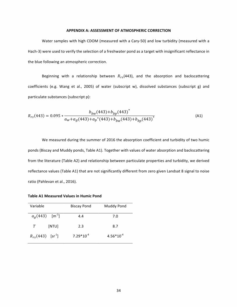
APPENDIXA:ASSESSMENTOFATMOSPHERICCORRECTION

WatersampleswithhighCDOM(measuredwithaCary-50)andlowturbidity(measuredwitha

Hach-3)wereusedtoverifytheselectionofafreshwaterpondasatargetwithinsignificantreflectancein

thebluefollowinganatmosphericcorrection.

Beginning with a relationship between 𝑅"#(443), and the absorption and backscattering

coefficients (e.g. Wang et al., 2005) of water (subscript w), dissolved substances (subscript g) and

particulatesubstances(subscriptp):

𝑅"# 443 = 0.095 ∗𝑏𝑏𝑤(443)+𝑏𝑏𝑝(443)

∗

𝑎𝑤+𝑎𝑔(443)+𝑎𝑝∗(443)+𝑏𝑏𝑤(443)+𝑏𝑏𝑝(443)∗ (A1)

Wemeasuredduringthesummerof2016theabsorptioncoefficientandturbidityoftwohumic

ponds(BiscayandMuddyponds,TableA1).Togetherwithvaluesofwaterabsorptionandbackscattering

fromtheliterature(TableA2)andrelationshipbetweenparticulatepropertiesandturbidity,wederived

reflectancevalues(TableA1)thatarenotsignificantlydifferentfromzerogivenLandsat8signaltonoise

ratio(Pahlevanetal.,2016).

TableA1MeasuredValuesinHumicPond

Variable BiscayPond MuddyPond

𝑎* 443 [m-1] 4.4 7.0

𝑇[NTU] 2.3 8.7

𝑅"# 443 [sr-1] 7.29*10-4 4.56*10-4

35

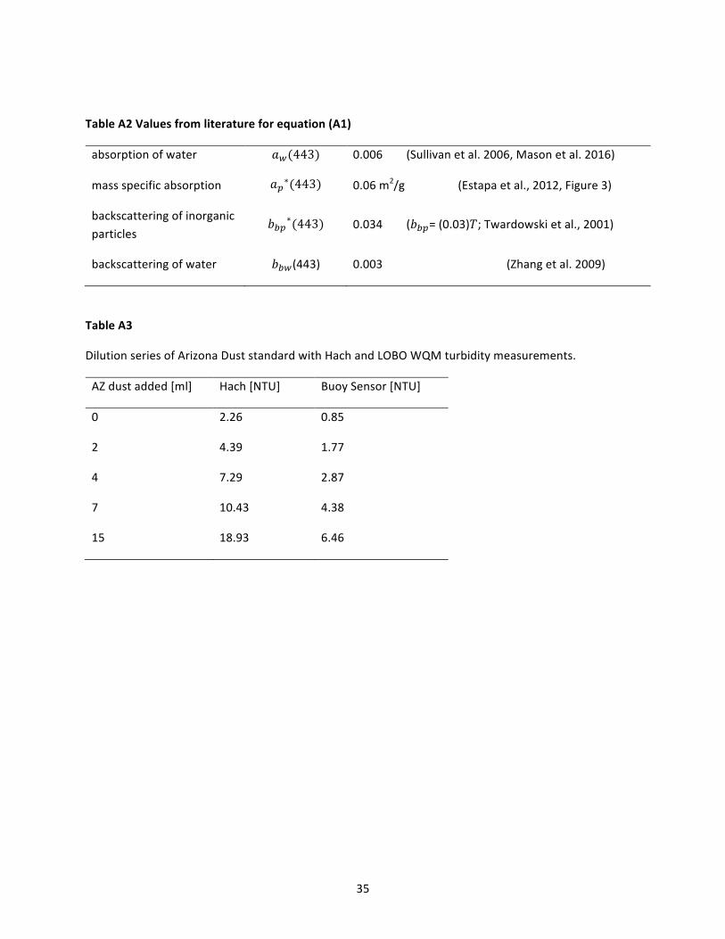
TableA2Valuesfromliteratureforequation(A1)

absorptionofwater 𝑎'(443) 0.006(Sullivanetal.2006,Masonetal.2016)

massspecificabsorption 𝑎&∗(443) 0.06m2/g(Estapaetal.,2012,Figure3)

backscatteringofinorganicparticles

𝑏%&∗(443) 0.034(𝑏%&=(0.03)𝑇;Twardowskietal.,2001)

backscatteringofwater 𝑏%'(443) 0.003(Zhangetal.2009)

TableA3

DilutionseriesofArizonaDuststandardwithHachandLOBOWQMturbiditymeasurements.

AZdustadded[ml] Hach[NTU] BuoySensor[NTU]

0 2.26 0.85

2 4.39 1.77

4 7.29 2.87

7 10.43 4.38

15 18.93 6.46

36

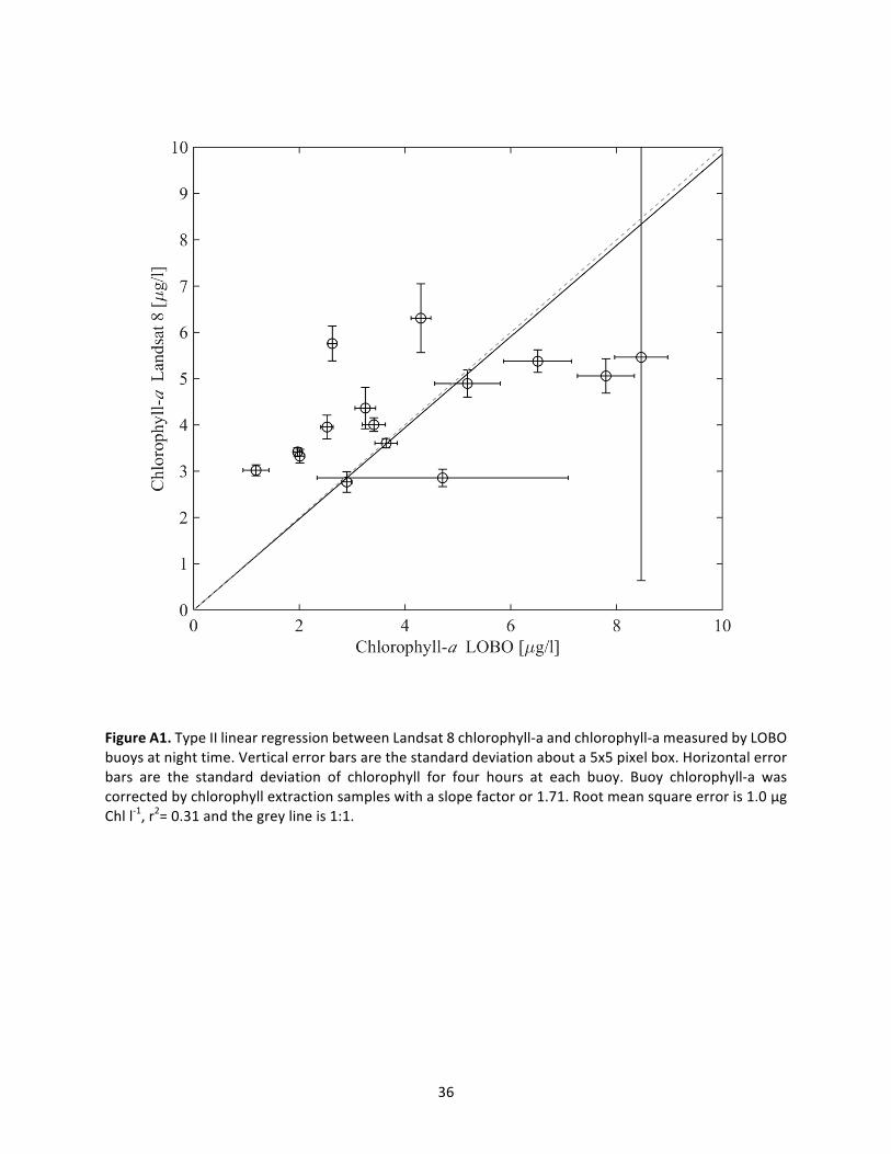
FigureA1.TypeIIlinearregressionbetweenLandsat8chlorophyll-aandchlorophyll-ameasuredbyLOBObuoysatnighttime.Verticalerrorbarsarethestandarddeviationabouta5x5pixelbox.Horizontalerrorbars are the standard deviation of chlorophyll for four hours at each buoy. Buoy chlorophyll-a wascorrectedbychlorophyllextractionsampleswithaslopefactoror1.71.Rootmeansquareerroris1.0μgChll-1,r2=0.31andthegreylineis1:1.

37

APPENDIXB.OYSTERSUITABILITYINDEX

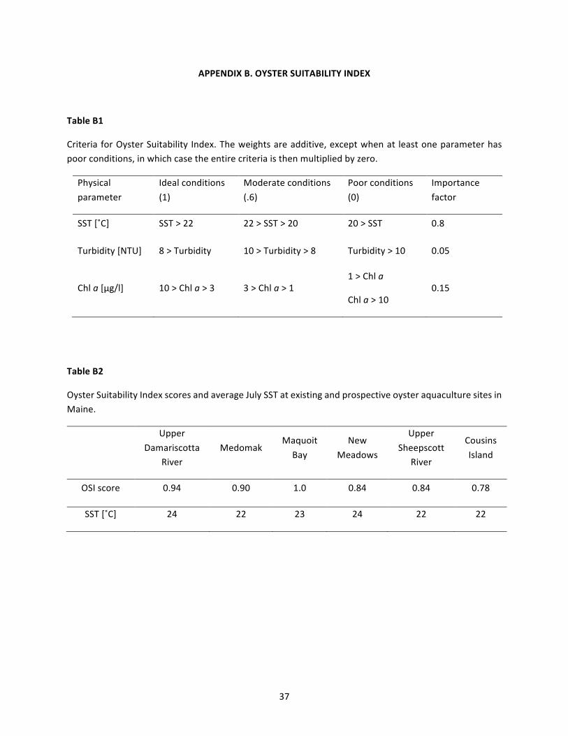
TableB1

CriteriaforOysterSuitability Index.Theweightsareadditive,exceptwhenat leastoneparameterhaspoorconditions,inwhichcasetheentirecriteriaisthenmultipliedbyzero.

Physicalparameter

Idealconditions(1)

Moderateconditions(.6)

Poorconditions(0)

Importancefactor

SST[˚C] SST>22 22>SST>20 20>SST 0.8

Turbidity[NTU] 8>Turbidity 10>Turbidity>8 Turbidity>10 0.05

Chla[μg/l] 10>Chla>3 3>Chla>11>Chla

Chla>100.15

TableB2

OysterSuitabilityIndexscoresandaverageJulySSTatexistingandprospectiveoysteraquaculturesitesinMaine.

Upper

DamariscottaRiver

MedomakMaquoit

BayNew

Meadows

UpperSheepscott

River

CousinsIsland

OSIscore 0.94 0.90 1.0 0.84 0.84 0.78

SST[˚C] 24 22 23 24 22 22

38

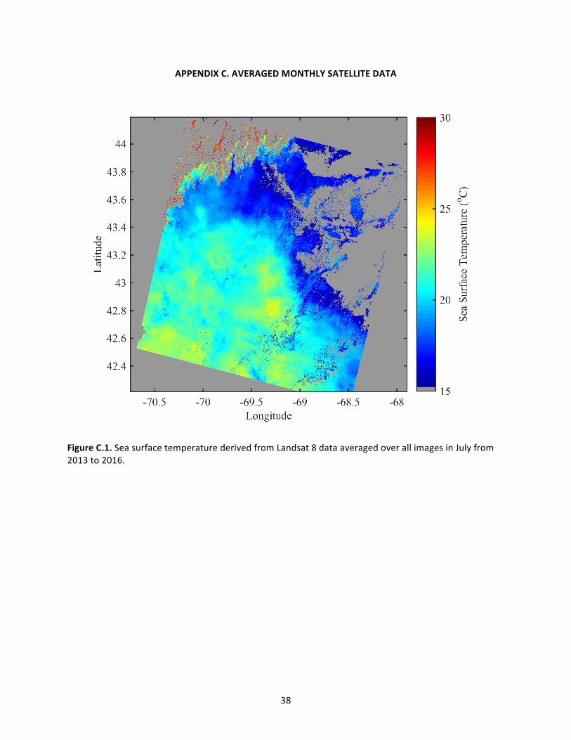
APPENDIXC.AVERAGEDMONTHLYSATELLITEDATA

FigureC.1.SeasurfacetemperaturederivedfromLandsat8dataaveragedoverallimagesinJulyfrom2013to2016.

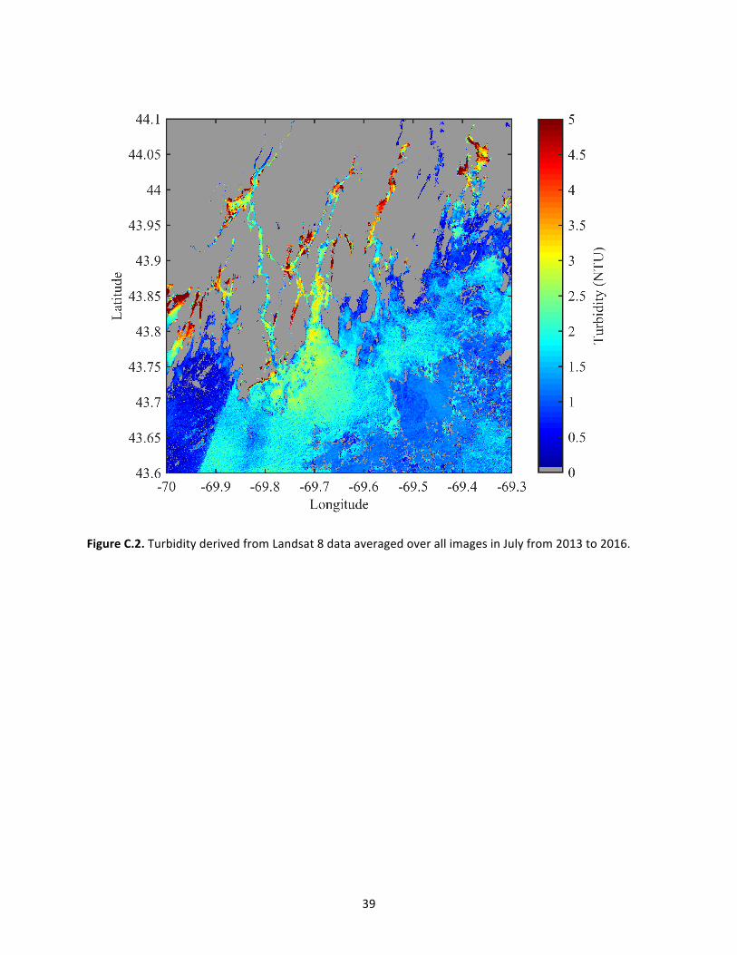
39

FigureC.2.TurbidityderivedfromLandsat8dataaveragedoverallimagesinJulyfrom2013to2016.

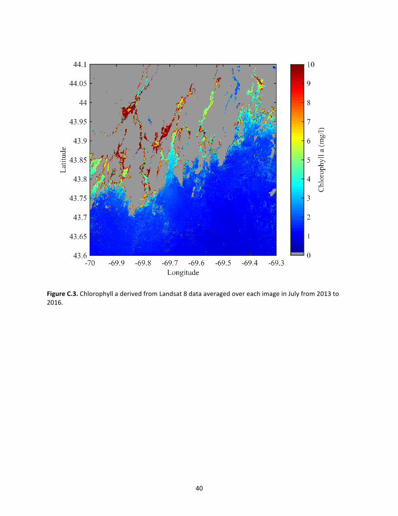
40

FigureC.3.ChlorophylladerivedfromLandsat8dataaveragedovereachimageinJulyfrom2013to2016.

41

APPENDIXD.STANDARDDEVIATIONOFMONTHLYCLIMATOLOGYMAPS

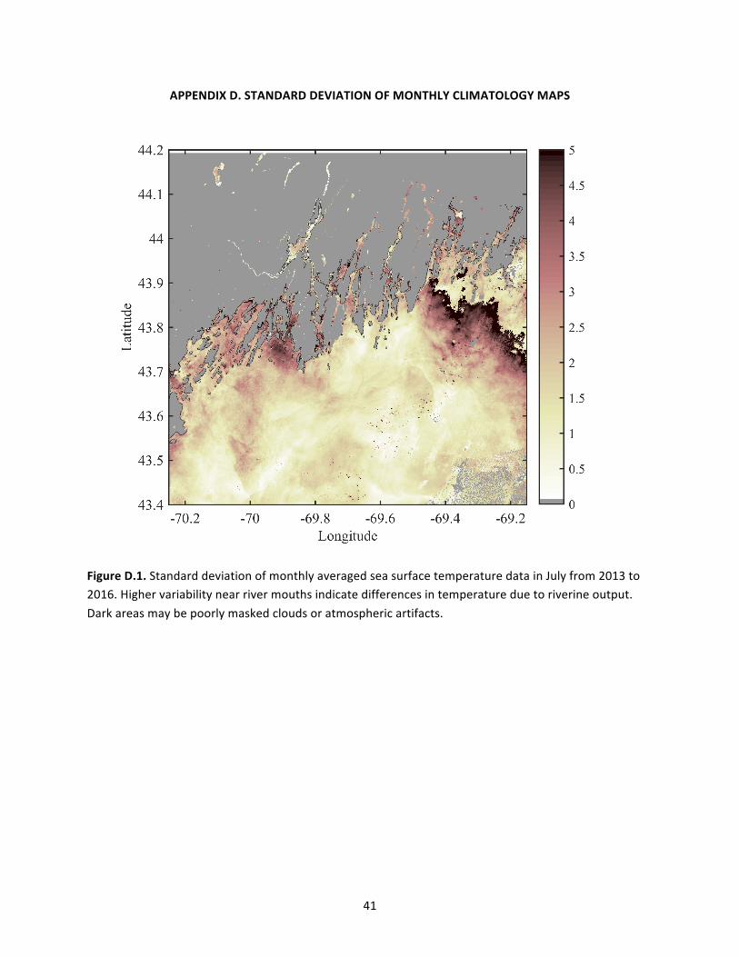
FigureD.1.StandarddeviationofmonthlyaveragedseasurfacetemperaturedatainJulyfrom2013to2016.Highervariabilitynearrivermouthsindicatedifferencesintemperatureduetoriverineoutput.Darkareasmaybepoorlymaskedcloudsoratmosphericartifacts.

42

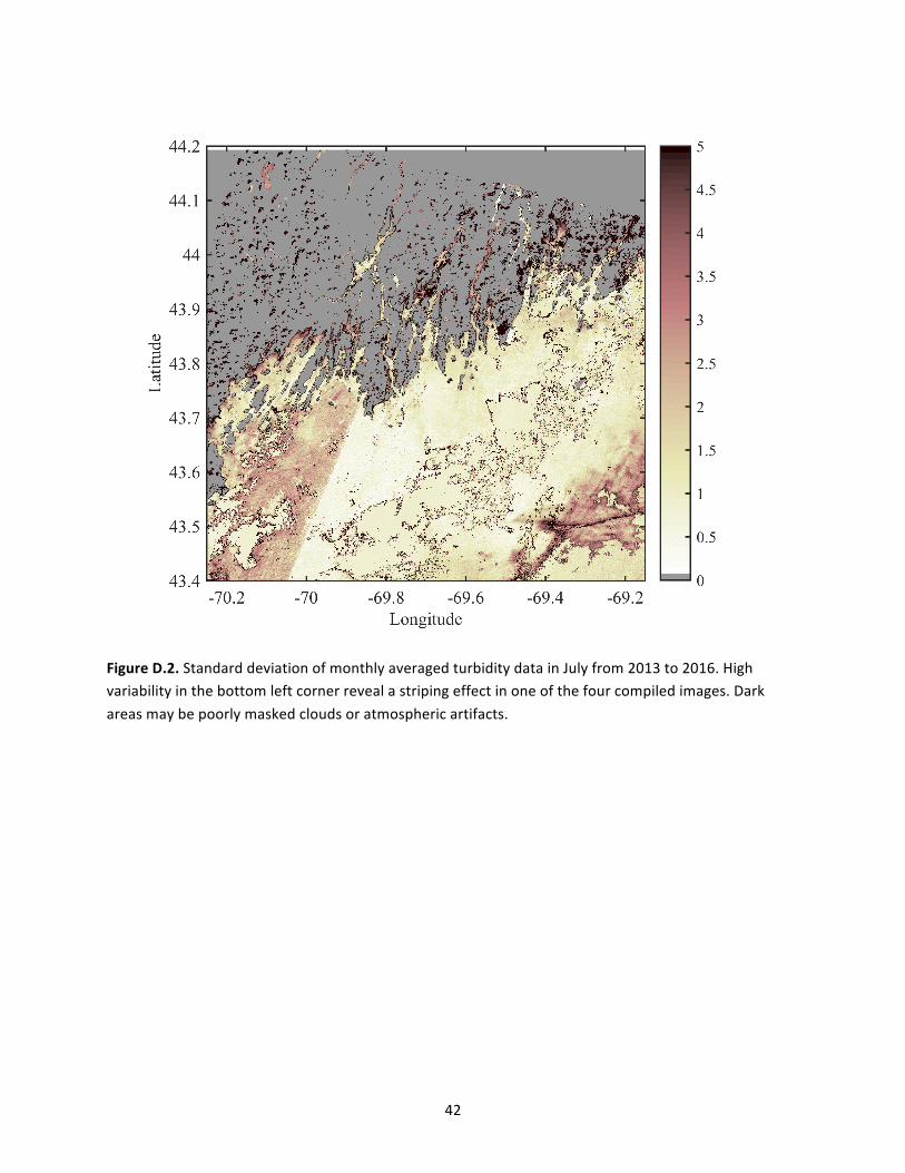
FigureD.2.StandarddeviationofmonthlyaveragedturbiditydatainJulyfrom2013to2016.Highvariabilityinthebottomleftcornerrevealastripingeffectinoneofthefourcompiledimages.Darkareasmaybepoorlymaskedcloudsoratmosphericartifacts.

43

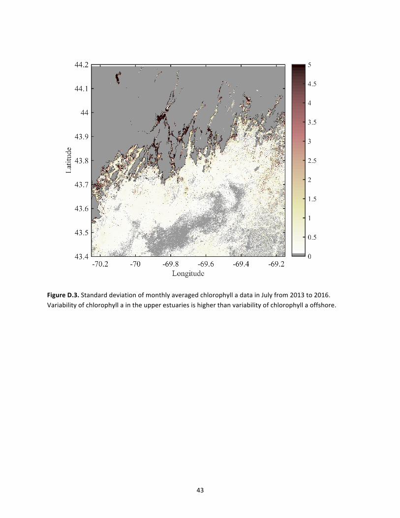
FigureD.3.StandarddeviationofmonthlyaveragedchlorophylladatainJulyfrom2013to2016.Variabilityofchlorophyllaintheupperestuariesishigherthanvariabilityofchlorophyllaoffshore.

44

BIOGRAPHYOFTHEAUTHOR

JordanSnyderwasborninAnaheim,CaliforniaonDecember13,1990.Shewasraisedin

HuntingtonBeach,CaliforniaandgraduatedfromHuntingtonBeachHighSchoolin2009.Sheattended

theUniversityofCalifornia,Davisandgraduatedin2013withaBachelor’sdegreeinGeology.She

movedtoMaineandenteredtheOceanographygraduateprogramatTheUniversityofMaineinthe

summerof2015.Sheenjoyssurfing,SCUBAdiving,running,hiking,camping,gardening,cookingand

laughing.JordanisacandidatefortheMasterofSciencedegreeinOceanographyfromtheUniversityof

MaineinAugust2017.