Factorization algebras and free field theories

Owen Gwilliam

Contents

Acknowledgements vii

Chapter 1. Introduction 11.1. An overview of the chapters 31.2. Notations 4

Chapter 2. Motivation and algebraic techniques 72.1. Classical BV formalism: the derived critical locus 82.2. Quantum BV formalism: the twisted de Rham complex 102.3. Wick’s lemma and Feynman diagrams, homologically 172.4. A compendium of essential definitions and constructions 242.5. The homological perturbation lemma in the BV formalism 272.6. Global observables and formal Hodge theory 34

Chapter 3. BV formalism as a determinant functor 393.1. Cotangent quantization of k-vector spaces 413.2. Recollections 443.3. Properties of cotangent quantization over any commutative dg algebra 483.4. Invertibility survives over artinian dg algebras 51

Chapter 4. Factorization algebras 594.1. Definitions 604.2. Associative algebras as factorization algebras on R 634.3. Associative algebras and the bar complex 664.4. The category of factorization algebras 734.5. General construction methods for factorization algebras 754.6. A novel construction of the universal enveloping algebra 784.7. Extension from a factorizing basis 814.8. Pushforward and Pullback 83

Chapter 5. Free fields and their observables 875.1. Introduction 875.2. Elliptic complexes and free BV theories 905.3. Observables as a factorization algebra 945.4. BV quantization as a Heisenberg Lie algebra construction 985.5. BV quantization as a determinant functor 100

iii

5.6. Implications for interacting theories 1015.7. Theories with a Poincare lemma 102

Chapter 6. Free holomorphic field theories and vertex algebras 1056.1. The βγ system 1066.2. The quantum observables of the βγ system 1086.3. Recovering a vertex algebra 1226.4. Vertex algebras from Lie algebras 1276.5. Definitions and a conjecture 133

Chapter 7. An index theorem 1377.1. A motivating example 1397.2. A precise statement of the theorem 1407.3. Setting up the problem 1447.4. Background about BV theories and renormalization 1487.5. The proof 1557.6. Global statements 159

Bibliography 163

iv

ABSTRACT. We study the Batalin-Vilkovisky (BV) formalism for quantization of field theories in sev-eral contexts. First, we extract the essential homological procedure and study it from the perspectiveof derived algebraic geometry. Our main result here is that the BV formalism provides a naturaldeterminant functor we call “cotangent quantization,” sending a perfect R-module to an invertibleR-module and quasi-isomorphisms to quasi-isomorphisms, where R is an artinian commutative dif-ferential graded algebra over a field of characteristic zero. Second, we introduce the formalism offactorization algebras, a local-to-global object much like a sheaf, and describe several perspectiveson how the BV formalism makes the observables of a free quantum field theory into a factorizationalgebra. We study in detail the free βγ system, a holomorphic field theory living on any Riemann sur-face, and we recover the βγ vertex algebra from the factorization algebra of quantum observables. Wealso construct the factorization algebras on a Riemann surface that recover the vertex algebras arisingfrom affine Kac-Moody Lie algebras. Finally, we study quantization of families of elliptic complexes.Our main result here is an index theorem relating the associated family of factorization algebras tothe determinant line of the family of elliptic complexes. At the heart of our work is the formalism forperturbative quantum field theory developed by Costello [Cos11] and for the associated observablesby Costello-Gwilliam [CG], and this thesis provides an exposition of the ideas and techniques in anaccessible context.

v

Acknowledgements

This thesis appears thanks to the support and encouragement of many people.

Through all my endeavors, mathematical and otherwise, I am sustained by the love and trustof my family. The Gwilliams of Evanston have made this town home for me and hosted gracefullysome of the most important events of my life. With profound warmth, the Hermanns have wel-comed me into their midst and made me a part of their family. My sister Natalie offers unwaveringencouragement and also challenges me always to do better; I admire the passion with which shepursues her own projects and try to cultivate such passion for my own. In my father, I found myintellectual role model and mentor: he taught me the joy of explaining an idea clearly, to ask forwhat’s missing in my current point of view, and to have faith in my intuition but test its sugges-tions thoroughly. He made me a scientist. Beyond the intellectual, I admire and seek to emulatehis devotion to the quirky joke and the thoughtful gesture. Finally, I thank my mother, who is myoriginal teacher, interlocutor, and collaborator. She taught me to write through hours of reflectiveediting; she fought to give me opportunities where I could grow intellectually and where I foundmathematics; and she showed me the power of empathy. Through her deep engagement with mylife, I am lucky never to have felt unloved or unimportant. My parents’ unconditional supportand love have allowed me to thrive and grow into an adult and mathematician.

At the heart of it all is my wife Sophie. Thanks to her enthusiastic pursuit of new adventures,we have traveled around the globe and gained the stories that define us, teaching me to openmyself up to the world, even when I’m afraid. Thanks to her preternatural attunement to emotion,she has tutored me toward greater self-insight and made me a better, more honest person. Thanksto her capacity to find and share joy, our partnership grows daily more intimate and rewarding.As we grow together into adulthood, I am continually astonished and bolstered by her steadfastlove of me. At the end of these eventful five years, I can say that my proudest accomplishment ismarrying her.

Among mathematicians, my gratitude begins first and foremost with my advisor Kevin Costello.Beyond introducing me to beautiful ideas and teaching me techniques to make them precise, hehas shown an exquisite sense for how to nurture me towards becoming an independent researcher,by daydreaming with me about what might be true, by giving me the space to slowly grope to-wards realizing those daydreams, and by offering the crucial insights when I need guidance. His

vii

generous offer to collaborate on the development of factorization algebras gave me a jolt of confi-dence, and his ongoing support of me during that project has matured me considerably. I’m goingto miss our regular coffee shop conversations tremendously in the next few years.

The warm, supportive community of the Northwestern mathematics department has mademy time there a pleasure. David Nadler has profoundly shaped my approach to and perspectiveon mathematics, starting with his guidance of the wonderful explorations I undertook with Mikeand Ian that first year and continuing on in his demanding but rewarding seminar, and throughnumerous conversations over the years. Eric Zaslow has provided many insights about the in-terplay of mathematics and physics and much encouragement to understand both. John Francisintroduced me to factorization algebras, continues to teach me about them, and gave me crucialadvice at important junctures in graduate school. I am grateful for many fun and educational con-versations with Erik Carlsson, Nick Rozenblyum, and David Treumann. My fellow travelers ingeometry and physics — Vivek Dhand, Sam Gunningham, Boris Hanin, Ian Le, Takuo Matsuoka,Josh Shadlen, Nicolo Sibilla, Ted Stadnik, Jesse Wolfson — provided the discussion and compan-ionship that enlivened this journey. My office mates in B20 have endured my mess and conver-sational interruptions with good humor and made the office a pleasant haven for mathematics.Yuan, thank you for being a patient and good-natured brother in arms against the challenges ofBV and obstruction computations. Hiro, our adventures in Mathcamp and abroad are the stuff ofprivate legend. Austin, your forbearance in the face of my jibes, your delicious baking, and yourhelp with analysis are deeply appreciated. Mike, I have depended for five years on a regular doseof your mathematical camaraderie, absurd commentary, and beer expertise.

Outside Northwestern, I have benefited from the friendship and conversation of many math-ematicians. At Notre Dame, Stephan Stolz bolstered my confidence that Kevin and I were upto something worthwhile and forced me to articulate and clarify my thoughts about field the-ory. Ryan Grady has been a fantastic friend, interlocutor, and collaborator; my understanding ofthese ideas would be much poorer without our discussions. At Berkeley, Dan Berwick-Evans andTheo Johnson-Freyd have provided good conversation and collaboration. Greg Ginot and DamienCalaque have shared wonderful insights into factorization algebras and field theory, and I thankthem for our conversations and the opportunities to visit them in beautiful locations. Over thepast year, Maciej Szczesny’s enthusiasm and encouragement provided much-appreciated impe-tus for developing the ideas in this thesis. I thank Fred Paugam for several wide-ranging andstimulating discussions this spring.

I would never have known that I should be a mathematician without the encouragement andfriendship of several people before graduate school. Alina Marian revived my mathematical in-terest and self-confidence in college, and her encouragement ever after has helped me a lot. TheWaverly Algebra Salon — Keith Pardue, Will Traves, Emil Volcheck — and the friendship of RobertStingley, Kevin Player, and Bob Shea were crucial in crystallizing my mathematical taste and mydesire to go to graduate school.

viii

CHAPTER 1

Introduction

An ongoing endeavor of mathematics is to provide a language adequate for expressing rig-orously the ideas of physics, and this thesis is a product of that endeavor. Before discussing thecontents of this thesis, we explain the general context and some mathematical questions it raises.

Our starting point is the path integral approach to quantum field theory. In this formalisma physical system consists of a bundle P → M over a smooth manifold, whose space of smoothsectionsM := Γ(M, P) we call the fields, equipped with a local1 functional S :M→ R called theaction. An observable of the system is a functionO :M→ R, and its expected value is computedas

〈O〉 :=1

ZS

∫φ∈M

O(φ)e−S(φ)/h Dφ,

where e−S(φ)/h Dφ is a putative measure onM and the partition function

ZS :=∫

φ∈Me−S(φ)/h Dφ

makes this measure into a probability measure.2 This perspective on field theory, as a kind ofprobabilistic system, leads to beautiful insights into many areas of mathematics and physics, butit is often merely a heuristic because measure theory on infinite-dimensional spaces rarely has theproperties we desire.

Nonetheless, physicists have provided algorithms for computing expectation values of observ-ables, rooted in this perspective, that are wildly successful. It is a challenge for mathematiciansto find explanations and formalisms that justify mathematically these algorithms. In [Cos11],Costello has developed a theory that provides a rigorous approach to the algorithms that consti-tute perturbative quantum field theory (i.e., viewing h as a formal parameter). In [CG], we havestudied the mathematical structure of the observables of such a perturbative quantum field theory,organized around the idea of a factorization algebra. The basic concept is simple. In a classicalfield theory, we study the solutions to the Euler-Lagrange equations of S, which pick out the criti-cal points of S. As the Euler-Lagrange equations are partial differential equations, there is a sheafEL of solutions on the manifold M, so the functions O(EL) on these solutions form a cosheaf ofcommutative algebras on M. For each open set U ⊂ M, the algebra O(EL(U)) consists of the

1“Local” means that S is given by integrating a pointwise function of the jets of a section against a measure on themanifold M.

2We are discussing here Euclidean field theories, since we weight S by −1 rather than i.

1

observables for the classical theory with support in U. In a quantum field theory, one can still talkabout the support of observables, but the expected value of a product of observables (with disjointsupport) includes quantum corrections, depending on h, to the classical expected value. Indeed,these quantum corrections satisfy algebraic relations arising from the Feynman diagram expan-sion used to compute them. For the precosheaf Obsq of quantum observables, these algebraicrelations modify the structure maps

Obsq(U)⊗Obsq(V)→ Obsq(W),

where U and V are disjoint opens contained in the open W, by adding h-dependent terms to thestructure maps of the cosheaf of classical observables Obscl = O(EL). In particular, the precosheafObsq is no longer a cosheaf of commutative algebras. Instead, it is a factorization algebra, a notionintroduced by Beilinson and Drinfeld [BD04] in their work on conformal field theory.

Perturbative quantum field theories are rich and subtle objects, and the constructions in [CG],while explicit, can be very involved because they mix analysis, homological algebra, and categorytheory in complicated ways. The central aim of this thesis is to study a special class of theorieswhere the constructions are much simpler. We focus on free field theories, in which the actionfunctional S is a quadratic function of the fields. This restriction might seem to limit the possibil-ity of interesting results, but the framework of [Cos11] allows any elliptic complex on a manifoldto provide a free theory. Thus, there is a plethora of examples and the possibility that one mightobtain new insights into geometry, where elliptic complexes are ubiquitous. Moreover, the factor-ization algebras arising from free field theories are a small step away from familiar constructionswith elliptic complexes, and thus they are more amenable to human understanding.

At the heart of Costello’s approach to quantum field theory is the Batalin-Vilkovisky (BV) for-malism, which is a homological approach to defining the path integral. It forms the basic mech-anism by which we obtain the quantum observables Obsq from the classical observables Obscl.Unfortunately, it is notoriously difficult to learn and hard to motivate. Thus a secondary aim ofthis thesis is to provide an introduction to the BV formalism where its virtues are apparent. Again,free theories provide such a context. In fact, we show how the homological algebra of the BV for-malism can be deployed outside field theory and apply it to (well-behaved, i.e., perfect) modulesover any commutative dg algebra.

Our main results in this thesis are the following.

(1) BV quantization defines a determinant functor from perfect R-modules to invertible R-modules, for R an artinian commutative dg algebra.

(2) One can recover rigorously a vertex algebra from an action functional. In particular, westart with the free βγ system on C and show that its factorization algebra of quantumobservables recovers the βγ vertex algebra.

(3) We prove an index theorem arising from the study of quantization of free field theoriesin families (i.e., families of elliptic complexes). In particular, the global observables on a

2

closed manifold are given by the determinant of the underlying elliptic complex, so thatthe factorization algebra provides a local avatar of this determinant. The index theoremdescribes how this “local determinant” varies in families.

The first result provides mathematical insight into the somewhat-mysterious power of the BV for-malism: it is a homological approach to defining volume forms (recall that the volume forms on avector space live in the determinant of the dual vector space). The second result verifies that ourformalism gives the “right answer” when we apply it to a well-known example. Physicists viewvertex algebras as capturing the relations between the observables in the chiral sector of a con-formal field theory, so it is gratifying that our procedure recovers the vertex algebra — moreover,the computations are easy and explicit and arise directly from the action functional. The thirdresult is much deeper and relies on the full power of Costello’s formalism (in fact, it uses nearlyevery structural theorem in [Cos11]). Even to state the theorem precisely requires the language offactorization algebras and field theory we develop in this thesis.

1.1. An overview of the chapters

Chapter 2 is an introduction to the BV formalism for “0-dimensional field theories,” namelywhen the space of fields M is in fact a finite-dimensional manifold. We begin by extracting theaxiomatics from familiar constructions in geometry. We then explain how to recover Wick’s lemmaand Feynman diagrams directly from the homological algebra of the BV formalism. In the finalsection, we move beyond 0-dimensional field theories, define “free BV theories,” and explain howthe Hodge theorem allows one to use exactly these same techniques to compute expectation valuesof global observables for such theories.

The next chapter extends the BV formalism into a general setting: we define the BV quantiza-tion of a perfect R-module for R a commutative dg algebra. We then show that for R an artiniank-algebra, where k is a characteristic zero field, the BV quantization of every perfect module is aninvertible module. For instance, for R = k and V an ordinary finite-dimensional vector space, theBV quantization is (a cohomological shift) of det V = Λdim VV.

The next two chapters introduce the central objects of the thesis: factorization algebras andthe observables of free BV theories. In chapter 4, we define factorization algebras, provide gen-eral methods for constructing them, and show that factorization algebras on the real line have anintimate relationship to associative algebras and their modules. For instance, we use a BV quanti-zation process to recover the universal enveloping algebra Ug of a Lie algebra g as a factorizationalgebra living on R. In chapter 5, we explain what the quantum observables of a free BV theoryare and describe several approaches to their construction.

Chapter 6 applies this formalism in the context of Riemann surfaces. We examine the free βγ

system in detail and show how to recover the vertex operation of the βγ vertex algebra from the

3

structure maps of the factorization algebra. These arguments apply almost verbatim to a largeclass of BV theories on Riemann surfaces and so we obtain a method for constructing vertex alge-bras from action functionals. We also write down explicitly the factorization algebras that recoverthe vertex algebras associated to affine Kac-Moody Lie algebras, although in this case we do notderive the factorization algebra from an action functional. Instead, we construct the factorizationalgebra directly, using ideas from the deformation theory of holomorphic G-bundles, for G analgebraic group.

The final chapter, chapter 7, studies deformations of free BV theories. Given a sheaf g of dg Liealgebras that acts locally on our fields (for instance, the sheaf of holomorphic vector fields actingon a holomorphic field theory on a Riemann surface), we ask whether we can g-equivariantlyBV quantize. The obstruction to this quantization is a section of the sheaf C∗g, but to describe itrequires the full machinery of [Cos11].

1.2. Notations

Our base field is C, although most arguments work fine with R as well.

We use dg vector space to mean a Z-graded vector space V = ⊕nVn with a degree 1 differ-ential d; equivalently, we will speak of cochain complexes in vector spaces. There is a categorydgVect whose objects are dg vector spaces and whose morphisms are cochain maps (so they arecohomological degree 0 and commute with the differentials).

When we refer to elements of a dg vector space V =⊕

n∈Z Vn, we always mean homogeneouselements (i.e., they have pure cohomological degree). We denote the cohomological degree of xby |x|, so |x| = n for x ∈ Vn.

Shifts of complexes are denoted as follows: V[k] is the complex with V[k]n := Vk+n.

We denote the dual of a vector space V by V∨. For a dg vector space (V, d), the dual is the dgvector space (V∨, d) where (V∨)n = HomC(V−n, C), the C-linear maps as ungraded vector spacesand d on V∨ abusively denotes the obvious induced differential.

Because we always use cohomological conventions (i.e., the differential has degree 1), we re-grade chain complexes by swapping the signs: Vk 7→ V−k. For example, given a Lie algebra g, wedefine the Chevalley-Eilenberg chain complex for Lie algebra homology as

C∗g =

(⊕n∈N

Λng[n], dCE

)= (Sym(g[1]), dCE) ,

where dCE(X ∧Y) = [X, Y] for X, Y ∈ g.

For π : E→ M a smooth vector bundle, we use the following notations:

4

• E := C∞(M, E) is the smooth sections;• Ec := C∞

c (M, E) is the compactly supported smooth sections;• E := C−∞(M, E) is the distributional sections;• E c := C−∞

c (M, E) is the compactly supported distributional sections.

We will abusively denote the sheaf of smooth (respectively, distributional) sections by E (E ) andthe cosheaf of compactly supported sections by Ec.

Let E! = E∨ ⊗DensM denote the vector bundle on M whose fiber is the linear dual of the fiberof E tensored with the density line. Then E ! is the continuous linear dual of Ec.

5

CHAPTER 2

Motivation and algebraic techniques

The Batalin-Vilkovisky (BV) formalism is a body of ideas and techniques for constructing andstudying gauge theories using homological algebra. The essential ideas, however, can be demon-strated in a geometric context where other issues from field theory, like renormalization, do notappear. In the first part of this chapter, sections 2.1 to 2.3, we distinguish the two stages of the BVformalism,1

(1) the classical BV formalism, which applies derived geometry to describe the critical locusof a function, and

(2) the quantum BV formalism, which provides a homological version of integration theoryamenable to generalization to infinite-dimensional manifolds.

Finally, we show how Feynman diagrams appear naturally when you apply the quantum BVformalism to compute Gaussian integrals. These sections are purely expository in character andaim to provide simple models for the homological techniques we use throughout the text. Inother words, we try to explain “where the BV formalism comes from” by providing a story for itsintroduction that guides the audience along current research trajectories.2

Sections 2.4 and 2.5 provide definitions and techniques that systematize the viewpoint intro-duced earlier. We introduce the notion of −1-symplectic vector spaces and construct a canonicalBV quantization functor on these spaces.3 (In chapter 3, we provide an interpretation of this quan-tization as a determinant functor.) We then introduce homological perturbation theory, a toolthat clarifies the origins of Feynman diagrams (at least in the BV formalism) and renormalizationgroup flow. We apply it to reprove the results of section 2.3.

In the final section, section 2.6, we introduce the notion of a free field theory on a closed man-ifold in the sense of [Cos11] and explain how the techniques developed in this chapter allow apurely homological approach to computing the expectation value of global observables. More-over, it illuminates how, in the BV formalism, the Feynman diagrams really used to compute

1We always mean the Lagrangian BV formalism, not the Hamiltonian version sometimes known as the BFVformalism.

2Ignoring the actual origin story and instead offering an alternative history that motivates one’s own approach isa narrative device beloved by mathematicians.

3These are analogs of systems with quadratic Lagrangians and hence have canonical quantizations. BV quantizinga nonlinear space is far more subtle.

7

correlation functions are simply a convenient graphical description of the homological perturba-tion lemma. With enough control on the underlying elliptic complex (e.g., on tori, where Fourieranalysis makes the spectral theory of the Laplacian explicit), this method is effective in computa-tions.

NOTE 2.0.1. The material in sections 2.3 and 2.5 was developed in collaboration with Theo Johnson-Freyd, although it was undoubtedly well-known to experts in the BV formalism. The viewpoint on the BVformalism articulated here is due in large part to Kevin Costello, who introduced me to it.

2.1. Classical BV formalism: the derived critical locus

In the Lagrangian approach to physics, a physical system is a space of fields M (often aninfinite-dimensional manifold) with an action functional S : M → R. The classical physics isdescribed by the critical locus of S, namely

Crit(S) = φ ∈ M : dS(φ) = 0,

which, by the calculus of variations, is the space of solutions to the Euler-Lagrange equations for S.We introduce the classical BV formalism — the BV formalism as its applies to classical field theory— in a simplified, finite-dimensional context. A more extensive development of this viewpointcan be found in [Cos11], [CG], and [Vez].

Let M be a finite-dimensional smooth manifold or affine variety (our substitute for the fieldsM) and let S : M → C be a smooth function.We want to study a better-behaved, derived versionof Crit(S). First, observe that

Crit(S) = graph(dS) ×T∗M

M,

the intersection of the graph of dS and the zero section inside the cotangent bundle T∗M. Forgeneric S, this intersection is well-behaved, but we want a construction that behaves well evenwhen graph(dS) and the zero section M are not transverse. In particular, we want a constructionthat captures how the intersection fails to be transverse.

The perspective of derived geometry suggests that we take the derived intersection dCrit(S),which is the dg manifold4 whose sheaf of functions is the commutative dg algebra

O(dCrit(S)) := O(graph(dS))⊗LO(T∗M) O(M).

This construction simply enacts the idea that functions on a fiber product are the relative tensorproduct, but it takes the “homologically correct” tensor product. Not only does it detect the naive

4A dg manifold is a ringed space (X, O) such that X is a smooth manifold and O is a sheaf of commutative dgalgebras whose underlying graded algebra is locally of the form SymC∞

XE , where E is the sheaf of smooth sections of a

Z-graded vector bundle.

8

intersection — notice that this sheaf on T∗M has support precisely on the topological subspaceCrit(S) — but the rest of the complex detects refined, syzygial information.5

It is helpful to give an explicit presentation of O(dCrit(S)) by picking an explicit resolution forO(graph(dS)) over O(T∗M) = SymO(M)(TM). Let n = dim M. There is a natural Koszul complexK∗ providing such a resolution:

0 // O(T∗M)⊗O(M) ΛnTM // O(T∗M)⊗O(M) Λn−1TM // . . .

// O(T∗M)⊗O(M) Λ2TM // O(T∗M)⊗O(M) TM // O(T∗M)

where the differential isO(T∗M)⊗O(M) TM → O(T∗M)

1⊗ X 7→ X− dS(X)on vector fields and we extend to the left as a Koszul complex. Thus, we obtain an explicit com-mutative dg algebra describing functions on dCrit(S):

K∗ ⊗O(T∗M) O(M) = Λdim MTM// . . . // Λ2TM

// TM // O(M)

with differential−ιdS, which sends X to−dS(X) = −X(S). This complex (SymO(M)(TM[1]),−ιdS)can be viewed as functions on the shifted cotangent bundle T∗[−1]M with a nontrivial differential.We call the underlying graded space the polyvector fields.

This explicit description of the derived critical locus also showcases another property. Namely,polyvector fields come equipped with a natural bracket: extend the Lie bracket on vector fields(which has degree 1 here) and the Lie derivative on functions (also degree 1) in the natural, graded-symmetric way to all polyvector fields. Thus, for instance, given X, Y, Z vector fields,

[X, Y ∧ Z] := [X, Y] ∧ Z + Y ∧ [X, Z],

where ∧ is to indicate the product of vector fields. This bracket is known as the Schouten bracket.It is, in fact, a Poisson bracket of cohomological degree 1 and so we denote it by −,−.

REMARK 2.1.1. For this choice of resolution, the Poisson structure is strict. If we use a differentresolution, we still have a homotopy Poisson bracket, although it need not be strict. In other words,it only makes sense to talk about such a Poisson structure in the homotopical sense when workingin derived geometry. Throughout this thesis, however, we will restrict our attention to exampleswhere it suffices to use the strict versions of these notions.

The Schouten bracket yields another description of the differential.

LEMMA 2.1.2. The operator −ιdS on polyvector fields is equal to the operator S,−, the derivationgiven by bracketing with S.

5It is beyond my scope here to explain why this derived intersection is better than the usual intersection. Thestandard story in algebraic geometry grows out of Serre’s Tor formula for intersection multiplicities [Ser00]. For abeautiful motivation of the derived perspective on intersections, see the introduction to Lurie’s thesis [Lura]. Spivakhas developed a version appropriate for manifolds in [Spi10].

9

PROOF. Let X be a vector field and hence have cohomological degree −1 in the polyvectorfields. Then, by definition,

S, X = −X, S = −LXS = −X(S) = −ιdSX.

We extend the bracket as a derivation, just as we do the contraction.

2.1.1. Axiomatizing this structure. We now axiomatize the structure we’ve uncovered on the de-rived critical locus.

DEFINITION 2.1.3. A Pois0 algebra (A, d, −,−) is a commutative dg algebra (A, d) equippedwith a Poisson bracket −,− of cohomological degree 1. Explicitly, the bracket is a degree 1 map−,− : A⊗ A→ A such that

• (skew-symmetry) x, y = −(−1)(|x|+1)(|y|+1)y, x for all x, y ∈ A;• (compatibility with d) dx, y = dx, y+ (−1)|x|x, y for all x, y ∈ A;• (biderivation) x, yz = x, yz + (−1)(|x|+1)|y|yx, z for all x, y, z ∈ A.

Our prime example of a Pois0 algebra is (SymOM(TM[1]),−ιdS)

REMARK 2.1.4. Just to clarify, we emphasize here that the classical BV formalism (the introduc-tion of antifields) is a distinct procedure from BRST (the introduction of ghosts). The BV processallows us to construct the derived critical locus of a function, whereas the BRST process allows usto construct the derived quotient of a space by a Lie algebra. In gauge theory, one must do both,and so these constructions are typically learned almost simultaneously. Since we make no claimsabout knowing the real history of the subject, we simply state that in this text, BV will mean theuse of antifields aka taking the “shifted cotangent bundle” of the fields.

2.2. Quantum BV formalism: the twisted de Rham complex

Just as the classical BV formalism put a homological twist on the usual heuristic picture ofclassical field theory (take the derived critical locus rather than just the critical locus), the quan-tum BV formalism takes a homological approach to the heuristic picture of quantum field theory.Again, letM denote the space of fields and S : M→ R denote the action functional. In the pathintegral approach to QFT (the quantum version of the Lagrangian approach), we useM and S todefine a kind of probabilistic system. An observable is a measurement we could take of the system,and hence defines a function O : M → R. In classical physics, our system would correspond tosome point φ ∈ Crit(S) ⊂M and the measurement takes the valueO(φ). In the quantum setting,we use S to define a probability measure onM where the expectation value of an observable O is

〈O〉 :=1

ZS

∫φ∈M

O(φ)e−S(φ)/hDφ,

10

where the quantity e−S(φ)/hDφ is supposed to be some kind of measure onM and we’ve normal-ized by a constant

ZS :=∫

φ∈Me−S(φ)/hDφ

known as the partition function of the theory. There are some obvious challenges, not yet sur-mounted in many cases, to making this picture mathematically rigorous.

For our purposes, however, it suffices to note that the BV approach to quantum systems needsto do two things:

(1) provide a homological approach to integration or, more accurately, to defining such ex-pectation values;

(2) provide a procedure for relating this homological integration to the classical BV formal-ism already introduced.

These two steps have different flavors, so we undertake them in order.

2.2.1. The de Rham complex as a homological approach to integration. Although this point ofview is well-known, we briefly review the set-up to emphasize the aspects relevant to the BVformalism. For simplicity, let M be a closed, oriented, smooth, finite-dimensional n-manifold (i.e.,compact and without boundary). Then the top forms Ωn(M) are smooth measures, and there isthe linear map known as integration

∫M : Ωn(M)→ R. By Stokes’ theorem, we know∫

Mµ = 0⇔ µ ∈ dΩn−1(M),

so that the integration map descends to a map∫

M : Ωn(M)/dΩn−1(M) = HndR(M)→ R.

In the homological spirit, we might view HndR(M) as the space of “integrals” and ask for a

resolution. Place HndR(M) in degree zero. Then we have a resolution by Ω∗(M)[n] by shifting the

de Rham complex down by n. The cosheaf Ω∗c [n] given by the compactly supported de Rhamcomplex, also shifted, naturally provides a local-to-global object that locally resolves the integrals(thanks to the Poincare lemma) and globally recovers the correct notion in H0 (thanks to our shift).

REMARK 2.2.1. There is another way to write the de Rham complex that emphasizes the centralrole of the top forms (or the densities more generally). The exterior derivative

Ωn−1M

d→ ΩnM

can be rewritten as

TM ⊗OM ΩnML→ Ωn

M,

where TM denotes vector fields, contraction provides the isomorphism TM ⊗OM ΩnM∼= Ωn−1

M , and

L(X⊗ µ) := LXµ = dιXµ.

11

We can extend the identification ΛkTM ⊗ΩnM∼= Ωn−k

M all the way to the left and re-express the deRham complex as

ΛnTM ⊗ΩnM → · · · → Λ2TM ⊗Ωn

ML→ TM ⊗Ωn

ML→ Ωn

M.

In other words, the de Rham complex corresponds to describing a natural action of polyvectorfields SymOM

TM[1] on top forms.

2.2.2. BV quantization and the twisted de Rham complex. This rephrasing of integration theorysuggests the following maneuver, which lies at the heart of the quantum BV formalism. Again,for simplicity, we work with a closed, oriented manifold M. Suppose we fix a top form µ, whichwe view as defining a kind of probability density on M (it’s the analog of e−S/hDφ from above).We thus obtain a map C∞

M → ΩnM by f 7→ f µ. Observe a simple but compelling consequence of

this choice. Let [µ] denote the image of µ in HndR(M), and let 〈 f 〉µ denote the expectation value of

f relative to the probability measure induced by µ. By construction, we see

〈 f 〉µ :=

∫M f µ∫M µ

=[ f µ][µ]

.

Thus we have a purely cohomological way to compute the expectation value of any function fwith respect to the probability measure defined by a volume form µ. The basic goal of the quantumBV formalism is to find an abstract, axiomatic version of this process. (To our knowledge, the firstreference that emphasizes this point of view is [Wit90].)

Note that a choice of µ gives us a map

ΛkTMmµ→ Ωn−k

MX 7→ ιX µ

and so we might hope to transfer the exterior derivative d from the de Rham complex to thepolyvector fields. We now assume that µ is nowhere vanishing. This assumption allows us to invertthe “contract with µ” map mµ and hence to define an operator ∆µ = m−1

µ d mµ on polyvectorfields. We call ∆µ a BV Laplacian and we call (SymOM

TM[1], ∆µ) the quantum BV complex for µ. Itis isomorphic to the de Rham complex. In other words, the quantum BV complex is simply anobfuscated version of the de Rham complex. Thus we obtain the following.

LEMMA 2.2.2. Given f a function on M, the cohomology class [ f ]BV in H0(Sym TM[1], ∆µ) satisfies

[ f ]BV = 〈 f 〉µ[1]BV .

Other descriptions may provide some intuition for what ∆µ means. For instance, on TM it isjust divergence with respect to µ,

∆µX = divµX where (divµX)µ = LXµ,

and we then extend it to polyvector fields in the natural way. (This interpretation is helpful inreading the standard literature on BV formalism.) A description in local coordinates provides

12

further insight. In particular, we will see that ∆µ is a second-order differential operator and thatthe quantum BV complex can be viewed as a twisted de Rham complex.

CONSTRUCTION 2.2.3 (BV complex in local coordinates). Let M = Rn.6 We study the problemin two stages. Denote the basic vector fields by ∂i = ∂/∂xi.

First, suppose µLeb is the Lebesgue measure dx1 ∧ · · · ∧ dxn and let ∆Leb denote its BV Lapla-cian. Then mµLeb is the following correspondence:

∂i1 ∧ · · · ∧ ∂ik ↔ ±dx1 ∧ · · · dxi1 · · · dxik · · · ∧ dxn,

where 1 ≤ i1 ≤ · · · ≤ ik ≤ n and the sign is given by the usual sign for the Hodge star. Hence

∆Leb( f ∂1 ∧ · · · ∧ ∂n) = ∑i(−1)i−1(∂i f )∂1 ∧ · · · ∂i · · · ∧ ∂n.

In fact, a concise form of ∆Leb is

∆Leb = ∑i

∂

∂xi

∂

∂(∂i),

where as usual we use the Koszul rule of signs.

Second, write an arbitrary density µ in the form e−S(x)dx1 ∧ · · · ∧ dxn, as we can express anypositive function in the form e−S(x) for some function S. An explicit computation shows that

∆µ = ∆Leb −∑i

∂S∂xi

∂

∂(∂i)

= ∆Leb − ιdS

= ∆Leb + S,−.

In other words, the quantum BV complex for µ = e−SµLeb is given by modifying the differential ofthe quantum BV complex for the Lebesgue measure. Using the correspondence between de Rhamforms and polyvector fields given by the Lebesgue measure, this BV complex for S corresponds tothe twisted de Rham complex (Ω∗M, d + dS∧ ).

With this construction in hand, we now show that the construction of the quantum BV complexfor µ = e−S/hdx1 ∧ · · · ∧ dxn is very close to the complex of functions on the derived critical locusof S. (Notice that we included h into µ to adhere to the path integral story at the beginning of thesection.) Then

∆µ = ∆Leb −1h

ιdS.

We suppose here that h is some nonzero value so we can multiply by h. We now have two com-plexes:

(Sym TM[1],−ιdS)︸ ︷︷ ︸the classical BV complex

vs. (Sym TM[1],−ιdS + h∆)︸ ︷︷ ︸the quantum BV complex

.

6We only need M to be compact to get cohomology in the correct degrees. The map between polyvector fields andforms is local in nature, so much of the rest of construction works in general. We are free to use compactly-supporteddifferential forms or polyvector fields to obtain the integration interpretation from above.

13

By changing h, we move from describing functions on the derived critical locus (h = 0 is theclassical problem) to describing integration of functions against the correct probability measure(h 6= 0 is the quantum problem). This example is the model of BV quantization that we wish tocodify.

REMARK 2.2.4. Note that ιdS is a first-order differential operator on polyvector fields, as thefirst line of ∆µ (in the construction) makes apparent.

2.2.3. Axiomatizing this structure. We now look for structural properties of ∆µ that we can useto make a definition. Notice (in local coordinates is easiest) that

(1) ∆µ is a second-order differential operator on Sym TM[1];(2) ∆2

µ = 0;(3) we have the following relationship between ∆µ and the Poisson bracket:

∆µ(XY) = (∆µX )Y + (−1)|X |X (∆µY) + X ,Y

for any polyvector fields X ,Y .

DEFINITION 2.2.5. A Beilinson-Drinfeld (BD) algebra7 (A, d, −,−) is a graded commutativealgebra A, flat as a module over R[[h]], equipped with a degree 1 Poisson bracket such that

(1) d(ab) = (da)b + (−1)|a|a(db) + ha, b.

Observe that given a BD algebra Aq, we can restrict to “h = 0” by setting

Ah=0 := Aq ⊗R[[h]] R[[h]]/(h).

Note that the induced differential on Ah=0 is a derivation, so that Ah=0 is a Pois0 algebra! Likewise,when we restrict to “h 6= 0” by setting

Ah 6=0 := Aq ⊗R[[h]] R((h)),

we obtain just a cochain complex. In particular, the cohomology does not inherit an algebra struc-ture, unlike H∗Ah=0.

DEFINITION 2.2.6. A BV quantization of a Pois0 algebra A is a BD algebra Aq such that Ah=0 =A.

Our typical approach to constructing a BV quantization of a Pois0 algebra (A, d) is to searchfor BV Laplacians ∆ such that d + h∆ makes A[[h]] a BD algebra. Sometimes one needs to addh-dependent terms to d.

7We would prefer to call these BV algebras, but that name has come to refer to a different but very similar class ofobjects.

14

2.2.4. Projective volume forms. The construction above of a BV Laplacian on polyvector fields ofa smooth manifold has two important features:

(1) The construction is local and hence does not depend on global properties of the volumeform µ (e.g., integrability), and

(2) The construction only depends on µ up to a scalar. If we multiply µ by a nonzero constantC, then ∆Cµ = ∆µ.

The second feature is clear because ∆µ = m−1µ d mµ, so the constant C cancels itself.

One corollary of these features is that we do not need µ to be globally well-defined to do theconstruction! For instance, if we have a covering Ui of M and a nowhere-vanishing top form µi

for each open Uj such that µi and µj differ by a constant on Ui ∩Uj for every i and j, then we stillget a well-defined BV Laplacian ∆µi on the polyvector fields. Such a collection µi is called aprojective volume form in [Cosb] and [Cosa]. It is clearly equivalent to putting a flat connection ontop forms. Thus every projective volume form yields a BV quantization of polyvector fields.

For M a general dg manifold, not every BV quantization of polyvector fields O(T∗[−1]M)comes from a projective volume form on M. But the property that characterizes such quantiza-tions is very simple: these BV Laplacians are equivariant under scaling of the cotangent fiber, inparticular they must have weight one under this Gm action. In [Cosb], Costello proves there isequivalence between the simplicial set of projective volume forms and the simplicial set of Gm-equivariant quantizations.

REMARK 2.2.7. This story about the quantum BV formalism suggests that BV quantization canoften be interpreted as choosing a projective volume form. This perspective can be quite useful,especially in searching for quantum field theories of mathematical interest. A good discussion canbe found in [Cosa].

2.2.5. Berezin integration. The usual motivation for Berezin integration falls naturally out of theBV approach to constructing “homological integration.” We quickly overview it as a pleasant di-gression.

Let V be a purely odd vector space of dimension 0|n. We want a BV Laplacian ∆ on polyvectorfields Sym(V∨ ⊕ V[1]) that is the analogue of the “Lebesgue” BV Laplacian. We will see that itrecovers the Berezin integral.

LEMMA 2.2.8. There is a unique, translation-invariant BV quantization of T∗[−1]V.

PROOF. Pick a basis x1, . . . , xn for V and let C[ξ1, . . . , ξn] denote O(V) with respect to thecorresponding linear coordinate functions. The polyvector fields are then the graded commutativealgebra C[ξ1, . . . , ξn, x1, . . . , xn], where we view the ξ j as cohomological degree 0 and the xj as

15

cohomological degree −1. Our Poisson bracket — here, the Schouten bracket — is

ξi, ξ j = 0 = xi, xj and ξi, xj = δij

with respect to this basis.

Observe that any second-order differential operator P of cohomological degree 1 on polyvectorfields is of the form

∑i,j

aij(ξ)∂

∂ξi

∂

∂xj+ ∑

kbk(ξ)

∂

∂xk+ ∑

l,m,nclmn(ξ)xl

∂

∂xm

∂

∂xn.

Translation-invariance forces the coefficients aij, bk, and cmn to be constants.

Now we show P is unique by using equation (1). We must have the equality

P(ξixj) = P(ξi)xj ± ξiP(xj) + ξi, xj

±aij = 0± ξibj + δij.

Thus bj = 0 for all j and aij = ±δij. We also require the equality

P(xixj) = P(xi)xj ± xiP(xj) + xi, xj

±ckijxk = bixj ± xibj + 0

±ckijxk = 0.

Hence the BV Laplacian P is completely determined.

Although we used a choice of basis, it does not affect P. A change of basis x → x′ leadsto a compensating change of linear coordinates ξ → ξ ′, and the Poisson bracket is definedthrough the evaluation pairing, so it looks exactly the same. Thus, the BV Laplacian “looks thesame” for any basis, much like an identity matrix.

LEMMA 2.2.9. For the unique, translation-invariant BV Laplacian

∆ = ∑i

∂

∂xi

∂

∂ξi,

using the basis as in the proof, the cohomology of the BV complex

(C[ξ1, . . . , ξn, x1, . . . , xn], ∆)

is one-dimensional and concentrated in degree 0. In particular, H0 is generated by the monomial ξ1ξ2 · · · ξn.

PROOF. We verify the claim for n = 1. The case for n is a corollary by taking the n-fold tensorproduct of the BV complex for the one-dimensional case.

Observe that ∆(xm) = 0 and ∆(ξxm) = mxm−1. In cohomological degree −m ≤ 0, the BVcomplex is spanned by these two elements. For −m < 0, this shows that the cohomology is zero,as xm is a boundary and ξxm is not a cycle. For m = 0, both elements are cycles but only 1 = x0 isa boundary.

16

COROLLARY 2.2.10. A linear map∫: O(V) = C[ξ1, . . . , ξn]→ C

that vanishes on divergences of vector fields factors through the zeroth cohomology of the BV complex andhence is determined by assigning a number to the monomial ξ1ξ2 · · · ξn.

Such a linear map is an integration map and corresponds to the usual Berezin integral. Al-though this example is somewhat silly — after all, the BV formalism arose in part by applyingsystematically a viewpoint originating in the theory of supermanifolds — it gives a feel for howto use the quantum BV formalism.

REMARK 2.2.11. This argument essentially rests on finding a translation-invariant projectivevolume form for V. As a projective volume form is equivalent to putting a right D-module struc-ture on O(V), we are rediscovering an appealing approach to super-integration due to Rothstein[Rot87], who showed how to properly extend super-integration to non-compact super-manifolds.

2.3. Wick’s lemma and Feynman diagrams, homologically

In the previous section, we introduced the quantum BV formalism as a version of integration.Our goal in this section is to extend this relationship by directly recovering, with the BV formalism,the Feynman diagrams that appear in computing asymptotic integrals over finite-dimensionalspaces. The “usual story” behind Feynman diagrams (see [Man99],[Pol05], or [Cos11]) has twoparts:

(1) one proves Wick’s lemma (Lemma 2.3.2 below), which gives a formula for the momentsof a Gaussian integral

〈xn〉 =∫

Rxne−x2/hdx;

(2) for an “interaction term” I a polynomial with only cubic and higher terms, one gives anexpression (often formal) for Gaussian integrals like∫

Rf (x)e−x2/h−I(x)/hdx,

by using Feynman diagrams to encode the combinatorics that express this integral interms of Wick’s lemma.

Our approach proceeds in parallel to the “usual story” but proves the main results purely homo-logically. Although these results are quite simple, we show in section 2.6 that these techniquesdo apply essentially verbatim to computing expectation values in free quantum field theories onclosed manifolds.

REMARK 2.3.1. This section is a minor rewriting of [GJF], a joint paper with Theo Johnson-Freyd, that expounds these ideas in more detail.

17

2.3.1. Translating the problem into homological algebra. The basic problem is as follows. LetV = RN denote Euclidean space and equip it with the Gaussian probability measure

µGauss :=(2πh)N/2√

det Ae−〈x,Ax〉/2hdx1 · · · dxN ,

with A = (aij) a positive-definite, symmetric, real, N × N matrix and h > 0. We want to computeexpectation values

〈 f 〉Gauss :=∫

Vf µGauss,

or, more accurately, have explicit descriptions at least for polynomials. With these formulas inhand, we can treat h as a formal parameter and give a nice expression for the expectation value〈 f 〉Gauss of any formal power series f in hN/2C[[h]]. This expression provides the simplest appear-ance of Feynman diagrams.

Following the discussion in section 2.2, we rephrase this problem homologically. Naively,we want to work with the de Rham complex of V and identify the cohomology class [ f µGauss]in HN

dR(V). Of course, we know this naive idea fails because HNdR(V) = 0 and so the cohomology

class is always zero. This failure is related to the fact that most smooth top forms are not integrableon a vector space.8 One might attempt to fix this problem by working with compactly-supported deRham cohomology, since compactly-supported top forms are honestly integrable, but our mainexample µGauss is not compactly-supported. As a first step, let S = S(V) denote the Schwartzfunctions on V and consider the Schwartz-de Rham complex

Ω∗S (V) := S d→N⊕

i=1

S dxid→ · · · d→ S dx1 ∧ · · · ∧ dxN ,

where we work with de Rham forms whose coefficients live in S . Like the compactly-supportedde Rham complex, this complex has cohomology concentrated in degree N. For f ∈ S , we define〈 f 〉Gauss as the number such that

[ f µGauss] = 〈 f 〉Gauss[µGauss] ∈ HNS (V),

where H∗S (V) denotes the cohomology of the Schwartz-de Rham complex. The translation be-tween differential forms and polyvector fields described in section 2.2 (see Construction 2.2.3)applies in this context, so that we can work with the Schwartz polyvector fields and BV Laplacian

∆Gauss = ∆Leb −1h ∑

ijaijxi

∂

∂ξ j.

Thus we can use the BV formalism to study the expectation values. In particular, once we workwith the BV complex, we know that 〈 f 〉Gauss is given by the cohomology class [ f ]BV in the zerothcohomology of this BV complex (recall lemma 2.2.2).

8Dealing with this sort of disconnect between “homological integration” and usual integration is one of the minorchallenges in this formalism.

18

A further algebraic idealization is possible and it makes the comparison to the usual storyclearer. We shift h onto the Lebesgue BV Laplacian, view h as a formal parameter, and replace Sby formal power series on V. The problem is then as follows.

Consider the algebra of formal power series

A (V) := SymC[[h]](V∨ ⊕V[1]) = C[[h, x1, . . . , xN , ξ1, . . . , ξN ]]

where the xi have cohomological degree 0 (these are the coordinate functions on V) and the ξi

have cohomological degree −1 (these correspond to the vector fields ∂/∂xi). We equip it with theBV Laplacian

∆ := −N

∑i,j=1

aijxi∂

∂ξi+ h

N

∑i=1

∂

∂xi

∂

∂ξi

= −N

∑i,j=1

aijxi∂

∂ξi+ h∆Leb,

where A = (aij) is our original matrix. There is the associated degree 1 Poisson bracket −,−satisfying

xi, xj = 0 = ξi, ξi and xi, ξ j = δij.

Then, to mimic the usual story (2.3) about Feynman diagrams and integration, we need

(1) to compute the cohomology of (A (V), ∆), and(2) to compute the cohomology of (A (V)), ∆ + I,−) for an “interaction” I ∈ C[[x1, . . . , xN ]]

having only cubic and higher terms in the x’s.9

For us, “computing the cohomology” of (A (V)), ∆ + I,−) means that we have an explicit ex-pression for the cohomology class [ f ]I of any f in C[[h, x1, . . . , xN ]]. We define the expectation value〈 f 〉I to be the element of C[[h]] such that

[ f ]I = 〈 f 〉I [1]I ∈ H0(A (V), ∆ + I,−).

Clearly, this number depends on I. For step one, we use I = 0. We now attack these problems inorder.

2.3.2. Step one: Wick’s lemma. We want to compute the cohomology without an interaction. Webegin by considering the simplest case V = R. Our complex is then

C[[x, h]] ξ∆−→ C[[x, h]]

where

∆ = −ax∂

∂ξ+ h

∂2

∂x∂ξ.

9The term I,− is exactly the contraction −ιdI from section 2.2. We are viewing the function S as the sum12 〈x, Ax〉 + I(x). The first term is quadratic and embodies the “free theory” while I is the “interaction” term for thetheory.

19

Given an element in degree −1, namely f (x)ξ, we see ∆( f ξ) = −ax f (x) + h f ′(x). A little formalcalculus tells us that ∆( f ξ) = 0 only when f (x) = exp(ax2/2h), but as this f is not in C[[x, h]], thecohomology in degree −1 vanishes.

We now want to know [xn] for all n. Observe that since

∆(xn−1ξ) = −axn + h(n− 1)xn−2,

we know

[xn] =ha(n− 1)[xn−2].

Applying this relation recursively, we see

[xn] =

0, if n odd(ha

)k(2k− 1)!![1] if n = 2k

where (2k− 1)!! denotes the “double factorial” (2k− 1)(2k− 3) · · · 5 · 3. We now have an explicitcombinatorial formula for the expectation values 〈xn〉. Those familiar with the usual story willrecognize this result.

LEMMA 2.3.2 (Wick’s lemma). The cohomology of (A (V), ∆) is C[[h]] concentrated in degree 0.Moreover, for any monomial

xν = xn11 · · · x

nNN ,

the expectation value is

〈xν〉0 = h|ν|/2 ∑pairings P ofthe multiset ν

∏(i,j)∈P

aij,

where the multiset ν is

1, . . . , 1︸ ︷︷ ︸n1 times

, 2, . . . , 2︸ ︷︷ ︸n2 times

, . . . , N, . . . , N︸ ︷︷ ︸nN times

,

|ν| = ∑ ni, A−1 = (aij), and a pairing P is a partition of a multiset into a union of two-element multisets.If |ν| is odd, this expectation value is zero.

PROOF. The assertion about cohomology follows from a spectral sequence argument. Con-sider the filtration by powers of the ideal (h). The first page of the spectral sequence is the coho-mology of the complex

(C[[x1, . . . , xN , ξ1, . . . , ξN ]],N

∑i,j=1

aijxi∂

∂ξi),

which is just the Koszul complex for the regular sequence given by the hyperplanes

∑j

a0jxj, ∑j

a1jxj, . . . .

The intersection of these hyperplanes is just the origin of V. Thus the spectral sequence collapseshere.

20

The assertion about the expectation value follows directly along the lines of the one-dimensionalcase discussed before the lemma. For instance, one can diagonalize the matrix A by the spectraltheorem. This reduces the problem to an N-fold tensor product of the one-dimensional case.

2.3.3. Step two: Feynman diagrams. When we have a nontrivial interaction I, the computationof H∗(A (V), ∆ − I,−) is more complicated. The language of Feynman diagrams provides asuccinct, combinatorial description of the expectation values, which we introduce below. (A morethorough, chatty discussion of these constructions can be found in [GJF].)

Before delving into diagrams, we fix some notation. In this section, we fix V = RN . Theinteraction term I is an element of O(V) = C[[x1, . . . , xN ]] that has only cubic and higher orderterms. To describe elements of C[[x1, . . . , xN ]], we use the following notation. View O(V) as thesubspace of symmetric tensors inside the tensor algebra T(V∨). For~ı ∈ 1, . . . , Nm, we write x~ıfor the symmetric m-tensor xi1 · · · xim . For example,

(x1)m = x1,...,1.

We define the Taylor coefficients of our interaction term I via

I(m)~ı =

∂m I∂xi1 · · · ∂xim

∣∣∣∣(x)=0

.

In particular, each I(m) is a symmetric m-tensor, and

∂I(x)∂xi

=∞

∑m=2

1m! ∑

~∈1,...,Nm

I(m+1)i,~ x~ .

This term describes the coefficient of ∂/∂xi in ιdI , which appears in the differential of the BVcomplex.

Our goal can be stated as follows: compute

〈 f 〉I =

⟨∑~ı

f~ı x~ı

⟩I

for I our interaction term and f = ∑~ı f~ı x~ı an arbitrary power series.

We now introduce the version of Feynman diagram appropriate for our purposes.

DEFINITION 2.3.3. A Feynman diagram is a finite connected graph (self-loops and parallel edgesare allowed) built from the following pieces:

• Precisely one marked vertex, with valence n, which is labeled by an n-tensor f ∈ (CN)⊗n,and whose incident half-edges are totally ordered; we will draw the marked vertex witha star , and leave the tensor and the total ordering implicit.• Some number of internal vertices, which are required to have valence 3 or more; we will

draw internal vertices as solid bullets .

21

• Some number of univalent external vertices; we will draw external vertices as open cir-cles .

REMARK 2.3.4. The marked vertex will be labelled by f , the function whose expectation valuewe wish to compute.

An automorphism of a Feynman diagram is a permutation of its half-edges that does not changethe combinatorial type of the diagram — it may separately permute both the internal and externalvertices, but it should not permute the half-edges incident to the marked vertex. Given a Feynmandiagram Γ, its first Betti number b1(Γ) is its total number of edges minus its number of un-markedvertices. We say that an edge is internal if it connects internal and marked vertices and external ifone of its ends is an external vertex.

Below are Feynman diagrams whose marked vertex has valence 2, whose internal verticeshave valence 3, whose Betti number are 1 or 2, and which possess no external vertices. We indicatethe numbers of automorphisms beneath each diagram.

|Aut| = 1 |Aut| = 2 |Aut| = 2 |Aut| = 4

Finally, we introduce the basic operation on Feynman diagrams, which we use to computeexpectation values. We fix an element f ∈ C[[x1, . . . , xN ]] whose expectation value we wish tocompute.

DEFINITION 2.3.5. The evaluation evI(Γ, f ) of a Feynman diagram Γ on f is as follows. First,suppose we are given a labeling of the half-edges by numbers 1, . . . , N. To such a labeled Feyn-man diagram we associate a product of matrix coefficients:

• The marked vertex contributes f~ı, where~ı is the vector of labels formed by reading thelabels on the incident half-edges in the prescribed order (recall that part of the data of Γwas a total ordering of these vertices).• Each internal vertex with valence m contributes −I(m)

~ı , where ~ı is the vector of labelsformed by reading the incident half-edges in any order (recall that the tensors I(m) aresymmetric).• Each external vertex with incident half-edge labeled by i ∈ 1, . . . , N contributes the

variable xi ∈ C[[x1, . . . , xN , h]].• Each internal edge with half-edges labeled i, j contributes aij = aji, where A−1 = (aij).

• Each external edge with half-edges labeled i, j contributes δi,j =

1, i = j

0, i 6= j.

22

Thus a labeled Feynman diagram evaluates to some monomial in C[[x1, . . . , xN , h]]. The evaluationevI(Γ, f ) of an unlabeled Feynman diagram Γ is defined to be the sum over all possible labelingsof its evaluation as a labeled Feynman diagram.

Thus, we have a map

Feynman diagrams → C[[x1, . . . , xN , h]]

Γ 7→ evI(Γ, f )hb1(Γ)

|Aut(Γ)|

that relates Feynman diagrams to the power series we care about.

The utility of diagrammatic notation is showcased by the question of “recognizing a bound-ary” ∆g + I, g in C[[x1, . . . , xN , h]]. We first examine the problem using the algebraic notationfrom above. Just as in the proof of Wick’s lemma, we start with simple monomials and see that

(∆− I,−)(

x~ı ξ j)

= −aijxix~ı −∞

∑m=2

∑~

1m!

I(m+1)j,~ x~ x~ı + h

n

∑k=1

δj,ık xi1,...,ık ,...,in .

By “ık” we mean “remove this term from the list.” Thus we can write the class [xix~ı] as a sum ofvarious other terms, each of which has either more xs or more hs.

In the diagrammatic notation, we have a “picture” of a boundary:

. . .

n+1

+∞

∑m=2

. . . . . .

n m

− hn

∑k=1

. . .n−1

k .

In the final diagram, the self-loop connects the kth and (n + 1)th half-edges on the marked vertex.

This picture suggests how to evaluate any⟨∑~ı f~ı x~ı

⟩. In Johnson-Freyd’s words, we play “Her-

cules’ game of the many-headed Hydra.” Pick some external vertex of the graph (a “head of theHydra”) corresponding to f~ı x~ı. Up to boundaries in A , we can

• either attach this vertex to some other external vertex, thus making a loop and increasingthe Betti number of the graph (this is the ∆ term),• or try to “chop this head off,” at which point our Hydra grows at least two new external

vertices (this is the I,− term).

In the profinite topology on A , any sequence of Hydra with strictly-increasing head number con-verges to 0, and for any given nonnegative integer β the game only produces finitely many graphswith Betti number b1 ≤ β. Thus the whole game converges in the profinite topology.

What does our sequence of Hydra converge to? The only Feynman diagrams left at the endof the game are those with no external vertices at all: these are the only Hydra that do not have ahead that Hercules can chop off. All together, we have proved the following.

23

PROPOSITION 2.3.6.⟨∑~ı

f~ı x~ı

⟩I

= ∑Feynman diagrams Γ

with no external verticesand marked vertex labeled by f

evI(Γ, f ) hb1(Γ)

|Aut(Γ)| ∈ C[[h]].

2.4. A compendium of essential definitions and constructions

We begin to extend these ideas to a more general setting.

DEFINITION 2.4.1. A −1-symplectic vector space is a dg vector space (V, d) with a degree −1bilinear pairing 〈−,−〉 such that

• (skew-symmetry) 〈x, y〉 = −(−1)(|x|+1)(|y|+1)〈y, x〉 for all x, y ∈ V;• (nondegeneracy) for any nonzero x ∈ Vk, the linear functional 〈x,−〉 : V1−k → C is

nonzero;• (compatibility with d) for all x, y ∈ V, 〈dx, y〉 = −(−1)|x|〈x, dy〉.

REMARK 2.4.2. Because we want to work with infinite-dimensional vector spaces, we do notrequire that the symplectic pairing induces an isomorphism V → V∨.

The compatibility with d has a crucial consequence.

LEMMA 2.4.3. For (V, d, 〈−,−〉) a−1-symplectic vector space, the cohomology (H∗(V), 0) is canon-ically a −1-symplectic vector space with pairing 〈−,−〉H∗V defined by

〈[x], [y]〉H∗V := 〈x, y〉

for any closed elements x, y ∈ V. In particular, the subspace of boundaries B ⊂ V is isotropic in V.

Just as with ordinary symplectic vector spaces, maps are tricky. We will only need (for now)the analog of isomorphism.

DEFINITION 2.4.4. A symplectomorphism φ : V → W of −1-symplectic vector spaces is a quasi-isomorphism such that

〈φ(x), φ(y)〉W = 〈x, y〉Vfor all x, y ∈ V.

REMARK 2.4.5. As we are working with vector spaces, a symplectomorphism always has aninverse symplectomorphism (just by picking intelligent splittings). This aspect does not extendwell to arbitrary dg commutative algebras.

Note that this implies H∗φ is an isomorphism of graded vector spaces preserving the inducedsymplectic pairing. We denote by −1-SympVect the category whose objects are −1-symplecticvector spaces and whose morphisms are the symplectomorphisms.

24

REMARK 2.4.6. It would be interesting to develop a Weinsteinian category of −1-symplecticvector spaces with Lagrangian correspondences for morphisms. In general, a further explorationof derived symplectic geometry beckons (current work can be seen in [PTVV] and [CS]).

We want to view a −1-symplectic vector space V as a derived space, so we define its ring offunctions as the commutative dg algebra

O(V) := (Sym(V∨), d),

where d is the differential on the dual V∨ extended as a derivation. By analogy with ordinarysymplectic geometry, we might expect that O(V) has some kind of Poisson structure, as we nowsee.

We say a graded vector space V is locally finite if each graded component Vk is finite-dimensional.For a locally finite V, the symplectic pairing yields an isomorphism V

∼=→ V∨ and so we obtain adegree 1 pairing −,− on V∨ dual to 〈−,−〉.

LEMMA 2.4.7. For V a locally finite −1-symplectic vector space, O(V) has a natural Pois0 structure,which arises by extending the pairing −,− on V∨ to a Poisson bracket.

REMARK 2.4.8. In the infinite-dimensional setting, it becomes more challenging to equip O(V)with a natural Pois0 structure. We do this in section 2.6 for V an elliptic complex on a closedmanifold.

CONSTRUCTION 2.4.9. There is a natural BV Laplacian ∆ induced on O(V) = Sym(V∨) whenthe Poisson pairing −,− sends V⊗V to C (as is the case for functions on a−1-symplectic vectorspace). We set ∆ ≡ 0 on Sym≤1(V∨) and

∆(xy) = x, y

for x, y ∈ V∨. Knowing ∆ on Sym≤2(V∨), we can extend to all of O(V) by recursively applyingthe equation

∆(xy) = (∆x)y + (−1)|x|x(∆y) + x, y.Equivalently, the pairing on V∨ has a kernel P ∈ V ⊗ V and we use the second-order differentialoperator ∂P = ιP on Sym V∨. This construction implies the following proposition/definition.

PROPOSITION 2.4.10. There is a functor

BVQ : −1-SympVectl f → dgVect(V, d, 〈−,−〉) 7→ (Sym(V∨), d + ∆)

where the −1-SympVectl f denotes the subcategory of locally finite spaces.

This functor has two appealing properties:

• BVQ(0) = C, and• BVQ(V ⊕W) ∼= BVQ(V)⊗BVQ(W).

25

This functor also possesses a remarkable property on a natural subcategory with even strongerfiniteness condition.

PROPOSITION 2.4.11. Let (V, d) be a locally finite−1-symplectic vector space with finite-dimensionalcohomology (i.e., ∑k dim HkV < ∞). Then

H∗BVQ(V) ' C[d(V)]

where d(V) = −∑k(2k + 1) dim H2k+1(V).

This proposition says that BVQ is a kind of Pfaffian functor on the cohomologically finite-dimensional −1-symplectic vector spaces. Just as the Pfaffian eats a skew-symmetric form on avector space (finite-dimensional with orientation) and returns a number, BVQ eats a−1-symplecticspace (cohomologically finite-dimensional) and returns a graded line. Just as the Pfaffian sendsdirect sum of matrices to products, BVQ sends direct sums of −1-symplectic spaces to tensorproducts. In chapter 3, we develop this point of view to obtain a a very precise interpretation ofBV quantization for shifted cotangent bundles as providing a determinant functor (again buildingon the analogy that the Pfaffian is a square-root of the determinant).10

PROOF. Consider the filtration FkBVQ(V) = Sym≤k(V∨). In the induced spectral sequence,the first page is given by Sym(H∗(V∨)) and the differential is the BV Laplacian coming from the−1-symplectic structure on H∗(V). The following lemma shows the cohomology of this first pageis one-dimensional, so that the spectral sequence collapses.

LEMMA 2.4.12. Consider the complex

(C[x1, . . . , xN , ξ1, . . . , ξN ], ∆),

where — without loss of generality — all the xi are even, |ξi| = 1− |xi|, and

∆ =N

∑j=1

∂

∂xj

∂

∂ξ j.

Its cohomology is one-dimensional and generated by the pure odd element ξ1ξ2 · · · ξN .

PROOF. We’ve picked a basis for V∨ (or H∗V∨, in the case of the preceding proposition) simplyto make the proof as explicit as possible,. We use induction on N. For N = 1, it is clear that∆(xm) = 0 and ∆(ξ) = 0 but ∆(xmξ) = mxn−1. Hence ξ generates the cohomology.

For the induction step, suppose the lemma holds for N = k. Given an element f , we decom-pose it as a finite sum

f = ∑m∈N

xmk+1 fm0 + ∑

n∈N

xnk+1ξk+1 fn1

10In a sense, none of these assertions should be surprising. As we’ve seen, the BV formalism in finite dimensionsprovides a homological encoding of Wick’s lemma and Berezinian integration. As such, we’ve obtained a way todiscuss these structures at the level of vector spaces rather than sets.

26

where the terms fij depend only on the first k variables of x and ξ, i.e.,

fij ∈ C[x1, . . . , xk, ξ1, . . . , ξk] ⊂ C[x1, . . . , xk+1, ξ1, . . . , ξk+1].

We write

∆ = ∆k +∂

∂xk+1

∂

∂ξk+1,

where ∆k is the BV Laplacian for the first k variables. Observe that

∆ f = ∑m∈N

xmk+1(∆k fm0)− ∑

n∈N

xnk+1ξk+1(∆k fn1) + ∑

n∈N

nxn−1k+1 fn1.

If ∆ f = 0, we find

• only the second term depends on ξk+1, so ∆k fn1 = 0 for all n;• consequently, the first and third terms cancel, so n fn1 = −∆k f(n−1)0.

Thus, for n > 1, the fn1 terms are determined by the fm0 terms. Conversely, if ∆ f = 0 and f01 = 0,then f is a boundary:

∆ : f = ∑n

1n + 1

xn+1k+1 ξk+1 fn0 7→∑

nxn

k+1 fn0 −∑n

1n + 1

xn+1k+1 ξk+1∆k fn0 = f .

When f01 6= 0, however, f is not a boundary. Since we have ∆k f01 = 0, the induction hypothesistells us that, up to boundaries, there is only a one-dimensional space of choices and that ξ1 · · · ξk

is a generator for cohomology in the N = k case. Hence ξ1 · · · ξkξk+1 generates cohomology forN = k + 1.

2.5. The homological perturbation lemma in the BV formalism

There is a natural toolkit from homological algebra that makes the manipulations in section2.3 appear more systematic and less ad hoc. In particular, we want a technique to solve the basicproblem:

If we know the cohomology H∗(V, d) of some complex (V, d), is there a methodfor computing the cohomology H∗(V, d + δ) where δ is some “small” perturba-tion of the original differential?

This problem appears frequently in mathematics; the spectral sequence of a double complex canbe viewed as a tool for relating the horizontal cohomology to its “perturbation,” the full doublecomplex. For us, we have the classical BV complex and its deformation, the quantum BV complex.

2.5.1. Reminder on homological perturbation theory. The homological perturbation lemma pro-vides an answer to the problem but requires some extra control over the original complex.

DEFINITION 2.5.1. A contraction (or strong deformation retract) consists of the following data:

27

(i) a pair of complexes (V, dV) and (W, dW);(ii) a pair of cochain maps π : V →W and ι : W → V;

(iii) a degree −1 map of graded vector spaces η : V → V.

This data must satisfy:

(a) W is a retract of V, so π ι = 1W ;(b) η is a chain homotopy between 1V and ι π, so

ι π − 1V = dVη + ηdV = [dV , η];

(c) the side conditionsη2 = 0, η ι = 0, and π η = 0.

We draw this data as

(∗) (W, dW) (V, dV)ι

πη

and use it as a visual shorthand throughout the text.

DEFINITION 2.5.2. A perturbation of a complex (V, dV) is a degree 1 map δ : V → V such that(dV + δ)2 = 0. A small perturbation of a contraction (using the notation in (∗)) is a perturbation of Vsuch that 1V − δη is invertible or, equivalently, if 1V − ηδ is invertible.

With these definitions in hand, we now introduce the useful trick.

THEOREM 2.5.3 (Homotopy Perturbation Lemma). Given a small perturbation δ of a contraction,there is a new contraction

(W, dW + δW) (V, dV + δ)ι

πη

where

δW = π (1V − δη)−1 δ ι,

ι = ι + η (1V − δη)−1 δ ι,

π = π + π (1V − δη)−1 δ η,

η = η + η (1V − δη)−1 δ η.

In short, there is a perturbed contraction.

We recommend [Cra] as a succinct reference for this lemma and some generalizations. Inparticular, one can work with general homotopy equivalences rather than contractions, but we donot need that level of generality.

28

2.5.2. Applying perturbation theory in the BV formalism. In the general situation of the BVformalism, we have two complexes, the classical observables

Obscl = (V, d)

and the quantum observables

Obsq = (V[[h]], dq := d + hd1 + h2d2 + · · · ).

If we have a contraction of the classical observables, e.g.,

(H∗V, 0) (V, d)ι

πη ,

we might hope to obtain a contraction of the quantum observables

(H∗V[[h]], D) (V[[h]], dq)ι

πη ,

with D something relatively simple. In particular, the projection operator π provides a method forcomputing the expectation value of an element f ∈ V[[h]]. Namely, π( f ) lives in a much smallercomplex than f , so that its cohomology class is easy to compute explicitly.

Indeed, the main results of section 2.3 can be phrased as “Feynman diagrams are an imple-mentation of the homological perturbation lemma.” We now indicate how to justify that assertion.First, we will outline the proof without writing a formal proof, as it involves combinatorics andalgebra that is straightforward but involved. Second, we do an explicit example that demonstratesthe requisite computations.

As in section 2.3, let V = RN and A = (aij) a positive-definite, symmetric, real N × N matrix.We define

ObsclI := (C[[x1, . . . , xN , ξ1, . . . , ξN ]], dI)

where

dI = −N

∑i,j=1

aijxi∂

∂ξi+ I,−.

We wish to apply the homological perturbation lemma by adding

h∆Leb = hN

∑i=1

∂

∂xi

∂

∂ξi

to dI .

As shown in the proof of Wick’s lemma (lemma 2.3.2), the complex for I = 0 is precisely aKoszul complex describing the origin inside V (i.e., arising from the regular sequence given by

29

the rows of A). Hence, there is a simple contraction

(C, 0) (Obscl0, d0)

ι0

π0η0 .

Here ι0 is the inclusion of C ∼= Sym0 into Obscl and π0 is projection onto Sym0 ∼= C. Note that π0 isgiven by “evaluation at 0,” where 0 is the critical point of the quadratic function 〈x, Ax〉. The homotopyη0 can be constructed quite explicitly (see proposition 2.5.5 below).

Wick’s lemma is now a direct consequence of the homological perturbation lemma. If wedeform the differential on Obscl[[h]] by adding h∆Leb, we get a new projection map

π0 = π0 + π0 (1− h∆Lebη0)−1 h∆Leb η0

= ∑n≥0

hnπ0(∆Lebη0)n.

Direct calculation verifies that π0(xν) recovers precisely the formula given in lemma 2.3.2.11 Thatis, π0 computes the expectation value. In this homological setting, the fact that ∆Leb is a constant-coefficient second-order differential operator makes the origins of Wick’s lemma a bit clearer: inthe perturbation, we lower the polynomial degree by two for every power of h. In terms of Feyn-man diagrams, we are iteratively attaching both ends of a loop.

The differential I,− is also a small perturbation of Obscl0, so we can construct a homotopy

equivalence

(Obscl0, d0) (Obscl

I , dI)ι′

π′η′ ,

which composes with the earlier homotopy equivalence (π0, ι0, η0) to yield

(C, 0) (ObsclI , dI)

ιI

πIηI .

The projection πI is given by iteratively applying an operation that depends on I. In terms ofFeynman diagrams, this is the tree-level expansion. Again, πI amounts to “evaluation at theorigin, the critical point.”

We now perturb by h∆Leb. Diagrammatically, the new projection is given by iteratively attach-ing a loop, just as in the case of Wick’s lemma. If one draws the diagrams, one sees the Herculeangame of Hydra reappear. The projection operator πI computes the expectation value of any f ∈ Obsq

I .In other words, the Feynman diagram expansion is just a combinatorial description of this projec-tion operator.

11As earlier, calculation is quite direct in the case of V = R1. For the higher dimensional case, it’s easiest todiagonalize A and then take tensor products of the one-dimensional case.

30

These techniques apply mutatis mutandis to more general BD algebras, and thus we will obtaina point of view on how Feynman diagrams enter into the study of general QFT. In the next sub-section, we discuss the essential algebra before introducing the analytic issues that appear in QFTproper.

EXAMPLE 2.5.4. Let N = 1. We start with the contraction of classical observables

(C, 0) (C[[x, ξ]], d0)ι0

π0η0 .

Here ξ has degree −1 and d0 = −ax∂ξ . The homotopy is

η0(xn) =

0, n = 0

1a xn−1, n > 0

as one can quickly check.

Consider the perturbation by h∆Leb. We compute that

h∆Lebη0(xn) =

0, n = 0, 1

ha (n− 1)xn−2, n > 1

and hence

(h∆Lebη0)m(xn) =

0, n < 2m(

ha

)m(n− 1)(n− 3) · · · (n− (2m− 1))xn−2m, n ≥ 2m

.

We see that

π0(xn) = ∑m≥0

hnπ0(∆Lebη0)m(xn) =

0, n = 2k(ha

)k(2k− 1)!!, n = 2k

.

This is precisely Wick’s lemma.

2.5.3. The “free field” case. Much of the rest of this thesis will focus on a situation roughly ofthe following form, which is a caricature of the “free field theories” we will study. Let (V, d) be abounded cochain complex of vector spaces (the “fields”) and set

O(T∗[−1]V) := (Sym(V∨ ⊕V[1]), dV),

the commutative dg algebra where d denotes the obvious differentials on V∨ and V[1] extendedto a derivation. This algebra is “functions on the shifted cotangent bundle of V.” The evaluationpairing between V∨ and V induces a canonical 1-symplectic pairing that we then extend to aPoisson bracket −,− by the Leibniz rule. This bracket makes O(T∗[−1]V) into a Pois0 algebra.There is then a canonical BV Laplacian we use to quantize. (We are using the construction fromsection 2.4.)

31

Now suppose we had a contraction of the linear observables V∨⊕V[1] onto their cohomologyH. We want to obtain a contraction of O(T∗[−1]V) onto O(H) and then use the homotopy per-turbation lemma to contract Obsq onto O(H)[[h]]. Thus, our first order of business is to constructa contraction on the symmetric algebras coming from a contraction.

PROPOSITION 2.5.5. Given a contraction

(W, dW) (V, dV)ι

πη ,

there is a natural contraction on the associated symmetric algebras

(Sym W, dW) (Sym V, dV)Sym ι

Sym πSym η

where Sym η is constructed explicitly in the proof below.

PROOF. We elaborate on some simple properties of a contraction that clarify the idea of theproof. First, observe that ι π is a projection operator on the graded module V, so we will viewW as a submodule of V and denote the projection P : V → W ⊂ V. The operator P⊥ = 1V − Pis thus also a projection operator, and we denote its image by W⊥ ⊂ V. By construction, W andW⊥ are subcomplexes, i.e., dV respects the decomposition V = W ⊕W⊥. Second, observe that theside conditions on η imply that η also respects the decomposition:

P η P⊥ = 0 = P⊥ η P.

Finally, note that this decomposition implies that Sym V ∼= Sym W ⊗ Sym W⊥. Moreover, P⊥,extended to a derivation on Sym V, decomposes it into a direct sum of eigen-complexes

Sym V =⊕n≥0

Mn where Mn = (Sym W)⊗ Symn W⊥

and P⊥ has eigenvalue n on Mn. The map 1Sym V − Sym ι Sym π is then simply the projection ofSym V onto ⊕n≥1Mn.

Let η denote the operator on Sym V obtained by extending η on V as a derivation. The sideconditions imply that η respects the eigendecomposition. We now define a map Sym η:

Sym η∣∣

Mn:=

1n η, for n > 00, n = 0

.

It remains to verify Sym η is the desired homotopy.

Observe that the maps d, η, P⊥ all preserve the subcomplexes Symm W ⊗ Symn W⊥. It isstraightforward to verify that, for n > 0,

[d, η]∣∣∣Symm W⊗Symn W⊥

= P⊥∣∣∣Symm W⊗Symn W⊥

= n1Symm W⊗Symn W⊥

32

and hence that[d, Sym η]

∣∣∣Symm W⊗Symn W⊥

= 1Symm W⊗Symn W⊥ .

Thus we see Sym η is the required homotopy.

Using the same notation as above, suppose we have a complex (V, d) and a contraction for thelinear elements of O(T∗[−1]V) onto their cohomologyH:

(H, 0) (V∨ ⊕V[1], d)ι

πη .

Let ∆ denote the BV Laplacian on Sym(V∨ ⊕ V[1]). There are two, closely-related perturbationsof the classical observables that interest us:

(a) the parameter h is not formal (i.e., can take nonzero values)

Obsq := (Sym(V∨ ⊕V[1])[h], d + h∆),

(b) the parameter h is formal (i.e., can take “infinitesimal” nonzero values)

Obsq := (Sym(V∨ ⊕V[1])[[h]], d + h∆).

In either case, h∆ is a small perturbation. For h formal, it is clear that the geometric series

(1− h∆ Sym η)−1 = 1 + h∆ Sym η + h2(∆ Sym η)2 + · · · = ∑n≥0

hn(∆ Sym η)n

is well-defined. When h is not formal (case (a) above), the same geometric series is well-definedbecause ∆ is locally nilpotent: if f ∈ Sym≤k(V∨ ⊕V[1]), then ∆m f = 0 for 2m > k.

By the perturbation lemma, we then obtain a perturbation of SymH[[h]] whose differential isnow

D = Sym π (1− h∆ Sym η)−1 (h∆) Sym ι

= h ∑n≥0

hn Sym π ∆ Sym η · · ·∆ Sym η︸ ︷︷ ︸with n ∆ Sym η’s

∆ Sym ι.

The projection map is

Sym π = Sym π + Sym π (1− h∆ Sym η)−1 ∆ Sym η

= ∑n≥0

hn Sym π ∆ Sym η · · ·∆ Sym η︸ ︷︷ ︸with n ∆ Sym η’s

= Sym π (1− h∆ Sym η)−1.

As in the previous section, this projection map Sym π is useful because it gives an explicit procedurefor computing the expectation value of any f in Obsq. More precisely, it characterizes how to find anelement in a smaller complex that is hopefully more manageable.

33

2.6. Global observables and formal Hodge theory

The algebra of the BV formalism can be applied directly to the global observables of freequantum field theories on closed manifolds. (Interactions introduce serious challenges that areovercome with the machinery of renormalization. See [CG] for a discussion of these issues.) Inessence, because we work with elliptic complexes (more accurately, the classical theories are givenby elliptic complexes), the global solutions — given by the cohomology of the elliptic complex —are finite-dimensional. Formal Hodge theory in this context, plus the homological perturbationlemma, then allow us to translate the problem of computing expectation values of global observ-ables into the corresponding problem on a finite-dimensional problem. As we’ve seen, we canvisualize the transfer maps using Feynman diagrams, and in this context, the computations of aphysicist exactly match up with those of the homological algebraist.

2.6.1. Reminder on formal Hodge theory. In this section, we will work in a context well-knownin differential geometry. We will work with a smooth, closed manifold M equipped with a strictlypositive smooth measure µ. This measure is rarely part of the data of the theory but is necessaryfor many of the analytic results we use. The dependence on choice of measure is easy to deal with:the space of strictly positive smooth measures is convex, so the space of choices is contractible.Our standard reference here is [Wel08], particularly chapter 4.

DEFINITION 2.6.1. An elliptic complex with inner product is an elliptic complex (E , Q) whereeach vector bundle Ei has a hermitian inner product (−,−)Ei , inducing a pre-Hilbert structure onE i:

( f , g)E i :=∫

x∈M( f (x), g(x))Ei µ.

The inner product allows us to introduce adjoint operators Q∗ on E of degree −1 and thus toobtain the “Laplacian” D = [Q, Q∗]. 12 Let H = ker D denote the harmonic sections. There is anorthogonal projection map

π : E → Honto this closed subspace. There is a parametrix for D, which we will denote by G (for Green’sfunction), and satisfying

1E = π + GD = π + DG.

(This result is Theorem 4.12 in [Wel08].) The following is Theorem 5.2 in [Wel08].

THEOREM 2.6.2 (Formal Hodge theorem). For (E , Q) an elliptic complex with inner products,

(a) there is an orthogonal decomposition

E = H⊕QQ∗(E )⊕Q∗Q(E );

(b) the following commutation relations hold:

12We use D rather than ∆ because want to reserve ∆ for the BV Laplacian.

34

(a) 1E = π + DG = π + GD,(b) πG = Gπ = πD = Dπ = 0,(c) QD = DQ and Q∗D = DQ∗,(d) QG = GQ and Q∗G = GQ∗;

(c) dimH is finite and there is a canonical isomorphism

Hi(E ) ∼= H∩ E i.

In short, we obtain a homotopy retraction

(H, 0) (E , Q)ι

πQ∗G .

using formal Hodge theory. (Note [Q, Q∗G] = DG = 1− π.) Our goal is to use this result in fieldtheory.

2.6.2. Field theories and their global observables. Our notion of field theory is borrowed from[Cos11] and our definition of observables is borrowed from [CG].

2.6.2.1. Free theories.

DEFINITION 2.6.3. A free BV theory on a manifold M consists of the following data:

• a finite rank, Z-graded vector bundle (or super vector bundle) E on M;• a vector bundle map 〈−,−〉loc : E ⊗ E → DensM that is fiberwise nondegenerate, an-

tisymmetric, and of cohomological degree −1; this local pairing induces a pairing oncompactly-supported sections

〈−,−〉 : Ec ⊗ Ec → C,

〈s0, s1〉 =∫

x∈M〈s0(x), s1(x)〉loc;

• a differential operator Q : E → E of cohomological degree 1 such that(1) (E , Q) is an elliptic complex;(2) Q is skew-self-adjoint with respect to the pairing, i.e., 〈s0, Qs1〉 = −(−1)|s0|〈Qs0, s1〉.

In practice we want access to theorem 2.6.2, so we are forced to introduce an auxiliary object.Pick a hermitian metric h = (−,−) on the vector bundles Ej so that we obtain an h-adjoint Q∗

and h-Laplacian D = [Q, Q∗]. Whenever we speak of the free theory (E , Q, 〈−,−〉), it should beunderstood that we have made a choice of hermitian metric once and for all. Thankfully, the spaceof metrics is convex and hence contractible, and it is straightforward to relate different choices.(For a sophisticated treatment of these issues, see section 10, chapter 5 of [Cos11]. We also give aprecise definition that picks out theories well-suited to Hodge theory in section 7.6 in chapter 7.)

35

REMARK 2.6.4. This definition is a slight modification of the definition from [Cos11]. We al-low theories for which D need not be a generalized Laplacian (in contrast to [Cos11], where Dneeds to be a second-order differential operator and so on) because our constructions apply to thismore general situation. The generalized Laplacian condition is necessary for the renormalizationtechniques in [Cos11], in particular the construction of the counterterms that obtain effective fieldtheories from local Lagrangians.

The action functional associated to this theory is

S(φ) :=∫

M〈φ, Qφ〉

where φ is a compactly-supported section of E. To be more accurate, we should say that theclassical field theory given by S looks for fields φ (not necessarily compactly supported) that arecritical points of S with respect to perturbations by compactly supported sections. In other words,there is a 1-form dS with respect to the foliation of E by Ec and we are looking for φ such thatdSφ = 0. Note that S is quadratic so that dS is linear. This relationship is why quadratic actionscorrespond to free field theories.

Notice that (the global sections of) a free field theory provides a −1-symplectic vector space,and hence we can try to apply the framework we’ve developed to it. Our first step is to obtaina well-behaved Pois0 algebra of functions on the fields, which is somewhat subtle for analyticreasons.

Recall that E! denotes the vector bundle E∨⊗DensM on M. Then global distributional sectionsE ! of this bundle are precisely the distributions dual to global smooth sections of E. The differentialQ on E naturally induces a differential Q on E ! and makes it into an elliptic complex.

DEFINITION 2.6.5. The global classical observables of the free theory (M, E , Q, 〈−,−〉) are thecommutative dg algebra Obscl := (Sym E !, Q).

There is a natural degree 1 Poisson bracket defined as follows. Recall that our free theory hasa pairing 〈−,−〉loc : E⊗ E → DensM on vector bundles. As it is fiberwise nondegenerate, we useit to define a pairing

〈−,−〉!loc : E! ⊗ E! → DensM

that is also fiberwise nondegenerate and skew-symmetric. It has cohomological degree −1. Wethus obtain a skew-symmetric pairing

−,− : E !c ⊗ E !

c → C where λ⊗ µ 7→∫

x∈M〈λ(x), µ(x)〉!loc.

Extend this pairing as a biderivation to Obscl by using the Leibniz rule. Thus, Obscl is a a Pois0

algebra.

REMARK 2.6.6. It probably seems more natural to use Sym E ∨ as observables, since E ! is notthe continuous dual of E . Unfortunately, this choice does not have a Pois0 algebra because one

36

cannot pair distributions (the usual analytic problem arising in QFT). A lemma of Atiyah and Bott[AB67] (see 5.2.13 for further discussion) implies that there is nonetheless a homotopy equiva-lence between Sym E ! and Sym E ∨. We discuss these issues in more depth when we construct thefactorization algebra of observables.

Theorem 2.6.2 applies to E ! so, letting H denote the cohomology of the linear observables(E !, Q), we have a contraction

(H, 0) (E !, Q)ι

πη .

By proposition 2.5.5, we then obtain a very small replacement of the classical observables:

(SymH, 0) (Sym E !, Q)Sym ι

Sym π

Sym η

The right-hand side has a natural interpretation as “functions on the derived space of solutions forthe complex (E , Q),” and the contraction allows us to describe those functions in a more tractableform. We have contracted information about this PDE problem onto a discussion just of its finite-dimensional space of solutions.

REMARK 2.6.7. To justify the use of proposition 2.5.5, we note that the space E ⊗n is preciselysections of En on Mn. We can then apply the Hodge theorem to E ⊗n on Mn because Q naturallyinduces an elliptic complex on this product space.

We now construct the BV quantization. With the Poisson bracket in hand, we obtain a canoni-cal BV Laplacian ∆, defined via Construction 2.4.9. We use ∆ to perturb Obscl.

DEFINITION 2.6.8. The global quantum observables of the free theory (M, E , Q, 〈−,−〉) are thedg vector space Obsq := (Sym(E !)[h], Q + h∆).

The homological perturbation lemma now allows us to obtain a very small replacement of thequantum observables:

(Sym(H)[h], D) Obsq

ι

πSym η

Again, we have contracted the essential data onto the finite-dimensional space of solutions. Wesay that for an observable O in Obsq, its expectation value 〈O〉 is its image in H∗Obsq.

With our contraction in hand, we have an algorithm to compute 〈O〉 order by order in h. Thisalgorithm amounts to a Feynman diagram expansion, as we saw in section 2.5.

37

2.6.2.2. Digression on the relationship with renormalization group flow a la Costello. In [Cos11],there is an operator W(P(`, L),−), called renormalization group (RG) flow, that relates “a fieldtheory at length scale `” to “a field theory at length scale L.” It has an explicit description in termsof Feynman diagrams where the edges are labelled by the kernel P(`, L) of the heat flow operatore−(L−`)D. Given an observable O, its expectation value is given by its image W(P(0, ∞), εO), withε a square-zero element with cohomological degree −|O|. The interpretation given in [CG] is thatwe have integrated out all the nonzero modes of the field theory so that we get a function just onthe zero modes.

We have described a different approach to computing the same expectation value, based onthe homological perturbation lemma. A direct, albeit involved, combinatorial argument leads tothe following.

LEMMA 2.6.9. The perturbed projection operator Sym π is the RG flow operator exp(∂P), where P isthe kernel of the operator η.

REMARK 2.6.10. This lemma provides one perspective on the choices made in [Cos11]. No-tice, for instance, that Costello requires his free field theories to possess a “gauge-fix” operatorQ∗ which allows the construction of a contracting homotopy satisfying the side conditions of thehomological perturbation lemma. In consequence, the RG flow in Costello’s formalism, even be-tween finite length scales, provides a means of transferring the BD algebra structure.

2.6.2.3. The question of locality. We’ve now explained what observables are and how Feynmandiagrams show up in their computation. But there’s a further aspect to explore: a measurementmeasures something about a field in some region of the manifold M, and it’s natural to organizethe observables by their support. In other words, we could ask about Obsq(U) for each openU ⊂ M — the observables with support in U — and this local structure of observables leadsnaturally to the notion of factorization algebra, which is the main concern of chapter 4.

38

CHAPTER 3

BV formalism as a determinant functor

Our main result in this chapter can be glossed as “BV quantization provides a kind of deter-minant functor.” The relationship with quantization is likely not transparent, so we sketch it now(for more discussion, see chapter 2 or [CG]). Recall that the path integral is supposed to be anoscillatory integral over a (typically infinite dimensional) manifold, and that the BV formalism isa homological approach to defining such an integration theory. More precisely, the BV formalismis a procedure for defining an “integration” map

∫: O(X)→ C((h)), where X is a derived space.1

In this chapter, we restrict our attention to the BV formalism on linear spaces: for example, the“space” given by a perfect complex X ∈ Perf(R) over a commutative dg algebra R. It should beno surprise that

(1) for such linear spaces, the BV formalism is much simpler, and(2) the BV formalism, being homological in nature, constructs a “determinant” for each linear

space, since the determinant is the natural home of “volume forms” on a linear space.

We find it compelling that the heuristic picture motivating the BV formalism — integration andvolume forms — can be made mathematically precise in this context of linear spaces. In his workon the Witten genus [Cosa], Costello explains how this viewpoint extends to “nonlinear” spaces(e.g., quasi-smooth derived schemes) and how it provides an integration map in the context ofquantum field theory.

REMARK 3.0.11. Although the results in this chapter are not needed for any constructions inthis thesis, they provide a natural context for the index theorem discussed in chapter 7.

Recall that Knudsen and Mumford [KM76] introduced, for X a scheme, a functor

det : Perf(X)→ Z× Pic(X)

that sends a cochain complex of locally free OX-modules to a Z-graded invertible OX-module. Thisdeterminant functor is an enhancement of the Euler characteristic, with Z× Pic(X) a categoricalrefinement of the integers. More recently, Schurg, Toen, and Vezzosi [STV] have developed ageneralization of this construction to derived algebraic geometry, namely a map of derived stacks

det : R Perf→ R Pic,

1In perturbative QFT, the integrals take values in C((h)) because we need h to be infinitesimal (i.e., perturbative)and invertible (i.e., h is nonzero and hence we’re in the quantum regime).

39

where R Perf denotes the derived stack of perfect complexes and R Pic denotes the derived stackof graded line bundles. This map has the property that on a quasiprojective scheme X, the deriv-ative of det at a perfect complex E is precisely the trace map trE of Illusie.

We will show that the Batalin-Vilkovisky formalism leads to a natural construction in the set-ting of formal derived geometry that is similar to the work of Schurg, Toen, and Vezzosi. In the“functor of points” approach to geometry, one views a space as a well-behaved functor on thecategory of commutative rings (equivalently, affine schemes). Formal geometry then means thestudy of well-behaved functors on artinian rings (equivalently, fattened points). In the derivedsetting, we enhance both the source and target categories as follows. Fix a field k of characteristiczero. There is a natural simplicially-enriched category of artinian local commutative dg algebrasdgArt/k (defined below in section 3.4), which is the source category. Our main objects of interestare two functors

Perfiso, Pic : dgArt/k → CatsSets

that assign to each artinian dg algebra R the simplicially-enriched category Perf(R)iso of perfectR-modules and quasi-isomorphisms or, respectively, the simplicially-enriched category Pic(R) ofinvertible R-modules (we define both these categories carefully in section 3.2). These functors aresimply restrictions of derived stacks to artinian k-algebras. Our main theorem uses the simplestversion of BV quantization, which we call cotangent quantization, to provide a relationship betweenthese spaces.

THEOREM 3.0.12. There is a natural transformation CQ : Perfiso → Pic given by the cotangentquantization of each perfect R-module. Over k, CQ(k) : Perfiso(k)→ Pic(k) is a determinant functor.

By a determinant functor F : Perfiso(R) → Pic(R) on the commutative dg algebra R, we meanthat F satisfies the following two properties:

(1) F(0) = R, the free dg R-module of rank 1 (and the unit for ⊗R), and(2) we have an isomorphism between F(M⊕ N) and F(M)⊗ F(N).

These properties are categorical analogues of properties of the matrix determinant: it is 1 on anidentity matrix and the determinant sends a direct sum of matrices to the product of their deter-minants.

Although our result is more limited than that of Schurg, Toen, and Vezzosi, it has severalappealing features:

(1) Our morphism is given by an explicit construction.(2) This construction applies to more general R-modules, although it ceases to satisfy deter-

minantal properties (we use this feature in the context of factorization algebras).(3) It unveils a new aspect of the BV formalism that provides greater conceptual justification

for its use (and hints at possible further elaborations).

40

In future work, we hope to deepen our understanding of this construction.

3.0.3. Overview of the chapter. In the first section, we construct the cotangent quantization func-tor CQ(k) : Perfiso(k) → Pic(k) and demonstrate that it is determinantal. In the next section, weintroduce the necessary language for extending this construction over other commutative dg al-gebras: what it means for a module to be perfect, dualizable, or invertible. With that languageavailable, we then extend our construction of cotangent quantization to arbitrary commutative dgalgebras. In the final section, we demonstrate that CQ(R) returns invertible modules when R isartinian and discuss some issues surrounding the notion of “artinian” in the derived setting.

3.1. Cotangent quantization of k-vector spaces

In this section, we introduce cotangent quantization of k-vector spaces and show that it pro-vides a determinant functor. The homological and categorical issues here are minimal and hencewe can focus on the main idea.

3.1.1. The arena. Let Ch(k)ab denote the category (not simplicial) whose objects are cochain com-plexes of k-vector spaces and whose morphisms Homk(M, N) are cochain maps (i.e., degree 0maps commuting with the differentials). There is a simplicial enhancement Ch(k) where the mor-phism space Ch(k)(M, N) has n-simplices given by Homk(M, N ⊗Ω∗(∆n)) (using, say, polyno-mial de Rham forms over k) and the obvious face and degeneracy maps.

A strictly perfect k-module is simply a bounded complex of finite-dimensional k-vector spaces.A perfect k-module is a complex quasi-isomorphic to a strictly perfect k-module. For concreteness,we will always work directly with strictly perfect complexes. Given a perfect k-module M, let M∨

denote a dual module, for which a good choice is Homk(M, k) (this is precisely the complex whosedegree n component is the k-linear dual of the degree −n component of M and whose differentialis the dual to dM). We now define the simplicial categories Perf(k) and Pic(k).

DEFINITION 3.1.1. Let Perf(k) denote the simplicially-enriched category in which an object is abounded complex of finite-dimensional k-vector spaces and the space of morphisms Perf(k)(M, N)has n-simplices given by Homk(M, N ⊗Ω∗(∆n)) and the obvious face and degeneracy maps.

DEFINITION 3.1.2. Let Pic(k) denote the full simplicial subcategory of Ch(k) in which an objectis a cochain complex L ∈ Ch(k) with cohomology given by a one-dimensional k-vector space.

3.1.2. The construction. In a nutshell, BV quantization is a procedure for deforming a commuta-tive dg algebra to a plain cochain complex. There is no algorithm that does this for all commutativealgebras. Here our focus is on a class of algebras where such a process does exist. For compar-ison, recall that the theory of deformation quantization provides a standard way to quantize a

41

cotangent bundle, although quantizing arbitrary symplectic and Poisson manifolds is substan-tially more subtle. (A more accurate comparison for our case would be cotangent bundles ofvector spaces.)

DEFINITION 3.1.3. A Pois0 algebra (A, d, −,−) is a commutative dg algebra (A, d) equippedwith a closed, degree 1 map −,− : A⊗ A→ A such that

• the pairing is skew-symmetric;• the pairing is a biderivation, so that a, bc = a, bc + (−1)(|a|+1)(|b|+1)ba, c for all

a, b, c ∈ A.

At the heart of our work is the following construction.

CONSTRUCTION 3.1.4. For any (M, d) ∈ Perf(k), consider the commutative dg algebra (Sym(M∨⊕M[1]), d) where d is the extension as a derivation of the differential d on M∨ ⊕M[1]. This algebrahas a natural Poisson bracket arising from the evaluation pairing. We define the bracket explicitlyon Sym1 and extend to the whole algebra as a biderivation (i.e., use the Leibniz rule repeatedly tillone obtains linear elements). We set

α + a, β + b = α(b)− (−1)(|a|+1)(|β|+1)β(a)

where α, β ∈ M∨ and a, b ∈ M[1]. This algebra can be interpreted as O(T∗[−1]M), namely“functions on the shifted cotangent bundle of the derived space M,” T∗[−1]M, which is naturallyequipped with a shifted symplectic structure.

This Pois0 structure indicates how the algebra “wants to deform,” just as an ordinary Poissonalgebra “wants to deform” to an associative algebra. In general, it is a subtle problem to constructthe deformation, but for this example, there is a straightforward, general process. The basic ideais to find a way to deform the derivation on the algebra to a mere differential, and the BV for-malism offers a controlled way to do this, by adding to the derivation an operator known as a BVLaplacian.

DEFINITION 3.1.5. A BV Laplacian on a Pois0 algebra (A, d, −,−) is a closed, degree 1 map∆ : A⊗ A→ A such that

• ∆2 = 0;• ∆ is a second-order differential operator;• it has the following compatibility with the Poisson bracket:

(2) ∆(ab) = (∆a)b + (−1)|a|a(∆b) + a, b

for all a, b ∈ A.

CONSTRUCTION 3.1.6 (construction 3.1.4 continued). We equip Sym(M∨⊕M[1]) with a canon-ical BV Laplacian ∆ by setting ∆ = 0 on Sym0 and Sym1 and by defining

∆(ab) = a, b42

for ab ∈ Sym2 a pure tensor. We compute ∆ on the higher Symk by applying equation (2) recur-sively.2

DEFINITION 3.1.7. The cotangent quantization of (M, d) ∈ Perf(k) is the cochain complex CQ(M) :=(Sym(M∨ ⊕M[1]), d + ∆).

PROPOSITION 3.1.8. This construction has the following properties.

(1) For perfect modules M, N, we have a natural isomorphism CQ(M⊕ N) ∼= CQ(M)⊗ CQ(N).(2) For a perfect module M, the cohomology H∗CQ(M) is isomorphic to the one-dimensional graded

vector space k[d(M)], where

d(M) = −∑n

(2n + 1)(dimk H2n(M) + dimk H2n+1(M)).

(3) For an acyclic perfect module M, there is a natural quasi-isomorphism i : k '→ CQ(M) sending kto Sym0(M∨ ⊕M[1]).

Since we work with vector spaces, we can always obtain a decomposition of a complex M into a direct sumH ⊕ A, with A an acyclic complex and H a complex with zero differential and isomorphic to H∗M. Thus,by combining (1) and (3), we obtain

(4) For each choice of such decomposition M = H ⊕ A, we obtain a natural quasi-isomorphismi : CQ(H) '→ CQ(M).

PROOF. Property (1) is manifest from our construction.

Property (2) follows in two steps. We begin by restricting to modules M with zero differentialso that

CQ(M) = (Sym(M∨ ⊕M[1]), ∆).

By picking a basis x1, . . . , xN , ξ1, . . . , ξN for M∨⊕M[1], with the xi even, the ξi odd, and 〈xi, ξ j〉 =δij, we have

CQ(M) =

(k[x1, . . . , ξN ],

N

∑i=1

∂2

∂xi∂ξi

).

When N = 1 (i.e., dimk M = 1), one sees directly that ξ1 generates the cohomology of CQ(M). IfM is concentrated in degree 2n, then ξ1 ∈ M[1] and has degree −2n− 1. If M is concentrated indegree 2n + 1, then ξ1 ∈ M∨ and has degree −2n− 1. By induction or invoking property (1), weobtain property (2) for arbitrary modules with zero differential.

Now consider M with nontrivial differential. Consider the filtration on CQ(M) given by Fk :=Sym≤k(M∨⊕M[1]). Note that the first page of the associated spectral sequence is Sym(H∗(M∨)⊕H∗(M)[1]) with differential ∆H arising from the evaluation pairing on cohomology. We then applyour observations from the previous paragraph.

2This operator is the unique “translation-invariant” BV Laplacian on the dg vector space T∗[−1]M.

43

Property (3) follows from the fact that i : k → Sym0 → CQ(M) is clearly a cochain map andthus induces a map of spectral sequences (using the filtration from above) which is an isomor-phism on the first page.

Cotangent quantization is not a functor on Perf(k) because a morphism of complexes doesnot induce a morphism of “shifted cotangent bundles.” If we are given a map f : M → N, weautomatically get a map f ∨ : N∨ → M∨, inducing a map on functions from O(N) to O(M). Butwe also need a map g : N → M to construct a map on the functions of the cotangent bundles. Wecould restrict to strict isomorphisms in Per f (R), so that g = f−1, but this requirement is unnaturalfrom the derived viewpoint. Instead, we work with the weaker, homotopical notion of quasi-isomorphism. For M, N perfect complexes, let ι : Qis(M, N) ⊂ Homk(M, N) denote the subset ofquasi-isomorphisms.

DEFINITION 3.1.9. Let Perf(k)iso denote the simplicial subcategory of Perf(k) with the sameobjects but the morphisms given by the pullback along ι:

Perf(k)iso(M, N) ι−1(Perf(k)(M, N)) //

Perf(k)(M, N)

Qis(M, N) ι // Homk(M, N)

.

We will prove the following proposition in a more general setting in section 3.3.

PROPOSITION 3.1.10. Cotangent quantization is a functor CQ : Perf(k)iso → Pic(k) such that

(1) CQ(0) = k and(2) CQ(M⊕ N) ∼= CQ(M)⊗ CQ(N).

Thus, CQ is a symmetric monoidal functor.

This result in combination with proposition 3.1.8 says that CQ is a determinant functor.

3.2. Recollections

Before embarking on the study of CQ over more interesting rings, we introduce and recallvarious definitions. We discuss what it means for a dg R-module to be perfect, dualizable, orinvertible.

3.2.1. Notation and context. For R a commutative dg algebra over k, let Ch(R)ab denote the cate-gory whose objects are cochain complexes of R-modules and whose morphisms HomR(M, N) are

44

R-linear cochain maps.3 In this section, we will work with a fixed but arbitrary dg algebra R, andso ⊗ will denote ⊗R.

There is an enhancement of Ch(R)ab to a simplicially-enriched category Ch(R) as follows.For M, N dg R-modules, the simplicial set of morphisms Ch(R)(M, N) has n-simplices given byHomR(M, N ⊗k Ω∗(∆n)), where Ω∗(∆n) denotes the k-linear de Rham forms on ∆n,4 and the ob-vious face and degeneracy maps. All of our other simplicial categories, like Perf(R) and Pic(R),will be simplicial subcategories of this category Ch(R).

For M, N in Ch(R), let Qis(M, N) denote the set of quasi-isomorphisms from M to N. As thereis an inclusion

ι : Qis(M, N) → HomR(M, N) = Ch(R)(M, N)0

into the zero-simplices, we can ask for the pullback

Ch(R)iso(M, N) ι−1(Ch(R)(M, N)) //

Ch(R)(M, N)

Qis(M, N) ι // HomR(M, N).

We then define Ch(R)iso as the simplicial subcategory of Ch(R) with the same objects but takingChiso(M, N) as the morphism space between complexes M and N.

3.2.2. Perfect modules. For ordinary commutative algebras (i.e., not dg), there are several equiv-alent definitions of perfect R-modules of which the most explicit is “quasi-isomorphic to a boundedcomplex of finitely-generated projective R-modules.” We define this condition of perfection onmodules by concrete properties rather than functorial properties because of our focus on an ex-plicit construction. There is a substantial literature about perfect modules, with alternate charac-terizations. A succinct reference for our version is part III of [KM95].

DEFINITION 3.2.1. A module M ∈ Ch(R) is a finite cell module if there exists a finite sequenceof R-modules

0 = M0i1→ M1

i2→ · · · in→ Mn = M

such that for any 1 ≤ k ≤ n, the cone of ik : Mk−1 → Mk is quasi-isomorphic to a shift of the freeR-module R.

DEFINITION 3.2.2. A retract of a module M is a module N with cochain maps i : N → M andq : M→ N such that q i is chain-homotopic to 1N .

We now define the desired object.

3A cochain map has degree zero and commutes with the differentials.4There’s a bit of freedom to choose a model here. In general, polynomial de Rham forms work well. Over R or C,

one can use the more familiar smooth de Rham forms.

45

DEFINITION 3.2.3. A strictly perfect complex over R (equivalently, strictly perfect R-module) isa module M ∈ Ch(R) that is a retract of a finite cell module. A perfect complex is a modulequasi-isomorphic to a strictly perfect complex.

For simplicity, we will always work directly with strictly perfect R-modules. From hereon,when we write perfect, we mean strictly perfect.

DEFINITION 3.2.4. Let Perf(R) denote the full simplicially-enriched subcategory of Ch(R)whose objects are strictly perfect complexes. Let Perf(R)iso denote the full simplicially-enrichedsubcategory of Ch(R)iso whose objects are strictly perfect complexes.

LEMMA 3.2.5. Given a morphism of commutative dg algebras f : R → S, base-change preservesperfection, so the functor S⊗R − sends Perf(R) to Perf(S).

3.2.3. Dualizability. We recall the following definitions of the dual of a module over any commu-tative dg algebra R.

DEFINITION 3.2.6. A module M ∈ Ch(R) is dualizable if there exists a module N ∈ Ch(R)equipped with a coevaluation morphism

c : R→ M⊗ N

and an evaluation morphisme : N ⊗M→ R

and chain homotopies hM : M→ M and hN : N → N such that

1M − (1M ⊗ e) (c⊗ 1M) = [dM, hM]

and1N − (e⊗ 1N) (1N ⊗ c) = [dN , hN ].

We call N a dual to M.

This notion is well-behaved thanks to the following.

LEMMA 3.2.7. There is a canonical homotopy equivalence between any two duals to M.

PROOF. Let N and N′ be duals to M, with (c, e, hM, hN) and (c′, e′, h′M, hN′) the respective du-ality data. Then we get morphisms

φ := (e⊗ 1N′) (1N ⊗ c′) : N → N′

andφ′ := (e′ ⊗ 1N) (1N′ ⊗ c) : N′ → N.

We wish to show that

φ′ φ = (e′ ⊗ 1N) (1N′ ⊗ c) (e⊗ 1N′) (1N ⊗ c′)

46

is chain homotopic to 1N .

Observe that φ′ φ can also be expressed as

(e⊗ 1N) (1M ⊗ e′) (c′ ⊗ 1M) (1N ⊗ c).

(This assertion is easiest to see when one draws the pictures a la topological field theory.) Thus,we know that

[dN , (e⊗ 1N) h′M (1N ⊗ c)] = (e⊗ 1N) 1M (1N ⊗ c)− φ′ φ.

As (e⊗ 1N) (1N ⊗ c) is chain homotopic to 1N , we see that φ′ φ is chain homotopic to 1N , sincehomotopy equivalence is an equivalence relation.

An identical argument shows that φ φ′ is homotopic to 1N′ .

Perfection meshes nicely with duality. For M, N in Ch(R), let Hom∗R(M, N) denote the cochaincomplex of graded morphisms from M to N equipped with the usual differential (so d(φ) =dN φ± φ dM).

LEMMA 3.2.8. For M a strictly perfect R-module, the R-module M∨ := Hom∗R(M, R) is a dual withthe canonical evaluation map

e : M∨ ⊗M → Rλ⊗ x 7→ λ(x)

.

Thus perfect modules are dualizable.

PROOF. This is a standard fact. For a proof, see e.g. lemma 5.7 of part III of [KM95].

We now prove a property crucial to making CQ into a functor.

LEMMA 3.2.9. Let M and N be strictly perfect R-modules. If f : M→ N is a quasi-isomorphism andN′ a dual to N with data c and e, then N′ is a dual to M with evaluation map e = e (1N′ ⊗ f ).

PROOF. As 1N′ ⊗ f : N′ ⊗ M → N′ ⊗ N is a quasi-isomorphism, there exists c in N′ ⊗ Msuch that 1N′ ⊗ f (c) is cohomologous to c. Pick such an element and denote by da the degree 0boundary in N′ ⊗ N such that 1N′ ⊗ f (c) = c + da.

We need to show that c and e provide duality data. Consider the composition

f (1M ⊗ e) (c⊗ 1M) : M→ N.

Then

f (1M ⊗ e) (c⊗ 1M) = (1N ⊗ e) ((c + da)⊗ 1M)

= (1N ⊗ (e 1N′ ⊗ f )) ((c + da)⊗ 1M)

= (1N ⊗ e) (c⊗ 1N) f + boundary term

47

so that the composition equals f up to a chain homotopy. As f is a quasi-isomorphism, we knowthat

f − : Hom∗R(M, M)→ Hom∗R(M, N)

is also a quasi-isomorphism. Thus the element (1M ⊗ e) (c⊗ 1M) must be chain homotopic tothe identity 1M as its composition with f is chain homotopic to f .

3.2.4. Invertible modules.

DEFINITION 3.2.10. A complex M ∈ Ch(R) is invertible if there exists a complex N ∈ Ch(R)and a quasi-isomorphism M⊗N '→ R. A strictly invertible module is an R-module N such that theunderlying graded module N# of the underlying graded algebra R# is projective and rank one.

One way to construct a strictly invertible R-module is to pick n ∈ Z and an element A ∈ R1

(i.e., an element of cohomological degree 1) such that dR(A) + A2 = 0. Then (R[n], dR + A) isinvertible with inverse (R[−n], dR − A).

DEFINITION 3.2.11. For any commutative dg k-algebra R, let Pic(R) denote the full simplicially-enriched subcategory of Ch(R) whose objects are complexes quasi-isomorphic to invertible R-modules.

3.3. Properties of cotangent quantization over any commutative dg algebra

Let R denote a commutative dg algebra. From section 3.2.2, we know what both Perf(R) andPerf(R)iso are. We now observe that the description of cotangent quantization in construction 3.1.4and 3.1.6 works for perfect R-modules once we choose a dual M′ for each M ∈ Perf(R).

DEFINITION 3.3.1. Given a strictly perfect module M and a dual M′ with evaluation morphisme, we define the cotangent quantization CQ(M, M′, e) to be the cochain complex

(Sym(M′ ⊕M[1]), d′ + d[1] + ∆e)

where d′ + d[1] denotes the extension of the differential d′ + d[1] on M′ ⊕ M[1] as a derivationand ∆e denotes the BV Laplacian that extends the degree 1 Poisson bracket −,−e on M′ ⊕M[1]arising from the pairing e (see construction 3.1.6).

We wish to show that CQ is a functor on Perf(R)iso. There are two tricky issues to grapplewith. First, we must verify that we get the same answer (up to homotopy equivalence) for anychoice of dual. Second, we need to show that quasi-isomorphisms between perfect complexes aresent to quasi-isomorphisms between their quantizations.

By lemma 3.2.9, we know that if we have a quasi-isomorphism f : M '→ N and N′ a dual to Nwith evaluation e, then we can make N′ a dual to M with evaluation e := e 1N′ ⊗ f . It is easy to

48

see that extending F := 1N′ ⊕ f [1] as a map of graded commutative algebras

F : Sym(N′ ⊕M[1])→ Sym(N′ ⊕ N[1]),

we obtain a map F : CQ(M, N′, e) → CQ(N, N′, e) because F preserves the Poisson brackets (andhence BV Laplacians) by construction. This map F is manifestly a quasi-isomorphism.

It remains to show the following.

LEMMA 3.3.2. Let (M, M′1, e1, c1) and (M, M′2, e2, c2) be two duals to a perfect module M. There is acanonical quasi-isomorphism Φ : CQ(M, M′1, e1)

'→ CQ(M, M′2, e2).

PROOF. We proceed in two steps. Let φ : M′1 → M′2 denote the canonical quasi-isomorphismbetween the duals. Observe that we can equip M′1 with a different evaluation pairing as follows.Set e2 := e2 φ⊗ 1M : M′1 ⊗M→ R.

First, observe that CQ(M, M′1, e2) is quasi-isomorphic to CQ(M, M′2, e2) via the map φ⊕ 1M[1]

because the Poisson brackets agree on the nose by construction.

Second, we construct a homotopy equivalence between CQ(M, M′1, e1) and CQ(M, M′1, e2).

There is a natural degree 0 map

p :(

M′1 ⊕M[1])⊗2 → R

yielding a chain homotopy equivalence between the degree 1 Poisson brackets (restricted to Sym1)

−,−e1 and −,−e2 :(

M′1 ⊕M[1])⊗2 → R.

We can extend p to a degree 0 Poisson bracket −,−p on the commutative dg algebra Sym(M′1⊕M[1]) with differential ∂ = d′ + d[1].

Define an endomorphism ∆p of Sym(M′1 ⊕ M[1]) as follows. On Sym0 and Sym1, we have∆p vanish. On Sym2, we set ∆p(ab) = p(a⊗ b). Then we recursively define ∆p by imposing therelation

∆p(a · b) = ∆p(a) · b + a · ∆p(b) + a, bp,

in analogy with the BV Laplacian (cf. equation (2)). By construction,[∂, ∆p

]= ∆e1 − ∆e2 .

Note as well that[∆e1 , ∆p] = 0 = [∆e2 , ∆p].

We use this endomorphism to obtain the desired map.

Consider the endomorphism

exp(∆p) : a 7→ e∆p a =∞

∑n=0

1n!

∆np(a).

49

Although this definition seems to involve an infinite sum, any element a is annihilated by somefinite power of ∆p, so we only ever take a finite sum. A straightforward computation then verifiesthat

[∂, exp(∆p)] = exp(∆p) ∆e1 − ∆e2 exp(∆p),

and hence that exp(∆p) is a cochain map from CQ(M, M′1, e1) to CQ(M, M′1, e2).

To see that this map is part of a homotopy equivalence, observe that exp(−∆p) provides aninverse.

From hereon we fix a dual M′ := M∨ = Hom∗R(M, R), evaluation eM, etc, for every perfectmodule M. Set CQ(M) := CQ(M, M∨, eM). Let π0 Perf(R)iso and π0 Ch(R)iso denote the categories(not simplicially-enriched) with the same objects but the morphism sets given by the connectedcomponents of the morphism spaces in the simplicially-enriched category. We have shown thefollowing proposition.

PROPOSITION 3.3.3. Cotangent quantization CQ is a functor from π0 Perf(R)iso to π0 Ch(R)iso,sending M to CQ(M) and a quasi-isomorphism f : M→ N to the composition

CQ(M, M∨, eM)→ CQ(M, N∨, eN 1N′ ⊗ f )→ CQ(N, N∨, eN).

Moreover, it is symmetric monoidal, sending ⊕ to ⊗.

We would like to lift this functor to a functor between the simplicially-enriched categories.

THEOREM 3.3.4. Cotangent quantization CQ is a functor from Perf(R)iso to Ch(R)iso, lifting thefunctor from the previous proposition.

PROOF. We need to show that given a morphism f : M → N ⊗k Ω∗(∆n) whose restriction toeach 0-simplex of ∆n is a quasi-isomorphism, there is a morphism CQ( f ) : CQ(M) → CQ(N)⊗k

Ω∗(∆n) whose restriction to each 0-simplex of ∆n is a quasi-isomorphism.

Recall that when n = 0, the essence of the argument was that N∨ pulls back to a dual of Malong f and that any two duals are quasi-isomorphic. We model our approach to the n > 0 caseon this argument.

Note that

(3) HomR(M, N ⊗k Ω∗(∆n)) ∼= HomR⊗kΩ∗(∆n)(M⊗k Ω∗(∆n), N ⊗k Ω∗(∆n)).

To compress the notation, we denote Rn := R⊗k Ω∗(∆n) and Xn := X ⊗R R⊗k Ω∗(∆n) for anyR-module X. We thus view f as a map of Rn-modules:

f : Mn → Nn.

By hypothesis, f is a quasi-isomorphism when restricted to the vertices of ∆n, and hence f is aquasi-isomorphism itself.

50

We now invoke the argument from the n = 0 case. We know N∨n is a dual to Mn over Rn andso we get a map

CQ( f ) : CQ(Mn)→ CQ(Nn),

using cotangent quantization over Rn. Because CQ(Xn) ∼= CQ(X) ⊗k Ω∗(∆) for any perfect R-module X, we can use the isomorphism (3) to make CQ( f ) an n-simplex in Ch(R)iso(M, N).

3.4. Invertibility survives over artinian dg algebras

Cotangent quantization over k had the appealing property that CQ(M) was always invertible.Thus cotangent quantization over k provided a determinant functor. We now extend this propertyto a larger class of categories close to Perf(k). The idea is simple: we work with the category ofperfect modules for algebras that are “close to k,” namely artinian k-algebras.

Before delving into the derived world, we review the underived version. Recall that a localartinian algebra A is a k-algebra possessing a unique maximal ideal m such that

(1) the residue field A/m is k and(2) m is nilpotent, so that there is some nonnegative integer N such that mN = 0.

In other words, A = k⊕m where m is a nilpotent “thickening” of k.

There are several ways to generalize the notion of “artinian” to the derived setting. We giveproofs using two of the notions and discuss the relation with a more general notion in the finalsubsection. For whatever notion we use, we use the same notation for the associated category ofartinian algebras.

DEFINITION 3.4.1. Let dgArt/k denote the simplicially-enriched category in which an objectis an artinian commutative dg algebra over k and in which a morphism space dgArt/k(R, S) hasn-simplices given by augmentation-preserving morphisms of commutative dg algebras from R toS⊗k Ω∗(∆n).

3.4.1. The strictest notion of artinian dg algebra.

DEFINITION 3.4.2. A strictly artinian commutative dg algebra A is a commutative dg algebrasuch that the underlying graded algebra is artinian.

Let M be a perfect module over a strictly artinian commutative algebra R. We now prove thatCQ(M) is invertible (i.e., CQ is a functor to Pic(R)) by using the homological perturbation lemma.

LEMMA 3.4.3. For a perfect module M, CQ(M) is quasi-isomorphic to an invertible R-module.

51

PROOF. Pick a set of generators for M so that we have an explicit description

M# =N⊕

i=1

R#[ni]

for some list of integers ni and the differential has the form

dM = ∑i

dR[ni] + Ak + Am,

where Ak is a matrix whose entries live in k and Am is a matrix whose entries live in m.

Consider the perfect module M which has the same graded components but the differential isjust ∑ dR[ni] + Ak. Clearly

M = R⊗k

N⊕i=1

k[ni] = R⊗k Mk,

where Mk is a finite-dimensional graded k-vector space. Let M∨ denote the dual

R⊗k

N⊕i=1

k[−ni] = R⊗k M∨k

with the obvious pairing. As Mk is a perfect k-module, we can construct a homotopy equivalenceover k:

H∗CQ(Mk) CQ(Mk)ιk

πkηk

Let H∗CQ(Mk) be isomorphic to k[m] where m is some integer. Tensoring with R, we obtain ahomotopy equivalence

R[m] CQ(M)ι

πη

We will now try to perturb this homotopy equivalence to a homotopy equivalence for M. Weobtain M by adding Am to the differential of M.

We need 1− Amη to have an inverse. Recall that Am is a matrix whose elements live in m.Hence Amη is an element of mRRHomR(M, M). There exists N such that mN = 0, and so we knowthat (Amη)N = 0. Thus

1 + Amη + · · ·+ (Amη)N−1

is the desired inverse. We now apply the homological perturbation lemma to obtain a homotopyequivalence

(R[m], dR + α) CQ(M)ι

πη

with α some degree 1 element of R such that dRα = 0. Thus CQ(M) is homotopy equivalent tosome invertible R-module.

52

3.4.2. A looser definition via square-zero extensions. There is another perspective on (under-ived) artinian algebras thanks to the fact that we can construct its “nilpotent thickening” in a verycontrolled way.

DEFINITION 3.4.4. A square-zero extension is a surjective map of algebras f : B → A such thatthe ideal I = ker f satisfies I2 = 0.

LEMMA 3.4.5. An algebra A is artinian if and only if it is given by a finite sequence of square-zeroextensions

A→ A/I(1) → A/I(2) → · · · → A/I(n) = k

where each square-zero ideal I(m)/I(m−1) of A/I(m−1) is finite-dimensional over k.

PROOF. An algebra arising from such an extension is clearly artinian because the kernel of themap to k is maximal and nilpotent (since it’s finite dimensional).

Let A be an artinian algebra with mN = 0. We construct the sequence of ideals I(m) as follows.Let SZ(R) denote the largest square-zero ideal in an algebra R. Set I(1) = SZ(A). This is nonemptysince mN−1 is square-zero. We obtain I(2) by taking the preimage of SZ(A/I(1)) under the quotientmap A → A/I(1). Iterate this process. It terminates in finitely many steps because A is finite-dimensional over k.

Our second notion of a dg artinian algebra is modeled on this definition. We impose somerestrictions that make it easy to induct on square-zero extensions even in the derived setting.

DEFINITION 3.4.6. A cdga is a commutative dg algebra (A, d) such that Ai = 0 for i > 0.

There is natural model category structure on cdgas where the fibrations are level-wise surjec-tions.

DEFINITION 3.4.7. A dg square-zero extension is a fibration of cdgas f : B → A such that thekernel ker f is square-zero (on the nose).

DEFINITION 3.4.8. An artinian cdga A is given by a finite sequence of dg square-zero exten-sions

Aq1→ A(1)

q2→ · · · qn→ A(n) = k

where the cohomology of each ideal Hn ker qm is finite-dimensional and vanishes for n << 0.

Our goal is to prove the following. Note that a strictly invertible module over an artinian cdgaA is simply a shift A[n] as A1 = 0.

THEOREM 3.4.9. Let f : B→ A be a dg square-zero extension of artinian cdgas. Let M be a B-modulesuch that M⊗B A is invertible over A. Then M is invertible over B.

COROLLARY 3.4.10. For A an artinian cdga and M a perfect A-module, CQ(M) is invertible over A.

53

PROOF OF COROLLARY. We use “artinian induction.” Pick a description of A as a sequence ofdg square-zero extensions

Aq1→ A(1)

q2→ · · · qn→ A(n) = k.

We know CQ(M) is invertible if CQ(M)⊗ A(1) is invertible, and so on until we have the conditionCQ(M) is invertible if CQ(M)⊗ k is invertible. But we have already proved this base case.

Because we will tensor over cdgas several times, we recall the definition.

DEFINITION 3.4.11. Let M and N be B-modules. The tensor product M⊗B N is any B-modulequasi-isomorphic to the bar complex Bar(M, B, N). Recall that this is given by the total complexof the double complex ⊕

n≥0

M⊗k B⊗k · · · ⊗k B︸ ︷︷ ︸n times

⊗kN[n]

where the “new” differential (i.e., not the internal differential of the complex for each n) is givenby taking the alternating sum of the obvious multiplications of pairs of adjacent elements.

The proof of the theorem breaks down into a few lemmas. Let I = ker( f : B → A). Let M/Idenote M⊗B A and let I ·M denote M⊗B I.

Suppose that we have a quasi-isomorphism φ : A → M/I. (By applying a shift, we can putthe strictly invertible module in degree 0.)

LEMMA 3.4.12. The obstruction to lifting φ to a map φ : B→ M lives in H1(I ·M).

PROOF. We want to find φ : B→ M a quasi-isomorphism such that

Bf

//

φ

A

φ

M

fM // M/I

commutes.

Pick m ∈ M such that fM(m) = φ(1A) ∈ M/I. We would like to set φ(1B) = m and thusobtain the desired φ. We need to show that dMm = 0 because we require dMφ(1) = φ(dB1) = 0.Observe that we know

fM(dMm) = dM/I fM(m) = dM/Iφ(1A) = 0

so dMm ∈ I ·M. Clearly, [dMm] = 0 in H1(M) but it might be nonzero in H1(I ·M).

If [dMm] = 0 in H1(I ·M), there exists n ∈ I ·M such that dMn = dMm. Then we obtain thedesired φ by setting φ(1B) = m− n. Otherwise, φ does not exist.

LEMMA 3.4.13. The obstruction vanishes as H1(I ·M) = 0.

54

PROOF. The ideal I has a canonical A-module structure. Pick a k-linear splitting

Bf

// A

s

and define a • i = s(a)i for a ∈ A and i ∈ I. For any other splitting s′, we see that s(a)− s′(a) ∈ Iso that s(a)i− s′(a)i = 0 since I2 = 0.

As I ·M := I ⊗B M, we see

I ·M ' (I ⊗A A)⊗B M ' I ⊗A (A⊗B M) = I ⊗A M/I.

Using the bar complex, we obtain a spectral sequence

H∗ I ⊗LH∗A H∗(M/I)⇒ H∗(I ·M)

via the filtration FN =⊕

n≥N I ⊗k A⊗n ⊗k (M/I). Observe that

Hm(I) = 0 = Hm(A) = Hm(M/I)

for all m > 0. Hence H1(I ·M) = 0.

Thus we have a commuting diagram

Bf

//

φ

A

φ

M

fM // M/I

where φ is a quasi-isomorphism. The theorem then follows once we prove that φ is a quasi-isomorphism.

PROPOSITION 3.4.14. Let φ : M→ N be a map of B-modules such that the reduction

φA : M⊗B A→ N ⊗B A

is a quasi-isomorphism. Then φ is a quasi-isomorphism.

PROOF. Consider the I-adic filtration of M and N. This induces a map of spectral sequences.On the first page, we have

H∗(M/I) → H∗(N/I)⊕ ⊕

H∗(I ·M) → H∗(I · N)where M/I denotes M⊗B A and so on. We know that the top layer is an isomorphism by hypoth-esis. Thus, once we show that bottom layer is an isomorphism, we know that φ is an isomorphism.

Because I ·M ' I ⊗A M/I, we get another map of spectral sequences using the natural filtra-tion on the bar complex (see the proceeding proof). On the first page, we get

H∗ I ⊗LH∗A H∗(M/I)→ H∗ I ⊗L

H∗A H∗(N/I)

55

which is an isomorphism.

3.4.3. Comparing our notion of artinian dg algebra to others. There are several other definitionsone might suggest for the dg generalization of artinian. Being cohomologically artinian is probablythe most obvious from a derived perspective. Explicitly, it means the following.

DEFINITION 3.4.15. A c-artinian algebra is a cdga A such that

(1) H0(A) is artinian as a k-algebra,(2) Hi(A) = 0 for i << 0,(3) dimk Hi(A) < ∞ for all i, and(4) the composition k→ A→ H0(A)→ k is the identity on k.

We would like every c-artinian algebra to be quasi-isomorphic to an artinian cdga, the notionwe used in subsection 3.4.2. This is true for a large class of c-artinian algebras.5

The following proposition indicates that our definition of an artinian cdga is (hopefully) ade-quate. In particular, we can recover anything about maps of cdgas into this large class of c-artinianalgebras using our notion. As nice moduli functors are studied locally via maps of cdgas into“artinian-type algebras,” our notion works well for formal moduli problems.

PROPOSITION 3.4.16. Every c-artinian algebra such that A0 is finite-dimensional possesses a quasi-isomorphism to an artinian cdga.

Let A be a c-artinian algebra. Observe that there is a canonical map A → H0A of cdgas, as Ais concentrated in non-positive degrees. We would like to extend this map to a sequence

A

xxvv· · · // A[i] // · · · // A[−2] // A[−1] // A[0] H0A

where each A[i] is an artinian cdga and is a dg square-zero extension from A[i+1].

Building this sequence depends on some simple observations. The unpalatable hypothesisthat A0 is finite-dimensional only appears at the very end (all the intermediate results hold for allc-artinian algebras), and we flag its appearance.

First, there is a natural filtration on A.

LEMMA 3.4.17. The subcomplex

A≤i := d(Ai−1)⊕⊕j<i

Aj,

5It probably holds in general, modulo some homotopical algebra that I do not yet know.

56

is a differential ideal of A.

PROOF. The subspace⊕

j<i Aj is clearly an ideal and its image under d lives in A≤i. Nowconsider an element b = dc ∈ d(Ai−1). For any a ∈ A0, we see that

d(ac) = (da)c + a(dc) = 0 + ab,

so ab ∈ A≤i.

Let A(i) denote the cdga A/A≤i. Note that there exists some N such that A ' A(N) as thereexists N such that Hn A = 0 for all n < N. These A(i) are almost, but not quite, the A[i] we desire;we will need a few more square-zero extensions as we get close to H0A.

The following observation nearly proves the proposition.

LEMMA 3.4.18. For i ≤ −1, the quotient map qi−1 : A(i−1) → A(i) is a dg square-zero extension andthe kernel has finite-dimensional cohomology concentrated in degree i− 1.

PROOF. The kernel I := ker qi−1 is the two step complex

Ai−1/d(Ai−2)→ d(Ai−1)

concentrated in degrees i − 1 and i. The cohomology is Hi−1(A) in degree i − 1, and it is finite-dimensional as A is c-artinian. Moreover, when i ≤ −2, it is clearly square-zero since the productof two elements of I has degree between 2i− 2 and 2i, which are both less than i− 1 by hypothesis.

The i = −1 case is different. The trouble is that two elements of cohomological degree −1multiply to an element of degree −2, so that the kernel of the map q−2 : A(−2) → A(−1) might notbe square-zero. Observe, however, that given da, db elements of degree −1 in A, we have

da · db = d(a · db)⇒ da · db = 0 ∈ A(−2)

because this product is in d(A−3).

We are now very close to having the desired sequence of square-zero extensions. We need tofind a sequence of square-zero extensions between A(−1) and H0A = A(0). Observe that the mapA(−1) → A′ := A(−1)/H−1A is a square-zero extension. It remains to show that A′ → A(0) = H0Ais a square-zero extension. Here the unpalatable hypothesis appears.

LEMMA 3.4.19. As A0 is finite-dimensional, the map A′ → H0A is given by a finite sequence of dgsquare-zero extensions.

PROOF. Let J denote the differential ideal in A′ generated by boundaries. There is some Nsuch that JN = 0 because J is finite-dimensional. We thus have a sequence of dg square-zeroextensions

A′ → A′/JN−1 → A′/JN−2 → · · · → A′/J = H0A

57

just as in the ordinary artinian case.

58

CHAPTER 4

Factorization algebras

Just as a space is mirrored by its algebra of functions, the fields in a field theory are reflectedby the observables of the theory. By an observation, we mean a measurement of a field, and anobservable is a possible measurement. Naively, if E denotes the fields, then the observables of theclassical field theory are O(E ), the ring of functions on the fields. (We momentarily defer fixinga notion of “function.”) Even better, if E denotes the sheaf of fields on the manifold M, then theclassical field theory has a cosheaf of commutative algebras

Obscl : U 7→ O(E (U)),

assigning to each open U the ring of functions on the fields E (U) on this open. We get a commuta-tive algebra on each open due to the fact that, for a classical system, we can take two measurementswith overlapping support.1

We also want to describe the observables of the quantum field theory. A characteristic featureof quantum systems is that it is incoherent to take two measurements with overlapping support.Hence we might expect that the quantum observables assign just a vector space Obsq(U) to eachopen set U but that we still have a way to combine measurements with disjoint support. In otherwords, we expect there is a “multiplication map”

mU,V;W : Obsq(U)⊗Obsq(V)→ Obsq(W)

if U ∩V = ∅ and U, V ⊂W. (As an example of such a map from an actual theory, consider scalarfield theory and the two-point function 〈φ(x)φ(y)〉, which multiplies the measurements “value atx” and “value at y” to give a measurement on the whole manifold.)

Our aim in this section is pin down a precise definition for the structure possessed by quantumobservables. We will define a local-to-global object called a factorization algebra that lives on amanifold, assigns a vector space to each open, possesses “multiplication maps” for the inclusionof disjoint opens into bigger opens, and has a gluing axiom. To justify this definition, we show inthe next chapter how the BV formalism — applied to free fields — generates interesting examplesof factorization algebras.

Factorization algebras are useful beyond the setting of QFT, however, and have a strong re-lationship with the topology of manifolds. We won’t pursue that relationship here, although itis an active area of research (see [Lurb], [Lur09], [Fra]). Instead, we will exhibit the relationship

1Colloquially, we might say “we can make simultaneous measurements.”

59

between factorization algebras on 1-manifolds and familiar homological constructions with asso-ciative and Lie algebras. (These results have natural extensions to n-manifolds and En-algebras.)With this language in hand, we will be able to make precise how holomorphic field theories re-cover vertex algebras in chapter 6.

4.1. Definitions

Like a sheaf, a factorization algebra lives on a space and takes values in a category, although afactorization algebra will require the target category to be symmetric monoidal. For this section Mwill denote a Hausdorff space, although our examples are always smooth manifolds, as these arethe spaces we most care about here. The category C⊗ will denote a symmetric monoidal category,closed under small colimits. Our two favorite examples are dgVect, the dg category of cochaincomplexes of vector spaces over C with the usual tensor product, and dgNuc, the dg category ofcochain complexes of nuclear vector spaces with the completed projective tensor product.

DEFINITION 4.1.1. A prefactorization algebra F on M with values in C⊗ consists of the followingdata:

• for each open U ⊂ M, an object F (U) ∈ C;

• for each inclusion Uι⊂ V, a morphism F (ι) : F (U)→ F (V);

• for any finite collection U1, . . . , Uk of pairwise disjoint opens inside an open V, a mor-phism

F (U1, . . . , Uk; V) : F (U1)⊗ · · · ⊗ F (Uk)→ F (V),

that is equivariant under reordering of the opens;• the natural coherences or associativities among these structure maps, e.g., if U1, U2 ⊂

V ⊂W with the Ui’s disjoint, then we have a commuting diagram

F (U1)⊗F (U2)

''OOOOOOOOOOO// F (V)

F (W)

encoding the transitivity of inclusion of opens;2

• F (∅) = 1C .

REMARK 4.1.2. There are other ways to phrase this concept — e.g., as an algebra over a cer-tain colored operad of open sets in M, as a symmetric monoidal functor out of some symmetricmonoidal category constructed out of open sets — depending on the reader’s taste. See [CG] fora few options.

2We could weaken this requirement to being homotopy coherent — and this can be quite useful! — but ourexamples satisfy coherence on the nose and we want to minimize the machinery we use.

60

EXAMPLE 4.1.3. Every associative algebra A defines a prefactorization algebra FA on R, asfollows. To each open interval (a, b), we set FA((a, b)) := A. To any open set U = äj Ij, whereeach Ij is an open interval, we set F ((a, b)) :=

⊗j A.3 The structure maps simply arise from the

multiplication map for A. Figure (1) displays the structure of FA. Notice the resemblance to thenotion of an E1 algebra.

A

A

A Aa b

ab

value on an interval structure map for two intervals in a larger interval

FIGURE 1. Structure of FA

REMARK 4.1.4. For any prefactorization algebra F , the object F (U) is pointed. The empty set∅ has empty intersection with itself, so F (∅) is 1C as a commutative algebra in C⊗. The mapF (∅) → F (V) equips F (V) with a distinguished element 1V . This pointedness allows us todefine infinite tensor products, extending the trick from the example above. For U = ∪i∈IUi adisjoint union of infinitely many components, we define

F (U) := colimfinite J⊂I F (UJ), where F (UJ) := ⊗j∈JF (Uj)

where the inclusion of finite sets J ⊂ J′ sends x in F (UJ) to x⊗ 1UJ′−J.

A factorization algebra satisfies a gluing axiom, just like a sheaf, but it has a slightly differentflavor due to the different nature of the structure maps. For a sheaf F, we can recover its value onan open by knowing its behavior on a cover. The crucial property of a cover is that the primordialrestriction maps F(U) → Fx (i.e., those mapping down to a stalk) factor through the cover sinceevery point x lives in some element of the cover. For a factorization algebra, we need a refinednotion of cover which likewise captures the most basic structure maps: the inclusion maps from afinite set of points Fx1 ⊗ · · · ⊗ Fxn → F (U).

DEFINITION 4.1.5. An open cover U = Uii∈I of U is factorizing if for any finite set of pointsx1, . . . , xn in U, there exists a collection of pairwise disjoint opens Ui1 , . . . , Uik from U such thatx1, . . . , xn ⊂ Ui1 ∪ · · · ∪Uik .

3One can take infinite tensor products of unital algebras (see, for instance, exercise 23, chapter 2 [AM69]). The ideais simple. Given an infinite set I, consider the poset of finite subsets of I, ordered by inclusion. For each finite subsetJ ⊂ I, we can take the tensor product AJ :=

⊗j∈J A. For J → J′, we define a map AJ → AJ′ by tensoring with the

identity 1 ∈ A for every j ∈ J′\J. Then AI is the colimit over this poset.

61

To phrase our gluing axiom concisely, we introduce some notation. If Uii∈I is a cover, let PIdenote the collection of all finite subsets α ⊂ I such that Ui ∩Uj = ∅ for any distinct i, j ∈ α. Wedefine

F (α) :=⊗i∈α

F (Ui)

and

F (α0, . . . , αm) :=⊗

i0∈α1,...,im∈αm

F (Ui0 ∩ · · · ∩Uim).

Note that there is a natural map F (α, β) → F (α) (and likewise for β). More generally, there is anatural map

dj : F (α0, . . . , αm)→ F (α0, . . . , αj, . . . , αm),

where the hat indicates removal, just as in the usual Cech complex. Repeated indices lead to mapssuch as

f0 : F (α0, α1, . . . , αm)→ F (α0, α0, α1, . . . , αm).

This simplicial structure makes the following construction is natural.

DEFINITION 4.1.6. The Cech complex C(U,F ) is the simplicial object in C with n-simplices

ä(α0,...,αn)∈PIn+1

F (α0, . . . , αn)

and the natural face maps f j and degeneracy maps dj. If C is, for instance, dg vector spaces, weobtain a double complex

· · · →⊕α0,α1

F (α0, α1)d0−d1−→

⊕α

F (α)

just as with the usual Cech complex for (co)sheaves. We abusively call the total complex the Cechcomplex, as well.

DEFINITION 4.1.7. A factorization algebra is a prefactorization algebra F satisfying the localityaxiom: for every open set U and any factorizing cover U, the natural map

colim C(U,F )→ F (U)

is a weak homotopy equivalence. As we are working in a homotopical context, colim denotes thehomotopy colimit.

REMARK 4.1.8. We have given the homotopical version of factorization algebra. Of course, ifC is more strict in nature (e.g., usual vector spaces, not dg vector spaces), then the natural versionof the locality axiom is that

coeq

(ä

α0,α1

F (α0, α1) ⇒ äα

F (α)

)→ F (U)

is an isomorphism. We always work in this thesis in the homotopical context.

62

4.2. Associative algebras as factorization algebras on R

As we saw in example 4.1.3, every associative algebra A defines a prefactorization algebra FA

on the real line R. On each open interval I, FA(I) := A, and the structure maps are given bymultiplication in A. For instance, given two subintervals I1 = (a1, b1) and I2 = (a2, b2) insideJ = (a, b), with b1 ≤ a2, the structure map is

FA(I1)⊗FA(I2) → FA(J)q q

A⊗ A A

∈ ∈

a⊗ b 7→ a · bOur goal is to show that FA is, in fact, a factorization algebra and, moreover, that it is easy tocharacterize the class of factorization algebras on R that correspond to associative algebras.

NOTE 4.2.1. This section invokes definitions only defined later in this chapter. Hopefully the meaningis clear from context. We are violating logical but not pedagogical order in arranging the material in thisorder.

DEFINITION 4.2.2. A factorization algebra F on a manifold M is locally constant if the structuremap

F (D)→ F (D′)

is a weak equivalence (e.g., quasi-isomorphism for dgVect) for every inclusion of contractibleopens D → D′. We say F is a strict locally constant factorization algebra if every such struc-ture map is an isomorphism (e.g., for dgVect a cochain map that is an isomorphism of gradedvector spaces).

REMARK 4.2.3. A more general version of locally constant factorization algebra exists (not juston manifolds) but we state the condition in terms of disks because it is simple. A factorizationalgebra is determined by its behavior on a factorizing basis (see section 4.7) and the collection ofall contractible opens in M forms such a factorizing basis.

THEOREM 4.2.4. The functor F− : A 7→ FA gives an equivalence of categories between strict asso-ciative algebras and strict locally constant factorization algebras on R.

REMARK 4.2.5. Much stronger versions of this theorem hold — on Rn too — if one uses ideasfrom homotopical algebra (see, for instance, Lurie’s work on En algebras [Lurb]). But I want toshow what one can do bare-handed.

The proof is a sequence of (mostly) simple reductions. The first result is by far the hardest, sowe defer its proof to the next section, namely corollary 4.3.6.

LEMMA 4.2.6. For A an associative algebra, the prefactorization algebra FA on R is in fact a factor-ization algebra.

63

We now need to show that the image of F− is essentially surjective on strict locally constantfactorization algebras.

Let V be a strict locally constant factorization algebra on R. Observe that for any two intervalsI and J in R, we obtain a canonical isomorphism τI→J : V(I)→ V(J) as follows. Let φK : V(K)→V(R) denote the structure map for the inclusion of an interval K ⊂ R. Then τI→J = φ−1

J φI . (Thisis a “translation” map arising from the picture displayed in figure (2).) Thus we can “rigidify” Vas follows.

I J

FIGURE 2. Inclusion of two intervals into whole line

LEMMA 4.2.7. Any strict locally constant factorization algebra V on R is isomorphic to a factorizationalgebra V ′ on R that

(1) assigns the same vector space V to every open interval, and

(2) assigns the identity V ′(I) = V1V→ V = V ′(J) for the inclusion of any interval I → J into

another interval.

In this section, we call factorization algebras rigid if it satisfies (1) and (2), like V ′. Thanks tothis lemma, we can always view any strict locally constant factorization algebra as rigid, so wewill be loose with our terminology elsewhere.

PROOF. We construct V ′ as follows. Set V := V(R). Given an interval I ⊂ R, let φ−1I : V →

V(I) denote the inverse to the structure map φI : V(I)→ V = V(R). We will use these inverses toconstruct the structure maps for V ′. For any finite tuple of disjoint intervals I1, . . . , In ⊂ J, considerthe structure map

m : V(I1)⊗ · · · ⊗ V(In)→ V(J).

We define the corresponding structure map for V ′ to be

m′ := φ−1J m (φ−1

I1⊗ · · · ⊗ φ−1

In).

We define a map of prefactorization algebras Φ : V ′ → V as follows. For any interval I, we define

Φ(I) = φ−1I : V ′(I) = V → V(I).

For unions of disjoint intervals, we simply take the appropriate tensor product of these maps. Theassociativity of the structure maps of V then implies the associativity of those for V ′.

64

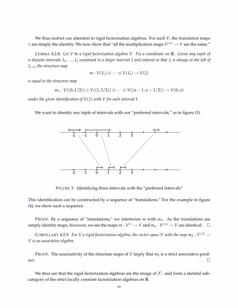
We thus restrict our attention to rigid factorization algebras. For such V , the translation mapsτ are simply the identity. We now show that “all the multiplication maps V⊗n → V are the same.”

LEMMA 4.2.8. Let V be a rigid factorization algebra V . Fix a coordinate on R. Given any tuple ofn disjoint intervals I1, . . . , In contained in a larger interval J and ordered so that Ij is always to the left ofIj+1, the structure map

m : V(I1)⊗ · · · ⊗ V(In)→ V(J)

is equal to the structure map

mn : V((0, 1/2))⊗ V((1, 3/2))⊗ · · · ⊗ V((n− 1, n− 1/2))→ V(0, n)

under the given identification of V(I) with V for each interval I.

We want to identify any tuple of intervals with our “preferred intervals,” as in figure (3).

0 1 2 3-1-2

0 1 2 3-1-2

FIGURE 3. Identifying three intervals with the “preferred intervals”

This identification can be constructed by a sequence of “translations.” For the example in figure(4), we show such a sequence.

PROOF. By a sequence of “translations,” we intertwine m with mn. As the translations aresimply identity maps, however, we see the maps m : V⊗ → V and mn : V⊗n → V are identical.

COROLLARY 4.2.9. For V a rigid factorization algebra, the vector space V with the map m2 : V⊗2 →V is an associative algebra.

PROOF. The associativity of the structure maps of V imply that m2 is a strict associative prod-uct.

We thus see that the rigid factorization algebras are the image of F− and form a skeletal sub-category of the strict locally constant factorization algebras on R.

65

0 1 2 3-1-2

0 1 2 3-1-2

0 1 2 3-1-2

0 1 2 3-1-2

FIGURE 4. A sequence of translations constructing the identification

4.3. Associative algebras and the bar complex

We have two goals here:

(1) to prove that the prefactorization algebra FA on R arising from an associative algebra Asatisfies the locality axiom;

(2) to relate the locality axiom for the factorization algebras on R to familiar constructionsfrom homological algebra, like derived tensor product and Hochschild homology.

The most useful result we’ll prove is the following.

PROPOSITION 4.3.1. For A a dg algebra, M a right A-module, and N a left A-module, let F(M,A,N)

the constructible prefactorization algebra on [0, 1] assigning M to every interval [0, x), N to every interval(x, 1], and A to every interval (x, y). It is a factorization algebra and its global sections are

F(M,A,N)([0, 1]) ' M⊗LA N.

Thus we can compute global sections using the bar complex.

0 1

AM N

FIGURE 5. The structure of FM,A,N

REMARK 4.3.2. For us, a constructible factorization algebra F on a space X means there is adecomposition X =

⊔i Xi into finitely many disjoint, locally closed subsets Xi, each of which is

66

a manifold, such that F∣∣

Xiis locally constant. Again, this is not the most general definition but

suffices for our purposes.

We build up to this result somewhat indirectly, by proving a result about tensor algebras (i.e.,free algebras) and then using resolutions.

PROPOSITION 4.3.3. For I an interval (with or without endpoints) and F be a cosheaf on I with valuesin dgVect, there is a factorization algebra TF on I such that for each open interval U,

TF(U) := T(F(U)) =∞⊕

n=0

F(U)⊗n.

In short, for an interval U, TF(U) is the tensor algebra of F(U).

As the proof of the proposition is unpleasantly long, we defer it to the end of the section andimmediately describe its consequences.

COROLLARY 4.3.4. Let V0f0← V

f1→ V1 be a diagram in dgVect. There is an associated constructiblecosheaf V on I = [0, 1] assigning V0 to every interval [0, x), V1 to every interval (x, 1], and V to everyinterval (x, y). The associated factorization algebra T = T(V) has global sections

T ([0, 1]) = T(V0)⊗T(V) T(V1).

In particular, given a vector space V, the locally constant prefactorization algebra FT(V) is, in fact, a factor-ization algebra.

We now use homological algebra to piggyback on proposition 4.3.3 to get a useful, generalresult. Recall that a semi-free algebra (R, d) is a dg algebra such that the underlying graded algebraR# is a tensor algebra.

LEMMA 4.3.5. For (R, d) a semi-free algebra, the locally constant prefactorization algebra FR is afactorization algebra.

PROOF. For any open U and any factorizing cover U, we need to show that the map

ι : C(U,FR)→ FR(U)

is a quasi-isomorphism. The Cech complex is naturally viewed as a double complex with hori-zontal differential given by the structure maps — for example, we have

F (α0, α1)d0−d1→ F (α0)⊕F (α1)

and so on — and the vertical differential given by the internal differential for each ~α. We canlikewise view the cone of ι as a double complex where we adjoin F (U) as the rightmost column.

Consider now the spectral sequence on this double complex Cone(ι) whose first page is givenby using the horizontal (i.e., Cech ) differential. We know the horizontal complex is acyclic byproposition 4.3.3, so the sequence vanishes on the first page.

67

COROLLARY 4.3.6. For (A, dA) a dg algebra, the locally constant prefactorization algebra FA is afactorization algebra.

PROOF. Pick a semi-free resolution (R, dR) of A. This means that (R, dR) is semi-free and thereis a surjective quasi-isomorphism q : R→ A.

We already know that FR is a factorization algebra. We also know that q induces a map ofprefactorization algebras q : FR → FA that is a quasi-isomorphism on every open. For any openU and any factorizing cover U, we thus have a commuting diagram

C(U,FR) //

FR(U)

C(U,FA) // FA(U)

where the top row and right column are quasi-isomorphisms. We now show that the left columnis a quasi-isomorphism via a spectral sequence.

Observe that there is a natural filtration of the Cech complex by “index.” Namely, let

FkC(U,F ) :=⊕n≤k

⊕~α∈PIn+1

F (~α).

The associated graded components are then

Fk/Fk−1 =⊕

~α∈PIk+1

F (~α).

Using this filtration, we see that the left column map induces a quasi-isomorphism on the firstpage of the spectral sequence because q : FR(~α) → FA(~α) is a resolution for every~α. Hence theleft column map is a quasi-isomorphism.

A parallel argument implies the following.

COROLLARY 4.3.7. For A a dg algebra, M a right A-module, and N a left A-module, let F(M,A,N)

the constructible prefactorization algebra on [0, 1] assigning M to every interval [0, x), N to every interval(x, 1], and A to every interval (x, y). It is a factorization algebra and its global sections are

F(M,A,N)([0, 1]) ' M⊗LA N.

Thus we can compute global sections using the bar complex.

Pushforward then implies a simple relationship with Hochschild homology.

COROLLARY 4.3.8. Parametrizing S1 by θ ∈ [0, 2π), we have a natural map p : S1 → [−1, 1]sending θ to cos θ. Then

FA(S1) = p∗FA([−1, 1]) ' A⊗LA⊗Aop A

as P∗FA is isomorphic to the factorization algebra F(A,A⊗Aop,A) on [−1, 1].

68

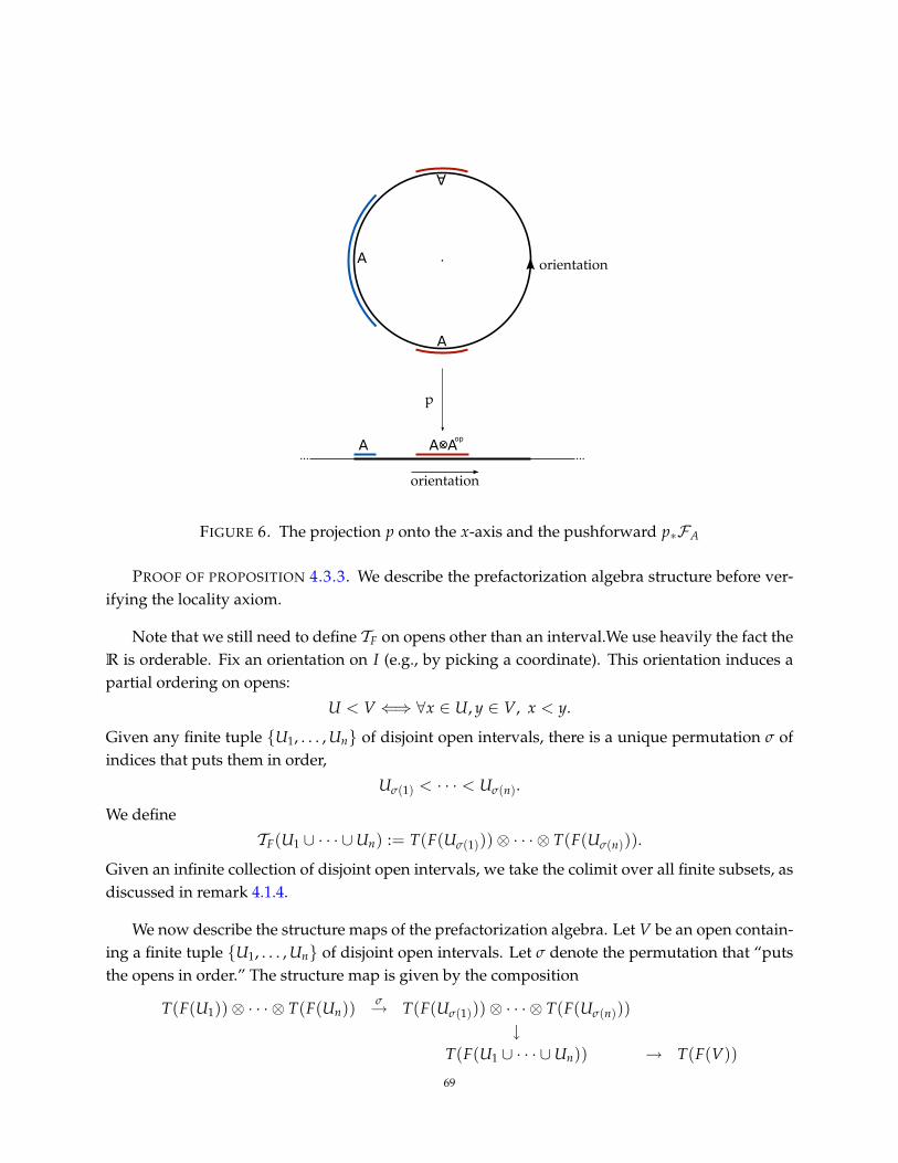
p

orientation

A

Aop

orientation

AA

A

A

FIGURE 6. The projection p onto the x-axis and the pushforward p∗FA

PROOF OF PROPOSITION 4.3.3. We describe the prefactorization algebra structure before ver-ifying the locality axiom.

Note that we still need to define TF on opens other than an interval.We use heavily the fact theR is orderable. Fix an orientation on I (e.g., by picking a coordinate). This orientation induces apartial ordering on opens:

U < V ⇐⇒ ∀x ∈ U, y ∈ V, x < y.

Given any finite tuple U1, . . . , Un of disjoint open intervals, there is a unique permutation σ ofindices that puts them in order,

Uσ(1) < · · · < Uσ(n).

We define

TF(U1 ∪ · · · ∪Un) := T(F(Uσ(1)))⊗ · · · ⊗ T(F(Uσ(n))).

Given an infinite collection of disjoint open intervals, we take the colimit over all finite subsets, asdiscussed in remark 4.1.4.

We now describe the structure maps of the prefactorization algebra. Let V be an open contain-ing a finite tuple U1, . . . , Un of disjoint open intervals. Let σ denote the permutation that “putsthe opens in order.” The structure map is given by the composition

T(F(U1))⊗ · · · ⊗ T(F(Un))σ→ T(F(Uσ(1)))⊗ · · · ⊗ T(F(Uσ(n)))

↓T(F(U1 ∪ · · · ∪Un)) → T(F(V))

69

where the first map uses the Koszul rule of signs to permute vectors and the third map is simplythe functor T (the free algebra functor) applied to the cosheaf structure map F(U1 ∪ · · · ∪Un) →F(V).

We now verify locality. Let U ⊂ I be an open and U = Vjj∈J be a factorizing cover of U. Weneed to prove that we have a quasi-isomorphism

C(U, TF) ' TF(U),

where C denotes the Cech complex from definition 4.1.6. (Our strategy mimics the proof of theo-rem 4.5.1 that Sym F is a factorization algebra.)

We introduce some notation to organize the combinatorics. Let U tV indicate that the union isof disjoint opens U and V. Given α ∈ PI := PI(J), set Uα := tj∈αVj. For~α = (α0, . . . , αN) ∈ PIN+1,set

U(~α) := ∩Ni=0Uαi .

Observe that we can swap intersections past unions to obtain

U(~α) = tj0∈α0,...,jN∈αN (∩Ni=0Vji),

because the opens ∩Ni=0Vji are pairwise disjoint. Thus, by the definition of TF, we have a natural

isomorphism

TF(~α) =⊗

j0∈α0,...,jN∈αN

TF(∩Ni=0Vji) ∼= TF(U(~α)),

where the isomorphism “puts the components in order.”

Under this isomorphism, the structure maps preserve tensor power and hence so does thedifferential in the Cech complex, as we now explain. By “tensor power,” we mean that an elementw ∈ V⊗n ⊂ T(V) is of tensor power n. Observe that for a disjoint union U tU′ with U < U′, wecan view TF(U tU′) = T(F(U))⊗ T(F(U′)) as a vector subspace of T(F(U tU′)). For w⊗ w′ ∈TF(U tU′), with w of tensor power n and w′ of tensor power n′, the image in T(F(U tU′)) hastensor power n + n′. On every open U, we equip TF(U) with this natural “total grading” by tensorpower and write TF(U) =

⊕n≥0 TF(U)〈n〉, where the superscript 〈n〉 indicates the subspace with

grading 〈n〉.

Decompose the Cech complex into a sum of complexes over tensor power. It now remains toshow that

(†) colim

(· · · →

⊕~α∈PI2

TF(U(~α))〈n〉 →⊕

α

TF(Uα)〈n〉)→ TF(U)〈n〉

is a quasi-isomorphism for every n.

70

Our method is to relate T 〈n〉F to Fn, the cosheaf on the product space In = I × · · · × I︸ ︷︷ ︸n times

given by

the n-fold external tensor product of F. In particular, we define a subset U〈n〉 ⊂ In for each openU ⊂ I such that F(U〈n〉) = T 〈n〉F (U).

DEFINITION 4.3.9. For U ⊂ I, there is a unique decomposition U = tj∈J Ij, where the Ij aredisjoint open intervals. The index set J is totally ordered by the relation that j < j′ if Ij < Ij′ . Let[n] := 0 < 1 < · · · < n− 1 denote the model totally ordered set with n elements. We define

J〈n〉 := f : [n]→ J : f (0) ≤ f (1) ≤ · · · ≤ f (n− 1) .

In other words, J〈n〉 consists of the monotonically increasing functions from [n] into J. For f ∈ J〈n〉,we define

U f :=n−1

∏i=0

I f (i) ⊂ In.

Finally, we define

U〈n〉 :=⊔

f∈J〈n〉U f .

Note that this is a disjoint union of connected opens.

This definition is the bridge between T 〈n〉F and Fn.

LEMMA 4.3.10. For every open U ⊂ I, we have TF(U)〈n〉 = Fn(U〈n〉).

PROOF OF LEMMA. We compute

Fn(U〈n〉) = Fn(⊔

f∈J〈n〉U f )

=⊕

f∈J〈n〉Fn(U f )

=⊕

f∈J〈n〉

n−1⊗i=0

F(I f (i))

= TF(U)〈n〉.

For the last step, recall that TF(U) =⊗

j∈J T(F(Ij)).

We claim that the cosheaf gluing axiom for Fn implies the desired quasi-isomorphism (†).Suppose the following facts, which we will prove below:

(1) the opens U〈n〉α α∈PI form a cover for U〈n〉, and(2) U〈n〉α ∩U〈n〉β = (Uα ∩Uβ)〈n〉 for all α, β.

71

By assertion (2), we see that for any~α ∈ PIN+1, we have U(~α)〈n〉 =⋂N

i=0 U〈n〉αi . In the diagram (†),we replace every T 〈n〉F (U(~α)) with F(

⋂Ni=0 U〈n〉αi ). We then obtain the diagram

colim

· · · → ⊕(α0,α1)∈PI2

Fn(U〈n〉α0 ∩U〈n〉α1 )→⊕

α

Fn(U〈n〉α )

→ Fn(U〈n〉)

This is precisely the cosheaf Cech diagram for Fn on U〈n〉 using the cover U〈n〉α α∈PI . As thisdiagram holds, we obtain the locality axiom.

It remains to verify assertions (1) and (2).

We know (1) by the factorizing property of the basis U. Given any point x = (x1, . . . , xn) ∈U〈n〉, there exists α ∈ PI such that x1, . . . , xn ∈ Uα, and so x ∈ U〈n〉α .

We obtain (2) as a consequence of a more general fact.

LEMMA 4.3.11. Let U and V be open subsets of I. Then U〈n〉 ∩V〈n〉 = (U ∩V)〈n〉 for any n.

PROOF OF LEMMA. Let U = tj∈JUj and V = tk∈KVk be the unique decompositions into openintervals. Both J and K are totally ordered by the orientation of I. Then

U ∩V =⊔

(j,k)∈L

Uj ∩Vk,

where

L := (j, k) ∈ J × K : Uj ∩Vk 6= ∅.

Note that L also obtains a total ordering from the orientation of the interval I.

Note that L〈n〉 → J〈n〉 × K〈n〉 because h(i) ∈ J × K for every i ∈ [n].

Given ( f , g) ∈ J〈n〉 × K〈n〉, we compute

U f ∩Vg =n

∏i=0

(U f (i) ∩Vg(i)),

because the cartesian product commutes with intersections. Hence U f ∩ Vg 6= ∅ if and only if( f , g) ∈ L〈n〉.

72

Thus we see

U〈n〉 ∩V〈n〉 =

⊔f∈J〈n〉

U f

∩ ⊔

g∈K〈n〉Vg

=

⊔( f ,g)∈J〈n〉×K〈n〉

U f ∩Vg

=⊔

( f ,g)∈L〈n〉U f ∩Vg

= (U ∩V)〈n〉,

which is what needed to be proved.

Thus (2) follows directly from the lemma.

4.4. The category of factorization algebras

In this section, we explain how prefactorization algebras and factorization algebras form cat-egories. In fact, they naturally form multicategories (or colored operads). We also explain howthese multicategories are enriched in simplicial sets when the (pre)factorization algebras take val-ues in cochain complexes.

4.4.1. Morphisms and the category structure.

DEFINITION 4.4.1. A morphism of prefactorization algebras φ : F → G consists of a mapφU : F(U) → G(U) for each open U ⊂ M, compatible with the structure maps. That is, for anyopen V and any finite collection U1, . . . , Uk of pairwise disjoint open sets, each contained in V, thefollowing diagram commutes:

F(U1)⊗ · · · ⊗ F(Uk)φU1⊗···⊗φUk−→ G(U1)⊗ · · · ⊗ G(Uk)

↓ ↓F(V)

φV−→ G(V)

Likewise, all the obvious associativity relations are respected.

REMARK 4.4.2. When our prefactorization algebras take values in cochain complexes, we re-quire the φU to be cochain maps, i.e., they each have degree 0 and commute with the differentials.

DEFINITION 4.4.3. On a space X, we denote the category of prefactorization algebras on Xtaking values in the symmetric monoidal category C by PreFA(X, C). The category of factorizationalgebras, FA(X, C), is the full subcategory whose objects are the factorization algebras.

Throughout the thesis, we will want to say when two (pre)factorization algebras are equiva-lent. Here are two notions we use repeatedly.

73

DEFINITION 4.4.4. A morphism φ : F → G of prefactorization algebras (with values in dgVect)is a quasi-isomorphism if it is a quasi-isomorphism on every open. It is an opens-wise homotopyequivalence if on each open U, the morphism φ(U) : F(U) → G(U) extends to a chain homo-topy equivalence, though we do not require compatibility between the structure maps and theequivalences.

REMARK 4.4.5. A full theory of factorization algebras would encompass good notions of equiv-alence, a characterization of FA as a localization of PreFA (hopefully), and much more. We makeno pretensions to providing such a theory in this text. The notion of opens-wise homotopy equiv-alence, for instance, is not even an equivalence relation. It just happens to be a stronger propertythan quasi-isomorphism that we can verify explicitly in several cases.

N.B. 4.4.6. Even if these notions were well-behaved, we are often working with cochain com-plexes of topological vector spaces, a notoriously awkward setting. Homological algebra and topo-logical vector space mix uneasily, and in [CG] we are pursuing an alternative with diffeologicalspaces. In this thesis, we will usually either explicitly construct continuous homotopy equivalences(e.g., with the Atiyah-Bott lemma, see lemma 5.2.13) or work with complexes whose cohomologyis well-behaved topologically.

4.4.2. The multicategory structure. There is a natural tensor product on PreFA(X, C), as follows.Let F, G be prefactorization algebras. We define F⊗ G by

F⊗ G(U) := F(U)⊗ G(U),

and we simply define the structure maps as the tensor product of the structure maps. For instance,if U ⊂ V, then the structure map is

F(U ⊂ V)⊗ G(U ⊂ V) : F⊗ G(U) = F(U)⊗ G(U)→ F(V)⊗ G(V) = F⊗ G(V).

DEFINITION 4.4.7. Let PreFAmc(X, C) denote the multicategory arising from the symmetricmonoidal product on PreFA(X, C). That is,

PreFAmc(F1, · · · , Fn; G) := PreFA(F1 ⊗ · · · ⊗ Fn, G).

Factorization algebras inherit this multicategory structure.

4.4.3. Enrichment over simplicial sets. Recall that cochain complexes are enriched over simpli-cial sets as follows. For K a simplicial set,

sSets(K, Maps(A, B)) = dgVect(A, Ω∗(K)⊗ B),

where dgVect(A, B) denotes the cochain maps, i.e., degree zero maps that commute with the dif-ferentials, and Ω∗(K) denotes the de Rham complex on the geometric realization of K. In partic-ular, the n-simplices of Maps(A, B) are precisely dgVect(A, Ω∗(∆n) ⊗ B). Let dgVect denote the

74

category whose objects are cochain complexes and whose morphisms from A to B is the mappingspace Maps(A, B). This category is enriched over simplicial sets.

We use this same method to enrich prefactorization algebras over simplicial sets. Given pref-actorization algebras F, G taking values in cochain complexes, define Maps(F, G) as follows. Ann-simplex φ in Maps(F, G) consists of a map φU ∈ dgVect(F(U), Ω∗(∆n)⊗ G(U)) for each openU ⊂ X, compatible with the structure maps.

4.4.4. Factorization algebras with structures.

DEFINITION 4.4.8. A commutative factorization algebra F with values in C⊗ is

(1) a prefactorization algebra taking values in CAlg(C), the category of commutative alge-bras in C with the usual tensor product ⊗ as the symmetric monoidal structure;

(2) a factorization algebra in C after applying the forgetful functor to C on every open.

By theorem 4.5.1 below, the factorization algebra SymF of a cosheaf F is a commutative fac-torization algebra.

4.5. General construction methods for factorization algebras

Generating prefactorization algebras is fairly easy but verifying the locality axiom is nontrivial,so it is convenient to have procedures that provide examples. Sometimes these examples areboring in themselves, but we obtain nontrivial factorization algebras by deforming them. BVquantization, for instance, is a systematic procedure for finding meaningful deformations. In thissection, we introduce two sources of factorization algebras, one using commutative algebras andthe other Lie algebras.

THEOREM 4.5.1. For every cosheaf of dg vector spaces F , the precosheaf SymF is a factorizationalgebra. Moreover, Sym defines a functor from cosheaves to factorization algebras.

PROOF. It is straightforward to show that SymF is a prefactorization algebra. We simply needto obtain the structure maps. Note that for a finite collection of disjoint opens U1, . . . , Uk, there isa canonical isomorphism

F (U1 ∪ · · · ∪Uk) ∼= F (U1)⊕ · · · ⊕ F (Uk)

and hence a canonical isomorphism

SymF (U1 ∪ · · · ∪Uk) ∼= SymF (U1)⊗ · · · ⊗ SymF (Uk).

Thus, if the opens are all contained in the open V, we get the structure map

SymF (U1)⊗ · · · ⊗ SymF (Uk) ∼= SymF (U1 ∪ · · · ∪Uk)→ SymF (V).

75

The coherences of the cosheaf induce those for the prefactorization algebra.

We now verify the locality axiom.

Our first reduction is to observe that all the structure maps preserve the “algebraic degree”:that is, the structure map above is simply the direct sum over m of the maps

Symm F (U1 ∪ · · · ∪Uk)→ Symm F (V).

Thus, it suffices to verify the locality axiom independently for each m.

Explicitly, that means the following. For each α ∈ PI, let Uα = äi∈α Ui. Note that

SymF (α, β) =⊗

i∈α,j∈β

SymF (Ui ∩Uj) ∼= SymF (Uα ∩Uβ),

and likewise for the case with α0, . . . , αn. The Symm level of the locality axiom becomes the re-quirement that

colim(· · · → ⊕α,β∈PI Symm F

(Uα ∩Uβ

)→ ⊕γ∈PI Symm F (Uγ)

)→ Symm F (U)

is a quasi-isomorphism.

Second, observe thatF (U)⊗m = Fm(Um)

where Fm is the cosheaf on Um = U × · · · ×U︸ ︷︷ ︸m times

obtained as the external product of F with itself

m times.

Thus it is enough to show that

Fm(Um) = colim(· · · → ⊕α,β∈PIFm ((Uα ∩Uβ)m)→ ⊕γ∈PIFm (Um

γ

)).

Our cover U is a factorizing cover. This means that, for every finite set of points x1, . . . , xk ∈ Mwe can find disjoint open subsets Ui1 , . . . , Uik in the cover U with xi ∈ Uii . This implies that thesubsets of Um of the form (Uα)m, where α ∈ PI, cover Um. Further,

(Uα)m ∩ (Uβ)m = (Uα ∩Uβ)m.

The desired isomorphism now follows from the fact that Fm is a cosheaf on Mm.

Every morphism of cosheaves clearly induces a morphism of prefactorization algebras, andhence factorization algebras.

Now we consider the Lie-theoretic method.

DEFINITION 4.5.2. A Lie-structured cosheaf of vector spaces g is a precosheaf of dg Lie algebrasthat is a cosheaf of dg vector spaces (after applying the forgetful functor Forget : dgLie→ dgVect).

We have two favorite examples of Lie-structured cosheaves: let g be a dg Lie algebra, then

76

(1) define gM := Ω∗M,c⊗ g to be the cosheaf of compactly-supported, g-valued de Rham formson a smooth manifold M;

(2) define gM∂ := Ω0,∗M,c ⊗ g be the cosheaf of compactly-supported, g-valued Dolbeault forms

on a complex manifold M.

Both these examples will reappear throughout the text.

THEOREM 4.5.3. For every Lie-structured cosheaf g, applying the functor of Chevalley-Eilenbergchains C∗g to each open

U 7→ (Sym(g(U)[1]), dCE)

is a factorization algebra in dg vector spaces. We denote this factorization algebra by C∗g. Moreover C∗defines a functor from Lie-structured cosheaves to factorization algebras.

We call C∗g the enveloping factorization algebra of g.

REMARK 4.5.4. Every cosheaf of dg vector spaces is a Lie-structured cosheaf where we assignan abelian dg Lie algebra to each open. Hence this theorem is a very direct generalization oftheorem 4.5.1.

PROOF. Consider the filtration on the prefactorization algebra

FiC∗g := Sym≤i(g[1]).

We will use the spectral sequence induced by this filtration to show C∗(g) is a factorization algebra.For any factorizing cover U of an open U, the structure maps induce a map

C(U, C∗g)→ C∗g(U)

and hence a map of spectral sequences. The first page of these spectral sequences is given by for-getting the Lie algebra structure on g and simply viewing g[1] as a cosheaf in dg vector spaces andthen applying the functor Sym. Hence by theorem 4.5.1 the map on the first page is an isomor-phism. The original map is thus a quasi-isomorphism.

REMARK 4.5.5. For the manifold Rn, the factorization algebra C∗gRnprovides the En enveloping

algebra of g. In the next section, we prove a shadow of this assertion by showing that for g a gradedLie algebra, C∗gR recovers the universal enveloping algebra (i.e., the E1 enveloping algebra) Ug

of g. To prove the full assertion, one needs to use the full power of ∞-categories and homotopicalalgebra, which is far beyond our scope. A proof should follow quite directly from results in [Lurb]and [Fra]. We now sketch the idea with no pretense of rigor.

Recall that the formality of the En operad in characteristic zero states that the En operad isequivalent to the Pn operad (i.e., the operad describing commutative dg algebras with a Poissonbracket of degree 1− n). There is a forgetful functor from Pn algebras to dg Lie algebras by forget-ting the commutative product and shifting the complex down by n− 1. There is an adjoint to thisforgetful functor, giving the “enveloping” Pn algebra of a dg Lie algebra. Explicitly, the enveloping

77

Pn algebra of (g, d) is (Sym(g[1− n]), d) where we extend d as a derivation and extend the shiftedbracket of g to obtain the Poisson bracket. Formality then tells us that we can lift the envelopingPn algebra to an En algebra.

A simple computation shows that C∗gRn, when viewed as an En algebra, has the correct com-

mutative product and shifted Lie bracket. In particular, consider the structure map given by theinclusion of a small n-disk nested inside a thickened n− 1-sphere into a large n-disk. This struc-ture map encodes the shifted Lie bracket.

4.6. A novel construction of the universal enveloping algebra

Let g be a graded Lie algebra (i.e., a dg Lie algebra with zero differential). Recall that gR

denotes the Lie-structured cosheaf on R that assigns (Ω∗c (U) ⊗ g, d) to each open U, with d theexterior derivative. Our main result shows how to construct the universal enveloping algebra Ug

using theorem 4.5.3.

PROPOSITION 4.6.1. Let H denote the cohomology prefactorization algebra of C∗gR, the envelopingfactorization algebra of gR. That is, we take the cohomology of every open and every structure map, so

H(U) = H∗(C∗gR(U))

for any open U. ThenH is isomorphic to FUg, the factorization algebra for the universal enveloping algebraof g.

We break the proof into a sequence of lemmas. First, we obtain a kind of PBW result (showingthe proposition is plausible).

LEMMA 4.6.2. On an open interval U, the vector space H(U) has a natural filtration F such thatGrFH(U) ∼= Sym g.

PROOF. Let F denote the filtration on C∗gR(U) where Fk = Sym≤k(gR(U)[1]). Then F is theinduced filtration on its cohomologyH(U). Now consider the spectral sequence induced by F. Itsfirst page is the cohomology of the complex (Sym(gR(U)[1]), ddR), with ddR the exterior derivative.This cohomology is precisely Sym g, by the compactly-supported Poincare lemma.

For g an ordinary Lie algebra (i.e., concentrated in degree 0), we see the spectral sequencecollapses because the first page is concentrated in degree 0.

For g a graded Lie algebra, we see that the differential vanishes on every higher page as fol-lows. For any nontrivial element on the first page, a lift to C∗gR(U) lives in Sym(Ω1(U) ⊗ g).The full differential vanishes on any such element because the wedge of two 1-forms is alwayszero.

Now we showH is locally constant and hence corresponds to some associative algebra A.

78

LEMMA 4.6.3. For any inclusion i : U ⊂ V of an interval into an interval, the associated structuremapH(i) ofH is an isomorphism. HenceH is a locally constant factorization algebra.

PROOF. Apply the filtration from the previous lemma to obtain a morphism of spectral se-quences. We know that i! (extension by zero) induces a quasi-isomorphism from Ω∗c (U) to Ω∗c (V),so this morphism of spectral sequences is an isomorphism on the first page. Thus the structuremap

C∗gR(i) : C∗gR(U)→ C∗gR(V)

is a quasi-isomorphism, implying the lemma.

Together, these lemmas imply that A is isomorphic to Sym g as a vector space. We wish toshow that g generates A as an algebra. To make this precise, we introduce some notation thatallows us to define an inclusion map ιU : g→ H(U) for each interval U.

Pick a bump function φ on R such that

• φ ≥ 0;• supp(φ) ⊂ (0, 1);•∫

Rφ(t) dt = 1.

To each interval U = (a, b), we then associate the 1-form

αU :=U

b− aφ

(t− ab− a

)dt,

which has support in U and integrates to 1, by construction. Observe that for any X ∈ g, theelement αU ⊗ X is a cocycle in C∗gR(U) whose cohomology class [αU ⊗ X] goes to X in GrFH(U).Define ιU by X 7→ [αU ⊗ X]. Note that for an inclusion i : U ⊂ V of intervals, we have ιV =H(i) ιU by construction. Thus there is a well-defined map ι : g→ A.

LEMMA 4.6.4. Viewing g as the image of ι, it generates the algebra A.

PROOF. Let Xν := X1X2 · · ·Xn be an arbitrary element of Symn g. We will use ι to obtain anelement Ξ in A whose image in GrF A is precisely this element Xν.

Pick an interval U and a collection of subintervals

U1 < U2 < · · · < Un.

(Recall from section 4.3 that I < J if every element of I is less than every element of J.) Considerthe element

ιU1(X1)⊗ · · · ⊗ ιUn(Xn) ∈ H(U1)⊗ · · · ⊗H(Un)

and apply the structure map

m : H(U1)⊗ · · · ⊗H(Un)→ H(U)

79

to obtain a representative for Ξ (under the identification between H(U) and A). At the cochainlevel, we have

(αU1 ⊗ X1)⊗ · · · ⊗ (αUn ⊗ Xn) ∈ C∗gR(U1)⊗ · · · ⊗ C∗gR(Un).

Under the analogous structure map for C∗gR, we view (αU1 ⊗ X1) ⊗ · · · ⊗ (αUn ⊗ Xn) as an ele-ment of Symn(Ω1

c(U)⊗ g) by extending the forms αUj by zero. This element is closed and hencedescends to some cohomology class. Using the filtration/spectral sequence from earlier, we seethat it corresponds precisely to Xν.

We now show that these generators satisfy the same relations as Ug. Let • denote multiplica-tion in A.

LEMMA 4.6.5. For all X, Y ∈ g, we have the following relation in A:

ι(X) • ι(Y)− ι(Y) • ι(X) = ι([X, Y]).

Thus A is isomorphic to Ug.

PROOF. We will obtain this relation by showing that the elements on either side of the equalityrepresent the same cohomology classes. Thus, we work at the cochain level (i.e., in C∗gR).

Pick intervals U1 < U2 < U3 inside a bigger interval V. Let m denote the structure map

C∗gR(U1)⊗ C∗gR(U2)⊗ C∗gR(U3)→ C∗gR(V).

We want to compute

m((αU1 ⊗ X)⊗ (αU2 ⊗Y)⊗ 1)−m(1⊗ (αU2 ⊗Y)⊗ (αU3 ⊗ X))

and see that it is cohomologous to αU2 ⊗ [X, Y]. This implies the relation for H, at the level ofcohomology.

Let

Φ(t) =∫ t

−∞αU1 −

∫ t

−∞αU3

denote a compactly supported function on V. Consider the element Φ⊗X · αU2⊗Y in Sym2(Ω∗c (V)⊗g[1]). We compute

dC∗(Φ⊗ X · αU2 ⊗Y) = (ddRΦ)⊗ X · αU2 ⊗Y−ΦαU2 ⊗ [X, Y]

= αU1 ⊗ X · αU2 ⊗Y− αU3 ⊗ X · αU2 ⊗Y− αU2 ⊗ [X, Y]

= αU1 ⊗ X · αU2 ⊗Y− αU2 ⊗Y · αU3 ⊗ X− αU2 ⊗ [X, Y]

since Φ∣∣U2≡ 1 and all the elements are cohomologically degree 0. Hence, inH(V), we see that

X •Y−Y • X− [X, Y] = 0,

as it is a boundary.

80

REMARK 4.6.6. In chapter 6 on vertex algebras, we will use a variant of this construction for Σa Riemann surface to construct the Kac-Moody vertex algebras.

4.7. Extension from a factorizing basis

4.7.1. Factorization algebras defined on a factorizing basis. Let X be a topological space, and letU be a basis for X, which is closed under taking finite intersections. It is well-known that there isan equivalence of categories between sheaves on X and sheaves which are only defined for opensets in the basis U. In this section we will prove a similar statement for factorization algebras. Thiswill allow us to perform several useful formal constructions with factorization algebras, such asgluing.

DEFINITION 4.7.1. A factorizing basis for X is a basis U of open sets of X which is closed underfinite intersections and is also a factorizing cover for X.

Let U be a factorizing basis.

DEFINITION 4.7.2. A U-prefactorization algebra F is like a factorization algebra, except thatF (U) is only defined for U ∈ U. A U-factorization algebra is a U-prefactorization algebra with theproperty that, for all U ∈ U and all factorizing covers V of U consisting of open sets in U,

C(V,F ) ' F (U),

where C(V,F ) denotes the Cech complex described earlier in section 4.1.

In this section we will show that any U-factorization algebra on X extends to a factorizationalgebra on X. This extension is unique up to quasi-isomorphism.

Let F be a U-factorization algebra. Let us define a prefactorization algebra iU∗F on X by

iU∗ (F )(V) = C(UV ,F ),

for each V ⊂ X open. Here UV is the cover of V consisting of those open subsets in the cover U

which are contained in V.

LEMMA 4.7.3. With this definition, iU∗ (F ) is a factorization algebra whose restriction to open sets inthe cover U is quasi-isomorphic to F .

PROOF. We need to check that if W is a factorizing cover of V ⊂ X, then

iU∗ (F )(V) ' C(W, iU∗ (F )).

Before we prove this, we need a lemma. Let UW be the cover of V consisting of open sets in U

which are subordinate to W.

81

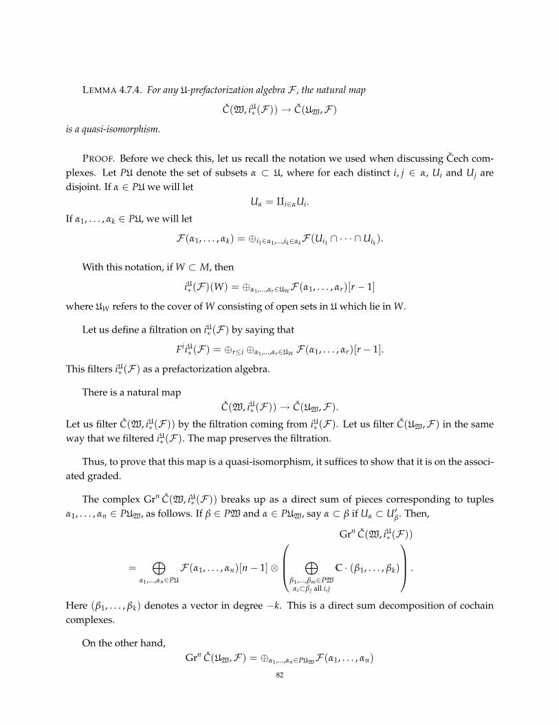
LEMMA 4.7.4. For any U-prefactorization algebra F , the natural map

C(W, iU∗ (F ))→ C(UW,F )

is a quasi-isomorphism.

PROOF. Before we check this, let us recall the notation we used when discussing Cech com-plexes. Let PU denote the set of subsets α ⊂ U, where for each distinct i, j ∈ α, Ui and Uj aredisjoint. If α ∈ PU we will let

Uα = qi∈αUi.

If α1, . . . , αk ∈ PU, we will let

F (α1, . . . , αk) = ⊕i1∈α1,...,ik∈αkF (Ui1 ∩ · · · ∩Uik).

With this notation, if W ⊂ M, then

iU∗ (F )(W) = ⊕α1,...,αr∈UWF (α1, . . . , αr)[r− 1]

where UW refers to the cover of W consisting of open sets in U which lie in W.

Let us define a filtration on iU∗ (F ) by saying that

FiiU∗ (F ) = ⊕r≤i ⊕α1,...,αr∈UW F (α1, . . . , αr)[r− 1].

This filters iU∗ (F ) as a prefactorization algebra.

There is a natural mapC(W, iU∗ (F ))→ C(UW,F ).

Let us filter C(W, iU∗ (F )) by the filtration coming from iU∗ (F ). Let us filter C(UW,F ) in the sameway that we filtered iU∗ (F ). The map preserves the filtration.

Thus, to prove that this map is a quasi-isomorphism, it suffices to show that it is on the associ-ated graded.

The complex Grn C(W, iU∗ (F )) breaks up as a direct sum of pieces corresponding to tuplesα1, . . . , αn ∈ PUW, as follows. If β ∈ PW and α ∈ PUW, say α ⊂ β if Uα ⊂ U′β. Then,

Grn C(W, iU∗ (F ))

=⊕

α1,...,αn∈PU

F (α1, . . . , αn)[n− 1]⊗

⊕β1,...,βm∈PWαi⊂β j all i,j

C · (β1, . . . , βk)

.

Here (β1, . . . , βk) denotes a vector in degree −k. This is a direct sum decomposition of cochaincomplexes.

On the other hand,Grn C(UW,F ) = ⊕α1,...,αn∈PUW

F (α1, . . . , αn)

82

Thus, to prove the lemma, we need to verify that the complex

⊕β1,...,βm∈PWαi⊂β j all i,j

C · (β1, . . . , βk)

has homology C if all αi ∈ PUW, and zero otherwise.

It is clear that the complex is zero if all αi are not in PUW. So let us assume that all αi arein PUW. Then, the complex is simply the simplicial chain complex on the infinite simplex withvertices β ∈ PU such that ∪Uαi ⊂ Uβ. This is of course contractible.

It remains to shows that the natural map

C(UW,F )→ C(UV ,F )

is a quasi-isomorphism. (Here, as before, UV refers to the cover of V consisting of sets in U whichlie in V).

To see that this map is a quasi-isomorphism, observe that by another application of the sub-lemma there is a quasi-isomorphism

C(U, iUW∗ (F )) ' C(UW,F ).

Here iUW∗ refers to the prefactorization algebra on V obtained by extending F , as before, but nowconsidered as a UW-factorization algebra.

Now the fact that F is a U-factorization algebra implies that, for all U ∈ U, the natural map

C(UW ∩ UU ,F )→ F (U)

is a quasi-isomorphism.

It follows that the natural map

C(U, iUW∗ (F ))→ C(U,F )

is a quasi-isomorphism, as desired.

4.8. Pushforward and Pullback

So far, we have only discussed factorization algebras on a fixed manifold M. It is useful tounderstand how factorization algebras can be moved between spaces along a smooth map f :M → N. Just as with sheaves, pushforwards are straightforward. Pullbacks, however, are moresubtle and are only easily constructed when f is an embedding.

83

4.8.1. Pushing forward factorization algebras. A crucial feature of factorization algebras is thatthey push forward nicely. Let M and N be topological spaces admitting factorizing covers andlet f : M → N be a continuous map. Given a factorizing cover U = Uα of an open U ⊂ N,let f−1U = f−1Uα denote the preimage cover of f−1U ⊂ M. Observe that f−1U is factorizing:given a finite collection of points x1, . . . , xn in f−1U, the image points f (x1), . . . , f (xn) canbe covered by a disjoint collection of opens Uα1 , . . . , Uαk in U and hence f−1Uα1 , . . . , f−1Uαk is adisjoint collection of opens in f−1U covering the xj.

DEFINITION 4.8.1. Given a factorization algebra F on a space M and a continuous map f :M→ N, the pushforward factorization algebra f∗F on N is defined by

f∗F (U) := F ( f−1(U)).

Note that for the map to a point f : M → pt, the pushforward factorization algebra f∗Fis simply the global sections of F . We also call this the factorization homology of F on M. Wesometimes denote this FH(M,F ).

REMARK 4.8.2. It can be convenient to compute sheaf cohomology by iterating pushforwards.For instance, the Serre spectral sequence computes the sheaf cohomology on the total space of afiber bundle by first pushing forward the sheaf to the base space and then pushing forward to apoint. Likewise, it can be helpful to compute factorization homology by iterating pushforwardsand thus obtaining spectral sequences.

4.8.2. A case where pushforwards commute. The notion of pushforward intertwines nicely withour general construction methods.

PROPOSITION 4.8.3. Let g be a Lie-structured cosheaf on a topological space M. Let f : M → N be acontinuous map. Then the factorization algebra C∗( f∗g) is naturally isomorphic to f∗(C∗g).

PROOF. On an open U ⊂ N,

C∗( f∗g)(U) = C∗(g( f−1(U))) = f∗(C∗g)(U).

Likewise, the structure maps are identical.

4.8.3. Pulling back factorization algebras. Let F be a factorization algebra on M. Let U ⊂ M bean open subset. Then we can restrict F to a factorization algebra F

∣∣U on U, whose value on an

open subset V ⊂ U is simply F (V).

In this section we will discuss a generalization of this construction. We will not try to definepull-backs for arbitrary maps, but only for open immersions.

84

Let f : N → M be an open immersion. Let U f be the cover of N consisting of those opensubsets U ⊂ N with the property that

f |U : U → f (U)

is a homeomorphism. (To say that f is an open immersion means that sets of this form cover N).

Now, U f is a factorizing basis for N. Let us define a U f -prefactorization algebra f ∗F by

f ∗F (U) = F ( f (U))

if U ∈ U f .

LEMMA 4.8.4. f ∗F is a U f -factorization algebra.

PROOF. We need to verify that if U ∈ U f , and V is a factorizing cover of U by elements of U f ,that

C(V, f ∗F ) ' f ∗F (U) = F ( f (U)).

Now, f (V) is a factorizing cover of f (U), and

C(V, f ∗F ) = C( f (V,F ).

The result follows from the fact that F is a factorization algebra on M.

So far we have defined f ∗F as a U f -factorization algebra. We can extend (see section 4.7) f ∗Fto an actual factorization algebra, which we will continue to call f ∗F .

85

CHAPTER 5

Free fields and their observables

5.1. Introduction

In this chapter we will show how the viewpoint of BV quantization articulated in chapter 2carries over precisely to one class of field theories. These are the simplest kind of field theories —what we’ll call the free theories — and most interesting field theories (such as Chern-Simons, Yang-Mills, or even φ4) do not fall into this class. Nonetheless, they play a special role in perturbativeQFT because every interacting theory is studied as a deformation of a free theory. It thus behoovesus to obtain an understanding of free theories that is as clear and thorough as possible. Moreover,many mathematical structures that appear complicated or obscure in the interacting cases haveclean, elegant interpretations in the free setting. For instance, we’ll see familiar constructions likedeterminants of complexes and Heisenberg Lie algebras appear quite naturally in this context.One reason behind this relative simplicity is that we use only basic homological algebra and anal-ysis for free fields; Feynman diagrams and other constructions from physics do not appear, whichmakes free fields particularly accessible to a mathematician. Indeed, one goal of this thesis is tosee exactly how much one can accomplish without requiring the full machinery of perturbativefield theory developed in, for instance, [Cos11].

Before embarking on the myriad definitions and constructions that constitute this chapter, wequickly discuss what field theory is and then overview what’s accomplished in this chapter.

5.1.1. Classical field theory and deformations. Field theory has two aspects — the classical andthe quantum — and classical field theory is essentially (a subset of) the study of partial differentialequations. In practice, the equations studied in field theory usually arise from variational prob-lems and hence are the Euler-Lagrange equations of some action functional. Understanding thespaces of solutions of a PDE is often quite difficult. Perturbative classical field theory, from ourviewpoint (see [CG]), consists of studying the formal neighborhood of a fixed solution to a PDEin the moduli space of all solutions, and hence we describe the formal moduli space by a dg Liealgebra (or L∞ algebra), following the correspondence

formal moduli problems ↔ dg Lie algebras

that is well-established in deformation theory. (We elaborate on this assertion in the next para-graph below.) We thus obtain the following dictionary between terminology in field theory (physics),PDE, and deformation theory (using the correspondence above):

87

physics PDE Lie theoryfree theory linear system abelian dg Lie algebrainteracting theory nonlinear system nonabelian dg Lie algebra

It should be clear that free theories ought to be substantially simpler to understand.

5.1.2. An example. An example is in order, and we use the original motivating example: moduliof flat connections. Let M be a smooth manifold with a vector bundle E → M and a flat connec-tion ∇. We want to study infinitesimal deformations of the connection ∇, where we only wantdeformations that are also flat. The space of all connections on E is simply Ω1(End E), where weidentify the origin of this vector space with ∇. The space of flat connections is the subspace

A ∈ Ω1(End E) : (∇+ A)2 = 0

,

although we should take into account the gauge-equivalence of different connections (i.e., howautomorphisms of the bundle relate the connections). In summary, we want to describe the formalneighborhood of the origin up to gauge equivalence.

The flat connection ∇ on E induces a flat connection on End E, which we abusively denote ∇as well. Consider the de Rham complex of End E

g := (Ω∗(End E),∇).

This sheaf naturally takes values in dg Lie algebras via the usual bracket on endomorphisms. TheMaurer-Cartan equation in this situation is simply

∇A +12[A, A] = 0,

with A ∈ Ω1(End E), which is precisely the zero-curvature equation given earlier. Because weare interested in the formal moduli problem, however, we will focus on A that are “infinitesimal.”Thus, we consider the functor

Def∇ : dgArt→ sSets

sending a local dg Artinian ring (R, m) to the simplicial set Def∇(R)• whose n-simplices are

MC(g⊗m⊗Ω∗(∆n)),

which denotes families over the n-simplex ∆n of solutions to the Maurer-Cartan equation in g⊗m.Explicitly, if A is a degree 1 element of Ω∗(End E)⊗m⊗Ω∗(∆n), then the Maurer-Cartan equationis

∇A + dR A + ddR A +12[A, A] = 0,

where dR is the derivation on R and ddR denotes the exterior derivative on the de Rham forms onthe n-simplex. Although it looks complicated at first, this functor Def∇ is a natural construction.It encodes, for instance, all the infinitesimal deformations of ∇ (these are the 0-simplices) andhow these deformations are related by gauge transformations (or, more accurately, homotopies— these are the 1-simplices). As an example, consider R = C[ε]/(ε2), the usual dual numbers

88

(i.e., |ε| = 0), and the 1-simplex ∆1. A solution to the Maurer-Cartan equation is a 1-dimensionalfamily

εA(t) + εB(t) dt, with t ∈ [0, 1],

where A(t) ∈ Ω1(End E) and B(t) ∈ Ω0(End E), satisfying the pair of differential equations

ddt

A +∇B = 0 and ∇A = 0.

Hence, the path of 1-forms A(t) stays in the space of first-order deformations of ∇, and this pathis simply the flow determined by the vector field B(t) with values in the Lie algebra Ω0(End E).

5.1.3. Free fields in this perspective. Any sheaf of cochain complexes is a sheaf of abelian dg Liealgebras, so the formal moduli problem for a free theory is particularly simple to understand.The bracket is always zero, so the Maurer-Cartan equation asks for families of closed elements ofdegree 1. Notice that by evaluating our functor Defg on the different versions of dual numbers

Dn := C[ε]/(ε2) where |ε| = n ∈ Z,

we recover basic cohomological information about the cochain complex g:

• the 0-simplices of Defg(Dn) are the closed elements of cohomological degree 1− n (e.g.,when n = 0, we get the 1-cocycles of g; when n = 1, we get the 0-cocycles);• the 1-simplices encode the coboundaries, so that π0 of the simplicial set Defg(Dn) is the

cohomology group H1−n(g).

In general, this functorial interpretation of a cochain complex — inside the broader context of dgLie algebras as formal moduli problems — provides a geometric way of understanding much ofhomological algebra. Our aim in this paper is to apply this point of view to field theory when g isabelian. Much of the effort in [CG] is aimed at extending this perspective to the nonabelian case— and hence to interacting field theories.

5.1.4. Quantization using the Batalin-Vilkovisky formalism. In section 2.4 of chapter 2 and inchapter 3, we studied the Batalin-Vilkovisky (BV) approach to quantization in the case of so-to-speak zero-dimensional free field theories: we defined BV quantization for any cochain complex,and a cochain complex can be viewed as a free theory over a point. Recall that so long as thecomplex (E, d) is dualizable (i.e., bounded and finite-dimensional in every degree) the cotangentquantization functor CQ(E) provides a determinant of E. As the determinant of a vector spaceis the natural home of its volume forms, we see that BV quantization realizes — in a precise,categorical form — the intuition of the path integral.

Here we want to apply this viewpoint to free theories over manifolds of higher dimensions.We raise the question: what happens if you apply the functor CQ to a sheaf of complexes, open

89

set by open set? Another version of this question is: what is the local-to-global nature of theobservables of a quantized free field theory?

5.2. Elliptic complexes and free BV theories

We take for granted the standard notion of an elliptic complex and the basic machinery usedin working with elliptic complexes (such as parametrices). With that language in hand, we canprovide the definition of a Batalin-Vilkovisky theory a la Costello, which is simply a special kindof elliptic complex.

DEFINITION 5.2.1. A free BV theory on a manifold M consists of the following data:

• a finite rank, Z-graded vector bundle (or super vector bundle) E on M;• a vector bundle map 〈−,−〉loc : E ⊗ E → DensM that is fiberwise nondegenerate, an-

tisymmetric, and of cohomological degree −1; this local pairing induces a pairing oncompactly-supported sections

〈−,−〉 : Ec ⊗ Ec → C,

〈s0, s1〉 =∫

x∈M〈s0(x), s1(x)〉loc;

• a differential operator Q : E → E of cohomological degree 1 such that(1) (E , Q) is an elliptic complex;(2) Q is skew self adjoint with respect to the pairing, i.e., 〈s0, Qs1〉 = −(−1)|s0|〈Qs0, s1〉.

The action functional associated to this theory is

S(φ) :=∫

M〈φ, Qφ〉

where φ is a compactly-supported section of E. To be more accurate, we should say that theclassical field theory given by S looks for fields φ (not necessarily compactly supported) that arecritical points of S with respect to perturbations by compactly supported sections. In other words,there is a 1-form dS with respect to the foliation of E by Ec and we are looking for φ such thatdSφ = 0. Note that S is quadratic so that dS is linear. This relationship is why quadratic actionscorrespond to free field theories.

REMARK 5.2.2. In [Cos11], another condition is included: there exists a “gauge-fixing opera-tor” Q∗ : E → E of cohomological degree −1 such that

(1) (Q∗)2 = 0;(2) Q∗ is self adjoint for the pairing;(3) D = [Q, Q∗] is a generalized Laplacian on M for the vector bundle E.

90

This third condition allows one to use heat kernel asymptotics, and these are crucial for Costello’sapproach to renormalization. The constructions in this chapter (and much of the thesis), however,do not rely on a gauge-fixing operator, so we drop this condition until chapter 7, where it becomesrelevant.

5.2.1. Examples of free theories. Elliptic complexes are ubiquitous in geometry, and so we have awealth of examples to consider. Typically the complexes themselves do not have an obvious mean-ing but their cohomology groups (or at least H0) often do. For instance, the de Rham complex canbe viewed as a resolution of the constant functions, and the Dolbeault complex can be viewed asa resolution of holomorphic functions. When these complexes arise from an action functional (aswith most field theories), these cohomology groups encode the solutions to the Euler-Lagrangeequations. We might say that these equations tells us what the theory means. Often these com-plexes live in families — e.g., by varying through spaces of connections or complex structures —and it is an interesting question to ask how the theories vary in these families.

EXAMPLE 5.2.3 (The scalar field). Let M be a smooth, compact manifold with Riemannianmetric g. Denote by Dens the density line bundle over M, by dvol the canonical Riemannianvolume form on M, and by ∆g the Laplace-Beltrami operator. The complex

C∞M

dvol ·∆g−→ DensM

φ 7→ Dφ :=(∆gφ

)dvol

concentrated in degrees 0 and 1 is (E , D). The action functional is

S(φ) :=∫

MφDφ.

The classical solutions are harmonic functions on M in degree 0 and densities modulo Laplaciansof densities in degree 1.

EXAMPLE 5.2.4 (The βγ system). Let M be a Riemann surface. Let E = Ω0,∗ ⊕Ω1,∗ with thetotal complex concentrated in degrees 0 and 1. Denote an element of Ω0,∗ by γ and an element ofΩ1,∗ by β. The pairing is just “wedge and integrate”:

〈γ0 + β0, γ1 + β1〉 =∫

Mγ0 ∧ β1 + β0 ∧ γ1,

where the integral denotes integration of the dz dz term. The integral simply vanishes, by defini-tion, on a differential form that is not in Ω1,1. The action is then

S(γ, β) =∫

Mβ ∧ ∂ γ =

12〈γ + β, ∂(γ + β)〉.

The classical solutions are the holomorphic functions and holomorphic 1-forms on M in degree 0.If M is closed, we obtain the higher cohomology of O and Ω1

hol in degree 1. We obviously obtain amoduli of theories by running over variations of complex structure.

91

EXAMPLE 5.2.5 (The bc system). Let M be a Riemann surface. Let E = ΠΩ0,∗ ⊕ΠΩ1,∗, thepure odd complex, and denote an element of Ω0,∗ by c and an element of Ω1,∗ by b. The pairing isjust “wedge and integrate”:

〈c0 + b0, c1 + b1〉 =∫

Mc0 ∧ b1 + b0 ∧ c1.

Note that we use the Koszul rule of signs here in conjunction with the usual sign conventions fordifferential forms. Thus, following the convention in [DEF+99], if c ∈ ΠΩ0,0 and b ∈ ΠΩ1,0,

c ∧ b = (−1)0·1(−1)1·1b ∧ c = −b ∧ c,

where the first sign is the differential form sign and the second sign is the super-sign. The actionis then

S(c, b) =∫

Mb ∧ ∂ c = 〈b + c, ∂(b + c)〉.

The classical solutions are again the holomorphic functions and holomorphic 1-forms on M. Weobviously obtain a moduli of theories by running over variations of complex structure.

EXAMPLE 5.2.6 (The chiral free fermion aka an instance of abelian holomorphic Chern-Simons).Let M be a Riemann surface for which there exists a nowhere-vanishing holomorphic volumeform dvol, which we fix. For example, consider M an elliptic curve C/Λ and let dvol = dz. ThenE = ΠΩ0,∗, the pure odd complex, is a free BV theory where the symplectic pairing is given by

〈−,−〉 : Ω0,∗c ⊗Ω0,∗

c → C,

〈φ, ψ〉 =∫

Mφ ∧ ψ dvol .

The action is

S(ψ) = 〈ψ, ∂ ψ〉 =∫

Mψ ∧ ∂ ψ dvol .

We obviously obtain a moduli of theories by running over variations of complex structure andholomorphic volume form.

REMARK 5.2.7. One way to spice up these examples is to tensor with a vector space with apairing or, even better, twist with a vector bundle. For instance, if V denotes a holomorphic vectorbundle and V∨ its dual holomorphic bundle on M, then we can twist the βγ system by lettingE = Ω0,∗(V)⊕Ω1,∗(V∨) and we include the evaluation pairing between V and V∨ as part of thepairing 〈−,−〉.

EXAMPLE 5.2.8 (Abelian Chern-Simons). Let M be an oriented smooth 3-manifold. Let E =Ω∗[1] be a shifted copy of the usual de Rham complex, with the pairing “wedge and integrate.”

92

5.2.2. A useful lemma. In working with elliptic complexes, one often switches between smoothand distributional sections. We will prove here a useful lemma — a variant of a result of Atiyahand Bott [AB67] — that pins down the relationship between the smooth and distributional com-plexes. It will play a crucial role in our construction of the observables of a free field theory. Toprove this lemma, we will need to introduce some basic machinery from the theory of ellipticcomplexes for which [AB67] is a good reference.

In [AB67], Atiyah and Bott show that for an elliptic complex (E , Q) on a compact, closedmanifold M, with E the smooth sections of a Z-graded vector bundle, the inclusion

(E , Q) → (E , Q)

into the elliptic complex of distributional sections is a homotopy equivalence. The argument fol-lows from the existence of parametrices for elliptic operators. We need a simple variant of this resulton open sets of a manifold.

5.2.2.1. Parametrices. As we are working with smooth or distributional sections, we have theSchwartz kernel theorem, which allows us to pass freely between continuous linear operatorsF ∈ Hom(E , F ) and their (integral) kernels KF ∈ E !⊗F . Among all continuous linear operators,elliptic operators have a special property: they admit “inverses up to smoothing operators,” andwe call such an “inverse” a parametrix for the elliptic operator. We now make these statementsprecise.

DEFINITION 5.2.9. An operator S : E → F is smoothing if its kernel KS is a smooth, i.e., asmooth section of the vector bundle E! F on M×M, where E! = E∨⊗Dens is the fiberwise-dualvector bundle to E twisted with the density (or orientation) line bundle.

We want to focus on kernels whose support is controlled and small in the appropriate sense,so we introduce the following technical definition.

DEFINITION 5.2.10. A subset X ⊂ Mn is proper if the projection maps πj : X ⊂ Mn → M areproper for all j = 1, . . . , n. A function (or section, etc) over Mn has proper support if its support isproper.

DEFINITION 5.2.11. A parametrix for the elliptic complex (E , Q) on M is a continuous linearoperator P : E → E of cohomological degree−1 such that [Q, P] = 1E + S, where S is a smoothingoperator whose kernel has proper support.

PROPOSITION 5.2.12. For M compact, every elliptic complex (E , Q) has a parametrix P. Moreover,there exists a pseudodifferential parametrix.

This is proposition (6.1) in [AB67]. The adjective “pseudodifferential” implies that the kernelof P is smooth away from the diagonal in M×M.

93

5.2.2.2. The Atiyah-Bott result generalized.

LEMMA 5.2.13. Let E→ M be a Z-graded vector bundle on a closed smooth manifold M. Let E denotethe sheaf of smooth sections and let E denote the sheaf of noncompactly supported distributional sections.Let Q be a differential operator on E of cohomological degree 1 such that (E , Q) is an elliptic complex onM. Then on any open set U ⊂ M, there is a homotopy equivalence

(E∣∣U , Q) → (E

∣∣U , Q).

PROOF. Pick a parametrix P for (E (M), Q) and let S denote the associated smoothing operator.Let φ be a cut-off function on M×M such that φ is 1 in a small neighborhood of the diagonal andhas proper support. In particular, we require φ to have proper support on U ×U. Consider thekernel KΦ = φKP and let Φ denote the associated operator.

Then Φ defines a parametrix for Q by the following computation:

[Q, Φ] = Q Φ + Φ Q

= R + φ[Q, P]

where the term R arises because Q is a differential operator and, by the Leibniz rule, there will bea contribution involving its (possibly subtle) action on φ. The support of the kernel KR is awayfrom the diagonal but proper in U ×U since φ ≡ 1 in some neighborhood of the diagonal. Henceany derivative of φ will vanish in a neighborhood of the diagonal. We see that R is smoothingbecause P is a parametrix, and so KP and its derivative will be smooth away from the diagonal.Continuing, we compute

[Q, Φ] = R + φK1E+ φS

= 1E + T

where T = R + φS is a smoothing operator with proper support away from the diagonal.

Note that φK1E= K1E

, since it is the delta function along the diagonal and φ is 1 in a neigh-borhood of the diagonal. Moreover, we have shown that the commutator has proper support inU ×U since all the terms do.

The existence of this parametrix with proper support in U × U gives us a chain homotopyequivalence on the distributional complex (E (U), Q) between the identity and T. As T is smooth-ing, however, the image of T is contained in the image of the inclusion i : E (U) → E (U) . HenceT defines an inverse to i, up to homotopy.

5.3. Observables as a factorization algebra

The language of factorization algebras clarifies the meaning of BV quantization: it is a versionof deformation quantization for field theories. Our goal in this section is to formulate and prove

94

a precise and simple incarnation of this idea in the context of free fields. To state this theorem,Theorem 5.3.5, we need to introduce some terminology.

5.3.1. The algebra of BV quantization. As discussed at the beginning of chapter 4, the observ-ables of a quantum field theory should form a factorization algebra that assigns merely a vectorspace to each open set. We expect the quantum observables to be a deformation of the classicalobservables as a factorization algebra. Thus, on each open set, we are deforming the commutativedg algebra Obscl(U) to a dg vector space Obsq(U). The BV formalism provides a very controlledway to construct such a deformation, and we now introduce the relevant mathematical structures.All the relevant structures are described in greater detail in [CG].

The basic picture is as follows. Recall from the setting of ordinary deformation quantizationthat if a family of associative algebras Aq over the formal disk Spec R[[h]] is commutative at theorigin, then this commutative algebra actually has a Poisson bracket arising from the commutatorof the associative algebra. This Poisson bracket “remembers” the direction of deformation from itscommutative structure toward the associative structure. We might expect that a similar situationholds for a family of cochain complexes over R[[h]] that restricts to a commutative dg algebra atthe origin. Indeed, that commutative dg algebra will have a homotopy Poisson bracket of degree1 that remembers how to deform. In the BV formalism, one typically works with a strict versionof this Poisson structure.

DEFINITION 5.3.1. A Pois0 algebra (A, d, −,−) is a commutative dg algebra (A, d) over R

equipped with a Poisson bracket −,− of cohomological degree 1. Explicitly, the bracket is askew symmetric map −,− : A⊗ A→ A of degree 1, closed with respect to the differential, anda biderivation.

We now want to characterize what it means to be in a one-dimensional family of cochain com-plexes that restricts to a commutative algebra. In the BV formalism, we work with the followingstrict structure.

DEFINITION 5.3.2. A Beilinson-Drinfeld (BD) algebra (A, d, −,−) is a commutative gradedalgebra A, flat as a module over R[[h]], equipped with a degree 1 Poisson bracket such that

(4) d(ab) = (da)b + (−1)|a|a(db) + ha, b.

Observe that given a BD algebra Aq, we can restrict to “h = 0” by setting

Ah=0 := Aq ⊗R[[h]] R[[h]]/(h).

Note that the induced differential on A0 is a derivation, so that A0 is a Pois0 algebra! Likewise,when we restrict to “h 6= 0” by setting

Ah 6=0 := Aq ⊗R[[h]] R((h)),

we obtain just a cochain complex.

95

DEFINITION 5.3.3. A BV quantization of a Pois0 algebra A is a BD algebra Aq such that Ah=0 =A.

Our goal is to realize this idea in the setting of factorization algebras, so we need to say whatit means to be a Pois0 or BD factorization algebra. We take the following simple approach. Notethat Pois0 algebras (respectively, BD algebras) form a symmetric monoidal category in a straight-forward way.

DEFINITION 5.3.4. A Pois0 factorization algebra (respectively, BD factorization algebra) F isa prefactorization algebra taking values in the symmetric monoidal category of Pois0 algebras(respectively, BD algebras) such that F is a factorization algebra when we forget down to thecategory of cochain complexes.

We can now state our main theorem.

THEOREM 5.3.5 (Central theorem of free field quantization). A free BV theory (M, E , Q, 〈−,−〉)has a canonical Pois0 factorization algebra of classical observables Obscl and a canonical BD factorizationalgebra of quantum observables Obsq.

We prove this theorem by constructing these factorization algebras in the subsections below.

5.3.2. The classical observables. The classical observables ought to assign O(E (U)) to each openset U. As E is a sheaf of dg nuclear spaces, it is natural to take an algebraist’s approach and set

O(E (U)) := Sym(E (U)∨),

where E (U)∨ denotes the compactly supported distributions dual to the smooth sections E (U)and Sym means the symmetric algebra constructed in dgNuc. The differential Q naturally inducesa differential on E (U)∨, which we abusively denote Q as well. Continuing the abuse, we extendthis differential to a derivation on O(E (U)) that we denote Q. Hence O(E ), as given, defines acosheaf of dg commutative algebras.

We would like the classical observables to have a Pois0 structure, though, and here we runinto a problem. Because E is infinite-dimensional, the pairing 〈−,−〉 on E does not induce thedesired Poisson bracket on O(E ). There is thankfully a simple, natural fix known as “smearingobservables.”1

Let E! denote the vector bundle E∨⊗DensM on M. Then distributional sections E ! of this bun-dle are precisely the distributions dual to smooth sections of E. The differential Q on E naturallyinduces a differential Q on E ! and makes it into an elliptic complex.

1For interacting theories, this fix does not work, which leads to many of the complications in [CG].

96

DEFINITION 5.3.6. The classical observables of the free theory (M, E , Q, 〈−,−〉) are the commu-tative factorization algebra

Obscl : U 7→ (Sym E !c (U), Q).

Note that this is a factorization algebra by theorem 4.5.1.

LEMMA 5.3.7. The inclusion Obscl → O(E ) is an opens-wise continuous homotopy equivalence ofcommutative factorization algebras. In particular, it is a quasi-isomorphism.

PROOF. By lemma 5.2.13, we know that on each open U, we have a continuous homotopyequivalence

E !c (U) → E !c(U) = E (U)∨.

Applying the functor Sym, we obtain a continuous homotopy equivalence

Obscl(U) = Sym E !c (U) → Sym E !c(U) = O(E (U)).

Thus the map of factorization algebras is a quasi-isomorphism but also an opens-wise continuoushomotopy equivalence.

There is a natural degree 1 Poisson bracket defined on each open set U as follows. Recall thatour free theory has a pairing 〈−,−〉loc : E ⊗ E → DensM on vector bundles. As it is fiberwisenondegenerate, we use it to define a pairing

〈−,−〉!loc : E! ⊗ E! → DensM

that is also fiberwise nondegenerate and skew-symmetric. It has cohomological degree −1. Wethus obtain a skew-symmetric pairing

−,− : E !c ⊗ E !

c → C where λ⊗ µ 7→∫

x∈M〈λ(x), µ(x)〉!loc.

Extend this pairing as a biderivation to Obscl by using the Leibniz rule. We have shown thefollowing.

PROPOSITION 5.3.8. The classical observables Obscl have a canonical Pois0 algebra structure.

5.3.3. The quantum observables. Our model, as we construct the quantum observables, is theBV quantization functor from section 2.4. The Pois0 structure on Obscl induces a canonical BVLaplacian ∆ and we use it to deform the differential on Obscl. Explicitly, on each open U, we definea second-order differential operator ∆ of cohomological degree 1 by setting ∆ ≡ 0 on Sym≤1 E !

c (U)and ∆(xy) = x, y for x, y ∈ E !

c (U). We extend to higher symmetric powers via the relation

∆(xy) = (∆x)y + (−1)|x|x(∆y) + x, y.

The compatibility of the Poisson brackets with the structure maps implies that ∆ commutes withthe structure maps.

97

DEFINITION 5.3.9. The quantum observables of the free theory (M, E , Q, 〈−,−〉) are the prefac-torization algebra

Obsq : U 7→ (Sym(E !c (U))[h], Q + h∆).

THEOREM 5.3.10. The prefactorization algebra Obsq satisfies the locality axiom and is hence a factor-ization algebra.

PROOF. Consider the filtration of the prefactorization algebra

Fk Obsq = Sym≤k(E !c )[h].

The differential Q + h∆ preserves this filtration since Q preserves each symmetric power and ∆sends Fk to Fk−2 by construction. For any open U and factorizing cover U, we have a map

C(U, Obsq)→ Obsq(U),

thanks to the structure maps of the prefactorization algebra. Applying the filtration, we get a mapof spectral sequences. The map on the first page is

C(U, Obscl⊗C[h])→ Obscl(U)⊗C[h],

which is a quasi-isomorphism, as Obscl is a factorization algebra. Thus the map on the originalcomplexes is a quasi-isomorphism.

Note that Obsq is almost a factorization algebra in BD algebras: we work with polynomials inh rather than power series, so that the natural completion of Obsq is a BD algebra. Working withpolynomials has the appealing aspect that we can “evaluate” h at finite, nonzero values. When we“set h = 0,” we still recover Obscl and hence have a quantization of Obscl.

5.4. BV quantization as a Heisenberg Lie algebra construction

In the study of quantum mechanics on Rn, particularly with quadratic Hamiltonians, theHeisenberg Lie algebra and (quotients of) its universal enveloping algebra play a central role.There is a partial generalization of this story to all free theories, as we now explain.

Observe that the classical observables are defined as the symmetric algebra of the 1-symplecticvector space given by the linear observables E !

c . We would like to realize the quantum observablesas the Chevalley-Eilenberg complex for the Lie algebra homology of a Heisenberg Lie algebra con-structed from the linear observables.

5.4.1. The algebraic construction. Recall that for any symplectic vector space (V, 〈−,−〉), theHeisenberg Lie algebraHV is the central extension

0→ C · h→ HV → V → 0

98

with Lie bracket[v, v′] := 〈v, v′〉h,

where h denotes the central element we have adjoined. This definition clearly works for dg vectorspaces with symplectic pairing, as well.

DEFINITION 5.4.1. A 1-Poisson vector space is a dg vector space (V, d) equipped with a pairing

−,− : V ⊗V → C

of cohomological degree 1 such that

• (skew-symmetry) x, y = −(−1)|x||y)y, x,• (compatibility with d) dx, y = (−1)|x|x, dy.

We say it is 1-symplectic if x,− is a nonzero linear functional for every nonzero x ∈ V.

DEFINITION 5.4.2. A Poisson map φ : V →W of 1-Poisson vector spaces is a cochain map suchφ(x), φ(y)W = x, yV for all x, y ∈ V. We denote the category of 1-Poisson vector spaces by1-PoisVect.

We can apply the Heisenberg construction to such vector spaces as well.

DEFINITION 5.4.3. The Heisenberg Lie algebraHV of a 1-Poisson vector space (V, d) is the centralextension

0→ C · h→ HV → V[−1]→ 0

where h denotes the central element we have adjoined and it has cohomological degree 1. The Liebracket is

[v, v′] := v, v′h,

with v, v′ ∈ V.

REMARK 5.4.4. The shift V[−1] is justified by the proposition below, where we show how toobtain a BD algebra from the Heisenberg Lie algebra. Note that in the definition of the Lie bracket,we view v, v′ as living in V[−1] on the left hand side but in V on the right hand side.

PROPOSITION 5.4.5. The Lie algebra homology complex (Sym(HV [1]), dCE), where dCE includes bothd on V and the action ofHV on the trivial module, is a BD algebra.

PROOF. Forgetting the differential, the underlying graded module is simply a symmetric al-gebra. Notice that h now has degree 0. The differential satisfies, by construction,

dCE(ab) = (da)b + (−1)|a|a(db) + [a, b]

= (da)b + (−1)|a|a(db) + ha, b

for any a, b ∈ V. We extend the pairing −,− on V to a biderivation on Sym to obtain therequisite Poisson bracket.

99

REMARK 5.4.6. This proof points out an intriguing aspect of the Lie algebra homology com-plex. For any dg Lie algebra (g, d), the commutative dg algebra (Sym(g[1]), d) is a Pois0 alge-bra whose Poisson bracket is given by shifting down the Lie bracket of g and extending it as abiderivation. Thus the Chevalley-Eilenberg complex (Sym(g[1]), d + dCE) can be viewed as a BDquantization! We never explicitly take advantage of this observation in the thesis, but it suggestspossible directions of research.

5.4.2. The factorization algebra version. As usual, we now obtain a factorization algebra by ap-plying this construction to a cosheaf, via the general construction in theorem 4.5.3. That is, on eachopen set, we apply the algebraic construction above. Let (V , d) be a 1-Poisson-structured cosheaf(i.e., a precosheaf of 1-Poisson vector spaces where the underlying precosheaf of dg vector spacesis a cosheaf). By theorem 4.5.3, we will obtain a factorization algebra C∗HV by composing the Liealgebra homology functor with the Heisenberg Lie algebra construction.

PROPOSITION 5.4.7. There is a functor

Heis : 1-Poisson structured cosheaves→ factorization algebras

given by (V , d) 7→ C∗HV .

PROOF. The construction on objects is straightforward. We see that if V is a 1-Poisson-structuredcosheaf, then HV is a Lie-structured cosheaf. Thus theorem 4.5.3 tells us C∗HV is a factorizationalgebra.

Likewise, given a morphism of cosheaves, we clearly obtain a morphism of the Chevalley-Eilenberg complexes, compatible with all the structure maps.

5.4.3. The “pushforwards commute” theorem. The following result is useful for studying theobservables of a free field theory.

COROLLARY 5.4.8. Given a continuous map f : M → N, we have f∗(Heis(V)) ∼= Heis( f∗(V)) forevery 1-Poisson structured cosheaf V on M.

PROOF. Simply apply proposition 5.4.8.

5.5. BV quantization as a determinant functor

Thanks to section 2.4 and chapter 3, we know that BV quantization of finite-dimensional linearsystems provides a Pfaffian functor. This suggests an appealing interpretation of Obsq for a freefield E : the factorization algebra Obsq is a local Pfaffian of the elliptic complex E . Of course,Obsq(U) is typically an enormous cochain complex, just as E often has an infinite-dimensionalspace of solutions locally. Globally, however, we have an appealing result.

100

PROPOSITION 5.5.1. For E a free field on a closed manifold M, there is a quasi-isomorphism

Obsq(M) ∼= BVQ(H∗E (M)).

In particular, for F an arbitrary elliptic complex, we take the free cotangent quantization and obtain aquasi-isomorphism

Obsq(M) ∼= CQ(H∗F (M)) ∼= det(H∗F (M))[d(F (M)) + χ(F (M))],

where χ(F (M)) is the Euler characteristic of F (M) and

d(F (M)) = −∑n

(2n + 1)(dimk H2n(F (M)) + dimk H2n+1(F (M))).

(This function of the Betti numbers of F (M) arose in chapter 3.)

This result is a straightforward corollary of our earlier work in chapters 2 and 3. We develop arelationship with index theorems and torsion of elliptic complexes in chapter 7.

5.6. Implications for interacting theories

Although our focus is on free fields, our results have some strong consequences for interactingtheories. As this section is a detour from the trajectory of this chapter, we will take for grantedthe definitions and terminology of [Cos11] to keep the digression brief. (For an overview in thisthesis, see section 7.4 in chapter 7.)

THEOREM 5.6.1. Let (E, 〈−,−〉, Q) be a free BV theory on a closed manifold M. Let I[Φ] be aneffective interaction satisfying the quantum master equation, i.e., an interacting BV theory. For any choiceof parametrix Φ, the global quantum observables

Obsq[Φ] := (Sym(E ∨)[[h]], Q +12I[Φ],−Φ + h∆Φ)

have cohomology isomorphic to C[[h]] concentrated in degree

dQ := −∑n

(2n + 1) dimC H2n+1(E , Q).

PROOF. As usual, we use a spectral sequence argument. Define the D-degree of an elementα ∈ hm Symn(E ∨) to be 2m + n. Equip Obsq[Φ] with the filtration

FkD := α : D(α) ≥ k =

bk/2c

∑n=0

hn Sym≥k−2n(E ∨).

For the induced spectral sequence, the first page is

(Sym(E ∨)[[h]], Q + h∆Φ),

101

which we know has cohomology C[[h]] concentrated in degree dQ by using the proof of proposi-tion 2.4.11.2 Thus the spectral sequence collapses.

This result, while simple to prove, is rather remarkable: it says that on a closed manifold, globalobservables “take values in C[[h]].” No matter how complicated the observable that we cook up —perhaps we pick a 45-point function — when we look at its image in global observables, we get anelement of a C[[h]]-line, which we can justifiably interpret as the “expectation value.”

5.7. Theories with a Poincare lemma

Just as an elliptic complex may be easy to understand locally but record interesting globalinformation (e.g., the de Rham complex), some theories yield factorization algebras that are sim-ple locally but interesting globally. We introduce here some definitions and theorems useful forunderstanding such theories.

DEFINITION 5.7.1. A free field has a Poincare lemma if there is a decomposition of E into adirect sum of elliptic complexes ⊕j(E(j), Q(j)) and a factorizing basis such that for any open U inthe basis, each complex (E(j)(U), Q(j)) is acyclic above its lowest degree.

We call an open permissible if it is in this factorizing basis. We say the Poincare lemma holds ona permissible open.

EXAMPLE 5.7.2. Let E = T∗[−1](Ω∗M) be the shifted cotangent bundle of the de Rham complexon M. Then the usual Poincare lemma implies that E has a Poincare lemma. Here E decomposesinto a direct sum Ω∗ ⊕Ω∗or[dim M− 1], where Ω∗or denotes the de Rham complex twisted by theorientation local system. The permissible opens are contractible opens.

REMARK 5.7.3. We make the caveat about some class of contractible opens based on the exam-ple of the Dolbeault complex. The theory of several complex variables tells us the U needs to bepseudoconvex for O(U) to be the cohomology of (Ω0,∗(U), ∂). A good class of permissible opensis given by open Stein submanifolds.

Having a Poincare lemma leads to an appealing simplification of the observables. To under-stand this simplification, however, requires some basic functional analysis.

Recall the following statement, which is a consequence of the Hahn-Banach theorem for locallyconvex topological vector spaces (see theorem 3.6 of [Rud91]).

LEMMA 5.7.4. If λ is a continuous linear functional on a subspace W of a locally convex space V, thenthere exists a continuous linear functional Λ on V such that Λ

∣∣W = λ.

2That proof relies merely on the fact that the cohomology of the linear observables, in this case (E ∨, Q), is finite-dimensional.

102

For us, the crucial consequence of this lemma is the following fact (see [Ser53]).

PROPOSITION 5.7.5. Let E u→ F v→ G be an exact sequence (i.e., ker v = im u) of continuous linear

maps between Frechet spaces. Then the sequence G∨ v∗→ F∨ u∗→ E∨ is also exact, where (−)∨ denotes thefunctor “take the continuous linear dual.”

PROOF. Given λ ∈ F∨ such that u∗λ = 0, we wish to find µ ∈ G∨ such that v∗µ = λ. Notethat since λ vanishes on u(E) ⊂ F, it induces a linear functional λ on F/u(E). We want to obtain alinear functional µ on v(F) ⊂ G such that λ = µ v. Hahn-Banach would then imply that we canextend µ to a linear functional µ on G and we would know λ = v∗µ.

Observe that there is a natural continuous linear map v : F/u(E)→ v(F). Although it is bijec-tion by definition, we need to verify it is a homeomorphism so that we can construct a continuouslinear inverse. As F is Frechet and u(E) is a closed subspace, the quotient F/u(E) is also Frechet.The open mapping theorem (see, e.g., theorem 2.11 of [Rud91]) implies that v is open and hence ahomeomorphism. Thus, v has a continuous linear inverse, which allows us to construct µ.

We now return to field theories. Let (E , Q) be a free field theory with a Poincare lemma. Onan open U for which the Poincare lemma holds, there is a subspace K(j)(U) → E(j)(U) such that

0→ K(j)(U)ι

→ Em(j)

(j) (U)Q→ · · ·

is acyclic. Here m(j) denotes the lowest degree in which E(j)(U) is nonzero. Note that all thespaces are Frechet as the spaces in E(j)(U) are smooth sections of a vector bundle and K(j) is aclosed subspace since it is the kernel of Q. Hence proposition 5.7.5 implies that the dual sequenceis acyclic as well:

· · · →(E

m(j)(U)(j)

)∨ι∗→ K(j)(U)∨ → 0.

We thus obtain the following result.

LEMMA 5.7.6. There is a map of dg commutative algebras

i : Obscl(U)→ Sym(⊕

j

K(j)(U)∨)

for each permissible open U. The differential on the right hand term is zero.

PROOF. The only subtlety here is that Obscl uses the compactly-supported smooth sections ofE!, not the compactly-supported distributional sections. But the Atiyah-Bott lemma 5.2.13 impliesthat the inclusion

((E !(j))c(U), Q) →

((E (U)(j))

∨, Q)

= ((E !(j))c(U), Q)

is a homotopy equivalence. The composition of ι∗ with this inclusion induces the desired map i ofdg commutative algebras.

103

Observe that Sym(⊕

j K∨(j))) defines a factorization algebras on the factorizing basis of permis-

sible opens. We denote the extension (see section 4.7) to a factorization algebra on M by Kcl . Wethus have the following.

LEMMA 5.7.7. There is a quasi-isomorphism of factorization algebras i : Obscl → Kcl .

We would like to have a similar result for the quantum observables.

DEFINITION 5.7.8. Let ∆K denote the BV Laplacian induced on Kcl(U) where U is a permissi-ble open. We define

Kq(U) := (Sym(⊕

j

K(j)(U)∨)[h], h∆K).

Then Kq is a factorization algebra on the factorizing basis of permissible opens. We denote theextension to a factorization algebra on M by Kq as well.

To see it is a factorization algebra, use the spectral sequence given by the filtration by powersof h. The map i extends to a map of complexes iq : Obsq(U)→ Kq(U) on any permissible open U.This filtration then gives a map of spectral sequences between Obsq(U) and Kq(U). Because thismap is an isomorphism on the first page, we see that H∗Obsq(U) = H∗Kq(U).

LEMMA 5.7.9. There is a quasi-isomorphism of factorization algebras iq : Obsq → Kq.

104

CHAPTER 6

Free holomorphic field theories and vertex algebras

In this chapter, we study some examples of factorization algebras that live on Riemann sur-faces. The central goal is to find ways to understand, as a human, the huge amount of data en-coded by these objects. We will find that if we focus on the simplest structure maps — such asinclusions of disjoint disks into a big disk — we recover the data of a vertex algebra. More pre-cisely, the vertex algebra appears at the level of cohomology, i.e., working with the cohomologyprefactorization algebra H∗F of the factorization algebra F . Because a factorization algebra is amanifestly geometric object — after all, it lives on a manifold — this construction of vertex al-gebras provides helpful, motivating pictures for the axioms. Conversely, the explicit, algebraicnature of vertex algebras makes computations of some structure maps much simpler.

We now outline the contents of this chapter. Sections 6.1 to 6.3 examine the free βγ system,its factorization algebra of quantum observables, and the associated vertex algebra. Althoughthis example is quite simple, it shows how one can start with an action functional and rigor-ously recover a vertex algebra. Moreover, we indicate how this construction relates the workof Costello ([Cosa]) to constructions of chiral differential operators ([GMS00], [MSV99], [KV04],[Che], among others). In section 6.4, we construct factorization algebras whose associated vertexalgebras are known as the affine Kac-Moody vertex algebras. This construction does not involvethe BV formalism but has instead a beautiful deformation-theoretic interpretation. Finally, our ex-amples live on every Riemann surface and hence we discuss what it means to have a factorizationalgebra on the site of Riemann surfaces.

REMARK 6.0.10. We make some polemical remarks. The juxtaposition with vertex algebrasvivifies two compelling aspects of the formalism of factorization algebras. First, it provides arigorous relationship between vertex algebras and the pictures and language used by physicistswhen discussing conformal field theory. We are not merely extracting axioms so that the physi-cists’ formal power series manipulations become mathematical; we are recovering all the formulasfrom manifestly geometric constructions, so that aspects like associativity come for free. More ag-gressively, I might say that factorization algebras provide a direct embodiment of the physicalthinking. Second, the factorization algebras live on Riemann surfaces from the beginning. By con-trast, it is a fair amount of work to connect vertex algebras with Riemann surfaces (with [FBZ04]as a key example) and the interpretations can be quite subtle. Our construction of a factoriza-tion algebra from a Kac-Moody Lie algebra in section 6.4 has a simple interpretation via moduliof bundles and recovers in a very clean way the affine Kac-Moody vertex algebra as the localbehavior.

105

6.1. The βγ system

This chapter focuses on one of the simplest holomorphic field theories and a few variants. Wedescribe these BV theories in order of increasing complexity.

6.1.1. The massless βγ system. Let M = C, the complex line, and let E =(

Ω0,∗M ⊕Ω1,∗

M , ∂)

be

the Dolbeault complex of functions and 1-forms as a sheaf on M.1 Following the convention ofphysicists, we denote by γ an element of Ω0,∗ and by β an element of Ω1,∗. The pairing 〈−,−〉 is

Ec ⊗ Ec → C,(γ0 + β0)⊗ (γ1 + β1) 7→

∫C

γ0 ∧ β1 + β0 ∧ γ1.

Thus we have the data of a free BV theory. The action functional for the theory is

S(γ, β) = 〈γ + β, ∂(γ + β)〉 = 2∫

Mβ ∧ ∂ γ

The Euler-Lagrange equation is simply ∂ γ = 0 = ∂ β. One should think of E as the “derivedspace of holomorphic functions and 1-forms on M.” Note that this theory is well-defined on anyRiemann surface, and one can study how it varies over the moduli space of curves.

REMARK 6.1.1. One can add d copies of E (equivalently, tensor E with Cd) and let Sd be thed-fold sum of the action S on each copy. The Euler-Lagrange equations for Sd picks out “holomor-phic maps γ from M to Cd and holomorphic sections β of Ω1

M(γ∗TCd).”

6.1.2. The massive βγ system. We have the same basic input data except that the differential Qchanges slightly. Fix a nonzero complex number m that we’ll call “mass.” The elliptic complex isE =

(Ω0,∗

M ⊕Ω1,∗M , ∂−m dz

).2 The Euler-Lagrange equation is then ∂γ/∂z = mγ and ∂β/∂z = mβ.

Notice that on M = C there is a homotopy equivalence of complexes between the massless andmassive βγ systems:

(Ω0,∗

M ⊕Ω1,∗M , ∂

) emz·''(

Ω0,∗M ⊕Ω1,∗

M , ∂−m dz)

.

e−mz·

gg

This equivalence disappears on an elliptic curve because the constant functions provide globalholomorphic functions (the massless case) and, by contrast, there are no global functions f suchthat ∂ f /∂z = m f , at least for generic m. In particular, we see that although the factorizationalgebras for the massless and massive systems are isomorphic on small open sets, they differglobally.

1We simply recall example 5.2.4.2We could instead modify the connection ∂ by some holomorphic function f , but only the constant functions will

extend to define theories on a compact Riemann surface, and so we restrict ourselves to simply adding a mass term.

106

6.1.3. Abelian holomorphic Chern-Simons. We now make a minor modification of this theorythat drastically enlarges its scope. Fix M = C. Now fix a dg manifold X = (X0, OX) and let g bea sheaf of abelian dg Lie algebras on X.3 Let g∨ denote the cochain complex that is the OX-lineardual to g.

There is a sheaf on X of free BV theories on M constructed as follows: to an open U ⊂ X0 andan open V ⊂ M, we get the elliptic complex

E (U, V) =(

Ω0,∗M (V)⊗ g[1](U)⊕Ω1,∗

M (V)⊗ g∨[−1](U), ∂ +dg

),

where dg denotes the differential on the complex g(U). This complex Ec(U, V) has a symplecticpairing

〈α, β〉 :=∫

V〈α(z), β(z)〉,

where we also include the evaluation pairing between g and g∨. For a more thorough discussionof holomorphic Chern-Simons (including the nonabelian case), see [Cosa].

6.1.3.1. Sigma models. There is a particular choice of X and g that is both nontrivial and acces-sible; it encodes a nonlinear sigma model as a case of holomorphic Chern–Simons. Our discussionhere is a quick gloss of the formalism developed in [Cosa].

Let U be an open set in Cn, equipped with the holomorphic coordinates z1, . . . , zn. Let X =(U, Ω∗U), the so-called “de Rham space of U.” There is a sheaf on X that recovers the holomorphicstructure of U, constructed as follows. Let J denote the sheaf of ∞-jets of holomorphic functionson U; this sheaf has a natural flat connection and hence a canonical DU-module structure (in fact, aDU algebra structure). This sheaf consists of the smooth sections of an infinite-rank vector bundlewhose fiber at a point p ∈ U is naturally identified with C[[z1, . . . , zn]], as the jet of a functionat a point p is simply the Taylor series at p once we’ve chosen local coordinates. In more formallanguage, there is a natural filtration on J by “order of vanishing;” at every point p ∈ U, thestalk Jp is a module over C∞

U,p, and we consider the filtration by powers of the maximal ideal mp

of functions vanishing at p, namely FkJp := mkpJp. Consider the quotient map

q : F1J → F1J /F2J ∼=(

T1,0U

)∨,

which just records the “first derivative” component of a holomorphic function. Once we pick asplitting σ of the quotient map, we obtain a map of commutative algebras

σ : SymC∞U

(T1,0

U

)∨→J

which is actually an isomorphism, as one can check locally. This isomorphism then equips thesymmetric algebra with a flat connection.

3In other words, g is just a sheaf of cochain complexes on X0 that is OX-linear.

107

In our case, there is a natural splitting to use because we have global coordinates. Note that ateach point p we can express a germ f ∈Jp as a “formal power series”

∑α∈Nn

fα ⊗ zα ∈ C∞U,p ⊗C[[z1, . . . , zn]],

where, for instance, the jet of a holomorphic function φ is given by its Taylor series at p:

∑α

1α!

(∂α1

∂zα11

)· · ·(

∂αn

∂zαnn

)φ(p)⊗ zα1

1 · · · zαnn .

What we have done is define σ by sending our frame of global holomorphic 1-forms dz1, . . . , dzn

to the elements 1⊗ z1, . . . , 1⊗ zn in J . From hereon, we will always use this splitting wheneverwe work with this example.

We now construct the L∞ algebra over X. Take the de Rham complex of J , dR(J ) := Ω∗U ⊗D

J . Note that it is a commutative dg Ω∗U algebra. There is an isomorphic de Rham complex

dR(

SymC∞U

(T1,0

U

)∨)via the splitting σ, and we can interpret it as the Chevally-Eilenberg cochain

complex of an L∞ algebra over X, namely

g := Ω∗U ⊗ T1,0U [−1]

with the L∞ brackets induced by the flat connection borrowed from J . In particular, this L∞

algebra is abelian (albeit curved) because our use of global coordinates insures that the differentialsends Sym1 to Sym≤1.

As explained in [Cosa], the classical abelian holomorphic Chern-Simons theory on the Riemannsurface M arising from g encodes the holomorphic maps from M to U — to be accurate, the formalneighborhood of the constant maps inside the full mapping space. One goal of this chapter is tounderstand the quantized theory.

REMARK 6.1.2. Although we discussed the case of an open U ⊂ Cn, we can apply this tech-nique to more interesting targets. Suppose we have a target space Y that admits a cover by opensUi such that each Ui is biholomorphic to an open in Cn and the patching maps are affine (i.e.,on each overlap, we glue by a locally constant translation-and-linear transformation). As an ex-ample, any complex torus Cn/Λ provides such a Y. Then we can do descent from the abelianholomorphic Chern-Simons theory on the cover äi Ui down to Y.

6.2. The quantum observables of the βγ system

The factorization algebra Obsq of quantum observables assigns to each open U ⊂ C, thecochain complex

Obsq(U) :=(

Sym(

Ω1,∗c (U)[1]⊕Ω0,∗

c (U)[1])

[h], Q + h∆)

,

where Q = ∂ for the massless system and Q = ∂−m dz for the massive system. By the iso-morphism 6.1.2, it’s enough to focus on the massless case for opens in C. We now unpack what

108

information Obsq encodes by examining some simple open sets and the cohomology H∗Obsq onthose open sets. As usual, the meaning of a complex is easiest to garner through its cohomology.

REMARK 6.2.1. We want to recover the explicit formulas that appear in the literature on theβγ system, particularly the vertex operation. We thus fix a coordinate z on C but all the constructionsare defined invariantly. In particular, the structure maps of the factorization algebra are given in acoordinate-independent way (they arise from the structure maps of the Dolbeault complex as asheaf). The coordinate simply gives us insight into how the structure maps work.

6.2.1. Analytic preliminaries. We remind the reader of some facts from the theory of several com-plex variables (references for this material are [GR65], [For91], and [Ser53]). Note that we havealready discussed the some of this material in section 5.7, notably the Hahn-Banach theorem (seelemma 5.7.4) and duality for short exact sequences (see proposition 5.7.5). We then use these factsto describe the cohomology of the observables.

PROPOSITION 6.2.2. Every open set U ⊂ C is Stein [For91]. As the product of Stein manifolds isStein, every product Un ⊂ Cn is Stein.

REMARK 6.2.3. Behnke and Stein [BS49] proved that every noncompact Riemann surface isStein, so the arguments we develop here extend farther than we exploit them.

We need a particular instance of Cartan’s theorem B about coherent analytic sheaves [GR65].

THEOREM 6.2.4 (Cartan’s Theorem B). For X a Stein manifold,

Hk(Ωp,∗(X), ∂) =

0, k 6= 0Ωp

hol(X), k = 0,

where Ωphol(X) denotes the holomorphic p-forms on X.

We use a corollary first noted by Serre [Ser53]. Note that we use the Frechet topology on Ωphol ,

obtained as a closed subspace of Ωp,0(X).

COROLLARY 6.2.5. For X a Stein manifold of complex dimension n, the compactly-supported Dol-beault cohomology is

Hk(Ωp,∗c (X), ∂) =

0, k 6= n(Ωn−p

hol (X))∨, k = n,

where (Ωn−phol (X))∨ denotes the continuous linear dual to holomorphic (n− p)-forms on X.

PROOF. The Atiyah-Bott lemma (see lemma 5.2.13) shows that the inclusion

(Ωp,∗c (X), ∂) → (Ωp,∗

c (X), ∂)

109

is a chain homotopy equivalence. (Recall that the bar denotes “distributional sections.”) As Ωp,kc (X)

is the continuous linear dual of Ωn−p,k(X), it suffices to prove the desired result for the continuouslinear dual complex.

Consider the acyclic complex

0→ Ωn−phol (X)

i→ Ωn−p,0(X) ∂→ Ωn−p,1(X)→ · · · → Ωn−p,n(X)→ 0.

For all k ≥ 0 we see that

∂(Ωn−p,k) = ker(∂ : Ωn−p,k+1 → Ωn−p,k+2)

so that their duals are also equal. This proves the vanishing claim. Now consider the sequence ofmaps

Ωn−p,1(X)∨ ∂→ Ωn−p,0(X)∨ i∗→ Ωn−phol (X)∨.

By the Hahn-Banach theorem (see lemma 5.7.4), every continuous linear functional on a closedsubspace V ⊂ W can be extended to a continuous linear functional on W. Hence i∗ is surjective.Now suppose i∗(ω) = 0. Then ω descends to a continuous linear functional on Ωn−p,0(X)/Ωn−p

hol (X)as Ωn−p

hol (X) is a closed subspace. This quotient space is isomorphic to ∂(Ωn−p,0(C)) ⊂ Ωn−p,1(X),so by Hahn-Banach, we can extend ω to a continuous linear functional ω′ on Ωn−p,1(X). Thus∂(ω′) = ω by construction. Thus the sequence is exact. (This is an instantiation of proposition5.7.5.)

LEMMA 6.2.6. Let U ⊂ C be an open. The cohomology of the linear observables H∗(Ω1,∗c (U)[1] ⊕

Ω0,∗c (U)[1]) is concentrated in degree 0 and is the continuous linear dual of the holomorphic functions and

1-forms O(U)⊕Ω1hol(U). Hence, the cohomology of the classical observables is likewise concentrated in

degree 0 and consists of

H0 Obscl(U) ∼= Sym(O(U)∨ ⊕Ω1

hol(U)∨)

.

PROOF. The result about linear observables follows from our results above. Now observe thatthe differential Q on the observables sends Symk to itself for all k. Thus, for instance, we need toshow that

H∗(Symk(Ω1,∗c (U)[1]), ∂) = Symk(O(U)∨),

concentrated in degree 0. We see that (Ω1,∗c (U)[1])⊗k ∼= Ωk,∗

c (Uk)[k], and by Serre’s result, we seethat

H∗((Ω1,∗c (U)[1])⊗k) ∼= O(Uk)∨ ∼= (O(U)∨)⊗k,

concentrated in degree 0. Taking into account the account of the symmetric group Sk, we obtainthe desired statement about Symk.

In consequence, we find that we understand the cohomology of the quantum observables, as agraded vector space.

110

COROLLARY 6.2.7. We have

H∗(Obsq(U)) ∼= Sym(O(U)∨ ⊕Ω1

hol(U)∨)⊗C[h],

as vector spaces, by the spectral sequence on Obsq arising from the filtration by powers of h.

6.2.2. Disks. Let DR(x) denote the open disk z ∈ C : |z− x| < R (see figure (1)). For brevity’ssake, we will simply denote this disk by D in this subsection, but will use all the decorations whenmultiple disks are in use. Notice that the choice of coordinate has entered.

R

x

FIGURE 1. Disk centered at x

Consider first the classical observables Obscl(D), or rather its cohomology H∗Obscl(D). Theseare supposed to describe measurements one can make of holomorphic functions and 1-forms in-side the disk D. Since a holomorphic function φ is such a rigid object, any measurement can beexpressed in terms of the power series

φ(z) = φ(x) + ∂zφ(x)(z− x) +12

∂2zφ(x)(z− x)2 + · · · ,

i.e., in terms of the value of φ at x and the value of all its holomorphic derivatives ∂nz φ at x. More

precisely, any linear observable λ ∈ H∗Obscl(D) can be expressed as an infinite sum

λ(φ) = ∑n

λn

(1n!

∂nz φ

)(x)

where the series must be convergent for every holomorphic function φ on the disk D. Hence anyobservable is some formal power series in such linear functionals. In particular, we see that allobservables are generated by the delta function δx and its holomorphic derivatives ∂n

z δx.

By invoking lemma 6.2.6 and corollary 6.2.7, we have proofs of our intuitive assertions above.

LEMMA 6.2.8. The cohomology of the linear observables H∗(Ω1,∗c (D)[1] ⊕ Ω0,∗

c (D)[1]) is concen-trated in degree 0 and is the continuous linear dual of the holomorphic functions and 1-forms O(D) ⊕

111

Ω1hol(D). Hence, the cohomology of the classical observables is likewise concentrated in degree 0 and con-

sists ofH∗Obscl(D) ∼= Sym

(O(D)∨ ⊕Ω1

hol(D)∨)

.

COROLLARY 6.2.9. We have

H∗(Obsq(D)) ∼= Sym(O(D)∨ ⊕Ω1

hol(D)∨)⊗C[h],

as vector spaces, by the spectral sequence on Obsq arising from the filtration by powers of h.

6.2.3. Annuli. Let Ar<R(x) denote the open annulus z ∈ C : r < |z− x| < R (see figure (2)below). For brevity’s sake, we will simply denote this disk by A in this subsection, but will use allthe decorations when multiple disks are in use.

r

R

x

FIGURE 2. Annulus centered at x

Consider first the classical observables Obscl(A), or rather its cohomology H∗Obscl(A). Theseare supposed to describe measurements one can make of holomorphic functions and 1-forms in-side the disk A. Since a holomorphic function φ is such a rigid object, any measurement can beexpressed in terms of its Laurent series

φ(z) = · · ·+ a−1(z− x)−1 + a0 + a1(z− x) + a2(z− x)2 + · · · .

More precisely, any linear observable λ ∈ H∗Obscl(A) can be expressed as an infinite sum

λ(φ) = ∑n≥0

λn

(1n!

∂nz φ

)(x) + ∑

n>0λ−n ((z− x)nφ) (x)

where the series must be convergent for every holomorphic function φ on the annulus A. Henceany observable is some formal Laurent series in such linear functionals. In particular, we see that

112

all observables are generated by the delta function δx and its derivatives ∂nz δx and δx ((z− x)n ·

−). (Multiplication by (z− x) is essentially an inverse to the derivation ∂z.)

Again, lemma 6.2.6 and corollary 6.2.7 allow us to understand the cohomology of the observ-ables on an annulus.

6.2.4. The structure maps as a kind of multiplication. We want to interpret the structure mapsof the factorization algebra as defining “multiplications of observables parametrized by opens.”It is easiest if we consider the simplest structure maps. The basic idea is that the observables onnested annuli provide a “holomorphic associative algebra” and the inclusion of an annuli wrap-ping around a disk leads to a “module” for this algebra.

6.2.4.1. The annuli as an associative algebra. First, consider two nested annuli inside a largerannulus: A1 := Ar1<R1(0), A2 := Ar2<R2(0) and A := Ar<R(0) where

0 < r ≤ r1 < R1 ≤ r2 < R2 ≤ R.

Pictorially we have figure (3).

r

R

radius

FIGURE 3. Nested annuli centered at the origin

We then have the structure map

m : Obs(A2)⊗Obs(A1)→ Obs(A)

113

and we denote the image of O2 ⊗ O1 by O2 • O1. We use Obs here to denote either Obscl orObsq, since they both possess such a structure map. Moving outward radially corresponds tomultiplying from right to left in this notation. We call this radial ordering.4

To understand the nature of this “multiplication,” it’s easiest to study the structure map at thelevel of cohomology and see what it does to the simplest observables.

DEFINITION 6.2.10. On any annulus A(x) centered at the point x, let cn(x) denote the linearfunctional

cn(x) : γ ∈ O(A) 7→

(∂nz γ)(x), n ≥ 0,

((z− x)−nγ)(x) n < 0.

Likewise, let bn(x) denote the linear functional

bn(x) : β dz ∈ Ω1hol(A) 7→

(∂n

z β)(x), n ≥ 0,((z− x)nβ)(x) n < 0.

These observables simply read off the Laurent coefficients of holomorphic fields γ ∈ O(A(x)) orβ ∈ Ω1

hol(A(x)). We call them the distinguished annular observables.

We now describe how the structure map m from above behaves on these simple observ-ables. The cohomology of the classical observables H∗(Obscl(A)) is simply functions on theholomorphic fields, so we simply recover the product in a symmetric algebra. For example,bm(0) • cn(0) = bm(0)cn(0) where

bm(0)cn(0) : (γ, βdz) 7→ (bm(0)(βdz))(cn(0)(γ)),

for γ ∈ O(A) and βdz ∈ Ω1hol(A). In other words, we apply bm(0) and cn(0) separately and then

multiply their outputs.

On the quantum observables, however, we discover something more complicated. For simplic-ity of notation, we make the origin 0 the center of every annulus in the arguments below. Hence we replaceck(0) by ck and bk(0) by bk as well.

LEMMA 6.2.11. Using the radial ordering to order “multiplication of observables,” we find that

cm • cn − cn • cm = 0 = bm • bn − bn • bm

and

cm • bn − bn • cm =h

8πδm,−n−1,

where δa,b denotes the Kronecker delta.

4It helps to picture the ray parametrizing radius as pointing the left, laying along the negative reals so that themoving from left to right corresponds to decreasing radius. This possibly perverse-looking choice is motivated by thedesire to be consistent with the usual vertex algebra literature.

114

Before embarking on the proof, we remark on a simple but important corollary. Radial or-dering allows us to send any finite sequence, such as ci1 , ci2 , . . . , cin , to an element in H∗Obsq(A).Explicitly we pick a sequence of nested, nonoverlapping annuli Ai1 , . . . , Ain ⊂ A and we take theimage of the element

H∗Obsq(Ai1)⊗ · · · ⊗ H∗Obsq(Ain) → H∗Obsq(A),

∈ ∈

ci1 ⊗ · · · ⊗ cin 7→ ci1 • · · · • cin .

Let T denote the tensor algebra over C[h] generated by the elements cm, bnm,n∈Z (simply asa vector space, with no topology). Then, by the procedure above, we get a linear map T →H∗Obsq(A). Let A denote the image of this map. Notice that, as a subspace of the annularobservables, it is preserved by any inclusion of annuli.

COROLLARY 6.2.12. These relations make the vector space A into a Weyl algebra over C[h] withgenerators cm, bnm,n∈Z and cm conjugate to b−m−1.

PROOF. The proof of this lemma is along the lines of the proof that H∗C∗gR recovers the uni-versal enveloping algebra Ug (see proposition 4.6.1).

First, observe that there is a systematic way to lift the observables ck and bk to cocycles inObsq(A) for any annulus A = Ar<R(0). Pick a bump function φ(ρ) of the radius ρ =

√zz such

that

(1)∫ ∞

0 φ(ρ)ρ dρ = 1, and(2) φ(ρ) ≥ 0 with the support of φ contained in (r, R).

Then defineck := φ(ρ)z−k dz dz

4πi= φ(ρ)ρ−ke−ikθ · ρ dθ dρ

2π.

Observe that ∫A

zn ck =∫ R

rφ(ρ)ρ1+n−kdρ · 1

2π

∫ 2π

0ei(n−k)θdθ

= δkn.

Hence, viewing ck as a distribution (by the rule “multiply and integrate”), we see that its coho-mology class [ck] is precisely ck in cohomology. We similarly use

bk := −φ(ρ)z−k dz4πi

to obtain a linear functional on holomorphic 1-forms β dz. (To be annoyingly pedantic, we chosethis sign so that the integration

∫A

bk ∧ β dz has the correct sign.)

Suppose we have three annuli A1 = Ar1>R1(0), A2 = Ar2>R2(0), and A3 = Ar3>R3(0) con-tained in an annulus A := Ar>R(0) where

r ≥ r1 > R1 ≥ r2 > R2 ≥ r3 > R3 ≥ R > 0.

115

We have two structure maps

m12 : Obsq(A1)⊗Obsq(A2)→ Obsq(A)

andm23 : Obsq(A2)⊗Obsq(A3)→ Obsq(A).

If we pick lifts of cm for A1 and A3, denoted c1m and c3

m respectively, and a lift b2n for A2, we want

to show that[m12(c1

m ⊗ b2n)−m23(b2

n ⊗ c3n)] = hδm,−n−1

in the cohomology H∗Obsq(A). (Here δa,b is the Kronecker delta.)

To make the computations a bit easier, we use a minor modification of the lifts defined above.

Pick a bump function φj such that

(1)∫ ∞

0 φj(ρ2)ρ dρ = 1, and(2) φj(ρ2) ≥ 0 with the support of φj(ρ2) contained in (rj, Rj).

Define

cjm := φj(ρ2)z−m dz dz

4πifor j = 1 or 3 and

b2n := φ2(ρ2)z−n dz

−4πi.

These are lifts as well.

We want some α ∈ Obsq(A) whose image under the differential ∂ +h∆ is the difference

m12(c1m ⊗ b2

n)−m23(b2n ⊗ c3

n)− hδm,−n−1,

so that we get the desired relation in cohomology.

Set

Φ(ρ2) :=∫ ρ2

0φ1(s)− φ3(s) ds.

Observe that

∂

(−Φ(ρ2)z−1−m dz

4πi

)=

∂Φ∂(ρ2)

z−m dz dz4πi

= c1m − c3

m

(or, rather, their image in Obsq(A)) because

∂z =∂(ρ2)

∂z∂

∂(ρ2)+

∂(θ)∂z

∂

∂θ

and∂Φ

∂(ρ2)= φ1(ρ2)− φ3(ρ2).

Hence define

α := −Φ(zz)z−1−m dz4πi· b2

n.

116

We apply the differential ∂ +h∆ for Obsq:

∂ α + h∆α = (∂zΦ(zz))dz dz4πi

· b2n −

h4πiΦ(zz)z−1−m dz, b2

n

= z∂Φ

∂(ρ2)dz dz4πi

· b2n −

h4πi

∫A

Φ(ρ2)φ2(ρ2)z−n−1−m dz dz−4πi

= m12(c1m ⊗ b2

n)−m23(b2n ⊗ c3

m)− h8π

δm,−n−1.

In the first line, we used the relation between the BV Laplacian ∆ and the BV bracket. In the secondline, we used the computation about Φ above and the definition of the BV bracket. In the thirdline we used the fact that Φ

∣∣A2≡ 1.

In short,

cm • bn − bn • cm =h

8πδm,−n−1

in cohomology, where we use • to denote multiplication via radial ordering.

A similar argument shows that the brackets between cm and cn and between bm and bn vanish,because the BV Laplacian acts by zero on the analogous term α for those cases.

Let ρ : C− 0 → R>0 denote the radial projection map z 7→ |z|.

DEFINITION 6.2.13. Let ˜ρ∗H∗Obsq denote the prefactorization algebra in vector spaces that as-signs

H∗Obsq(ρ−1(I))

to every open I ⊂ R>0. The structure maps are borrowed from the factorization algebra in nuclearspaces ρ∗H∗Obsq via the inclusions of the algebraic tensor product ⊗alg into the completed projec-tive tensor product ⊗ of nuclear spaces. For example, for U, V disjoint opens inside W in C, wehave

H∗Obsq(U)⊗alg H∗Obsq(V) _

**UUUUUUUUUUUUUUUU

H∗Obsq(U)⊗ H∗Obsq(V) // H∗Obsq(W).

This yields a structure map

˜ρ∗H∗Obsq(I)⊗alg˜ρ∗H∗Obsq(J)→ ˜ρ∗H∗Obsq(K)

for every pair of disjoint opens I, J inside an open K in R>0.

To summarize our work above, we have shown the following. Let FA denote the locallyconstant prefactorization algebra on R> 0 arising from the Weyl algebra A.

THEOREM 6.2.14. There is a map of prefactorization algebras on the positive reals R>0

ι : FA → ˜ρ∗H∗Obsq.

117

As the inclusion ι on each open is a dense subspace (with respect to the topology on ρ∗H∗Obsq), thestructure maps of FA determine the structure maps of the factorization algebra ρ∗H∗Obsq.

The locally constant factorization algebraFA corresponds to an honest associative algebra, butρ∗H∗Obsq cares about the radial width of an annulus, as it provides observables on the holomor-phic functions and 1-forms on that annulus. It thus provides a more sensitive tool for measuringsuch fields. It provides a kind of holomorphic “envelope” of FA.

6.2.4.2. The disk as a module. We again begin by describing the simplest observables.

DEFINITION 6.2.15. On any disk D(x) centered at the point x, let cn(x) denote the linear func-tional

cn(x) : γ ∈ O(D) 7→ (∂nz γ)(x).

Likewise, let bn(x) denote the linear functional

bn(x) : β dz ∈ Ω1hol(D) 7→ (∂n

z β)(x).

These observables simply read off the Taylor coefficients of holomorphic fields γ ∈ O(D(x)) orβ ∈ Ω1

hol(D(x)). We call them the distinguished disk observables.

Throughout this section, all disks and annuli will be centered at the origin, so we simplify notation anddenote cm(0) by cm and bm(0) by bm.

Let T now denote the tensor algebra over C[h] generated by cm, bnm,n∈N (notice the changein index set from Z to N). There is a linear map from T to H∗Obsq(D) given by radially orderingthese generators in nested, nonoverlapping annuli that sit inside D. Let V denote its image.

Our main result here is the following.

LEMMA 6.2.16. The vector space V is the left module of the Weyl algebra A,

V = IndAA−C = A⊗A− C,

given by the induction of the trivial module C for the subalgebra

A− := C[. . . , c−2, c−1, . . . , b−2, b−1][h] → A,

namely the subalgebra generated by the observables that measure the strictly polar parts of Laurent functionsand 1-forms.

This module structure is a consequence of the structure map for a disk nested inside an an-nulus, both sitting inside a bigger disk. Let D = Dr(0), A = Ar′<R′ and Dbig = DR(0) where0 < r ≤ r′ < R′ ≤ R. (See figure (4).) We want to understand the structure map

m : Obs(A)⊗Obs(D)→ Obs(Dbig)

for both the classical and quantum observables. As in the annulus case above, we use the fact thatV is dense in H∗Obs(D) to get a feel for this structure map.

118

r

r'

R'R

FIGURE 4. Disk and annulus nested inside larger disk

More concretely, we are saying that the observables ck and bk act by zero if k < 0. This shouldbe plausible since when we apply an observable like c−1 to a holomorphic function γ, it returnszero because γ has no negative powers of z in its Laurent expansion: it’s a power series, after all!

PROOF. As usual, we obtain the multiplication maps for A, and the action of A on V , byborrowing the structure maps from H∗Obsq. We work out those structure maps by picking liftsto Obsq, applying its structure maps, and then taking cohomology.

First, consider the inclusion ι : A → Dbig. The associated structure map

H∗Obsq(A)→ H∗Obsq(Dbig)

satisfies

ck 7→

ck, k ≥ 00, k < 0

and

bk 7→

bk, k ≥ 00, k < 0

by arguments modeled on the proof of lemma 6.2.11.

Pick a bump function φ such that

(1)∫ ∞

0 φ(ρ2)ρ dρ = 1, and(2) φ(ρ2) ≥ 0 with the support of φ(ρ2) contained in (r′, R′).

119

Define

ck := φ(ρ2)z−k dz dz4πi

.

Then the cohomology class of ck in H∗Obsq(A) is ck. Now define

Φ(ρ2) =∫ ∞

ρ2φ(s) ds.

Set α = Φ(ρ2)z−1−k dz/4π so that

∂ α = z∂Φ

∂(ρ2)· z−1−k dz/4π = ck.

Note that this 1-form is well-defined only when −1− k ≥ 0, so we see that ck is a boundary inObsq precisely when k ≤ −1. The argument for the bk’s is identical.

Second, we can use this construction to compute the action of A on V . We have a structuremap

m : Obsq(A)⊗Obsq(D)→ Obsq(Dbig)

and we ask for the cohomology class of m(cn ⊗ 1) for 1 the “constant term” in Obsq(D) (i.e., inSym0) and cn the lift of cn to Obsq(A) used above. We see that when n < 0, we have (∂ +h∆)(α⊗1) = cn ⊗ 1, using α as above. Hence m(cn ⊗ 1) vanishes in cohomology when n < 0. Again, anidentical argument works for bn in place of cn with n < 0.

Just for clarity’s sake, note that m(cm ⊗ bn) yields hδm,−n−1/8π for m ≥ 0. The element bn

in H∗Obsq(D) can be obtained as the image of bn in H∗Obsq(A′) for some annulus A′ ⊂ D.Hence we use the commutation relation from lemma 6.2.11 to swap the product cm · bn with bn ·cm + hδm,−n−1/8π as “products of annuli” A′ and A. The image of cm from H∗Obsq(A′) intoH∗Obsq(D) then vanishes, so only the term bn · cm vanishes.

6.2.4.3. State-field correspondence: disks include into annuli. We now study the structure mapassociated to the inclusion of a disk into an annulus. Let A = Ar<R(0) and D = Ds(x) wherer < |x| − s and |x|+ s < R so that D ⊂ A. See figure (5). The structure map

Obsq(D)→ Obsq(A)

encodes the “state-field correspondence” of vertex algebras, a theme we revive in the next section.

LEMMA 6.2.17. The structure map

H∗Obsq(D)→ H∗Obsq(A)

satisfies

ck(x) 7→ 1k! ∑

n∈Z

(k

∏j=1

(n− j + 1)

)xn−kcn(0) = ∑

n∈Z

(nk

)xn−kcn(0)

and

bk(x) 7→ 1k! ∑

n∈Z

(k

∏j=1

(n− j + 1)

)xn−kbn(0) = ∑

n∈Z

(nk

)xn−kbn(0),

120

0

x

FIGURE 5. A disk inside an annulus

where k ≥ 0.

REMARK 6.2.18. Note that for k > n ≥ 0, we have (nk) = 0.

PROOF. We do the case for the ck(x)’s. Let γ be a holomorphic function on A and let

γ(z) = ∑n∈Z

γnzn

be its Laurent series. Then

ck(x)(γ) =1k!

(∂kzγ)(x) =

1k! ∑

n∈Z

(k

∏j=1

(n− j + 1)

)xn−kγn,

and since γn = cn(0)(γ), we obtain the lemma.

Combining this result with lemmas 6.2.11 and 6.2.16, we obtain a description of the structuremaps for two disjoint disks including into a larger disk. Let D1 = Dr(0), D2 = Ds(x), andDbig = DR(0) where r < |x| − s and |x|+ s < R. See figure (6).

COROLLARY 6.2.19. Under the structure map

m : H∗Obsq(D1)⊗ H∗Obsq(D2)→ H∗Obsq(Dbig),

we have

m(ck(0)⊗ cl(x)) =∞

∑n=l

(nl

)xn−lck(0)cn(0),

m(bk(0)⊗ bl(x)) =∞

∑n=l

(nl

)xn−lbk(0)bn(0),

and

m(ck(0)⊗ bl(x)) =(−k− 1

l

)h

8π

1xk+1 +

∞

∑n=l

(nl

)xn−lck(0)bn(0),

121

0

x

FIGURE 6. Two small disks inside larger disk

m(bk(0)⊗ cl(x)) =(−k− 1

l

)h

8π

1xk+1 +

∞

∑n=l

(nl

)xn−lbk(0)cn(0).

REMARK 6.2.20. The products are examples of operator product expansions, where we expressthe product of two observables with support at distinct points in terms of a sum of observablessupported at one of the points. Notice that each product has two types of terms: those withnonnegative powers of x — which agree with the product for the classical observables — andthose with a negative power of x — the “quantum correction.” These corrections are divergent asx → 0 and constitute the interesting part of the “short distance behavior” of the observables. Theconvergent piece is usually called the “normally ordered product.”

6.3. Recovering a vertex algebra

Our goal in this section is to demonstrate by example how the data of a vertex algebra isencoded by the factorization algebra of the βγ system (massive or massless). We begin by review-ing the basics of vertex algebras in the first subsection, with the βγ vertex algebra as a runningexample. In the second subsection, we explicate how the factorization algebra, at the level of co-homology, encodes the βγ vertex algebra. As a result, it’s natural to view the factorization algebraas a derived enrichment of the vertex algebra structure. One appealing feature about factoriza-tion algebras is that they are manifestly geometric — they live on Riemann surfaces from the verybeginning — whereas it takes some work to recover geometric objects from vertex algebras. Onthe other hand, vertex algebras are a bit simpler to construct and to understand because they arealgebraic in nature.

122

6.3.1. Review of vertex algebras. We recall the definition of a vertex algebra and various proper-ties as given in [FBZ04].

DEFINITION 6.3.1. An element a(z) = ∑n∈Z anz−n in End V[[z, z−z]] a field if, for each v ∈ V,there is some N such that ajv = 0 for all j > N.

DEFINITION 6.3.2 (Definition 1.3.1, [FBZ04]). A vertex algebra is the following data:

• a vector space V over C (the state space);• a nonzero vector |0〉 ∈ V (the vacuum vector);• a shift operator T : V → V (the shift operator);• a linear map Y(−, z) : V → End V[[z, z−1]] sending every a to a field (the vertex operation);

subject to the following axioms:

• (vacuum axiom) Y(|0〉, z) = 1V and Y(v, z)|0〉 ∈ v + zV[[z]] for all v ∈ V;• (translation axiom) [T, Y(v, z)] = ∂zY(v, z) for every v ∈ V and T|0〉 = 0;• (locality axiom) for any pair of vectors v, v′ ∈ V, there exists a nonnegative integer N such

that (z− w)N [Y(v, z), Y(v′, w)] = 0 as an element of End V[[z±1, w±1]].

Notice that the translation operator can be recovered from the vertex operation. Moreover,there is a powerful “reconstruction” theorem that provides simple criteria to uniquely construct avertex algebra given “generators and relations.”

THEOREM 6.3.3 (Reconstruction, Theorem 4.4.1, [FBZ04]). Let V be a complex vector space equippedwith a nonzero vector |0〉, an endomorphism T, a countable ordered set aαα∈S of vectors, and fields

aα(z) = ∑n∈Z

aα(n)z

−n−1

such that

(1) for all α, aα(z)|0〉 = aα + O(z);(2) T|0〉 = 0 and [T, aα(z)] = ∂zaα(z) for all α;(3) all fields aα(z) are mutually local;(4) V is spanned by the vectors

aα1(j1)· · · aαm

(jm)|0〉

with the ji < 0.

Then, using the formula

Y(aα1(j1)· · · aαm

(jm)|0〉, z) :=1

(−j1 − 1)! · · · (−jm − 1)!: ∂−j1−1z aα1(z) · · · ∂−jm−1

z aαm(z) :

to define a vertex operation, we obtain a well-defined and unique vertex algebra (V, |0〉, T, Y) satisfyingconditions (1)-(4) and Y(aα, z) = aα(z).

123

Here : a(z)b(w) : denotes the normally ordered product of fields, defined as

: a(z)b(w) := a(z)+b(w) + b(w)a(z)−

wherea(z)+ := ∑

n≥0anzn and a(z)− := ∑

n<0anzn.

Normal ordering eliminates various “divergences” that appear in naively taking products of fields.

Although vertex algebras are not (typically) associative algebras, they possess an important“associativity” property, known as the “operator product expansion.”

PROPOSITION 6.3.4. Let V be a vertex algebra. For any v1, v2, v3 ∈ V, we have the following equalityin V((w))((z− w)):

Y(v1, z)Y(v2, w)v3 = Y(Y(v1, z− w)v2, w)v3.

6.3.2. How to relate the factorization algebra to the βγ vertex algebra. We now describe the ver-tex algebra associated to the free βγ system and explain its relationship to the factorization algebraalready constructed. We follow [FBZ04], notably chapters 11 and 12, to make the dictionary clear.

DEFINITION 6.3.5. Let A denote the Weyl algebra generated by elements an, a∗n, for n ∈ Z

satisfying the commutation relations

[am, an] = 0 = [a∗m, a∗n], for all m, n ∈ Z,

and[am, a∗n] = δm,−n, for all m, n ∈ Z.

Let V denote the left A-module IndAA+

C, where A+ is the commutative subalgebra of A generatedby the an for n ≥ 0 and the a∗n with n > 0.

DEFINITION 6.3.6. The βγ vertex algebra has state space V, vacuum vector 1, and the vertexoperator satisfies

Y(a−1, z) = ∑n∈Z

anz−1−n

andY(a∗0 , z) = ∑

n∈Z

a∗nz−n.

By theorem 6.3.3 above, these determine the vertex algebra.

REMARK 6.3.7. If we want the βγ vertex algebra in d variables (this corresponds to the βγ

system of maps into Cd), then we add an extra index ai,n and a∗i,n with i ∈ 1, . . . , d and n ∈ Z.We modify the commutation relations above so that, for instance,

[ai,m, a∗j,n] = δi,jδm,−n.

In other words, just take the d-fold tensor product of A and A+ above and then mimic the con-struction.

124

These formulas should remind the reader of the formulas from section 6.2. Explicitly, we havea dictionary

Vertex algebra Factorization algebraA AV Van c−1−n

a∗n b−n

that is precise if we require h = 8π. In other words, both the vertex and factorization algebras forthe βγ system are controlled by a Weyl algebra and an induced module. As a synopsis, we have aputative correspondence:

Vertex algebra Factorization algebrastate space V distinguished observables in a disk D

vacuum vector |0〉 unit observable 1 = “no observation”vertex operator Y(−, z) structure map for two disks, D(0) and D(z), including into bigger disk

and under this correspondence, many basic properties of vertex algebras (such as associativity)can be guessed because they are inherent properties of a factorization algebra. This correspon-dence will guide our constructions for other examples of factorization algebras.

REMARK 6.3.8. The only significant difference between the vertex algebra and the basic ob-servables of the factorization algebra is the indexing scheme. In the factorization algebra, wechose the index to reflect which Laurent coefficient is measured: for n ≥ 0, for instance,

cn(γ) =1n!

(∂nz γ)

∣∣0,

so that c0 is the delta function at the origin. In the vertex algebra setting, the index reflects theconstruction of the observable using residues:

an(γ) =∫|z|2=1

γ(z)zn dz,

so that a−1 is exactly the delta function at the origin. Thus c0 and a−1 denote the same observable.

Summarizing our results from the previous section, we obtain the following.

PROPOSITION 6.3.9. The distinguished observables V (for any disk D centered at the origin) areequipped, by the “state-field correspondence” of subsection 6.2.4.3, with the data of a vertex algebra thatis isomorphic to the βγ vertex algebra.

6.3.3. The case of abelian holomorphic Chern-Simons. Recall from section 6.1.3.1 that we candescribe a sigma model of holomorphic maps from a Riemann surface Σ into an open set U of Cn

125

as a variant of the βγ system. In fact, the same technique works for any target complex manifoldX that is a “holomorphically affine manifold” (i.e., possessing a flat holomorphic connection onits tangent bundle), such as a complex torus. We then obtain a sheaf on U of factorization algebrason Σ, and this sheaf naturally has a flat connection (inherited from the flat connection on jets ofholomorphic functions on U). Take the global horizontal sections of this sheaf of factorizationalgebras to obtain a factorization algebra on Σ. By copying our arguments for the free βγ system,one can compute the vertex operation and prove the following.

PROPOSITION 6.3.10. The distinguished observables V (for any disk D centered at the origin) areequipped, by the “state-field correspondence,” with the data of a vertex algebra that is isomorphic to thevertex algebra of chiral differential operators on U.

This fact should be utterly unsurprising: in essence, chiral differential operators of a complexmanifold X are constructed on a local patch by picking holomorphic coordinates U → Cn and thenworking with the free βγ system in n variables (see, e.g., [Che]). The challenge is to glue togetherthese coordinate-dependent descriptions. It is hard to believe that chiral differential operators forX are not recovered from the factorization algebra of quantum observables for Costello’s holomor-phic Chern-Simons theory [Cosa] as they possess precisely the same obstructions to such gluingand the same gerbe of gluings if the obstruction is cohomologically trivial. To give a careful proofof this relationship is a problem in Gelfand-Kazhdan formal geometry, and so it falls outside thepurview of this thesis.

6.3.4. Other properties of a vertex algebra. Our dictionary between the factorization and vertexalgebra of the βγ system arose by picking a global coordinate z on C and then showing thatthe structure maps of the factorization algebra recovered the formulas for the vertex operation.We have not discussed several other important aspects of the theory of vertex algebras, such asconformal weight/dimension, actions of the Virasoro algebra, modules, or conformal blocks. Allthese features have their analogues in the factorization setting, and we intend to give a carefularticulation of them in future work.

We give a quick example. The βγ system is defined on any Riemann surface because it isconstructed using the Dolbeault complex. We thus get a sheaf of factorization algebras on themoduli of curves whose fiber at a point Σ is the factorization algebra for the βγ system on Σ. Onecan ask how infinitesimally varying the complex structure affects the structure of this factorizationalgebra, and the central charge measures this variation. In particular, recall that by proposition5.5.1, Obsq(Σ) is (a cohomological shift of) the determinant of H∗(Σ, O). Thus the βγ systemnaturally constructs a line bundle on the moduli of curves. The central charge should be thenumber c such that our βγ line bundle is the c-fold tensor power of the Hodge bundle, whichgenerates line bundles on the moduli of curves.

126

6.4. Vertex algebras from Lie algebras

We provide another class of examples in this section, using the enveloping algebra construc-tion (see section 4.5) to build factorization algebras from Lie algebras without any use of fieldtheory. As above, these factorization algebras recover vertex algebras by looking at the simpleststructure maps. Notably, we recover the Heisenberg vertex algebra, the free fermion vertex alge-bra, and the affine Kac-Moody vertex algebras. These methods can be applied, however, to anydg Lie algebra, so there is a plethora of new, unexplored factorization algebras provided by thisconstruction.

The input data is the following:

• Σ a Riemann surface;• g a Lie algebra (for simplicity, we stick to ordinary Lie algebras like sl2);• a g-invariant symmetric pairing κ : g⊗2 → C.

From this data, we obtain a Lie-structured cosheaf on Σ,

gΣ : U 7→ (Ω0,∗c (U)⊗ g, ∂),

that is, a cosheaf of dg vector spaces that is a precosheaf of dg Lie algebras. When κ is nontrivial(though not necessarily nondegenerate), we obtain an interesting central extension on each open:

gΣκ : U 7→ (Ω0,∗

c (U)⊗ g, ∂)⊕C ·K,

where C denotes the locally constant cosheaf on Σ and K is a central element of cohomologicaldegree 1 such that

[α⊗ X, β⊗Y]κ := α ∧ β⊗ [X, Y]− 12πi

(∫U

∂α ∧ β

)κ(X, Y)K,

with α, β ∈ Ω0,∗(U) and X, Y ∈ g. (These constants are chosen to match with the use of κ for theaffine Kac-Moody algebra below.)

REMARK 6.4.1. The dg Lie algebra gΣ(U) has a natural interpretation in deformation theory: itdescribes “deformations with compact support in U of the trivial G-bundle on Σ.” For U an annulus,it is closely related to the affine Grassmannian: we are modifying how we glue the trivial bundle“outside the annulus” to the trivial bundle “inside the annulus.” A choice of κ has an interpretationin terms of a C×-gerbe so that gΣ

κ (U) describes κ-twisted deformations with compact support inU.

By theorem 4.5.3, we obtain factorization algebras on Σ by applying the Chevalley-Eilenbergfunctor C∗. We define

Fκ := C∗gΣκ : U 7→ C∗(gΣ

κ (U)) = (Sym(Ω0,∗c (U)⊗ g[1])[K], ∂ +dCE),

where K now has cohomological degree 0 in the Lie algebra homology complex.

127

REMARK 6.4.2. Given a dg Lie algebra (g, d), we interpret C∗g as the “distributions with sup-port on the closed point of the formal space Bg.” Hence, our factorization algebrasFκ(U) describesthe κ-twisted distributions supported at the point in BunG(Σ) given by the trivial bundle on Σ.

The main result of this section is that the vertex algebra associated to Fκ is precisely the sameas the vertex algebra for the affine Kac-Moody algebra gκ. Recall that this Lie algebra is the centralextension of the loop algebra Lg = g[t, t−1],

0→ C ·K→ gκ → Lg→ 0

where[ f (t)⊗ X, g(t)⊗Y]κ := f (t)g(t)⊗ [X, Y] + (Rest=0 f dg)κ(X, Y)K

for X, Y ∈ g and f , g ∈ C[t, t−1]. Here K has cohomological degree 0.

We now make a precise statement of the main result. From hereon, Σ will denote the Riemannsurface C, which we equip with a distinguished coordinate z. Although the factorization algebra ismanifestly coordinate-independent, we use the coordinate to establish a relationship with vertexalgebras.

We introduce some notation.

• Let U = Ugκ denote the universal enveloping algebra of the affine Kac-Moody algebra.• Let U denote the locally constant prefactorization algebra on R>0 given by this associative

algebra.• Let V = Vκ = IndU

U+C be the left U-module induced up from the subalgebra U+ ⊂ U

generated by elements of the form X⊗ tn, with n ≥ 0.• Let V denote the locally constant prefactorization algebra on R≥0 that agrees with U on

R>0 but assigns V to any open interval of the form [0, a).• Let ρ : C→ R≥0 sends z to |z|.• Let ˜ρ∗H∗Fκ denote the prefactorization algebra in vector spaces on R≥0 induced from the

pushforward factorization algebra ρ∗H∗Fκ in nuclear spaces. (See definition 6.2.13 for thedescription.)

THEOREM 6.4.3. There is a map of prefactorization algebras

ι : V → ˜ρ∗H∗Fκ.

On every open I ⊂ R≥0, this map ι is a dense inclusion with respect to the topology on ρ∗H∗Fκ(I) so thatthe structure maps of V determine those of ρ∗H∗Fκ.

Using the correspondence described in section 6.3, we obtain the following.

COROLLARY 6.4.4. Using this map ι, the vector space V = Vκ is equipped with a vertex algebrastructure, and this vertex algebra is isomorphic to the vertex algebra associated to the affine Kac-Moodyalgebra gκ.

128

One can prove this theorem in a way completely analogous to our work on the βγ system. Wewill use a different approach as a chance to exhibit other methods.

6.4.1. The case of level zero. When the level κ is zero — i.e., when we are studying F := C∗gΣ —there is a more efficient way to relate F to the vertex algebra. In brief, we construct a factorizationalgebra (in dg nuclear spaces) L on R≥0 such that

• there is a natural map of factorization algebras F : L → ρ∗F ,• the map F is an inclusion and induces a dense inclusion on the level of cohomology, and• the cohomology prefactorization algebra H∗L is precisely FV .

Hopefully this approach will help in constructing the factorization algebras underlying a broadclass of vertex algebras.

The idea motivating the definition of L is quite simple. Recall that for an annulus A :=Ar<R(0), the linear functional

bn : f dz = ∑n∈Z

fnzn dz 7→ fn

that reads off the nth Laurent coefficient has nice representatives in Ω0,1c (A) of the form

bn = φ(|z|)z−n dz with φ ∈ C∞c ((r, R))

because ∫A

bn ∧ zk dz = 2i∫ R

rφ(r)rk−n+1 dr ·

∫ 2π

0ei(k−n)θdθ

and the integral over θ yields δk,n (so we just have to scale everything by a constant depending onφ). The point is that we can describe representatives of bn that have the form

(something depending on radius)× (some power of z).

It’s easy to characterize, on each annulus A, the Lie subalgebra of gΣ(U) with this property.

DEFINITION 6.4.5. Let LgR>0 be the Lie-structured cosheaf on R>0 that assigns

(Ω∗c (U)⊗ Lg, d)

to each open U ⊂ R>0.

Observe that given an element α of Ω∗c ((r, R)), the pullback ρ∗α is a compactly-supportedform on Ar<R. Let [ρ∗α]0,∗ denote the component in Ω0,∗

c (A). For example, given a function f , thepullback (ρ∗ f )(z) = f (|z|) is already in Ω0,0(A). By contrast, if s denotes the coordinate on R>0,then

ρ∗d(s2) = ρ∗(2s ds) = d(ρ∗s2) = d(zz) = z dz + z dz,

so[ρ∗( f (s2)2s ds)]0,∗ = f (|z|2)z dz.

We now use this map to define a map of Lie-structured cosheaves.

129

LEMMA 6.4.6. For each open U ⊂ R>0, define the map

F(U) : (Ω∗c (U)⊗ Lg, d) → ρ∗gΣ(U)α⊗ Xtm 7→

(zm[ρ∗α]0,∗)⊗ X

for α ∈ Ω∗c (U) and Xtm ∈ Lg. Then we have a map of Lie-structured cosheaves

F : LgR>0 → ρ∗gΣ.

This map of Lie-structured cosheaves automatically induces a map of the associated envelop-ing factorization algebras

F : C∗LgR>0 → ρ∗(C∗gΣ) = F∣∣R>0

,

and it is a dense inclusion at the level of cohomology by construction (we get all the bn ⊗ X, forinstance).

We now examine disks. Although the cosheaf LgR≥0 is well-defined, the map F does not extendto intervals of the form [0, a). The problem is simple: we would have, with m > 0,

F(α⊗ Xt−m) = z−m[ρ∗α]0,∗ ⊗ X,

but z−m is meromorphic at the origin, so the image is ill-defined if α is nonzero at the origin. Thereis a straightforward modification by simply excluding this possibility.

DEFINITION 6.4.7. Let LgR≥0+ denote the Lie-structured cosheaf on R≥0 that agrees with LgR>0

on R>0 and assigns to an interval [0, a), the Lie algebra(Ω∗c ([0, a))⊗ g[t]

)⊕(

j!Ω∗c ((0, a))⊗ g[t−1])

,

where j!Ω∗c ((0, a)) denotes forms on [0, a) with support in (0, a).5

Extending our previous work, we obtain the following.

LEMMA 6.4.8. There is a map of Lie-structured cosheaves on R≥0

F : LgR≥0+ → ρ∗g

Σ

and, abusing notation, of factorization algebras

F : C∗LgR≥0+ → F = ρ∗C∗gΣ.

By construction, it is an inclusion and a dense inclusion at the level of cohomology prefactorization algebras.

We want to show that theorem 6.4.3 at level zero is a corollary of this lemma. By construc-tion, C∗LgR>0 is precisely the factorization algebra associated to the universal enveloping algebraU(Lg). We need to understand the behavior of the cohomology prefactorization algebra on inter-vals containing the boundary.

5We use j! to denote the “extension by zero” functor for the inclusion j : (0, a)→ [0, a).

130

LEMMA 6.4.9. The cohomology prefactorization algebra H∗C∗LgR≥0+ assigns the right U(Lg)-module

IndLgg[t]C to each interval [0, a).

PROOF. Notice that H∗(Ω∗c ([0, a)), d) = 0, so that nonnegative powers of t vanish cohomolog-ically, and H∗(j!Ω∗c ((0, a))) is zero except for H1 = R, so that negative powers of t survive. Thisimplies that for an inclusion (a′, b′) ⊂ [0, a), the structure map for the prefactorization algebra hasthe property

Xtm 7→

0, m ≥ 0Xtm, m < 0

.

This implies the claim.

6.4.2. The case of nontrivial level. It would be nice to extend the method for zero level to non-trivial level. Unfortunately, I cannot find a way to relate the κ-central extension of LgR>0 and thecosheaf (gκ)R>0 . Instead, we use a deformation-theoretic approach. In outline, we construct acentral extension of LgR≥0 that maps into ρ∗gΣ

κ , and then we observe that the cohomology prefac-

torization algebra H∗C∗ LgR>0κ is locally constant and hence corresponds to an associative algebra.

This algebra is a deformation of U(Lg) and we pick out the deformation by looking at generators.

DEFINITION 6.4.10. Let LgR>0κ denote the Lie-structured cosheaf on R>0 that assigns to an

open interval U ⊂ R>0, the central extension

0→ C ·K→ LgR>0κ(U)→ LgR>0(U)→ 0

where

[α⊗ Xtm, β⊗Ytn]κ := α ∧ β⊗ [X, Y]tm+n − 12πi

(∫ρ−1U

∂(zm[ρ∗α]0,∗) ∧ zn[ρ∗β]0,∗)

κ(X, Y)K

and K has cohomological degree one.

We deliberately chose this extension to obtain the following lemma.

LEMMA 6.4.11. There is a map Fκ : LgR>0κ → ρ∗gΣ

κ of Lie-structured cosheaves, where on an intervalU, we have

F(U) : α⊗ Xtm + aK 7→(zm[ρ∗α]0,∗)⊗ X + aK.

PROOF. We need to verify that the central extensions are compatible. Let U = (r, R). Givenα, β ∈ Ω∗c (U) and X, Y ∈ g, we need to show that

[F(α⊗ Xtm), F(β⊗Ytn)]κ = F([α⊗ Xtm, β⊗Ytn]κ).

We know[ρ∗(α ∧ β)]0,∗ = [ρ∗α]0,∗ ∧ [ρ∗β]0,∗,

so it remains to check the K component. But this holds by definition.

131

Restricting to ρ : C× → R>0, we obtain a natural map of factorization algebras

F : C∗ LgR>0κ → ρ∗Fκ

that is dense at the level of cohomology. Thus the following result helps us to understand whatwe’ve constructed.

LEMMA 6.4.12. The cohomology prefactorization algebra H∗C∗ LgR>0κ is isomorphic to the factoriza-

tion algebra associated to the universal enveloping algebra Ugκ.

PROOF. Let Hκ denote the locally constant factorization algebra H∗C∗ LgR>0κ. Let Hκ denote

the corresponding associative algebra. We want to recognize Hκ as an enveloping algebra.

We make some remarks that simplify the problem.

(1) The map of Lie-structured cosheaves

ι : CK → LgR>0κ

induces a map of factorization algebras

ι : C∗CK → C∗ LgR>0κ

and hence of cohomology factorization algebras and also associative algebras

H∗ι : C[K]→ Hκ,

where everything here is now in degree 0.

(2) In fact, Hκ is a free module over C[K]. Consider the spectral sequence on C∗ LgR>0κ given

by filtering in powers of LgR>0 :

Fk := C[K]⊗ Sym≤k LgR>0 .

This spectral sequence collapses on the first page and shows that the cohomology associ-ated graded is a free module over C[K].

(3) The map of Lie-structured cosheaves

q : LgR>0κ → LgR>0

induces a map of factorization algebras, so that we see Hκ ⊗C[K] C ∼= U(Lg).

Putting these together, we see that Hκ is a well-behaved deformation of U(Lg) over C[K] and itsuffices to describe the deformed multiplication on generators like Xtm.

We now compute the commutator of elements Xtm and Ytn, with X, Y ∈ g. As this is theumpteenth time we’ve used this argument, we write it tersely. Pick intervals I = (a, b), I1 =(a1, b1), I2 = (a2, b2), I1 = (a3, b3), where

0 < a ≤ a1 < b1 ≤ a2 < b2 ≤ a3 < b3 ≤ b.

132

Pick bump functions φj such that φj(s2) has support in Ij and∫

Ijφj(s2)2s ds = 1. We define

X1 = φ1(s2)2s ds⊗ Xtm, X3 = φ3(s2)2s ds⊗ Xtm, and Y = φ2(s2)2s ds⊗Ytn,

which provide representatives of Xtm on I1 and I3 and of Ytn on I2 in C∗ LgR>0κ. Define

Φ(s2) =∫ s2

0φ1(t)− φ3(t) dt.

Then, on I, we find

d(Φ(s2)⊗ Xtm · φ2(s2)2s ds⊗Ytn) = φ1(s2)2s ds⊗ Xtm • φ2(s2)2s ds⊗Ytn

−φ2(s2)2s ds⊗Ytn • φ3(s2)2s ds⊗ Xtm.

We also compute

12πi

∫ρ−1 I ∂(zmρ∗Φ(s2)) ∧ zn[ρ∗φ2(s2)2s ds]0,∗

= 12πi

∫ρ−1 I(mzm−1Φ(|z|2) + zm zΦ′(|z|2)) dz ∧ zn(φ2(|z|2)z dz)

= 12πi

∫ρ−1 I mzm+nΦ(|z|2)φ2(|z|2) dz dz

= − 12πi im

∫I rm+nφ2(r2)2r dr

∫ 2π0 ei(m+n)θdθ

= −mδm,−n

where we used the fact that Φ(s2) is the constant 1 on I2 to replace Φφ2 by φ2 and to drop the termΦ′φ2. Putting these computations together, we see that at the level of cohomology, we have

Xtm •Ytn −Ytn • Xtm − [Xtm, Ytn]κ = 0,

which is precisely the relation for Ugκ. Thus Hκ is the desired deformation of U(Lg).

6.5. Definitions and a conjecture

We now have several examples of factorization algebras that locally reproduce well-knownvertex algebras. Our goal in this section is to provide a systematic vocabulary for such examplesand to make a precise conjecture about the relationship between factorization algebras and vertexalgebras.

So far in this thesis, we have only discussed a factorization algebra living on a fixed manifold.But we would like to talk about factorization algebras that are more general in nature, living onsome large class of manifolds, much as the de Rham sheaf lives on any smooth manifold. Suchan extension of our notions will be useful in physics: the most important action functionals arewell-defined on large classes of manifolds (e.g., the Yang-Mills action functional lives on many4-manifolds) and it is fruitful to study the ensemble of theories given by one of these functionalsall at once. For instance, we introduce below a definition of “holomorphic field theory” and hopeit captures what a physicist might call the “chiral sector of a conformal field theory.” Althoughwe only consider theories associated to Riemann surfaces, it is straightforward to generalize thisapproach to define supersymmetric or Euclidean or Riemannian or topological field theories.

133

DEFINITION 6.5.1. Let RS denote the category whose objects are complex manifolds of com-plex dimension 1 (without boundary) and whose morphisms are holomorphic embeddings.

We now define a factorization algebra on this category.6

DEFINITION 6.5.2. A holomorphic factorization algebra (on Riemann surfaces) F consists of thefollowing data,

• for each Riemann surface S ∈ ObRS, a factorization algebra FS on S, and• for each holomorphic embedding φ : S → S′, an isomorphism of factorization algebrasFφ : FS → φ∗FS′ ,

and satisfying the natural compatibility requirements,

• the identity 1S : S→ S goes to the identity F1 = 1FS , and

• a composable sequence of embeddings Sφ

→ S′ψ→ S′′ leads to a commuting diagram

FSFφ

//

Fψφ

33φ∗FS′

φ∗Fψ// φ∗ψ∗FS′′ .

REMARK 6.5.3. It is manifest that a holomorphic factorization algebra is determined by itsbehavior on an open disk. This feature is an avatar of the “cobordism hypothesis.”

PROPOSITION 6.5.4. The factorization algebras constructed in this chapter — Obscl and Obsq for theβγ system and the Fg and Fκ for a Lie algebra g and pairing κ — are holomorphic.

PROOF. All of these examples are constructed atop the cosheaf Ω0,∗c of compactly-supported

Dolbeault forms, so that we obtain the requisite maps Fφ via the natural pullback isomorphismson differential forms.

Connecting this definition to our notion of field theories is simple: a holomorphic field theory isa field theory whose factorization algebra of (classical and) quantum observables is holomorphic.Here is a precise version of this idea.

DEFINITION 6.5.5. A holomorphic field theory (on Riemann surfaces) consists of the followingdata:

• a free BV theory on every Riemann surface S (i.e., a Z-graded vector bundle πS : ES → S,and so on);• for every holomorphic embedding φ : S → T, an isomorphism of vector bundles Eφ :

ES → φ∗ET inducing a compatibility between the remaining data of the free theory;

6For simplicity, we avoid giving the obvious definition using fibered categories. Developing a nice theory of suchfactorization algebras, however appealing, is a detour from the main goals of this thesis.

134

• a choice of interaction term IS ∈ Oloc(ES) for every Riemann surface S and compatibilitiesunder pullbacks (i.e., IS = φ∗ IT).

CONJECTURE 6.5.6. Given a holomorphic field theory whose associated free theory satisfies a Poincarelemma concentrated in degree 0, there is a vertex algebra recovered from the quantum observables on a disk.

REMARK 6.5.7. The βγ system should lead to a large class of examples where this conjectureholds: take the interacting field theories whose free theory is the βγ system and whose interactionterms are purely holomorphic (i.e., only depend on holomorphic derivatives of the fields). Resultsof Li [Li] imply that such interaction terms do not require counterterms, so that the interacting fieldtheories are relatively easy to construct. On C, the Poincare lemma still holds so the factorizationalgebra of quantum observables is still concentrated in degree 0. Moreover, the structure maps areonly modified by interaction terms that are holomorphic in nature.

135

CHAPTER 7

An index theorem

Given a free classical cotangent field theory with an action of an L∞ algebra g on the underlyingelliptic complex, there is an obstruction (aka anomaly) to g-invariant quantization which encodesthe renormalized trace of the g-action on the underlying elliptic complex. If the obstruction van-ishes, the partition function is a function of g. Both the obstruction and the partition functionshave explicit descriptions that we state in the form of an “index theorem.” What is most excitingabout this index theorem is that all these structures exist locally on the manifold where the theorylives, thanks to the sheaf-theoretic nature of Costello’s construction of perturbative QFT [Cos11]and the language of factorization algebras.

7.0.1. Phrasing the question. Before stating the theorem, we want to introduce the kind of ques-tion it addresses. We describe the question in three forms, in the languages of derived geometry,Lie theory, and physics. Essentially, we simply explore what factorization algebras contribute tothe long-standing relationship between determinants of elliptic complexes and the path integralfor free theories.

7.0.2. Phrasing the question in the style of derived geometry. We sketch the idea heuristically,discussing objects that should exist but have not yet been constructed mathematically. With asuitably restricted class of objects, our very local index theorem will make the idea precise.

On a manifold M, there is a moduli space of free classical field theories, where the componentsare labelled by a choice of fiber bundle on M — the fields are sections of the bundle — and whereeach component consists of the quadratic local functionals on that space of fields. In fact, we get apresheaf of moduli spaces on M because bundles restrict from larger opens to smaller opens andso do local functionals (since they’re local!). One might hope that there is a likewise a presheafof moduli spaces given by quantum field theories, and that there is a map of presheaves calleddequantization or “take the classical limit.”

As usual, we study a formal geometry, or deformation-theoretic, version of this problem. Letus fix a free BV theory on M, so that the bundle is actually a vector bundle and our action func-tional arises from a quadratic pairing and an elliptic complex. Denote the theory by E . Considerthe formal neighborhood E of this theory inside the moduli space of free classical BV theories.

137

(This formal neighborhood is very similar the formal neighborhood of E inside the space of el-liptic complexes on M.) We know how to BV quantize E and so we ask if we can extend thequantization to this neighborhood and if we can describe the structure of such a family of quanti-zations.

A more precise version of the problem goes as follows. Each deformation of E on an open Uhas a natural quantization and so we get the quantum observables on U for the quantum theoryof the deformed classical field theory. Thus, we get a presheaf QuantE of formal moduli spaces onM with

QuantE (U) :=

the space of factorization algebras on U that

arise as quantizations of deformations of E∣∣U

.

Although this presheaf is quite complicated, we can extract from it something more familiar. Sup-pose M is a closed manifold. Then we know that the global quantum observables Obsq

E (M)provide a kind of Pfaffian line for the elliptic complex E (M). If we consider the global quantumobservables for each deformation, we say, speaking casually, that we get a Pfaffian line bundleover the formal neighborhood E . We can ask whether this line bundle is trivial (i.e., compute itsChern class) and, if so, whether there are natural secondary characteristic classes.

These global questions first appear in Quillen’s study of the determinant line of the ∂ operatorover the moduli of holomorphic line bundles on a fixed Riemann surface [Kvi85].1 Using thelanguage of factorization algebras, we can ask similar questions locally on M. Namely, can wetrivialize the presheaf of spaces QuantE over the presheaf E ? If we can, what structure do weobtain by a choice of trivialization?

7.0.3. Phrasing the question in the style of Lie theory. The Koszul duality between formal mod-uli spaces and dg Lie (equivalently, L∞) algebras allows us to phrase the problem in a differentway. Let g be a sheaf of dg Lie algebras on M with an action

ρ : g⊗ E → E

preserving the −1-symplectic pairing on E . Then the quantum observables of the free theoryObsq

E (U) becomes a g(U)-module for every open U in M. It is natural to ask for invariants of theg-module structure of Obsq

E . Since the global observables are cohomologically one-dimensional,a natural global invariant is to ask for the character of Obsq

E (M) as a representation of g(M) (i.e.,the trace on this one-dimensional space). This character is a kind of index (see section 7.1 below).There is also a sectionO(ρ) (of cohomological degree 1) of the sheaf C∗g on M that provides a localdescription of this character. When the character is zero, we know that Obsq

E (M) is a trivializableg-module and we can ask to construct an explicit trivialization.

1Because Quillen published this paper in a Russian journal, the translator gave his name as “Kvillen” and, oddly,this is the author listed in MathSciNet.

138

7.0.4. Phrasing the question in the style of physics. There is a third description of the problemthat has a more physical flavor. Given a formal family of theories around E , we can describe thefamily by the inclusion of a background field. In other words, we couple E to another set of fieldsg that we treat as classical fields. For each solution to the Euler-Lagrange equations for the coupledsystem, we can ask to quantize just the E fields, with the component X ∈ g fixed. When X is zero,we have a canonical quantization but it may not be possible to quantize for all choices of X. Thisis the obstruction element that appears in the index theorem. If we can quantize in families overthe values of X, we can ask how the partition function varies.

REMARK 7.0.8. The broadest form of these questions is far beyond what we accomplish in thetheorem, and a fuller answer would require a substantial enhancement of the machinery used inthis thesis. An answer that included interacting theories and factorization algebras would providea broad extension of the notion of an index theorem.

7.1. A motivating example

Before approaching the general theorem, we begin with a simple example which directly re-covers the index of an elliptic complex. Let (E , Q) be an elliptic complex on a closed manifoldM and let T∗[−1]E denote the elliptic complex (E ⊕ E ![−1], Q + Q!). Then Gm acts, as usual, bymultiplication:

Gm × T∗[−1]E → T∗[−1]E ,(λ, f ⊕ g) 7→ λ f ⊕ λg.

This complex T∗[−1]E naturally forms a free BV theory and hence we can BV quantize it. Ourfirst question is how Gm acts on the global observables Obsq(M) of this theory.

7.1.1. Determinants and the index. Recall that the determinant of a finite-dimensional vector spaceV is defined to be the one-dimensional vector space det V := Λdim VV and of a finite-dimensional,Z-graded vector space V∗ is the one-dimensional vector space

det V∗ :=⊗n∈Z

(det Vn)(−1)n,

where L−1 := L∨ for L a one-dimensional vector space.

For any vector space, there is a natural action of Gm given by scalar multiplication. If we takethe most naive version of the action on det V∗, we see that Gm acts by

Gm 3 λ 7→∏n

(λdim Vn)(−1)n

= λχ(V),

139

where χ(V) is the Euler characteristic of V.2 Since the Euler characteristic is precisely the naturalgeneralization of the index of an operator (viewed as a two-term complex), we see how determi-nants recover the index.

7.1.2. Back to elliptic complexes. It does not make sense a priori to take the determinant of aninfinite-dimensional vector space but an elliptic complex on a closed manifold has finite-dimensionalcohomology. Hence the determinant of an elliptic complex on a closed manifold is defined as

det(E , Q) := det H∗(E (M), Q).

Thus, the action of Gm on the determinant of an elliptic complex recovers the usual index of anelliptic complex.

In section 2.4, we saw that for a finite-dimensional Z-graded vector space V,

H∗CQ(V) ∼= det V[d(V)]

where d(V) is a shift depending on the Betti numbers of V.3 Applying this result in the context ofelliptic complexes, we see that

H∗Obsq(M) ∼= det(E )[d(E )].

Thus, the action of Gm on the global quantum observables of a free theory recovers the index ofthe elliptic complex.

With the language of factorization algebras, though, we obtain an enhancement of this obser-vation. The quantum observables Obsq provide a local-to-global object that recovers the determi-nant, and Gm acts on this factorization algebra. Thus we have a “geometric” way to recover theindex: we can compute the global observables using the locality axiom. By construction, the twomethods of computing global observables — using analysis or using a gluing procedure — agree.This fact is akin to the Hirzebruch-Riemann-Roch theorem, which identifies a sheaf-theoretic com-putation (the Euler characteristic of sheaf cohomology for an OX-module) with a topological com-putation (the integral of a characteristic class for the module).

7.2. A precise statement of the theorem

Let (E , Q, 〈−,−〉) be a free BV theory on a smooth manifold M.

The basic new ingredient, vis a vis the rest of this thesis, is a sheaf of dg Lie algebras (or L∞

algebras) L on M such that E is a L -module. We want this sheaf to fit naturally with the structureof a BV theory, so we impose some reasonable conditions on L .

2There are other natural actions. For instance, if one views a graded vector space as already a representation of Gm

with the nth component acted on by λn, we would get a different action on det V∗.3Explicitly, d(V) = −∑n(2n + 1)(dim H2n(V) + dim H2n+1(V)). If one views the determinant as concentrated in

degree χ(V), then one simply subtracts χ(V) from d(V) to get the appropriate shift.

140

DEFINITION 7.2.1. A local L∞ algebra on M consists of the following data:

(1) A Z-graded vector bundle L on M whose space of smooth sections will be denoted L .(2) A differential operator d : L → L of cohomological degree 1 such that d2 = 0.(3) A collection of polydifferential operators (of cohomological degree 0) for each n ≥ 1

`n : L ⊗n → L [2− n]

which are alternating and make L into an L∞ algebra. Note that `1 = d.

We say L is elliptic if (L , d) is an elliptic complex.

EXAMPLE 7.2.2. Our elliptic complex (E , Q) has a natural elliptic dg Lie algebra associated toit. Let End(E) denote the vector bundle with fiber End(E)x given by End(Ex). The sheaf of smoothsections E nd(E) is a sheaf of associative algebras by fiberwise multiplication, and so, using thecommutator for the bracket, E nd(E) is a sheaf of graded Lie algebras. The operator [Q,−] makesit into a sheaf of dg Lie algebras.

EXAMPLE 7.2.3. For E a vector bundle with flat connection ∇, take L = (Ω∗(End E),∇End).

Let DE denote the sheaf of differential operators on E (i.e., mapping E to itself).

DEFINITION 7.2.4. A local representation (or module) of the elliptic L∞ algebra L on an ellipticcomplex (E , Q) is an L∞ module such that the brackets

ρn : L ⊗n−1 ⊗ E → E [2− n]

are all polydifferential operators. Equivalently, we have a collection of maps

ρn : L ⊗n → DE [2− n]

forming a map of L∞ algebras.

Consider the natural formal moduli space BL associated to L . A Maurer-Cartan element forA ∈ dgArt is a degree 1 element of L ⊗mA satisfying

∞

∑n=1

1n!

`n(X⊗n) = 0.

Under the representation ρ, we obtain a differential operator

ρ(X) =∞

∑n=1

ρn(X⊗n)

on E . As X is a Maurer-Cartan element, we obtain the following equation:

(Q + ρ(X))2 = Q2 + [Q, ρ(X)] +12[ρ(X), ρ(X)]

= 0.

141

In other words, BL (A) is a simplicial set parametrizing certain deformations of E as an ellipticcomplex.4

EXAMPLE 7.2.5 (Example 7.2.3 continued). For E a vector bundle with flat connection ∇ andL = (Ω∗(End E),∇End), the space BL describes deformations of ∇ as a flat connection on E.

The very local index theorem addresses the question of whether we can L -equivariantly quan-tize E . Equivalently, it asks whether we can trivialize the family of quantizations over the formalmoduli space BL (which is really a presheaf of formal moduli spaces over our manifold M). Theobstruction to such quantization — the “index” — is a local object on M. It lives in a sheaf that wenow construct.

DEFINITION 7.2.6. A local functional Φ for smooth sections F of a vector bundle F on themanifold M is an element of O(F ) := ∏n≥0(F⊗n)∨Sn

such that each Taylor component Φn ∈Symn F∨ has the form

Φn(s) =k

∑j=1

∫M

Dj,1(s) · · ·Dj,n(s)µj,

with the Dj,m arbitrary differential operators from F to C∞(M) and µj a smooth measure on M.Equivalently, each Φn is a distribution supported on the small diagonal M ⊂ Mn whose wavefrontset is the conormal bundle to the small diagonal.

Because a local functional only depends on local data (notably the jets of a section s of F ), itrestricts from larger to smaller opens. Hence, local functionals on F form a sheaf denoted Oloc(F )on M.

DEFINITION 7.2.7. For L a local L∞ algebra on M, let C∗locL denote the local Chevalley-Eilenberg complex of L . This sheaf on M assigns Oloc(L [1]) equipped with the differential arisingfrom the L∞ bracket on L .

REMARK 7.2.8. There is another natural description using DM-modules. Let J(L) denote theleft DM-module of jets of sections of L (with J(d) as its differential) and set

J(L)∗ := HomC∞M(J(L), C∞

M),

the sheaf of continuous linear maps of C∞M-modules. There is a natural DM-algebra

O(BJ(L)) := ∏n≥0

Symn(J(L)∗[−1]),

where the symmetric powers are taken over C∞M. The L∞ bracket on L induces a natural derivation

on this algebra. We then define

C∗locL := DensM⊗DMO(BJ(L)),

4Costello’s work on the Witten genus shows how we can encode even manifolds as dg Lie algebras, so we can seequite sophisticated objects with these things.

142

with the underived tensor product. By lemma 6.6.2 in chapter 5 of [Cos11], we also know

(C∗locL )red = DensM⊗LDM

O(BJ(L))red,

where the subscript red denotes the reduced complex (i.e., drop the Sym0 component).

The very local index theorem consists of several interlocking statements. In essence, we de-scribe the obstruction to constructing an L -equivariant BV quantization of T∗[−1]E . This obstruc-tion (the “index”) is local in nature, but its global section on a closed manifold can be computedanalytically, organized as Feynman diagram computations. (The global statement is closest to theusual index theorems.) If the obstruction is cohomologically trivial, there exists an L -equivariantBV quantization of T∗[−1]E , and so we obtain a family of factorization algebras over BL . Glob-ally on a closed manifold, this family is equipped with a distinguished section over BL (M) whichprovides a generalization of the torsion of E . Again, one can compute this distinguished sectionusing analysis or with the local-to-global structure of the factorization algebras. By comparisonwith the usual families index theorem, we are building something local on the total space and notjust the base.

THEOREM 7.2.9 (Local statements). Let (E , Q) be an elliptic complex equipped with a local repre-sentation of the local L∞ algebra L .

• The obstruction O to L -equivariant quantization of the cotangent theory is a section of the sheafC∗loc(L )red with cohomological degree 1. It is given by the trace of an action of L on T∗[−1]E .• If the obstruction is cohomologically trivial, we obtain a family of factorization algebras for M

living over BL that we denote Obsq → BL . There is a distinguished section of cohomologicaldegree 0 of this family.

We obtain the strongest statements about global observables under a reasonable hypothesis on(E , Q) described in section 7.6. (Essentially, this hypothesis says that there exists an “adjoint” Q∗

to Q such that [Q, Q∗] is a self-adjoint, generalized Laplacian with nonnegative eigenvalues.)

PROPOSITION 7.2.10 (Global observables). For M a closed manifold and (E , Q) satisfying the hy-pothesis in section 7.6, we have the following results for global observables.

• The cohomology class [O] in H∗(C∗(L (M))red) is given by the trace of the action of H∗L (M)on H∗Obsq

E (M), which is a shift of det H∗(E (M)).• There is a distinguished section of cohomological degree 0 for the bundle of BD algebras Obsq(M)→

BL (M). This section provides a definition of the ratio det(Q− X)/ det(Q).

For these global objects, there are two ways to describe them. We can use sheaf theory to obtain[O] or we can give an explicit Feynman diagram description. Likewise, the distinguished sectioncan be constructed using the factorization algebra or with Feynman diagrams. In other words, wehave a local-to-global construction or an analytic construction. The identification between the twomethods is the clearest sense in which the theorem resembles the usual index theorems.

143

NOTE 7.2.11. Some of the objects in this theorem are a priori ill-defined, such as the trace of the actionof L or the determinant of Q, because we are working with infinite-dimensional vector spaces. As usual,we remedy this problem by introducing renormalized versions of these concepts. In Costello’s formalism,however, the choices involved in constructing these renormalizations (typically a choice of “gauge-fix,” suchas an operator d∗) form a simplicial set GF — usually contractible — and the simplicial set of quantizationsQuant is a fibration over GF . Thus we have complete control of all choices up to homotopy.5

7.3. Setting up the problem

The input to our construction is the following. We have a smooth manifold M and (E , Q) anelliptic complex on M. Let (L , dL ) be an elliptic L∞ algebra with ρ a representation of L on E .We now phrase our family of elliptic complexes in the language of QFT.

7.3.1. Rephrasing the problem as an elliptic moduli problem. Our preferred way of describinga classical BV theory, as discussed in the introduction to chapter 5, is with the language of ellipticmoduli problems. (Below, we’ll restate everything in the language of action functionals.) BecauseE is a L -module, we naturally obtain an L -action on E !. Set

F = L ⊕ E [−1]⊕ E ![−2],

viewed as a split-square zero extension of L . This sheaf provides an elliptic moduli problem thatis straightforward to describe.

Recall that L describes “solutions to the Maurer-Cartan equation for L .” More precisely, foreach dg Artinian ring A, we ask for X in L ⊗mA satisfying the Maurer-Cartan equation

∞

∑n=1

1n!

`n(X⊗n) = 0.

We write X ∈ MC(L , A) = BL (A).

Because F is a split-square zero extension of L , every solution to its Maurer-Cartan equationforgets down to a solution for the Maurer-Cartan equation of L . In other words, we have a naturalmap BF → BL . The fiber of this map at a solution X ∈ MC(L , A) is given by solutions to theequation

(Q + ρ(X))s = 0

with s ∈ T∗[−1]E . That is, the fiber is given by the kernel of Q + ρ(X), which is we view as adeformation of the free BV theory for Q. Summing up, we view BF as a family of free BV theoriesparametrized by the space BL .

5This is, in essence, what Ray and Singer do [RS71]. They choose a Riemannian metric and then show that itdoesn’t matter at the end.

144

The commutative algebra of functions on F provides the observables of this classical fieldtheory. Because we have a nonabelian elliptic L∞ algebra, we use the Chevalley-Eilenberg cochaincomplex (completed, as Koszul duality requires). Equivalently, one can say that we have an inter-acting field theory so that we are studying a formal moduli problem and hence use “formal powerseries on fields.”

DEFINITION 7.3.1. The observables of this classical field theory are the cosheaf of commutativealgebras assigning to each open U, the commutative algebra

Obscl(U) = C∗(L (U), Sym(E (U)∨ ⊕ (E !(U))∨[1])),

where C∗ denotes the Chevalley-Eilenberg cochain complex for the L∞ algebra L (U) acting on itsmodule Sym(E ∨ ⊕ (E !)∨[1])(U). We write the Chevalley-Eilenberg differential as

dL + dT∗[−1]E + Q,

where the first term encodes the action of L on itself, the second term encodes the action of L onthe module, and the last denotes the internal differential Q of the L -module.

7.3.2. Rephrasing the problem using action functionals. Let F [1] = L [1]⊕ E ⊕ E ![−1] denotea space of fields, where T∗[−1]E are the fields we will quantize and L [1] provide “backgroundclassical fields” that we will not quantize.6 Note the shift, which is simply a consequence of thefact that the fields are the tangent space to BF .

The action functional is

S(X, φ, ψ) = 〈ψ, Qφ〉+ 〈ψ, ρ1(X⊗ φ)〉+ 12〈ψ, ρ2(X⊗ X⊗ φ)〉+ · · ·

= 〈ψ, Qφ〉+∞

∑n=1

1n!〈ψ, ρn(X⊗(n−1) ⊗ φ)〉

= 〈ψ, (Q + ρ(X))φ〉

= S0(φ, ψ) + I(X, φ, ψ),

with X ∈ L [1], φ ∈ E , and ψ ∈ E ![−1]. This action functional describes an interacting field theorywhere the interaction term I is linear in both E and E !.

We want to include a constraint on the background fields, namely that they are points of BL

(equivalently, solutions to the Maurer-Cartan equation for L ). For such X, we obtain a classical

6In [Cos11], chapter 2, section 13, there is a discussion of such background fields, called there “non-propagatingfields.” The goal is to include local parameters (e.g., a dependence on a Riemannian metric, viewed as a backgroundfield) for a quantum field theory. We discuss these issues in more detail in section 7.4.

145

free BV theory where the “quadratic term” arises from the operator Q + ρ(X). Our action func-tional thus defines a family of free field theories over the formal moduli space BL . With this ideain mind, we provide a definition that captures this constraint.7

DEFINITION 7.3.2. The observables of this classical field theory are the cosheaf of commutativealgebras assigning to each open U, the commutative algebra

Obscl(U) = C∗(L (U), Sym(E (U)∨ ⊕ (E !(U))∨[1])),

where C∗ denotes the Chevalley-Eilenberg cochain complex for the L∞ algebra L (U) acting on itsmodule Sym(E ∨ ⊕ (E !)∨[1])(U). We write the Chevalley-Eilenberg differential as

dL + S,− = dL + I,−+ Q,

where the first term encodes the action of L on itself, the second term encodes the action of L onthe module, and the last denotes the derivation Q of the module.

REMARK 7.3.3. In contrast with our earlier work on free theories, we’ve extended our observ-ables by including the dependence on L and switched to using distributional duals because wehave an interacting theory. Of course, we can also view this as describing the L -module structureof the classical observables on T∗[−1]E .

Notice that we have a natural map from C∗L to Obscl, so that we can view our classicalobservables as a family of commutative algebras over the formal moduli space BL . We can thusview Obscl as parametrizing a family of deformation problems over this moduli space: for each Xsolving the Maurer-Cartan equation for L , we are asking for solutions to the equation Q + ρ(X).

7.3.3. Feynman diagrams and obstructions. We now describe this theory using Feynman dia-gram, as these pictures make clear the structures we want to focus upon. (From the elliptic L∞

perspective, we’re simply drawing the usual pictures for the L∞ brackets of F .) For each nontriv-ial bracket

ρn+1 : L ⊗n ⊗ E → E ,

there is an the interaction term In+2 which corresponds to a (n + 2)-valent vertex (in red) with ann-fold input from L (the orange edges) and two inputs from T∗[−1]E . The case with n = 3 ispictured below.

7There is another way to impose this constraint, perhaps more natural from the QFT perspective. We addantighosts L ![−2] in addition to the ghosts L [1] but treat the ghosts and antighosts as background fields. This ap-proach simplifies some aspects of the construction but complicates others. In the end, both achieve the same end.

146

L L L T∗[−1]E

T∗[−1]E

7.3.4. BV quantization. We now review how to BV quantize an interacting field theory. Becauseone cannot multiply distributions, the naive Poisson bracket and BV Laplacian no longer exist, sothere are analytic issues to resolve. We defer those issues momentarily. Suppose the bracket andBV Laplacian existed in the naive sense. Then BV quantization means finding an action functionalSq = S + Iq depending on a formal parameter h such that

(1) Sq mod h = S and(2) Sq satisfies the quantum master equation (QME)

Sq, Sq+ h∆Sq = 0.

How does our initial action functional S fail to satisfy the QME? For X ∈ L satisfying the Maurer-Cartan equation, if we plug our action functional into the QME, we find

S, S+ h∆S = (Q + ρ(X))2 + h∆I = h∆I.

Thus ∆I is the only term that might not vanish. As the BV Laplacian uses the pairing between E

and E !, we see that ∆I5, for instance, has the following form.

L L L

∆

The sum ∑n ∆In thus computes the trace of X acting on E . Hence, the first obstruction to quantiz-ing our classical action is a natural invariant of the action of L on E !

This naive approach is essentially correct. The only problem is that the kernel for ∆ is distribu-tional and hence cannot be applied directly to the In, which are also distributional. We circumventthis problem by using renormalization techniques, which provide a systematic way to mollify ∆.Equivalently, we replace our observables by a homotopy equivalent L -module for which it doesmake sense to take the trace.

147

The proof will follow quickly once we have the machinery from [Cos11] (with small modifi-cations developed in [CG]) in place, so we review the relevant results in the next section and thengive the proof in the subsequent section.

7.4. Background about BV theories and renormalization

We provide a synopsis of the main definitions and results from [Cos11] relevant to the proof.

7.4.1. A condition on free BV theories. To use the results of [Cos11], it is necessary that Q pos-sesses an “adjoint” Q∗ so that D = [Q, Q∗] is a generalized Laplacian. This condition insures theexistence of nice asymptotic expansions for the propagator (a parametrix for D) that underliesmany of the results in the book. Here is the precise definition.

DEFINITION 7.4.1. A gauge fixing operator on a free BV theory E is an operator Q∗ : E → E

such that

(1) Q∗ has cohomological degree -1, with (Q∗)2 = 0, and self-adjoint for the pairing 〈−,−〉on E ,

(2) the commutatorD := [Q, Q∗]

is a generalized Laplacian.

This condition restricts our attention to a subset of all elliptic complexes but is fairly weak inpractice. Many examples are given in [Cos11]. Typically, the space of such gauge-fixes is con-tractible if not it is not empty.

NOTE 7.4.2. From hereon, a free BV theory will always possess a gauge-fixing operator. We discussthe dependence on this choice in subsection 7.4.6 below.

7.4.2. Recollections on parametrices. We recall some definitions from [Cos11] and [CG]. In thissubsection, let E denote an arbitrary free BV theory possessing gauge-fixes. Fix a gauge-fixingoperator Q∗ for Q and consider the degree 0 operator D = [Q, Q∗].

DEFINITION 7.4.3. A parametrix Φ is an F F-valued distribution on M×M such that

(1) Φ is symmetric across the diagonal,(2) Φ has cohomological degree 1,(3) Φ is closed under the differential Q⊗ 1 + 1⊗Q,(4) Φ has proper support (so under the two projections onto M, the support is proper),(5) (D⊗ 1)Φ− δM is a smooth section of F F on M×M where δM refers to the delta function

on the diagonal in M×M tensored with the identity section.

148

Thus (D⊗ 1)Φ− δM is an element of F (M)⊗F (M).

We use a parametrix in several ways. First, we will use it to give a definition of a pre-theory,which is an effective field theory that may not satisfy the quantum master equation. Then weconstruct the desired Poisson bracket and BV Laplacian, which allows us to discuss the QME andprovide a definition of a theory.

7.4.3. RG flow and pre-theories. The collection of possible effective interaction terms for a theoryis the following.

DEFINITION 7.4.4. Let O(E )[[h]]+ denote the subset of Sym(F∨)[[h]] given by elements thatare cubic modulo h.

The following operation relates different “effective actions,” as we’ll see below.

DEFINITION 7.4.5. For Φ a parametrix, let P(Φ) := (Q∗ ⊗ 1)Φ be the associated propagator.For any two parametrices Φ and Φ′, the renormalization group (RG) operator is the map

W(Φ−Φ′, F) := h log(exp(h∂P(Φ)−P(Φ′)) exp(F/h)),

for any F ∈ O(E )[[h]]+.

REMARK 7.4.6. As explained in chapter 2, section 3 of [Cos11], the RG operator is another wayof writing a Feynman diagram expansion (since we take a logarithm, this is the graph expansionwith connected graphs). As explained there, we work with stable graphs: each vertex is labelledby a nonnegative integer called its “internal genus” and any vertex of genus 0 must be at leasttrivalent. The genus of a graph is the sum of its first Betti number and the sum of the internalgenera of the vertices. In the Feynman graph expansion, a stable graph γ gives a term weightedby hgenus(γ). Thus the h0 term of the RG operator corresponds to the tree-level Feynman expansion.

We view the different parametrices as providing different “levels of resolution” for measure-ments. A pre-theory consists of a coherent system of action functionals where we recover the samebehavior at different levels of resolution.

DEFINITION 7.4.7. Given a free BV theory E , a pre-theory is a collection of functionals

I[Φ] ∈ O(E )[[h]]+,

where Φ ranges over parametrices for the free theory, such that the following hold:

(1) For two parametrices Φ and Φ′, we have

W(Φ−Φ′, I[Φ′]) = I[Φ],

which is well-defined because P(Φ)− P(Φ′) is smooth on M×M.

149

(2) The functionals I[Φ] satisfy the following locality axiom. For any pair of nonnegativeintegers (g, k) and open neighborhood U of the small diagonal M ⊂ Mk, there exists aparametrix Φ such that the support

Supp Ig,k[Φ′] ⊂ U

for all parametrices Φ′ with Supp Φ′ ⊂ Supp Φ, where Ig,k denotes the component inSymk(E ∨) weighted by hg.

(3) The functionals I[Φ] all have smooth first derivative (i.e., the directional derivative withrespect to smooth sections φ ∈ E extends to a map on distributional sections).

One of the central theorems of [Cos11] is that the set of pre-theories is in bijection with a spaceof (more accurately, built from) local action functionals.

THEOREM 7.4.8. Let T (n) denote the set of pre-theories modulo hn+1. Then, in a canonical way,T (n+1) is a principal bundle over T (n) for the abelian group Oloc(E ) of local action functionals on E .Furthermore, T (0) is canonically isomorphic to the space Oloc(E )+ of local action functionals that are atleast cubic.

This theorem follows from a less-canonical theorem that constructs an effective field theory foreach local action functional by the addition of counterterms, depending upon a choice of renormal-ization scheme (i.e., a vector space decomposition of C∞((0, ∞)) into a direct sum C∞([0, ∞))⊕Sing,where Sing is a space of functions that are singular at 0).

REMARK 7.4.9 (Background fields and pre-theories in families). In chapter 2, section 13 of[Cos11], a useful extension of theorem 7.4.8 is provided (see theorem 13.4.3). One considers E =E1 ⊕ E2 a direct sum of Z-graded bundles on M — the propagating and non-propagating fields,respectively — so that E = E1 ⊕ E2. Given a graded manifold X, one defines a free BV theoryover X with fields E to be the usual structure for E1 where all the data is linear over the gradedcommutative algebra OX. One then simply views the parametrices and so on as living on E bytensoring with identity on E2 in all the appropriate places. There is then a version of theorem 7.4.8characterizing pre-theories over X where the abelian group is now Oloc(E )⊗OX. Our proof of theindex theorem relies on this enhanced version of theorem 7.4.8 but we suppress the concomitantnotational overhead as it obfuscates the structure of the proof.

7.4.4. BV theories and the quantum master equation. A BV theory is a pre-theory satisfying afurther condition on its action functional, known as the quantum master equation (QME). Thereis extensive discussion of this condition in [Cos11], [CG], and, of course, the rest of this thesis.We thus simply explain how to phrase this condition in this setting without justification for ourinterest in the QME.

Before we can discuss the QME, we need to have a BV Laplacian. Again, a parametrix iscrucial.

150

DEFINITION 7.4.10. Let Φ be a parametrix. Let

KΦ := δM − (D⊗ 1)Φ

denote the associated Φ-pairing. The BV Laplacian associated to Φ is the differential operator

∆Φ := −∂KΦ ,

which acts on Sym(E ∨) by contraction with −KΦ. The associated Poisson bracket is

a, bΦ := ∆Φ(ab)− (∆Φa)b− (−1)|a|a(∆Φb).

These objects provide the basic ingredients of a BD algebra. We want to equip the gradedcommutative algebra Sym(E ∨)[[h]] with the structure of a BD algebra with the differential

dΦ := Q + I[Φ],−Φ + h∆Φ.

But it may be the case that this putative differential does not square to zero.

DEFINITION 7.4.11. A pre-theory satisfies the QME for parametrix Φ if d2Φ = 0. Equivalently,

the condition is

QI[Φ] +12I[Φ], I[Φ]Φ + h∆Φ I[Φ] = 0,

which is the more familiar form.

By the lemma below, we know that if a pre-theory satisfies the QME for Φ, it satisfies the QMEfor every parametrix. Hence, we introduce the following definitions.

DEFINITION 7.4.12. A theory is a pre-theory satisfying the QME for some parametrix. Thequantum observables for parametrix Φ are the BD algebra

Obsq[Φ] := (Sym(E ∨)[[h]], dΦ).

We denote the space of theories T and the space of theories modulo hn+1 by T (n).

The crucial insight8 is that the RG operator intertwines with the BD algebra structure.

LEMMA 7.4.13. Given two parametrices Φ and Φ′, we have the following equality:

(Q + h∆Φ)(eh∂P eF/h) = eh∂P(Q + h∆Φ′)eF/h

where F ∈ Sym(E ∨)[[h]] and P = PΦ − PΦ′ . In consequence, we have

(Q + h∆Φ) exp(h−1W(P, F)) = exp(h−1W(P, (Q + h∆Φ′)F)).

In particular, if a pre-theory satisfies the QME for parametrix Φ′, it also satisfies the QME for parametrixΦ.

8More accurately, we should say “the crucial discovery by Costello.”

151

PROOF. Observe that

(Q⊗ 1 + 1⊗Q)P(Φ) = (D⊗ 1)Φ− (Q∗ ⊗ 1)(Q⊗ 1 + 1⊗Q)Φ

= (D⊗ 1)Φ.

Hence, we obtain a relationship between the operation on Sym(E ∨)[[h]]:

[∂P, Q] = ∂KΦ′ − ∂KΦ = ∆Φ − ∆Φ′ .

(This fact is easiest to see by drawing the graphical description of the statement.) As pure deriva-tives commute, we have

[∂P, ∆Φ] = 0

and likewise for ∆Φ′ . Putting these facts together, we see that

(Q + h∆Φ)eh∂P = ∑n≥0

hn

n!(Q + h∆Φ)∂n

P

= Q + ∑n≥1

hn

n!(Q∂P + n∆Φ)∂n−1

P

= Q + ∑n≥1

hn

n!(∂PQ + (n− 1)∆Φ + ∆Φ′)∂n−1

P

...

= Q + ∑n≥1

hn

n!∂n

P(Q + n∆Φ′)

= eh∂P(Q + h∆Φ′).

This computation gives the first two assertions of the lemma.

As the QME

QI[Φ] +12I[Φ], I[Φ]Φ + h∆Φ I[Φ] = 0

is equivalent to the equation(Q + h∆Φ)eI[Φ]/h = 0,

the computation also implies the final assertion of the lemma.

This lemma implies a relationship between the observables with respect to different paramet-rices. It is a commonplace idea in physics that the observables of a theory are given by the tangentspace to its action functional in the space of functionals. We thus need to use the derivative of theRG operator.

DEFINITION 7.4.14. Given a theory I[Φ], let ∂W(Φ−Φ′, I) denote the operator

F 7→ ddδ

W(Φ−Φ′, I[Φ′] + δF)

for F ∈ Sym(E ∨)[[h]] of cohomological degree n and δ of degree −n with δ2 = 0.

152

COROLLARY 7.4.15. The operator ∂W(Φ−Φ′, I) provides a homotopy equivalence

Obsq[Φ′] '→ Obsq[Φ]

between the two BD algebra structures on Sym(E ∨)[[h]].

PROOF. Apply the lemma to I[Φ′] + δF with δ2 = 0 and |δ| = −|F|.

7.4.5. Obstructions to constructing a BV theory. Just as we construct the pre-theories inductivelyin powers of h, it is natural to construct theories inductively. Thus, if we have a theory modulo hn,we might ask whether we can add a term hn I(n) that satisfies the QME modulo hn+1. In [Cos11],the following lemma gives a cohomological answer to this question (see chapter 5, section 11).

For a free BV theory (E , Q) and I[Φ] in T (n) a theory modulo hn+1. Let I0[Φ] denote theinteraction term modulo h, which defines the associated “effective” classical field theory. Pick anarbitrary lift I[Φ] of this theory to a pretheory modulo hn+2. As this theory satisfies the QMEfor parametrix Φ modulo hn+1, the failure to satisfy the QME modulo hn+2 is

On+1[Φ] :=1

hn+1

(QI[Φ] +

12 I[Φ], I[Φ]Φ + h∆Φ I[Φ]

).

We call this the obstruction cocycle. We now explain what cochain complex it lives in.

PROPOSITION 7.4.16. For δ a parameter of cohomological degree −1 such that δ2 = 0, the functional

I0[Φ] + δOn+1[Φ]

satisfies the classical master equation for Φ and the classical RG equation. Hence this functional is aclassical BV theory and there thus exists a local functional I0 + δOn+1 satisfying the CME for the localPoisson bracket. Thus On+1 is a closed, degree 1 element of the cochain complex

(Oloc(E )red, Q + I0,−),

called the obstruction-deformation complex for the classical theory I0.

7.4.6. The space of gauge-fixes. We now turn to a structural feature of this approach to QFT. Toconstruct the quantization of a classical BV theory, we made a choice of a gauge-fixing operatorQ∗. It is crucial to understand the dependence of our constructions on this choice. Ideally, anytwo choices will lead to equivalent spaces of BV quantizations, so that the choice is essentiallyunimportant. For comparison, note that theorem 7.4.8 provides a canonical space of pre-theories,but a choice of renormalization scheme yields a more concrete description of this space. Since thespace of choices is a space of vector space splittings, we have an explicit understanding of howour choice impacts our constructions.

In chapter 5, section 10 of [Cos11], there is a theorem that addresses this issue, using the for-malism of simplicial sets. One can construct a simplicial set G F (E , Q) of gauge-fixes for a free BV

153

theory (E , Q) and then construct a fibration of simplicial sets

T (E , Q)→ G F (E , Q)

whose fiber over a point Q∗ is the simplicial set of BV theories using that gauge-fixing. Moreover,in all examples currently studied, the space G F (E , Q) is contractible, so that the we see that thespace of theories is essentially unique.

DEFINITION 7.4.17. A family of gauge-fixing operators over ∆n for the free theory (E , Q) is aΩ∗(∆n)-linear differential operator

Q∗ : E ⊗Ω∗(∆n)→ E ⊗Ω∗(∆n)

of cohomological degree -1 such that

(1) Q∗ is self-adjoint for the Ω∗(∆n)-linear pairing

〈−,−〉 : E ⊗ E ⊗Ω∗(∆n)→ Ω∗(∆n);

(2) (Q∗)2 = 0;(3) the operator D = [Q + ddR, Q∗] is a generalized Laplacian (i.e., a family of generalized

Laplacians on M smoothly parametrized by ∆n).

DEFINITION 7.4.18. The space of gauge-fixes G F (E , Q) is the simplicial set whose n-simplicesare given by the set of ∆n-families of gauge-fixes, with the obvious face and degeneracy maps.

Given a family of gauge-fixes, one can ask for parametrices, which are simply Ω∗(∆n)-linearversions of the above definition of parametrices. We obtain propagators and BV Laplacians inconsequence.

We now define families of pre-theories analogously.

DEFINITION 7.4.19. Given a free BV theory E , a family of pre-theories over ∆n consists of a ∆n-family of gauge-fixes Q∗ and a collection of functionals

I[Φ] ∈ O(E )[[h]]+ ⊗Ω∗(∆n),

where Φ ranges over parametrices for the free theory, satisfying the conditions of pre-theoryΩ∗(∆n)-linearly.

We denote the simplicial set of pre-theories by T (E , Q).

There is a natural map of simplicial sets T (E , Q) → G F (E , Q). By the families-version oftheorem 7.4.8, we see that T (n)(E , Q) → T (n−1)(E , Q) is a principal bundle for the simplicialabelian group Oloc(E ), whose n-simplices are given by ∆n-families of local action functionals. Asthe classical pre-theories are independent of gauge-fix, we see that the base space has the formG F (E , Q)×Oloc(E ).

We now describe families of solutions to the QME.

154

DEFINITION 7.4.20. A ∆n-family of pre-theories satisfies the QME for parametrix Φ if

(Q + ddR + h∆Φ) exp(I[Φ]/h) = 0.

Under RG flow, solutions to the QME are preserved. Thus, a family of theories is a family of pre-theories satisfying the QME for some parametrix. We denote the simplicial set of theories byT (E , Q).

It is a corollary of the obstruction lemma from the previous subsection that the map T (E , Q)→G F (E , Q) is a fibration.

7.5. The proof

The tools introduced in the preceding section 7.4 allow us to realize mutatis mutandis the naiveidea sketched at the end of section 7.3.9 Following the format in the preceding section, we con-struct

• a pre-theory for our classical BV theory (more accurately, a family of pre-theories for thefamily of classical theories over BL ),• the obstruction to solving the QME, which lives in C∗loc(L )red, and• the distinguished section of BL when the obstruction vanishes.

The work consists in examining the structure of the Feynman diagrams and invoking the appro-priate theorems from [Cos11].

We discuss the meaning of the obstruction and the distinguished section for (global sectionsof) a closed manifold in the next section.

7.5.1. Counterterms and Feynman diagrams. Recall that our classical interaction term is

I(X, φ, ψ) = ∑n≥1

In(X, φ, ψ) = ∑n≥1

1n!〈ψ, ρn(X⊗(n−1) ⊗ φ)〉,

with X in L [1], φ in E , and ψ in E ![−1]. By theorem 7.4.8, we know there exists a pre-theorycorresponding to this interaction. We now describe this pre-theory using counterterms, so that weassume the choice of a renormalization scheme.

7.5.1.1. Tree-level Feynman diagrams. We begin by examining the h0 component of the RG flowoperator on I. As discussed in remark 7.4.6, this corresponds to the tree-level Feynman diagramexpansion. One can verify directly that tree-level Feynman diagrams never exhibit divergences.10

9Any renormalization procedure, in fact, should provide an approach to these issues.10Here is a quick way to see this fact. Pick a root for the tree. If the tree has n + 1 external edges, then it defines an

operator E ⊗n → E given by a sequence of multilinear operations (arising from the vertices) followed by applying thepropagator sitting on each edge. At no point is a distribution paired with a distribution.

155

Thus, the RG operator

W(Φ, F) mod h

can be defined directly for a parametrix Φ even though it is distributional.

DEFINITION 7.5.1. For a parametrix Φ, set

It[Φ] := W(Φ, I) mod h.

The subscript t stands for “tree-level.”

For our theory, the trees always have two external edges labeled by T∗[−1]E and the remainingedges labeled by L . For example, shown below is a tree with two vertices given by the interactionterms I4 and I3.

P(Φ−Φ′)

The tree-level interactions define a “classical effective pre-theory.” The following lemma gives aprecise meaning to this notion.

LEMMA 7.5.2. For a parametrix Φ, we have a complex

ObsclΦ := (Sym(L ∨[−1]⊕ E ∨ ⊕ (E !)∨[1]), dL + Q + I[Φ],−Φ),

describing the classical observables for parametrix Φ. The tree-level RG operator ∂W(Φ, I) mod h isa quasi-isomorphism

Obscl '→ ObsclΦ

with strict inverse ∂W(−Φ, I) mod h.

PROOF. The proof is analogous to the proof of lemma 7.4.13, where we showed that the op-erator W(Φ−Φ′,−) intertwines the BV Laplacians ∆Φ and ∆Φ′ . Indeed, if we take this operatormodulo h, we obtain the desired quasi-isomorphism between Obscl

Φ and ObsclΦ′ . But at the tree-

level, we can take Φ′ = 0.

This lemma has a natural Lie-theoretic interpretation. The mod h RG operator provides ahomotopy equivalence between two different L -modules, namely the Obscl and Obscl

Φ.

156

7.5.1.2. Wheels and divergences. We now consider the full Feynman expansion. Thanks to thesimple nature of our theory, only simple diagrams appear.

In contrast to the tree-level case, we cannot stick a parametrix into the RG operator. Fix twoparametrices Φ and Φ′. Set I = W(Φ−Φ′, I). The terms of this (nonlocal) functional will indicatewhat kind of divergences can appear. For us, the Feynman diagrams come in two flavors. Thereare trees obtained by attaching copies of our vertices with the propagator, as discussed above.There are also wheels whose external legs all take inputs from L . Pictured below is a wheel withfour vertices (three copies I3 and one copy of I4).

P(Φ−Φ′)

P(Φ−Φ′)

P(Φ−Φ′)

P(Φ−Φ′)

Our interaction term thus has the form I = It + h Iw, where It is the term given by the trees and Iw

is the term given by wheels.

Trees cannot yield divergences as the support of Φ′ gets arbitrarily close to the origin, but thewheels can have divergences. Thus the counterterm J we use to eliminate these divergences will,like the wheels, only be a function on BL . We have thus shown the following.

LEMMA 7.5.3. There exists a pre-theory I[Φ] corresponding to the local action functional I suchthat, for every parametrix Φ,

I[Φ] = It[Φ] + hIw[Φ]

withIt = W(Φ, I) mod h

and Iw[Φ] ∈ O(BL ).

7.5.2. The obstruction to BV quantization. We now address the question of whether this pre-theory I[Φ] satisfies the QME. We define the obstruction O[Φ] to be the failure to satisfy theQME for parametrix Φ. In our case, this involves the L -action — which is independent of theparametrix Φ — in addition to the terms involving just E and E ![−1]. We want to compute

(dL + I[Φ],−Φ + Q + h∆Φ)2,

as the desired differential on the quantum observables is

dL + I[Φ],−Φ + Q + h∆Φ.

The failure of this operator to square to zero is precisely the obstruction to satisfying the QME.

157

LEMMA 7.5.4. The failure to satisfy the QME is given by

O[Φ] = ∆Φ It[Φ] + dL Iw[Φ].

This obstruction yields a closed, degree 1 element O of C∗loc(L , Oloc(T∗[−1]E ))red under tree-level RGflow. As this local obstruction O only depends on L , it also provides a closed, degree 1 element ofC∗loc(L )red.

PROOF. Modulo h first, the square is zero, as shown by lemma 7.5.2. Thus, it remains toconsider terms that depend on h. As Iw[Φ] only depends on L , it is annihilated by Q and ∆Φ andcannot pair nontrivially through the bracket −,−Φ. Thus, squaring our putative differential,we are left with

dL Iw[Φ] + ∆Φ It[Φ].

By lemma 7.4.16, we can apply the classical RG operator to obtain the local obstruction. Thiselement lives in the subcomplex C∗L .

REMARK 7.5.5. This obstruction cocycle has a Lie-theoretic interpretation as the character ofthe L -module T∗[−1]E . We’ve used the tree-level RG flow to obtain an L∞-module structure onT∗[−1]E for which it is possible to take a trace: the BV Laplacian ∆Φ is smooth and hence we avoidthe divergences that might appear from naively taking the trace with ∆0. In the next section, weconsider the situation on a closed manifold, where the interpretation with traces is manifest.

7.5.3. If the obstruction vanishes. We can BV quantize precisely when the obstruction is an exactelement. Let J[Φ] be a degree 0 element of C∗(L , O(T∗[−1]E )) such that

dL J[Φ] + I[Φ], J[Φ]Φ + QJ = O[Φ],

namely an element makingO[Φ] exact and hence cohomologically trivial. Then we obtain a theoryIq[Φ] = I[Φ]− hJ[Φ]which satisfies the QME. (The most canonical thing to do is to work overthe vector space of all choices of J.) We write

Iq[Φ] := I(0)[Φ] + hI(1)[Φ]

with I(0)[Φ] = It[Φ] the h0 term and I(1)[Φ] = Iw[Φ]− J[Φ] the h1 term (i.e., the one-loop correctionthat insures the theory satisfies the QME).

For X a point in BL (i.e., a solution to the Maurer-Cartan equation for some dg Artinian ring),we obtain an element

Iq[Φ](X) ∈ Sym(E ∨ ⊕ (E !)∨[1])[h]

which satisfies the QME for parametrix Φ by evaluating the interactiona t X. This provides adistinguished element of the quantum observables over the point X: let Obsq

X[Φ] denote

(Sym(E ∨ ⊕ (E !)∨[1])[h], Q + h∆Φ + Iq[Φ](X),−Φ)

158

denote the quantum observables for the deformation of the free theory by X at parametrix Φ.11

To summarize, a choice of trivialization J leads to a family of factorization algebras over the(pre)sheaf of formal moduli spaces BL , both of which live on the manifold M. There is a naturalsection of this family given by the interaction term Iq.

7.6. Global statements

Suppose M is closed. We restrict our attention to global sections of the observables, as theobstruction and distinguished section are easier to interpret in this case.

The best statements follow from a stronger hypothesis on our operator D = [Q, Q∗].

DEFINITION 7.6.1. A gauge-fix Q∗ is non-negative if

(1) the operator D is symmetric for some hermitian metric on the vector bundle E⊕ E![−1],(2) the eigenvalues of D are nonnegative, and(3) we have a direct sum decomposition

T∗[−1]E := ker D⊕ im Q⊕ im Q∗.

This decomposition is as topological vector spaces.

As should be clear, these conditions are just an imposition of a well-behaved Hodge theorem.In particularly, ker D is canonically isomorphic to the Q-cohomology of T∗[−1]E . We will assumein this section that we have a non-negative gauge-fix.

In this setting, we can use the heat kernel to provide parametrices whose interpretation isprobably more familiar. Let Kt denote the kernel of the operator e−tD, with t ≥ 0. Then the kernel

ΦL :=∫ L

0Kt dt

provides a parametrix for L > 0. Working with these parametrices is the default practice in[Cos11]. As M is closed, the limit

T = limL→∞

∫ L

0(Q∗ ⊗ 1)Kt dt

exists and provides a partial inverse to Q as follows. Consider the decomposition of E (M) ⊕E !(M)[−1] into eigenspaces Vλ of D. Then

QT =∫ ∞

0De−tD dt =

∫ ∞

0e−tDD dt,

11Note that we have polynomial powers in h. For most interacting theories, one uses formal power series in hbecause the RG flow usually produces interaction terms I[Φ] with infinitely many powers of h. For our theory here, wehave seen that only h appears and so our theory is well-defined for finite h (not just infinitesimal).

159

so that for an eigenvector v ∈ Vλ with λ > 0, we see

QTv =∫ ∞

0e−tDDv dt =

∫ ∞

0λe−tλv dt = v,

and for v ∈ V0, we see QTv = 0. Hence QT is the operator projecting onto the positive eigenspacesand so T provides an inverse to Q away from the “harmonic fields” V0. We denote by H the nullspace of D on E . Thus, V0 = T∗[−1]H.

Thanks to the continuous homotopy equivalence between T∗[−1]E and T∗[−1]H, we cantransfer questions about the full space of fields (e.g., what is the obstruction?) to questions aboutthis finite-dimensional space. Often, constructions become more intelligible on this smaller space.

7.6.1. Tree-level RG flow as L∞ transfer. We begin with the tree-level term It[Φ], which is purelyclassical. Working with the heat flow parametrices ΦL, we have a homotopy equivalence of com-plexes between the classical observables at scale 0 and scale L. (We drop the appearance of themanifold M in Obscl(M) from hereon and denote global observables by Obscl.) In this case, theinteraction term It[L] := It[ΦL] encodes simply the homotopy transfer lemma for L∞ modules: westart with

Obscl0 := (C∗(L , Sym(E ∨ ⊕ E !∨[1])), dL + Q + I,−)

and transfer to obtain a homotopy equivalent L∞-module structure

ObsclL := (C∗(L , Sym(E ∨ ⊕ E !∨[1])), dL + Q + It[L],−).

When L = ∞, we have a particularly succinct description.

Explicitly, the transfer works as follows. For It (as with any trees), we can pick one outer legand view it as the root. The rooted tree then defines a map from the “inputs” (the legs excludingthe distinguished leg) to the “output” (the root). In our case, let’s fix the root as a leg associated toT∗[−1]E (hence the map goes from T∗[−1]E to T∗[−1]E ). A tree thus corresponds to a map thattakes φ to ρin(X) P ρin−1(X) P · · · ρi1(X)(φ), where P denotes the operator corresponding tothe propagator P(Φ−Φ′) and ρik denotes the operation labeled by the kth vertex, ordered so thatthe last vertex is attached to the root. Note that for L = ∞, P = T, which is Q−1 on the nonzeroeigenspaces Vλ and P = 0 on V0. When we sum over all the trees, viewed as operators on T∗[−1]Ewe obtain

It[∞](X) = ρ(X) (

∞

∑n=0

(T ρ(X))n

)= ρ(X) (1− Tρ(X))−1.

At scale ∞, we have equipped the very small algebra generated just by T∗[−1]H, the cohomologyof T∗[1−]E (M) with a L (M)-module structure that we denote ρ.

7.6.2. The obstruction. Consider O[∞]. By definition,

O[∞] = ∆∞ It[∞] + dL Iw[∞],

160

but we are free to ignore the second term as it is a boundary. Recall that the kernel defining theBV Laplacian ∆∞ is K∞ = “ exp(−∞D)”, whose corresponding operator is the identity on V0 andannihilates the positive eigenspaces. Hence O[∞] amounts to tracing It[∞] over V0 = T∗[−1]H.We see that

O[∞] = TrV0(It[∞],−∞) = TrV0

(∑n≥0

ρ(X)(Tρ(X))n

)by using the operator interpretation of the trees. Thus, the obstruction is the “character” of theL -representation ρ on H∗T∗[−1]E (M).

The element X ∈ L may not be trace-class on the complex E , so the naive character Tr ρ(X)may not exist. We have mollified everything by the renormalization process, however. This ele-ment O[∞] thus provides a well-defined version of Tr ρ(X) on all of E , as the homological pertur-bation lemma replaces E byH, leading to these powers of T(= Q−1).

Formally applying the familiar identity for geometric series, we can write

O[∞]“ = ” TrV0

(ρ(X) · (1− Tρ(X))−1

).

This expression is suggestive. Continuing in this vein, we have

X1−Q−1X

=X

Q−1(Q− X)=

QXQ− X

for instance.

7.6.3. If the obstruction vanishes. If the obstruction is cohomologically trivial, we obtain a theorysatisfying the QME,

Iq[Φ] = I(0)[Φ] + hI(1)[Φ],

after picking a trivialization J[Φ] for O[Φ]. We want to describe the 1-loop correction I(1)[∞] atscale ∞ and, in particular, its image in Sym(H∨ ⊕H[1])[h], the graded space of quantum observ-ables on harmonic fields.

We have a quasi-isomorphism

Obsq∞'→(

Sym(H∨ ⊕H[1])[h], ρ(X) + hI(1)[∞],−T∗[−1]H + h∆T∗[−1]H

),

where, on the right hand side, we use the Poisson bracket and BV Laplacian for the harmonicfields.

Working formally, there is an appealing interpretation of I(1)[∞]. Suppose that there were noneed to add to add a counterterm J. Then we see that

I(1)[∞] = Iw[∞] =∞

∑n=1

1n

TrT∗[−1]E (Tρ(X))n.

But we can interpret this last term formally as

Tr log(1− Tρ(X))

161

and by the equality Tr log = log det for finite matrices, we obtain formally

I(1)[∞]“ = ” log det(1−Q−1X) = log det(Q−1(Q− X)) = log det(Q− X)− log det(Q).

Thus, the wheels provide a renormalized definition of the logarithm of the ratio of determinantsbetween the free theory defined by Q and the theory defined by Q − X. Compare this formaldescription to Ray-Singer torsion, where the determinant of an elliptic complex is given by usingthe zeta-function definition of torsion.

162

Bibliography

[AB67] M. F. Atiyah and R. Bott, A Lefschetz fixed point formula for elliptic complexes. I, Ann. of Math. (2) 86 (1967),374–407. MR 0212836 (35 #3701)

[AM69] M. F. Atiyah and I. G. Macdonald, Introduction to commutative algebra, Addison-Wesley Publishing Co., Read-ing, Mass.-London-Don Mills, Ont., 1969. MR 0242802 (39 #4129)

[BD04] Alexander Beilinson and Vladimir Drinfeld, Chiral algebras, American Mathematical Society ColloquiumPublications, vol. 51, American Mathematical Society, Providence, RI, 2004. MR 2058353 (2005d:17007)

[BS49] Heinrich Behnke and Karl Stein, Entwicklung analytischer Funktionen auf Riemannschen Flachen, Math. Ann.120 (1949), 430–461. MR 0029997 (10,696c)

[CG] Kevin Costello and Owen Gwilliam, Factorization algebras in perturbative quantum field theory, book-in-progress available at http://math.northwestern.edu/~costello/factorization.pdf.

[Che] Pokman Cheung, The Witten genus and vertex algebras, available at arXiv:0811.1418.[Cosa] Kevin Costello, A geometric construction of the Witten genus, II, available at arXiv:1112.0816.[Cosb] , Notes on supersymmetric and holomorphic field theories in dimensions 2 and 4, available at

arXiv:1111.4234.[Cos11] , Renormalization and effective field theory, Mathematical Surveys and Monographs, vol. 170, American

Mathematical Society, Providence, RI, 2011. MR 2778558[Cra] Marius Crainic, On the perturbation lemma, and deformations, available at arXiv:hep-th/0403.5266.[CS] Alberto Cattaneo and Florian Schaetz, Introduction to supergeometry, available at arXiv:1011.3401.[DEF+99] Pierre Deligne, Pavel Etingof, Daniel S. Freed, Lisa C. Jeffrey, David Kazhdan, John W. Morgan, David R.

Morrison, and Edward Witten (eds.), Quantum fields and strings: a course for mathematicians. Vol. 1, 2, AmericanMathematical Society, Providence, RI, 1999, Material from the Special Year on Quantum Field Theory heldat the Institute for Advanced Study, Princeton, NJ, 1996–1997. MR 1701618 (2000e:81010)

[FBZ04] Edward Frenkel and David Ben-Zvi, Vertex algebras and algebraic curves, second ed., Mathematical Surveysand Monographs, vol. 88, American Mathematical Society, Providence, RI, 2004. MR 2082709 (2005d:17035)

[For91] Otto Forster, Lectures on Riemann surfaces, Graduate Texts in Mathematics, vol. 81, Springer-Verlag, NewYork, 1991, Translated from the 1977 German original by Bruce Gilligan, Reprint of the 1981 English transla-tion. MR 1185074 (93h:30061)

[Fra] John Francis, Factorization homology of topological manifolds, in preparation.[GJF] Owen Gwilliam and Theo Johnson-Freyd, How to derive Feynman diagrams for finite-dimensional integrals di-

rectly from the BV formalism, available at arXiv:1202.1554.[GMS00] Vassily Gorbounov, Fyodor Malikov, and Vadim Schechtman, Gerbes of chiral differential operators, Math. Res.

Lett. 7 (2000), no. 1, 55–66. MR 1748287 (2002c:17040)[GR65] Robert C. Gunning and Hugo Rossi, Analytic functions of several complex variables, Prentice-Hall Inc., Engle-

wood Cliffs, N.J., 1965. MR 0180696 (31 #4927)[KM76] Finn Faye Knudsen and David Mumford, The projectivity of the moduli space of stable curves. I. Preliminaries on

“det” and “Div”, Math. Scand. 39 (1976), no. 1, 19–55. MR 0437541 (55 #10465)[KM95] Igor Krız and J. P. May, Operads, algebras, modules and motives, Asterisque (1995), no. 233, iv+145pp.

MR 1361938 (96j:18006)

163

[KV04] Mikhail Kapranov and Eric Vasserot, Vertex algebras and the formal loop space, Publ. Math. Inst. Hautes EtudesSci. (2004), no. 100, 209–269. MR 2102701 (2005k:14044)

[Kvi85] D. Kvillen, Determinants of Cauchy-Riemann operators on Riemann surfaces, Funktsional. Anal. i Prilozhen. 19(1985), no. 1, 37–41, 96. MR 783704 (86g:32035)

[Li] Si Li, Feynman Graph Integrals and Almost Modular Forms, available at arXiv:1112.4015.[Lura] Jacob Lurie, Derived algebraic geometry, available at http://www.math.harvard.edu/~lurie/papers/DAG.

pdf.[Lurb] , Higher algebra, available at http://www.math.harvard.edu/~lurie/papers/higheralgebra.pdf.[Lur09] , On the classification of topological field theories, Current developments in mathematics, 2008, Int. Press,

Somerville, MA, 2009, pp. 129–280. MR 2555928 (2010k:57064)[Man99] Yuri I. Manin, Frobenius manifolds, quantum cohomology, and moduli spaces, American Mathematical Soci-

ety Colloquium Publications, vol. 47, American Mathematical Society, Providence, RI, 1999. MR 1702284(2001g:53156)

[MSV99] Fyodor Malikov, Vadim Schechtman, and Arkady Vaintrob, Chiral de Rham complex, Comm. Math. Phys. 204(1999), no. 2, 439–473. MR 1704283 (2000j:17035a)

[Pol05] Michael Polyak, Feynman diagrams for pedestrians and mathematicians, Graphs and patterns in mathematicsand theoretical physics, Proc. Sympos. Pure Math., vol. 73, Amer. Math. Soc., Providence, RI, 2005, pp. 15–42. MR 2131010 (2005m:81109)

[PTVV] T. Pantev, B. Toen, M. Vaquie, and G. Vezzosi, Quantization and Derived Moduli Spaces I: Shifted SymplecticStructures, available at arXiv:1111.3209.

[Rot87] Mitchell J. Rothstein, Integration on noncompact supermanifolds, Trans. Amer. Math. Soc. 299 (1987), no. 1, 387–396. MR 869418 (88h:58022)

[RS71] D. B. Ray and I. M. Singer, R-torsion and the Laplacian on Riemannian manifolds, Advances in Math. 7 (1971),145–210. MR 0295381 (45 #4447)

[Rud91] Walter Rudin, Functional analysis, second ed., International Series in Pure and Applied Mathematics,McGraw-Hill Inc., New York, 1991. MR 1157815 (92k:46001)

[Ser53] Jean-Pierre Serre, Quelques problemes globaux relatifs aux varietes de Stein, Colloque sur les fonctions deplusieurs variables, tenu a Bruxelles, 1953, Georges Thone, Liege, 1953, pp. 57–68. MR 0064155 (16,235b)

[Ser00] , Local algebra, Springer Monographs in Mathematics, Springer-Verlag, Berlin, 2000, Translated fromthe French by CheeWhye Chin and revised by the author. MR 1771925 (2001b:13001)

[Spi10] David I. Spivak, Derived smooth manifolds, Duke Math. J. 153 (2010), no. 1, 55–128. MR 2641940 (2012a:57043)[STV] T. Schurg, B. Toen, , and G. Vezzosi, Derived algebraic geometry, determinants of perfect complexes, and applications

to obstruction theories for maps and complexes, available at arXiv:1102.1150.[Vez] Gabriele Vezzosi, Derived critical loci I - Basics, available at arXiv:1109.5213.[Wel08] Raymond O. Wells, Jr., Differential analysis on complex manifolds, third ed., Graduate Texts in Mathematics,

vol. 65, Springer, New York, 2008, With a new appendix by Oscar Garcia-Prada. MR 2359489 (2008g:32001)[Wit90] Edward Witten, A note on the antibracket formalism, Modern Phys. Lett. A 5 (1990), no. 7, 487–494. MR 1049114

(91h:81178)

164