Overview of the IMPROVE network’s quality assurance system and data validation procedures conducted by

NPS/CIRA

6/2006

1

Glossary of Terms Quality control (QC) tests: technical activities designed to control errors Quality assurance (QA) program: a program that includes all of the planning, implementation, documentation, assessment, reporting, and quality improvement activities of the organization that together ensure that a process, item, or service is the type and quality needed and expected by the customer (EPA, 2000). Raw IMPROVE Measurements Measured Fine Mass (PM2.5) = MFVAL = [PM2.5] Sulfate concentration: SO4fVal = [SO4

=] Sulfur concentration: SfVal = [S] SO4UNC = Reported [SO4

=] uncertainty SUNC = Reported [S] uncertainty Aluminum: AlfVal = [Al] Calcium: CafVal = [Ca] Iron: FefVal = [Fe] Silicon: SifVal = [Si] Titanium: TifVal = [Ti] A_Flow=Reported average flow rate of the A module B_Flow=Reported average flow rate of the B module C_Flow=Reported average flow rate of the C module Parameters Calculated Using IMPROVE Algorithms Ammonium Nitrate: AmmNO3 = [AmmNO3] µg/m3 = 1.29*[NO3

-] Ammonium Sulfate: AmmSO4= [AmmSO4] µg/m3 = 4.125*[S] Organic Carbon: OCfVal= [OC] µg/m3 = [OC1]+[OC2]+[OC3]+[OC4]+[OP] Organic Mass by Carbon: OMC =[OMC] µg/m3 =

1.9*([OC1]+[OC2]+[OC3]+[OC4]+[OP]) Organic Mass by Hydrogen: OMH=11*([H]-0.25*[S]) Light Absorbing Carbon: ECfVal: [EC] µg/m3 = [EC1]+[EC2]+[EC3]-[OP] Fine Soil: SOIL = [SOIL] µg/m3 = 2.2*[Al]+2.49*[Si]+1.63*[Ca]+2.42*[Fe]+1.94*[Ti] Reconstructed Fine Mass: RCFMVAL = [RCFM] µg/m3 = =

AmmSO4+AmmNO3+OMC+EC+SOIL A Module Cut Point: ACutPoint=2.5-0.334*(A_Flow-22.75) B Module Cut Point : BCutPoint=2.5-0.334*(B_Flow-22.75) C Module Cut Point : CCutPoint=2.5-0.334*(C_Flow-22.75) Other Parameters Utilized in the Validation Tests Organic Carbon to Light Absorbing Carbon Ratio: OC_EC = [OC]/[EC] Reconstructed Fine Mass to Measured Fine Mass Ratio: RCFM_MF = [RCFM]/[PM2.5] Ammonium Nitrate to Reconstructed Fine Mass Ratio:

AmmNO3_RCFM=[AmmNO3]/[RCFM] SOIL to Reconstructed Fine Mass Ratio: SOIL_RCFM = [SOIL]/[RCFM]

2

Sulfate to Sulfur Ratio: SO4_S = [SO4=]/[S]

Aluminum Enrichment Factor: Al EF = [Al]/[Fe] aerosol / [Al]/[Fe] average crustal rockCalcium Enrichment Factor: Ca EF = [Ca]/[Fe] aerosol / [Ca]/[Fe] average crustal rock Silicon Enrichment Factor: Si EF = [Si]/[Fe] aerosol / [Si]/[Fe] average crustal rockTitanium Enrichment Factor: Ti EF = [Ti]/[Fe] aerosol / [Ti]/[Fe] average crustal rockZ Score = ([SO4

=] -3*[S])/√( SO4=UNC2+(3*SUNC)2)

All parameter codes used in the axis titles of the charts are displayed in bold.

3

Table of Contents Glossary of Terms 1. Introduction 2. Sampling and Analysis 3. Overview of the IMPROVE QA System

3.1. Roles and Responsibilities 3.2. Data Quality Objectives

3.2.1. Precision, Accuracy, and MQL 3.2.2. Completeness 3.2.3. Representativeness 3.2.4. Comparability

3.3. Documentation 4. Data Validation

4.1. Data Integrity Tests Performed at CIRA 4.2. Spatial and Temporal Comparability Checks Performed at CIRA

4.2.1. Mass 4.2.2. Sulfate 4.2.3. Soil Elements 4.2.4. Carbon 4.2.5. Nitrate 4.2.6. Cut Point

5. Outcomes from CIRA’s Data Validation Process 6. References Appendix A. Data Acquisition, Quality Control, and Data Management

A.1 Sample Handling A.2 Sample Analysis

Appendix B. Data Validation Performed at CNL B.1 Flow Rate Audits and Analysis Performed by CNL B.2 Accuracy, Uncertainty, and MQL Checks on QC Samples Performed at CNL B.3 Internal Consistency Checks Performed at CNL B.3.1 Iron B.3.2 Mass B.3.3 Sulfate B.3.4 Carbon

4

1. INTRODUCTION

The Interagency Monitoring of Protected Visual Environments (IMPROVE) program is a cooperative measurement effort designed to identify chemical species and emission sources responsible for existing man-made visibility impairment and to document long-term trends for assessing progress towards the national visibility goal. With the enactment of the Regional Haze Rule, an additional goal has become to establish current visibility and aerosol conditions in mandatory visibility-protected federal areas (VPFAs). In order to meet these objectives, the program has the responsibility for ensuring that a dataset of suitable quality for scientific inquiry and for regulatory use is gathered, analyzed, and made available to the stakeholders. To meet this responsibility, IMPROVE maintains a continually evolving quality assurance (QA) program to ensure that the data quality objectives of the Regional Haze Rule are met or exceeded and additionally to ensure that the data quality objectives meet the needs of the stake holders. The data validation system is a key component of the QA program. The role of the validation system is to verify that the Measurement Quality Objectives (MQOs) of the program are met for every data point and that appropriate actions, such as flagging the data, are taken when the MQOs cannot be met. The task of data validation is shared amongst several organizations including the Crocker Nuclear Laboratory (CNL) at University of California, Davis, the Cooperative Institute for Research in the Atmosphere (CIRA) at Colorado State University, the Desert Research Institute (DRI) at the University of Nevada, and the Research Triangle Institute (RTI) in North Carolina. The validation system is linked to the data management and quality control (QC) systems. The data management system controls the flow of data from the sampler to the final database; the validation system ensures that proper decisions are made along the way, and the QC system informs the decision-making process. Efforts to better integrate these systems are underway. One component of this process is the development of new validation tools and tests to augment the current data validation process. The new validation application utilizes web-based interfaces, interactive data selection from the CIRA IMPROVE database, on-the-fly calculation of diagnostic statistics and/or composite parameters, and on-line charting capabilities. The full data validation system spans a wide scope of tests from simple checks on sample identity to complex checks on temporal comparability. The new tools incorporate all of the data validation tests historically performed on the concentration values. They also include tests that were too cumbersome and resource intensive to implement in the past. New tests will be added as needed to address issues that are identified as part of our on-going QC program and as additional supporting datasets are incorporated into the database. Both the QA and the data validation systems are described in the following sections. 2. SAMPLING AND ANALYSIS The standard IMPROVE sampler has four independent sampling modules: A, B, and C collect PM2.5 particles (0–2.5 um), and D collects PM10 particles (0–10 um). Module A utilizes a Teflon® filter that is analyzed for gravimetric mass and elemental concentrations

5

by X-ray fluorescence (XRF) and proton elastic scattering analysis (PESA) and prior to 12/2001 by proton induced X-ray emission (PIXE). Beginning in 1992, analysis of the heavier elements, those with atomic weights from Fe to Pb, was changed from PIXE to XRF with a Mo anode source. PIXE was discontinued in December 2001 and analysis of the lighter elements with atomic weights from Na to Mn was changed from PIXE to XRF with a Cu anode source. Additionally, the Fe measurements from the Cu XRF system were reported to the final database instead of those from the Mo system. Module B utilizes a nylon filter and is analyzed primarily for anions by ion chromatography (IC). Module C utilizes a quartz filter and is analyzed for organic and elemental carbon by thermal optical reflectance carbon analysis (TOR). Module D utilizes a Teflon filter and is analyzed for gravimetric mass. The reader is referred to Appendix A for an overview on data acquisition, quality control and data management and to the appropriate Standard Operating Procedures (SOPs) for a detailed description of activities related to sampling and analysis. The IMPROVE system has been designed to include internal measurement redundancy, a valuable asset for data validation. Examples include Fe from both XRF systems, SO4

= and S from modules B and A, respectively, and various modeled relationships that allow for the intercomparison of results from the independent modules (see section 4 and Appendix B for more detail). 3. OVERVIEW OF THE IMPROVE QA SYSTEM This overview is an introduction to those components of the QA system required to understand the data validation procedures. For a complete review of the IMPROVE QA system, the reader is referred to the IMPROVE Quality Management Plan (QMP) and the IMPROVE Quality Assurance Project Plan (QAPP) and associated SOPs. The quality control and data management systems are described in Appendix A. Some changes in the sampling and/or analytical systems described in Appendix A are not yet contained in the QA documentation, but have been adopted by IMPROVE and will be reflected in revised documents expected in 2006. All documents are available from the IMPROVE website (http://vista.cira.colostate.edu/improve). 3.1 Roles and Responsibilities The QA process for the IMPROVE program is carried out by multiple organizations at various stages in the life history of the data. These organizations include the laboratories contracted to collect, analyze, and validate the data: CNL, DRI, and RTI. CIRA is contracted to perform additional data validation and distribution and analysis of the data. The National Park Service is responsible for providing technical oversight to all aspects of the program in response to the IMPROVE steering committee. In addition to the internal QA performed by the organizations listed above, the EPA oversees all management system reviews (MSRs) or technical system audits (TSAs) on any of the agencies involved. 3.2 Data Quality Objectives The primary goal for IMPROVE under the new Regional Haze Rule guidelines for tracking progress is to be able to make a valid comparison between consecutive five-year averages of the 20% worst and 20% best visibility days. The IMPROVE program is in the process of reviewing and refining their Data Quality Objective (DQO) to ensure that it is consistent with

6

these new guidelines. As part of that review process, all the MQOs are also being reviewed and may be revised as necessary. The MQOs include measurement specific objectives in precision, accuracy, minimum quantifiable limit (MQL) or minimum detection limit (MDL), data completeness, data representativeness, and data comparability. Secondary objectives of analyzing the dataset, including trace elements, for source apportionment and other related subjects will also be taken into account when reviewing the Measurement Quality Objectives (MQOs). 3.2.1 Precision, Accuracy and MQL/MDL For current specific MQOs regarding precision, accuracy, and MQ/MDL, the reader is referred to the IMPROVE QAPP. The MQO review process will include a thorough assessment of the current capabilities of the IMPROVE sampling program. The recent addition since 2003 of 24 collocated sampler modules to assess the precision of IMPROVE measurements will aid the review process as well as add greatly to the program’s QA/QC capabilities. The collocated data will also be used to assess uncertainty estimates. 3.2.2 Completeness Under the Regional Haze Rule guidelines for tracking progress, stringent data completeness requirements have been established. The new tracking progress guidelines have placed additional significance on collecting a complete set of high quality samples from every IMPROVE site. A sampling day is only considered complete if valid measurements are obtained from the key analyses: PM2.5 gravimetry, PM10 gravimetry, ion analysis, elemental analysis, and carbon analysis. For a year of data from a site to be included for tracking progress, 75% of the possible samples for the calendar year must be complete, 50% of the possible samples for each calendar quarter must be complete and no more than 10 consecutive sampling periods may be missing (EPA, 2003). 3.2.3 Representativeness Site selection criteria have been developed to ensure that all sites are as representative as possible of the regional air shed that they are intended to monitor. If at any point a site is found to be unrepresentative, then it may be moved to a site determined to be representative. 3.2.4 Comparability The particle measurements must remain consistent through the years to fulfill the needs of the Regional Haze Rule. Maintaining comparability through both space and time is crucial to trends analysis and data analysis and interpretation. No one procedure, policy, or test can maintain comparability. Rather it is an issue that must be constantly addressed and weighed when considering any and all changes introduced at all levels from sampling through data processing. Some specific measures that have been adopted to address this issue are collocating samplers at the new and old locations for several months prior to officially moving a site, testing new sampling equipment or components at a field station in Davis prior to use in the network, checking each filter lot for consistency and quality, and determining the comparability between new and old analysis equipment prior to using new analytical equipment. 3.3 Documentation

7

Appropriate documentation is critical for maintaining 1) internal communication, 2) consistency in procedures over time, and 3) the confidence of our stakeholders. Critical documents to the QA system include the QMP, QAPP, SOPs, and the annual QA report. The QA documents are available from the IMPROVE website at http://vista.cira.colostate.edu/improve/Publications/publications.htm. 4. DATA VALIDATION The data validation checks have been designed to assess the following: that uncertainty, accuracy, and MQL objectives are being met; that there is internal consistency between the redundant measurements; and that spatial and temporal comparability are being maintained. The IMPROVE program defines four levels of data validation: Table 1. Data Validation Levels as Defined by IMPROVE Level 0 Data obtained directly from the instruments with no editing or corrections

Level 1 Data undergoes initial reviews for completeness, accuracy and internal consistency (Performed by QA and operational personnel at CNL) • Sample Identification • Operator Observations • Sampler Flags • Laboratory Checks (Per SOPS) • Range Checking • Flow Rate Audits • Exposure Duration Checks • Elapsed Time before Retrieval Checks • Holding Times Checks • Mass Balance Checks • Field Operations Database Review • Lab Operations Database Review • Flow Rate Analysis • Flagged Samples Review • QC Samples and Analytical Accuracy

and Precision Review Level 2 Data undergoes additional reviews for confirming compliance with MQOs prior to public release (Performed by QA personnel at CNL and CIRA) • Internal Consistency Analysis • Outlier Analysis • Data Completeness • Collocated Bias and Precision • Mass Reconstruction Analysis

Level 3 Data undergoes additional review through the activities of the end users (Performed by QA personnel at CIRA and data users) • Time Series Analysis • Spatial Analysis • Optical Reconstruction Analysis • Modeling • Other

8

CNL performs level 1 and 2 validation on every monthly batch of data both during the analysis process and after all four modules have been analyzed. RTI and DRI also conduct various level 1 checks on all data they submit to CNL. Any inconsistencies or other problems identified in this review are corrected prior to sending the data to CIRA. CIRA performs additional level 2+ validations on the data batch but in the context of larger subsets of the data on approximately a quarterly basis. The data validation procedures that are performed by CNL are described in Appendix B. Starting with the data collected during 2000, CIRA began a formal validation process to complement the work done by CNL. This process was expanded with the 2004 data and is now conducted for every data delivery during the 30-day preliminary data review period. The focus remains on identifying the more subtle data quality problems that affect large batches of data. The decisions of CNL, DRI, and RTI regarding the validity of individual data points are accepted and not examined outside of the context of data integrity checks. 4.1 Data Integrity Tests Performed at CIRA The data validation process at CIRA is designed to ensure that the dataset being delivered meets some basic expectations in terms of integrity and reasonableness. The CIRA data management system is designed to automatically ingest data files delivered by CNL, assuming that the file is in the standard format and that all metadata is properly accounted for in CIRA’s IMPROVE database. A series of data integrity tests have been designed to make sure that 1) the file is compatible with the system as it is currently defined, 2) all metadata contained in the file has been previously defined in CIRA’s system, and 3) every record in the file meets rules defined to ensure completeness and appropriateness of the data. Failures at any level of this process can indicate that the data file contains errors and requires redelivery or that the CIRA database or ingest process needs updates beyond what are contained in the data file being ingested. Specifically the integrity tests check for

• New file formats, • Sites, parameters, or validation flags without metadata records in the CIRA

database, • Duplicate records, • The presence of CNL internal communication flags, • The improper use or mapping of validation flags, • The presence of records with data values, uncertainty, and measurement

detection limits inconsistently reported as being valid or invalid, • Successful transformation to a fully normalized schema without data loss or

errors, and • Data delivery completeness.

4.2 Spatial and Temporal Comparability Checks Performed at CIRA The concept of reasonableness of the delivered data is primarily judged against the past—how a specific site compares to other sites and additional internal consistency tests. Maintaining comparability across the network in both space and time is crucial. Time series analyses of the composite variables included in the Regional Haze Rule calculations are

9

conducted to monitor for changes that may be related to the data collection and processing rather than a true representation of ambient conditions. Spatial analysis is limited in scope and incorporated into other data validation checks. It is the task of the laboratories responsible for sampling and analysis to develop procedures and policies for catching and preventing recurrent data quality problems. Therefore, the validation process is intentionally an exploratory process at this stage since it is presumed that the contractors have already applied rigorous tests to ensure that the data are of sufficient quality to be considered valid. Data exploration is a critical element of the validation process for discovering unanticipated data quality problems. These checks are performed approximately quarterly by CIRA with the participation of key individuals from CNL and NPS. The process is for the most part subjective, and therefore the conclusions about behaviors that are indicative of data quality problems are analyst dependent. The goal of CIRA’s validation efforts is to discover potential problems with a monitoring sites data or with the analysis method, proving that there is an actual problem that requires additional research by the laboratories and in some cases lab or field studies. The results from the CIRA data validation process are posted on the IMPROVE webpage at http://vista.cira.colostate.edu/improve/Data/QA_QC/qa_qc_Branch.htm. The major components of the exploratory validation process are described below. The test descriptions are categorized by aerosol type. 4.2.1 Mass The IMPROVE RCFM model provides a way to evaluate mass closure between the speciated mass concentrations from the A, B, and C modules and the gravimetric mass measurements from the A module. The algorithm for RCFM in the current version of the validation software has the following form: [RCFM] µg/m3 = ammonium sulfate + ammonium nitrate + fine soil + organic mass + light absorbing carbon where Ammonium Nitrate = 1.29*[ NO3

-] Ammonium Sulfate = 4.125*[S] Fine Soil = 2.2*[Al]+2.49*[Si]+1.63*[Ca]+2.42*[Fe]+1.94*[Ti] Organic Mass by Carbon = 1.9*([OC1]+[OC2]+[OC3]+[OC4]+[OP]) Light Absorbing Carbon = [EC1]+[EC2]+[EC3]-[OP] Key assumptions on which this model is based include

1) All aerosol sulfur is in the form of (NH4)2SO4; 2) All aerosol nitrate is in the form of NH4NO3; 3) All Al, Ca, Si, Fe, and Ti are of crustal source; 4) All crustal material is made up of the same basic oxides; 5) The average organic molecule is ~50% carbon by mass; 6) The A, B, and C modules all have cut points of 2.5 µm.

10

Significant deviations in the agreement between reconstructed and measured mass can occur for a number of reasons including

a) Ambient conditions violate the key assumptions underlying the reconstruction model; for example, the presence of aerosol types not represented in the RCFM model.

b) Sampling conditions violate the key assumptions underlying the reconstruction model; for example, different collection efficiencies for volatile aerosol types on the three different filter types.

c) Sampling problems exist on any or all of the independent modules. d) Inaccurate analytical detection or quantification of any of the measured values in the

reconstruction model or of gravimetric fine mass. e) Unaccounted for negative and positive artifacts.

Large deviations between reconstructed and measured mass can be indicative of data quality problems. Conversely, they can also indicate the inappropriateness of the reconstruction model for that sample. Specific examples of situations that can lead to poor agreement between reconstructed and measured mass include

a) Ammonium nitrate volatilization from the Teflon filter on the A module, which is not accounted for in the reconstruction model, can lead to reconstructed mass being greater than measured mass. Nitrate is well quantified on nylon filters. This discrepancy highlights a limitation of our gravimetric mass measurements. In regions where ammonium nitrate is a significant contributor to aerosol fine mass concentrations, reconstructed fine mass likely provides a better estimate of the true atmospheric conditions.

b) Sea salt is not accounted for by the reconstruction model. This can lead to reconstructed mass being less than measured mass at coastal sites. The model could be modified to achieve better mass closure between the modules, especially at coastal sites.

c) Incomplete aerosol collection, for example due to a clogged inlet, on the B or C module can lead to reconstructed mass being less than measured mass. Incomplete collection on the A module will lead to the reverse situation. This is a data quality problem that results in invalid data for the affected modules.

d) Variations in cut points on the A, B, or C module when coarse mass nitrate or organics are present in the aerosol can lead to poor comparison between reconstructed mass and measured mass. Depending on the severity, this is a data quality problem that can result in invalid data for the affected modules.

Time series of RCFM, gravimetric fine mass, and the ratio of the two are examined for deviations from 1) the general behavior at that site and 2) the general behavior observed at other sites. Figure 1 is an example of the time series used to validate mass closure between measured and reconstructed fine mass.

11

Figure 1. An example of the data validation charts from the fall 2004 report. Reconstructed fine mass concentrations, measured fine mass, and the reconstructed fine mass to measured fine mass concentration ratios are shown for the 2001–2004 time period at BIBE1. Definitions of all terms used in the axis titles can be found in the glossary at the front of this document. 4.2.2 Sulfate In our data validation process it is assumed that all aerosol sulfur is in the form of sulfate and thus 3*[S] should equal [SO4

=] within measurement uncertainty. The most basic check on these measurements is time series plots of [SO4

=], [S], and [SO4=]/[S]. Time series of [SO4

=], [S], and [SO4

=]/[S] are examined for deviations from 1) the general behavior at that site, 2) the general behavior observed at other sites, and 3) obvious deviations of [SO4

=]/[S] from 3. Figure 2 is an example of the time series used to validate agreement between the independent [SO4

=] and [S] measurements. Additionally, a more quantitative approach utilizing the Z

12

score (equation 1) and some basic assumptions about the measurements is possible, given that two estimates of the same parameter are available. The Z test and the T test both follow the same general formula and can be used to test if two numbers are equal within their uncertainty. The T test differs from the Z test in that it allows for the populations to have unknown variances. If the underlying populations from which the two numbers are drawn are normal, then the test scores will follow a standard normal in the case of known variability and a t distribution with properly calculated degrees of freedom in the case of estimated variability. The formulas for calculating the Z score and T score are Z score= ([SO4

=]-3*[S])/√(σSO42+(3*σS)2) equation 1

where σ represents a known measurement uncertainty; T score= ([SO4

=]-3*[S])/√(σ SO42+(3*σ S)2) equation 2

where σ represents a statistically estimated measurement uncertainty. In our case we are comparing two independent measurements, [SO4

=] and 3*[S], with the assumption that their difference should be 0 within measurement uncertainty. We are treating each measurement as an estimate of the true atmospheric sulfate value and the uncertainty that is uniquely reported for each sample as an estimate of the true variance for that measurement reported in terms of the standard deviation. Since our measurement uncertainties are based on a theoretical understanding, we are treating the samples as having known variability and therefore are loosely referring to them as Z scores. The Z scores indicate how many standard deviations of the difference apart [SO4

=] are from 3*[S]. This interpretation of the Z score is independent of any assumptions about distributions of the underlying populations or the test scores. Z scores can be positive or negative. A positive Z score indicates that the [SO4

=] value is greater than 3*[S]; a negative Z score indicates the reverse. If the measurement errors are symmetrical, then the Z scores will also be symmetrical. Furthermore, if the measurement errors are distributed normally, then the Z scores will follow a standard normal distribution. If neither is the case, then the Z scores will still represent a standardized score that measures the distance, in standard deviations of the difference, between the paired samples. However no assumptions about the distribution of the Z scores can be made independent of assumptions about the sample populations. In this case the population of interest is not our time series of [SO4

=] and [S], which follows an approximately log normal distribution, but the theoretical population of all potential [SO4

=] and [S] samples that could have been collected at the same point in time and space as our sample date of interest. On a theoretical level, assuming all S is in the form of sulfate and a well-mixed air mass, we would expect these potential measurements to both pull from a single population. Additionally, we would expect our measurements to only have unbiased random errors associated with sampling and analysis. So under ideal sampling and analytical conditions, we would expect the calculated Z scores to minimally follow a symmetrical distribution and possibly a standard normal distribution. Additionally, according to Chebychev's rule (Rice, 1995), in any distribution the proportion of scores between the mean and k standard deviations is at least 1-1/k2 scores. So even if our

13

test scores do not follow a normal distribution, if all of our parameters are reasonably accurate, we can minimally expect that at least 89% of the scores would reside symmetrically between the mean, 0, and ±3. If the test scores do follow a normal distribution, then 99% of the scores would reside between ±3. For the purposes of this procedure, sample pairs with calculated Z scores outside of the range [-3, 3], which is comparable to pairs that are not equivalent within 3σ uncertainty, are defined as “outlier” pairs. In the validation process, the dataset is explored using calculated Z scores for all samples with reported [S], σS, [SO4

=], and σSO4 to see if certain assumptions are met. It is assumed that, given accurate measurements and well-estimated measurement uncertainty, the following should be true:

• At most, 10% of the sample pairs should be outliers; • The Z scores should be symmetrically distributed above and below 0; • This symmetry should persist through time, space and all quantifiable

(concentration>10*mdl) aerosol concentrations. Figures 3–4 are examples of the time series of the calculated Z scores used to validate agreement between the independent [SO4

=] and [S] measurements. Most of the actual analysis is done on statistical summaries of the Z scores such as the monthly percentages of Z scores <-3 and Z scores>3 depicted in Figure 4 rather than the individual Z scores calculated for every data point depicted in Figure 3.

14

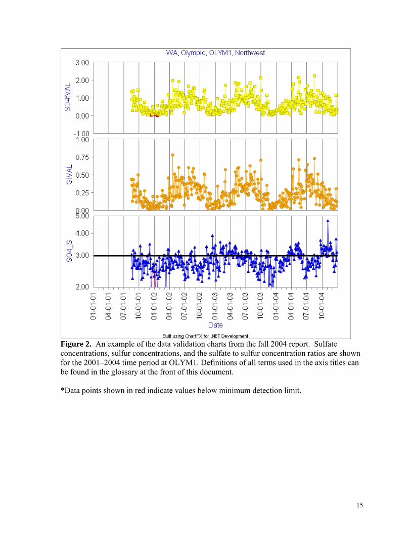
Figure 2. An example of the data validation charts from the fall 2004 report. Sulfate concentrations, sulfur concentrations, and the sulfate to sulfur concentration ratios are shown for the 2001–2004 time period at OLYM1. Definitions of all terms used in the axis titles can be found in the glossary at the front of this document.

*Data points shown in red indicate values below minimum detection limit.

15

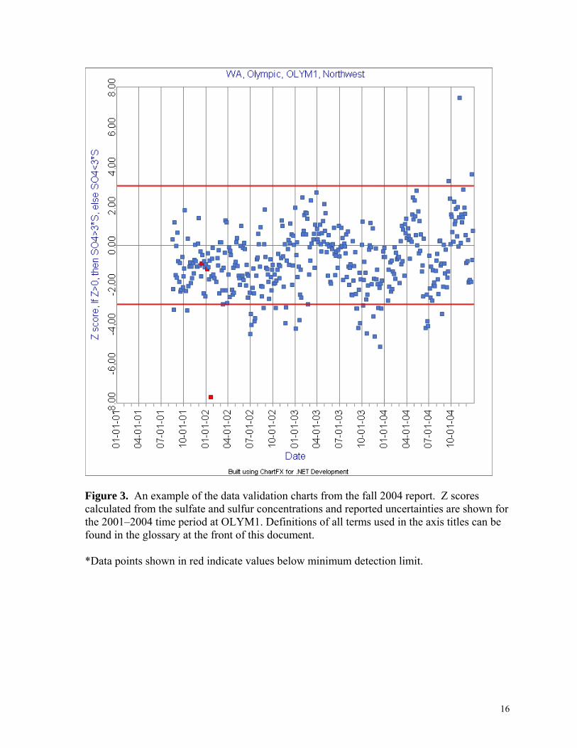
Figure 3. An example of the data validation charts from the fall 2004 report. Z scores calculated from the sulfate and sulfur concentrations and reported uncertainties are shown for the 2001–2004 time period at OLYM1. Definitions of all terms used in the axis titles can be found in the glossary at the front of this document. *Data points shown in red indicate values below minimum detection limit.

16

0.0

5.0

10.0

15.0

20.0

25.0

30.0

Jan-88

Jan-89

Jan-90

Jan-91

Jan-92

Jan-93

Jan-94

Jan-95

Jan-96

Jan-97

Jan-98

Jan-99

Jan-00

Jan-01

Jan-02

Jan-03

Jan-04

% outliers with SO4<<3*S % outliers with SO4>>3*S% outliers with SO4>>3*S or SO4<<3*S

Figure 4. The percentage of valid sample pairs with significant disagreement between SO4

= and 3*S are calculated for each month. This provides a way of tracking 1) the overall magnitude of the number of sample pairs with poor agreement relative to the number of samples collected as well as 2) the direction of bias at the network level. 4.2.3 Soil Elements With the exception of the collocated QC modules, there are no redundant measurements of the soil elements, so all validation efforts at this level focus on 1) internal consistency between the elements for a given sample and 2) consistency through time and, to a lesser extent space, for the elements individually and in relation to each other. Internal consistency between the soil elements is examined using soil enrichment factors (elemental ratio in aerosol/elemental ratio in average crustal rock), which roughly show if the soil elements in the aerosol sample are found in the same ratio as they would be in average crustal rock. Iron is the most stable element from the XRF systems, so it was selected as the reference element in calculating the enrichment factors. Individual samples are not examined for departures from the expected value of 1 for the enrichment factor; rather, the relative number of these samples and the typical value of the enrichment factor are monitored. Three panel time series charts are produced for each site for Al, Ca, Si, and Ti with the element of interest in the first, Fe in the second ,and the enrichment factor ((X/Feaerosol)/(X/Feaverage crustal rock)) for the element of interest in the third panel. The charts are examined primarily for changes in behavior in any of the three metrics over time that could indicate data quality problems.

%

17

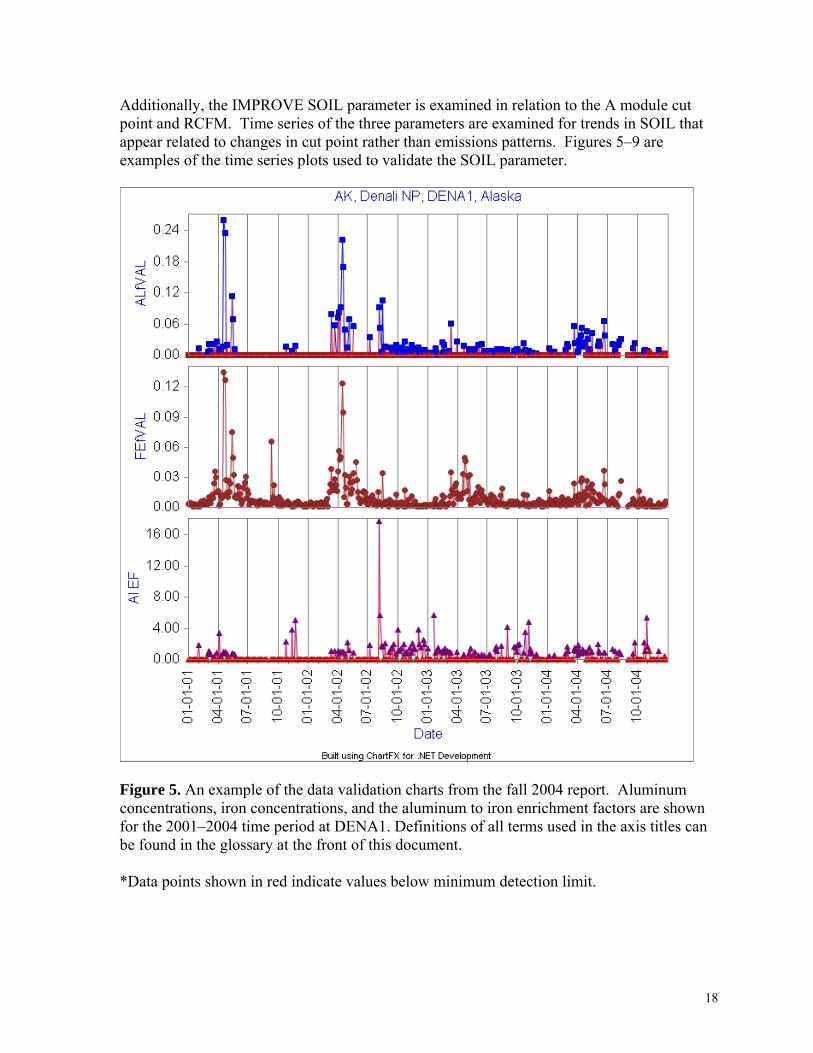
Additionally, the IMPROVE SOIL parameter is examined in relation to the A module cut point and RCFM. Time series of the three parameters are examined for trends in SOIL that appear related to changes in cut point rather than emissions patterns. Figures 5–9 are examples of the time series plots used to validate the SOIL parameter.

Figure 5. An example of the data validation charts from the fall 2004 report. Aluminum concentrations, iron concentrations, and the aluminum to iron enrichment factors are shown for the 2001–2004 time period at DENA1. Definitions of all terms used in the axis titles can be found in the glossary at the front of this document. *Data points shown in red indicate values below minimum detection limit.

18

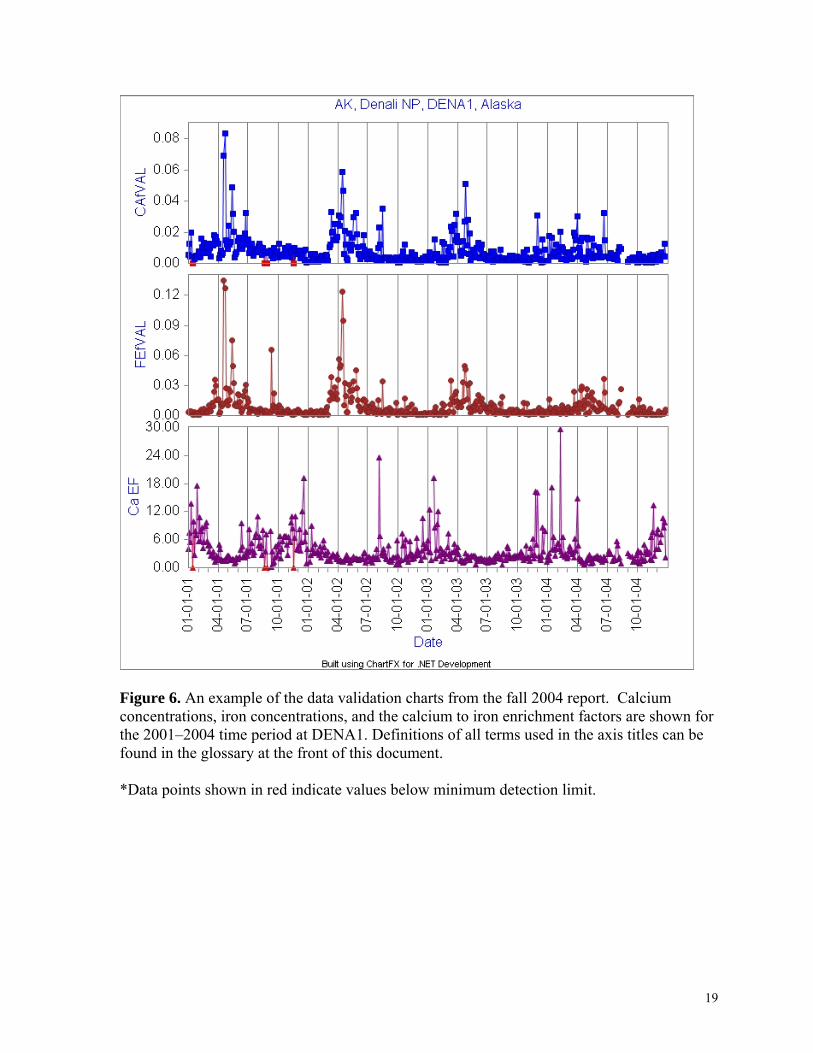
Figure 6. An example of the data validation charts from the fall 2004 report. Calcium concentrations, iron concentrations, and the calcium to iron enrichment factors are shown for the 2001–2004 time period at DENA1. Definitions of all terms used in the axis titles can be found in the glossary at the front of this document. *Data points shown in red indicate values below minimum detection limit.

19

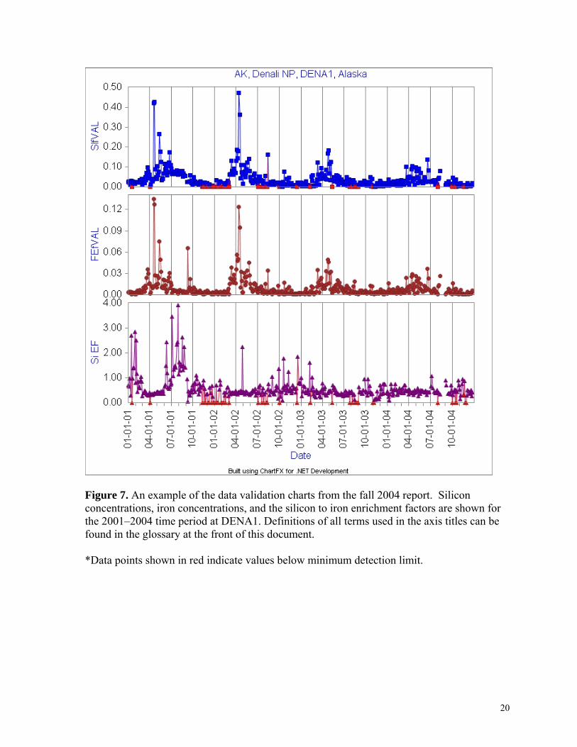
Figure 7. An example of the data validation charts from the fall 2004 report. Silicon concentrations, iron concentrations, and the silicon to iron enrichment factors are shown for the 2001–2004 time period at DENA1. Definitions of all terms used in the axis titles can be found in the glossary at the front of this document. *Data points shown in red indicate values below minimum detection limit.

20

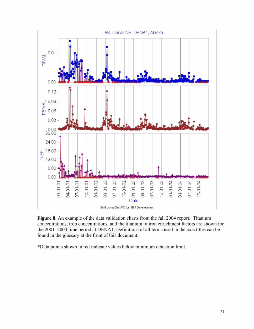
Figure 8. An example of the data validation charts from the fall 2004 report. Titanium concentrations, iron concentrations, and the titanium to iron enrichment factors are shown for the 2001–2004 time period at DENA1. Definitions of all terms used in the axis titles can be found in the glossary at the front of this document. *Data points shown in red indicate values below minimum detection limit.

21

Figure 9. An example of the data validation charts from the fall 2004 report. Soil concentrations, the A module cut point and the soil to reconstructed mass concentration ratios are shown for the 2001–2004 time period at DENA1. Definitions of all terms used in the axis titles can be found in the glossary at the front of this document. 4.2.4 Carbon In validating the carbon fractions OC and EC, the focus at this level is on analyzing time series of the data for abnormalities from 1) the general behavior at that site and 2) the general behavior observed at other sites. Spatial and seasonal variability in OC, EC, and the OC/EC ratio are expected given the varied sources and production pathways for carbonaceous aerosol. Figure 10 is an example of the time series of OC, EC, and OC/EC used for validating the carbon data.

22

The PESA hydrogen measurement can be used as an additional external validation of the OC measurement. OMH concentrations, an estimate of organic mass, are calculated from the hydrogen and sulfur concentrations by assuming that all sulfur is in the form of ammonium sulfate, no hydrogen is associated with nitrates or water, and the remaining hydrogen measured by PESA is from organic compounds. It is assumed that the volatile ammonium nitrate and water are quickly lost from the filter as soon as vacuum is applied to conduct the PESA analysis. Although OMH is merely an approximation of OMC, the two parameters should correlate well when the sampled aerosol is consistent with the assumption of sulfur being in the form of ammonium sulfate and all other measured hydrogen being associated with the carbon aerosol. Time series of OMC, OMH, and OMH/OMC are analyzed for abnormalities from the general behavior at that site and the general behavior observed at neighboring sites. Figure 11 is an example of the time series of OMC, OMH, and OMH/OMC used for validating the organic carbon data.

23

Figure 10. An example of the data validation charts from the fall 2004 report. Organic carbon concentrations, elemental carbon concentrations, and the organic carbon to elemental carbon concentration ratios are shown for the 2001–2004 time period at YOSE1. Definitions of all terms used in the axis titles can be found in the glossary at the front of this document.

24

Figure 11. An example of the data validation charts from the fall 2004 report. OMC concentrations, OMH concentrations, and the OMH to OMC concentration ratios are shown for the 2001–2004 time period at ACAD1. Definitions of all terms used in the axis titles can be found in the glossary at the front of this document. 4.2.5 Nitrate With the exception of the collocated QC modules, there are no redundant measurements of NO3

- so the validation efforts at this level are focused on analyzing time series of the data for abnormalities from 1) the general behavior at that site and 2) the general behavior observed at other sites. NO3

- is examined in relation to reconstructed fine mass (RCFM), allowing for analysis of changes in behavior in both the absolute and relative NO3

- concentrations. Figure 12 is an example of the time series used to validate NO3

-.

25

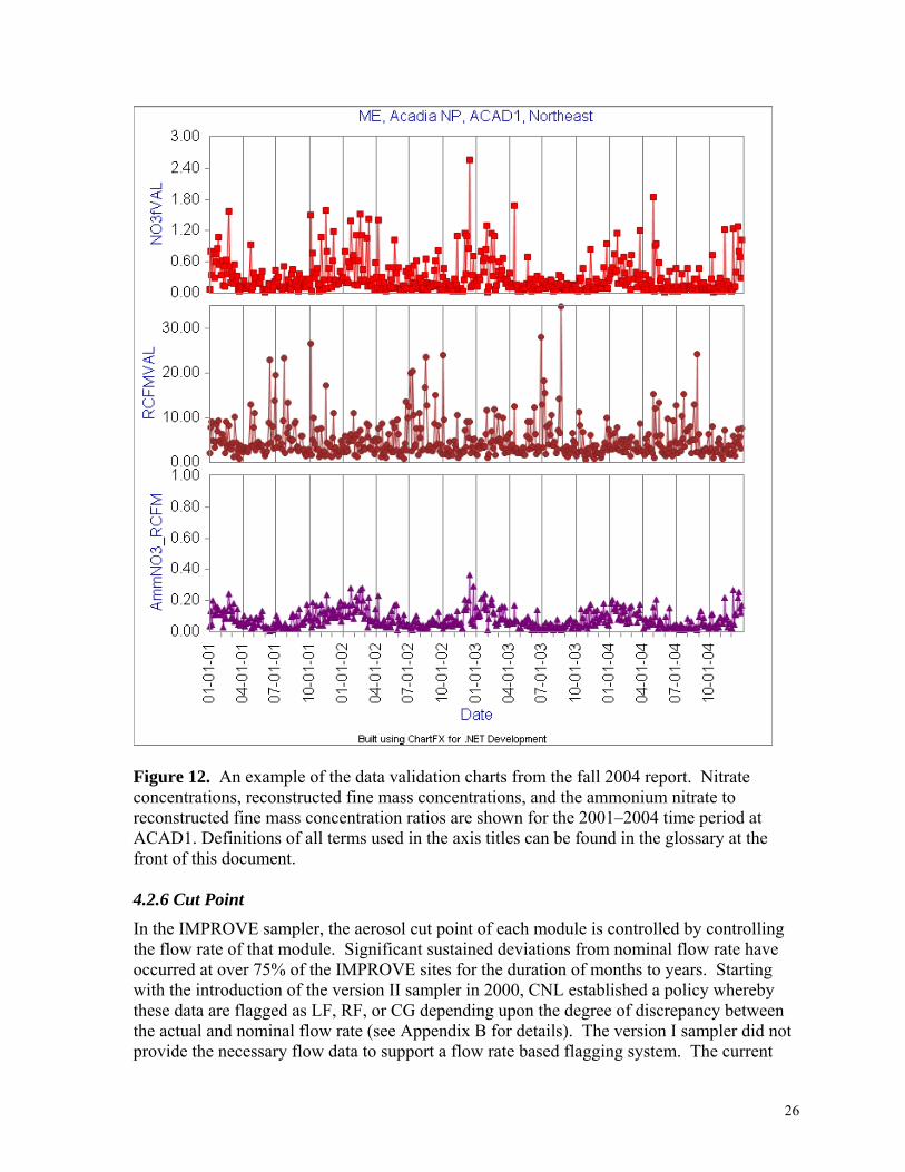
Figure 12. An example of the data validation charts from the fall 2004 report. Nitrate concentrations, reconstructed fine mass concentrations, and the ammonium nitrate to reconstructed fine mass concentration ratios are shown for the 2001–2004 time period at ACAD1. Definitions of all terms used in the axis titles can be found in the glossary at the front of this document. 4.2.6 Cut Point

In the IMPROVE sampler, the aerosol cut point of each module is controlled by controlling the flow rate of that module. Significant sustained deviations from nominal flow rate have occurred at over 75% of the IMPROVE sites for the duration of months to years. Starting with the introduction of the version II sampler in 2000, CNL established a policy whereby these data are flagged as LF, RF, or CG depending upon the degree of discrepancy between the actual and nominal flow rate (see Appendix B for details). The version I sampler did not provide the necessary flow data to support a flow rate based flagging system. The current

26

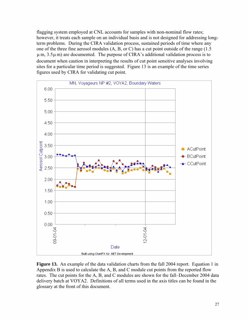
flagging system employed at CNL accounts for samples with non-nominal flow rates; however, it treats each sample on an individual basis and is not designed for addressing long-term problems. During the CIRA validation process, sustained periods of time where any one of the three fine aerosol modules (A, B, or C) has a cut point outside of the range (1.5

m, 3.5µm) are documented. The purpose of CIRA’s additional validation process is to document when caution in interpreting the results of cut point sensitive analyses involving sites for a particular time period is suggested. Figure 13 is an example of the time series figures used by CIRA for validating cut point.

µ

Figure 13. An example of the data validation charts from the fall 2004 report. Equation 1 in Appendix B is used to calculate the A, B, and C module cut points from the reported flow rates. The cut points for the A, B, and C modules are shown for the fall–December 2004 data delivery batch at VOYA2. Definitions of all terms used in the axis titles can be found in the glossary at the front of this document.

27

5. EXAMPLES OF DATA QUALITY ISSUES DISCOVERED BY CIRA IN THE 2004 DATA The primary outcome of the data validation procedures performed by CNL, DRI, and RTI is the qualified dataset delivered to CIRA. The QA personnel from these institutions assess the validity of the data on a data point by data point basis and apply validation flags to communicate the status of the individual data points to the user. The evolving flagging system is designed to communicate whether a data value is valid, questionable, or invalid, and, if the data is not valid, why. The types of problems identified and corrected through this process include misidentified filters, damaged samples, nonroutine sampling conditions, and nonroutine analysis conditions. Occasionally, the results of the data validation process point to inconclusive or questionable results and the need for reanalysis of either individual or batches of samples. In these cases the involved samples are, where possible, reanalyzed, and the data validation process starts over with the new results. Problems that are not resolved through reanalysis will result in data being identified and flagged as invalid. The data validation process at CIRA historically was part of data analysis studies and identified more subtle data quality problems that were difficult to detect with a single batch of data. The outcomes of these past checks have included small special studies, some still in progress, to understand data inconsistencies for identified issues as well as changes in data collection and data management practices and procedures. Examples of the special studies generated by these data validation efforts include

• Collocated sample collection with 25mm and 37mm nylon filters to determine if changes in face velocity affect the data,

• Testing of module B denuder coatings, and • Testing of alternate nylon filter extraction protocols.

Starting with the data collected during 2000, CIRA began a formal validation process that was expanded with the 2004 data and is now conducted for every data delivery during the 30-day preliminary data review period. The focus remains on identifying the more subtle data quality problems that affect large batches of data. The decisions of CNL, DRI, and RTI regarding the validity of individual data points are accepted and not examined outside of the context of data integrity checks. An example to illustrate the distinction is the quantitative validation checks on the comparability of SO4

= and S. The initial tests conducted at CNL are designed to identify temporally sequential sample pairs with significant disagreement that may indicate that the filters were swapped during the weighing process, whereas the tests at CIRA are designed to assess if the number of sample pairs in a batch of data that have significant disagreement between SO4

= and S is 1) statistically significant or 2) a change from past behavior for that site. Data quality problems identified during the first year of routine secondary data validation at CIRA have included identifying sampling problems, data processing errors, and data reporting errors. An additional goal of the process is the quantitative tracking of certain data quality metrics in order to assess trends and transitions in the overall quality of the

28

IMPROVE dataset. The special studies resulting more recently from CIRA’s validation efforts include

• Testing of clogged inlets, • Fully characterizing the cyclone and the effect of changing flow rate on cut point, • Fully characterizing the XRF systems.

Data reporting errors have included the unintentional inclusion of internal validation flags in the data deliveries, the incorrect use or mapping of validation flags, and the incorrect file format. All of the identified data reporting problems were resolved through data resubmissions, usually within the 30-day review period. Some of the data processing errors were more complicated and have resulted in broader solutions. One such error identified in the fall 2004 data was erroneously calculated flow rates in the cases where the nominal flow readings were used to calculate the flow rate. The error was identified during the visual inspection of the cut points for each site as an anomalous drop in cut point in all three modules in a handful of data records (Figure 14). The anomaly was reported to CNL and their review found an error in how the flows were calculated. The error was introduced to the CNL data management system when the code for calculating the flow rates was rewritten to accommodate an updated operating system. The flow rate calculation program was corrected and the fall 2004 data were redelivered.

29

Figure 14. An example of the flow rate problem discovered in the data validation charts from the fall 2004 report. Equation 1 in Appendix B is used to calculate the A, B, and C module cut points from the reported flow rates. The cut points for the A, B, and C modules are shown for the fall–December 2004 data delivery batch at HOOV1. Definitions of all terms used in the axis titles can be found in the glossary at the front of this document. The routine data integrity checks also lead to the discovery of undocumented changes to the delivery files. Further communication with the QA personnel at CNL confirmed that the CNL data management system lacks write protections and change tracking. In response to these findings, CNL has accelerated their efforts to thoroughly update and redesign their data management system. Unlike the data reporting and data processing errors that were primarily found through automated data integrity tests, the sampling problems were identified through CIRA’s

30

exploratory data validation process. The most significant discovery in 2004 was an inlet clogging problem associated with a particular inlet design that was difficult to clean. The clogging resulted in incomplete sample collection for the affected module at Chassahowitzka NWR (CHAS1), Mingo (MING1), and Swanquarter (SWAN1) for several years. This problem was identifiable at CHAS1 and SWAN1 through on-going degradation in the internal consistency tests (Figure 15, a and b) and at MING1 through a decreasing trend in the organic and elemental carbon that was not present at neighboring sites (not displayed). The combination of two factors related to the CNL data validation system allowed this sampling problem to remain undetected for 1–2 years at three sites. The first factor was that their validation system does not allow the evaluation of data in context of past behavior, and the second was the assumption that poor comparability between associated samples is due to uncontrollable random errors unless a known problem can be identified. Once the problem was identified, CNL took several key steps to address the underlying problem. All sites that showed any internal consistency problems and that had the same inlet design as at the identified three sites had new inlets of a more easily maintained design installed. These sites had new inlets mailed to them and the site operators were instructed as to how to install the new inlets. During the 2005 and 2006 field seasons, the remaining sites with the problematic inlets will have new inlets installed during their annual maintenance visit. As part of this effort the field technicians were retrained on the importance of cleaning the inlets as part of the annual site maintenance. The clogged inlets from CHAS1, SWAN1, and MING1, along with those removed from unaffected or less affected sites, were used to study the impacts of inlet clogging on sample collection. The results of these studies indicated that the inlet needed to be almost completely clogged before it had noticeable impacts on sample collection. The analysis of S/SO4

=, OMH/OMC and LRNC/LAC ratios was also added to the CNL data validation process.

31

a)

0

1000

2000

3000

4000

5000

6000

7000

8000

6/2 6/14 6/26 7/8 7/20 8/1 8/13 8/25

Σ S3 Σ SO4r

Con

cent

ratio

n (n

g/m

3 )

32

b)

Figure 15, a and b. An example of the data validation charts from CNL (a) and from CIRA’s summer 2004 report (b). Panel a shows sulfate and three times sulfur concentrations for summer 2004 at CHAS1. Panel b shows sulfate concentrations, sulfur concentrations, and the sulfate to sulfur concentration ratios for 2001–2004 at CHAS1. While the incomplete sampling on the A module is obvious in panel b, the sulfate to sulfur discrepancies in panel a do not look similarly alarming. The sampling problem, which is obvious starting in early 2003, was not caught until the 2004 data were examined at CIRA and was not fully acted upon until the summer of 2004. Definitions of all terms used in the axis titles can be found in the glossary at the front of this document.

Period shown on other graph

33

6. REFERENCES: Crocker Nuclear Laboratory, SOP 251 Sample Handling,

http://vista.cira.colostate.edu/improve/Publications/SOPs/ucdavis_sops/sop251.pdf Crocker Nuclear Laboratory, SOP 301 X-Ray Fluorescence Analysis,

http://vista.cira.colostate.edu/improve/Publications/SOPs/ucdavis_sops/sop301.pdf Crocker Nuclear Laboratory, SOP 326 PIXE and PESA Analysis,

http://vista.cira.colostate.edu/improve/Publications/SOPs/ucdavis_sops/sop326.pdf Chow, J.C., J.G. Watson, L.C. Pritchett, W.R. Pierson, C.A. Frazier, and R.G. Purcell, The DRI

thermal/optical reflectance carbon analysis system: description, evaluation, and applications in U.S. air quality studies, Atmos. Environ., 27(A), (8), 1185-1201, 1993.

Chow et al., Comparison of the DRI/OGC and Model 2001 Thermal/Optical Carbon

Analyzers, 2005 Clark, M.S., Performance Evaluation—IMPROVE Laboratories, Technical Memorandum,

2003 Desert Research Institute, IMPROVE Standard Operating Protocols Carbon Analysis,

http://vista.cira.colostate.edu/improve/Publications/SOPs/drisop.asp Dyson, A., L.L. Ashbaugh, Characterization of Nylon Filters used in the IMPROVE

Network, Regional and Global Perspectives on Haze: Causes, Consequences and Controversies Visibility Specialty Conference, Asheville, NC, A&WMA, October 2004.

EPA, EPA Quality Manual for Environmental Programs, Office of Environmental

Information Quality Staff, Washington D.C., 2000. EPA, Guidance for Tracking Progress Under the Regional Haze Rule, Office of Air Quality

Planning and Standards, Research Triangle Park, NC, 2003 McDade, C., Summary of IMPROVE Nitrate Measurements, internal report, 2004. McDade, C.E., R. A. Eldred, and L. L. Ashbaugh, Artifact Corrections in IMPROVE,

Regional and Global Perspectives on Haze: Causes, Consequences and Controversies Visibility Specialty Conference, Asheville, NC, A&WMA, October 2004.

Research Triangle Institute, “Standard Operating Procedures for National Park Service Filter

Preparation, Extraction, And Anion Analysis”, http://vista.cira.colostate.edu/improve/Publications/SOPs/RTI_SOPs/RTI_IonSOP.pdf

Rice, J.A., Mathematical Statistics and Data Analysis, Duxbury Press, Belmont, CA, 1995.

34

Yu, X., T. Lee, B. Ayres, S. M. Kreidenweis, W. C. Malm and J.L. Collett, Jr., “Particulate Nitrate Measurement Using Nylon Filters”, in press in JAWMA 2005.

35

Appendix A. Data Acquisition, Quality Control, and Data Management The standard IMPROVE sampler has four independent sampling modules: A, B, and C collect PM2.5 particles (0–2.5 µm), and D collects PM10 particles (0–10 um). Module A utilizes a Teflon filter that is analyzed for gravimetric mass and elemental concentrations by X-ray fluorescence (XRF) and proton elastic scattering analysis (PESA) and prior to 12/2001 by proton induced X-ray emission (PIXE). Module B utilizes a nylon filter and is analyzed primarily for anions by ion chromatography (IC). Module C utilizes a quartz filter and is analyzed for organic and elemental carbon by TOR carbon analysis (TOR). Module D utilizes a Teflon filter and is analyzed for gravimetric mass. Sample Handling Samples are processed on a monthly basis. Separate files are kept for field logs, results from each analysis procedure (weights, laser absorption, XRF, IC, and carbon), comments, flow rates, and sampler calibrations. Each module and filter cassette is color-coded and designated by a letter. Custom software tracks each sample by site, sample date, and start time. Each sample’s intended sampling date and location is assigned by the computer. Additionally, the computer also assigns when field blanks or after-filters should be included in the shipment. Samples can be pre-weighed or post-weighed on any one of four balances; they are all calibrated and cross-checked twice daily to ensure consistency. Laboratory blanks are weighed on each balance twice each day, then are loaded into cassettes, stored on a shelf for six weeks, and weighed again. When sample shipments are received for processing, the log sheets are checked and the flow, elapsed time, and temperature are downloaded from a flash memory card that stores the electronic data from the sampler. The sample boxes are then sorted alphabetically for all subsequent processing. At this point the computer knows the sample box has been received (by site and sample date) and prompts the sample-handling technician through all the sample handling steps. The nylon and quartz filters are removed from cassettes and placed into Petri dishes for shipping to the appropriate analysis contractor. Filter labels are transferred to the Petri dishes from the cassette holder as the filters are unloaded. The computer records their position in the queue of samples. The Teflon filters are post-weighed, and the net weight is immediately calculated to confirm that the difference is positive. The PM10 net weights are also compared to the PM2.5 net weights to ensure that the PM10 mass is greater than the PM2.5 mass. Whenever a discrepancy is found, the weighing technician must call a supervisor before continuing. After being post-weighed, the PM2.5 and PM10 Teflon filters are mounted into slides and the slides are filed into slide trays. The PM2.5 slide trays are delivered to the XRF lab for analysis. The gravimetric analysis of both the A and D module Teflon filters allows for the estimation of the coarse aerosol fraction by subtracting the PM2.5 mass from the PM10 mass. After all the used samples are processed, the empty box is sent to the pre-weight station to be prepared for the next round of samples. The software prompts the technician to weigh the correct filters for the box, and prints filter labels and log sheets to go with them. Sample boxes are checked and rechecked several times before being shipped to sites.

36

Sample Analysis The PM2.5 Teflon filters are analyzed for elemental content by CNL. The forms of elemental analysis conducted past and present in the IMPROVE network are PESA, PIXE, and XRF. PESA has been and continues to be used for quantifying elemental hydrogen. PIXE was initially used for quantifying all other elements reported—nearly all elements with atomic number ≥11 (which is Na) and ≤82 (which is Pb). Beginning in 1992 analysis of the heavier elements, those with atomic weights from Fe to Pb, was changed from PIXE to XRF with a Mo anode source. PIXE was discontinued in late 2001 and analysis of the lighter elements with atomic numbers from Na to Mn was changed from PIXE to XRF with a Cu anode source. Additionally, the Fe measurements from the Cu XRF system were reported to the final database instead of those from the Mo system. In both cases the change from PIXE to XRF provided lower minimum detection limits for particular elements of interest, as well as better sample preservation for reanalysis. Under current procedures, XRF runs are carried out in 1-month sample batches (e.g., all samples collected in March). Once each month on the Mo system, and once each week on the Cu system, a set of standard foils is run. The Cu system is more subject to change due to the helium atmosphere it runs in and is therefore checked more frequently. The standard foils serve two purposes: 1) to obtain the relationship between X-ray energy and the multi-channel analyzer bin number that the X-rays are counted in and 2) to check the overall calculation against the standard amount. For elements with atomic weights ≥Si, the values reported fore each foil must agree with the known amount within 5% or the analysis is aborted until the reason is found. Several of the standards are more heavily loaded than routine sample filters and must be run at a lower X-ray tube current. After establishing that the standards are measured correctly, a designated set of previously analyzed samples is run at the normal operating current. These samples have been analyzed multiple times as a check of the system against drift. They contain a range of values typical of those in the network and serve a similar function to a multipoint calibration. The reanalysis samples are checked against the prior known values by a separate regression for each element. The Cu system is checked using a set of low atomic number elements that includes S, Ca, Ti, Fe, and others, and the Mo system is checked using a set of higher atomic number elements appropriate to that system. If any of the regression slopes differ by more than 5%, the run is stopped and the reason is found and corrected. Problems with the replicate analysis are rarely seen once the standards are checked and approved. The regression analysis is more appropriate for the reanalysis samples than a point-by-point test, because statistical counting uncertainties can affect any individual point. The nylon filters are analyzed by RTI using IC for the major anions Cl-, NO3

- and SO4=, with

the primary parameter of interest being the NO3-. Multipoint calibrations and QA/QC

standards are run daily prior to any samples. Analysis of samples does not proceed unless the observed values for SO4

= differ by less than 10% from the known values. The IMPROVE quartz filters are analyzed by DRI for organic and elemental carbon using TOR. IMPROVE has used the same thermal optical reflectance protocol since 1988 for measuring organic carbon (OC) and elemental carbon (EC) fractions of total carbonaceous

37

aerosol. Fractionation of the aerosol is controlled and defined by changes in the analysis temperature and atmosphere and changes in filter reflectance. The OC fractions are evolved first in an inert, ultrahigh purity helium environment, O2 is then introduced to the sampling chamber to evolve the EC fractions. Evolved carbon for each fraction is quantified using a flame ionization detector (FID) gas chromatograph (GC). The GC is calibrated daily using National Institute of Standards and Technology (NIST) traceable CH4 and CO2 calibration gases. In addition, semi-annually the calibration slopes derived from the two gases and the potassium hydrogen phthalate (KHP) and sucrose-spiked filter punches are averaged together to yield a single calibration slope for a given analyzer. This slope represents the response of the entire carbon analyzer to generic carbon compounds and includes the efficiencies of the oxidation and methanator zones and the sensitivity of the FID. Note that the current calibration procedure is based only on the total carbon; currently no routine procedure exists to check the accuracy of the OC/EC split. Comparability between aerosol carbon measurements, particularly the fractions, is highly dependent on measurement protocol. Recent analysis of the DRI/Oregon Graduate Center (OGC) analyzers used for IMPROVE carbon analysis since 1987 revealed that certain variables were not controlled as well as previously thought in these instruments. The possibility exists that poorly controlled aspects of the instrumentation may have caused changes in the OC/EC ratio over time. A small leak in the instrument allowed the diffusion of ambient air into the sampling chamber; the level of oxygen contamination in the helium atmosphere could have changed over time, affecting the stability of the OC/EC ratio. Furthermore, the OC/EC ratio can also be impacted for individual samples by the presence of oxidizing minerals or catalysts (such as NaCl), further complicating the situation. However, total carbon (TC), OC, and EC seemed to be reproducible within measurement uncertainty for filters back to 1999. The Model 2001 carbon analyzer includes an updated protocol and is slated for implementation starting with samples collected in 2005. The IMPROVE system has been designed to include internal measurement redundancy, a valuable asset for data validation. Examples include Fe from both XRF systems, SO4

= and S from modules B and A, respectively, and various modeled relationships that allow for the intercomparison of results from the independent modules (see section 2.5.2 for more detail). When all samples for a month have been analyzed and the datasets are complete, they are combined by custom software into a single data table that is then reviewed site-by-site for internal consistency.

38

Appendix B. Data Validation Activities at CNL B.1 Flow Rate Audits and Analysis Performed by CNL Flow rate accuracy is a critical aspect of overall system accuracy. The A, B, and C modules of the IMPROVE sampler are intended to sample fine aerosol with a cut point of 2.5 µm. The cut points of the modules are controlled by the flow rate for that module. Based on the design of the sampler, flow rate is inversely related to cut point as shown in Figure 1 and modeled in equation 1: ( )75.22*334.05.250 −−= Qd (1) where Q = flow rate (L/min) and d50 = aerodynamic diameter at which 50% of the particles are collected (µm). Equation 1 was developed based on flow rates between 18 and 24 L/min. Beyond these flow rates, equation 1 may not be valid.

2.0

2.5

3.0

3.5

4.0

4.5

18 20 22 24

flow rate (L/min)

d(ae

) for

50%

effi

cien

cy

PSLSPART

Figure 1. The plot shows the 50% cut point as a function of flow rate as determined by two separate collection efficiency tests. The collection efficiency of the IMPROVE cyclone was characterized at the Health Sciences Instrumentation Facility at the University of California at Davis. The efficiency was measured as a function of particle size and flow rate using two separate methods: PSL and SPART. The PSL method uses microspheres of fluorescent polystyrene latex particles (PSL) produced by a Lovelace nebulizer and a vibrating stream generator and analyzed by electron micrographs. The SPART method uses a mixture of PSL particles produced by a Lovelace nebulizer and analyzed by a Single Particle Aerodynamic Relaxation Time (SPART) analyzer. The aerodynamic diameter for 50% collection, d50, was determined for each flow rate.

39

Efforts are made to maintain the flow rate at a nominal rate of 22.8 L/min in order to achieve the desired cut point. These efforts include annual calibrations of the sampler as well as periodic internal and external flow rate audits to test if the system is within tolerable limits for meeting the MQOs. Corrective action is taken if an audit indicates problems. However, there are a variety of reasons why the average flow rate of a given 24-hour sample may vary from the nominal rate from clogging due to heavy aerosol loading on the filter to equipment failure. A flagging system is in place to qualify samples with severe deviations from the nominal flow rate and therefore from a cut point of 2.5 µm (Table 1). However, only those samples flagged as clogged filter (CL) are considered invalid, thus allowing even those samples that would have estimated cut points outside of the range 1–4 µm (assuming linearity outside of the documented range of equation 1) to be considered qualified valid samples. Currently all flow related validation criteria are based only on individual samples; there are no population level checks on how many samples can be flagged as low/high flow rate (LF) or really high flow rate (RF). Table 2. Flow rate-related validation flag definitions and application criteria. Validation Flag

Definition Concentration Reported?

Criteria

CL Clogged Filter

No Flowrate less than 15 L/min for more than 1 hour

CG Clogging Filter

Yes Flowrate less than 18 L/min for more than 1 hour 1

LF Low/high flow rate

Yes Average flowrate results in cutpoint outside 2-3 µm (corresponds to flowrates < 21.3 L/min or > 24.3 L/min).

RF Really low/high flow rate

Yes Flow greater than 27 L/min for more than 1 hour 2

B.2 Accuracy, Uncertainty, and MQL Checks on QC Samples Performed at CNL A positive feature of the IMPROVE dataset is the calculation and reporting of uncertainty and minimum detection limit (MDL) for every data point. The uncertainty estimate is useful for quantitative comparisons of similar data such as the collocated data and SO4

= and S. The MDL is useful for evaluating the robustness of the measured values. The uncertainty and MDL calculations are in part based on the results of select QC tests. All calibration standards for XRF, IC, and TOR are NIST traceable. Calibrations are performed prior to analyzing every batch of samples. Adjustments are made to the systems until they are in agreement with the known standards within a tolerable range for meeting the MQOs for accuracy. Replicate samples are run as part of every batch to ensure that the system’s precision remains within tolerable limits for meeting the MQOs. A further test on the precision of the overall sampling and analytical system is collocated samplers. The observed differences in collocated data are directly comparable to the MQOs. Also, the observed differences in

40

collocated data are compared to the estimated uncertainties reported with each data value to determine if the reported values are accurate. New data validation tests to ensure MQO conformance will likely be developed as part of the MQO review and revision process. B.3 Internal Consistency Checks Performed at CNL B.3.1 Iron Both X-ray systems are equally sensitive for iron, and comparisons of the iron measurements from the two systems are a routine part of CNL’s QA system. A scatter plot of iron from the Cu and Mo XRF systems is examined for every data batch. Valid data are expected to have a correlation slope of 1±0.05. B.3.2 Mass Given accurate cut points on both the A and D modules, valid sample sets are expected to have PM10 masses that are equivalent to or greater than PM2.5 masses. Therefore, every sample in the batch is analyzed to see if PM10-PM2.5≥0, within measurement uncertainty, both at the time of weighing and after all modules have been analyzed. Cases where PM10-PM2.5≤0 are evaluated for potential filter swaps. Additionally, the reconstructed fine mass (RCFM) from the speciated concentrations and the measured fine (MF) mass are expected to be roughly equivalent for a sample set. Every sample in the batch is analyzed to see if RCFM and MF agree within subjective expectations after all modules have been analyzed. The qualitative analysis is based on the visual inspection of time series figures by the QA manager. Large discrepancies between reconstructed and measured fine mass can indicate data quality problems in any one or a subset of the measurements involved in the comparison. B.3.3 Sulfate A quality assurance check for the A and B modules consists of comparison of the measured concentrations of sulfur and sulfate. The comparison also provides an external check on the IC and XRF systems. Since both modules should be sampling simultaneously and have the same flow and aerosol size cut point and assuming all aerosol sulfur is in the form of sulfate the collected data should be equivalent. Every sample in the batch is analyzed to see if SO4

= and 3*S agree within subjective expectations after all modules have been analyzed. The qualitative analysis is based on the visual inspection of time series figures by the QA manager. Additionally, a quantitative check on the agreement of the two measurements is used to evaluate temporally consecutive sample pairs for potential filter swaps. B.3.4 Carbon A correlation plot of the concentration of organic mass from hydrogen analysis (OMH) and the concentration of organic mass from carbon analysis (OMC) is examined as an external validation check on the carbon measurements from the C module. OMH concentrations are determined by assuming that all sulfur is in the form of ammonium sulfate, no hydrogen is associated with nitrates or water, and the remaining hydrogen measured by PESA is from organic compounds. It is assumed that the volatile ammonium nitrate and water are quickly

41

lost from the filter as soon as vacuum is applied to conduct the PESA analysis. OMC concentrations are derived through TOR analysis. Although OMH is merely an approximation of OMC, the two parameters should correlate well under certain sampling conditions. The dataset is analyzed to see if OMH is in agreement with OMC within subjective expectations after all modules have been analyzed. The analysis is qualitative and based on the judgment of the QA manager.

42