origin-based algorithms for traffic assignment: algorithmic structure, complexity...

ORIGIN-BASED ALGORITHMS FOR TRAFFIC ASSIGNMENT: ALGORITHMIC

STRUCTURE, COMPLEXITY ANALYSIS, AND CONVERGENCE PERFORMANCE

Jun Xie, Ph.D.

Postdoctoral Researcher

School of Naval Architecture, Ocean and Civil Engineering

Shanghai Jiaotong University

800 Dongchuan Rd.

Shanghai 200240, China

Phone: +86 (21) 3420-6196

Fax: +86 (21) 3420-6197

Email: [email protected]

Chi Xie, Ph.D.

Professor

School of Naval Architecture, Ocean and Civil Engineering

Shanghai Jiaotong University

800 Dongchuan Rd.

Shanghai 200240, China

Phone: +86 (21) 3420-8385

Fax: +86 (21) 3420-6197

Email: [email protected].

Text: 5,970 words

Figures and tables: 6

Total length: 7,470 words

Submitted for presentation at the 94th Transportation Research Board Annual Meeting, January

11-15, 2015, Washington, D.C. and publication in the Transportation Research Record

J. Xie and C. Xie 1

ABSTRACT 1

This paper presents an extensive analytical and numerical investigation on a class of origin-based 2

algorithms for the user equilibrium-based traffic assignment problem. A total of nine known 3

algorithms in this class are first clustered into four algorithmic structures, based on their 4

structural differences and similarities in algorithm design. We further conduct a complexity 5

analysis on these different algorithmic structures by calculating the frequency of executing node 6

and link operations, which provides a simple analytical way to estimate their per-iteration 7

computational costs. To deliver a comprehensive and fair comparison on their convergence 8

performance, all these nine algorithms are then implemented on the same programming platform 9

and run to solve a few representative large-scale traffic networks with different sizes and 10

congestion levels. A close look on the convergence performance statistics further justifies the 11

consistency of the complexity analysis and numerical evaluation results on the computational 12

efficiency of these algorithms. Discussions on the degeneration of algorithm convergence 13

efficiency with respect to network size and congestion level provide useful insights for the 14

potential improvement of current origin-based algorithms or the proposition of new algorithms. 15

Keywords: traffic assignment; user equilibrium; origin-based algorithms; bushes; paired 16

alternative segments; complexity analysis; convergence performance17

J. Xie and C. Xie 2

INTRODUCTION 1

Traffic assignment has been widely used as the standard tool to predict network flow patterns in 2

the final stage of travel demand forecasting. Although various traffic assignment models that can 3

capture more realistic features of real traffic systems have been explored and studied, such as 4

dynamic traffic assignment (1, 2) and stochastic traffic assignment models (3, 4), we see that the 5

most frequently used traffic assignment model in practice is still the static deterministic model 6

under the user equilibrium (UE) principle, which states that for every origin-destination (O-D) 7

pair all used routes have equal travel costs and no unused route has a lower cost (5). Several 8

superiorities of the UE model is easy to enumerate, including its intuitive assumptions, simple 9

formulations and stable solutions with respect to inputs. To our knowledge, the most important 10

advantage of the UE model in comparison to other models may attribute to its various kinds of 11

solution methods that can solve large-scale network problems efficiently. 12

The first class of practical TAP algorithms operates in the space of link flows, known as link-13

based algorithms, such as the Frank-Wolfe (FW) algorithm and its variants (6-8). Easy 14

implementation and fast convergence in early iterations allow these algorithms to emerge as the 15

winner in the transportation planning practice over the past decades. However, the main 16

shortcoming of the link-based algorithms is their inability to obtain high-precision solutions in 17

most practical applications. To address this issue, path-based algorithms, which generate, store 18

and equilibrate a relative small number of paths for each O-D pairs, have been considered in the 19

literature(9-11). In general, path-based algorithms work well for small- and medium-size 20

problems, yet their efficiency degrade significantly with the problem size increasing (12). 21

This paper studies and compares a class of origin-based algorithms for the traffic assignment 22

problem (TAP), which promise to produce highly precise UE solutions. All algorithms involved 23

in this paper are characterized by the “origin-based” feature, by which TAP is decomposed into a 24

sequence of subproblems with respect to origins; each one can be solved to an origin-based UE 25

solution representation restricted on a single-origin network, and then loops among all origins to 26

equilibrate the entire network. Under the above relatively relaxed definition, a number of 27

algorithms can be classified into this family, most of which were developed in the past decade. 28

The best known algorithm of this class is the Origin-Based Algorithm (OBA) developed by Bar-29

Gera (13). Nie (14, 15) revised Bar-Gera’s OBA by fixing an error in computing the second-30

order derivative, and circumventing the line search in solving the restricted master problem 31

(RMP) defined on each bush rooted at the origin. In this paper, we call Nie’s revised algorithm 32

QBA following his original paper. Gentile (16) proposed to use the greedy method to solve the 33

sequence of approximated quadratic programs, and named the resulting algorithm the Local User 34

Cost Equilibrium (LUCE) algorithm. Dial (17) proposed the so-called Algorithm B by solving 35

the RMP directly by swapping flows from the longest path to the shortest path for each node on 36

the bush, taking advantage of the acyclicity of a bush. Zheng and Peeta (18) proposed a variant 37

J. Xie and C. Xie 3

of Algorithm B by successively refining an endogenously determined 𝜀 value to solve the RMP 1

into 𝜀-optimal flows. The above five algorithms all recognize the fact that links with positive 2

flows under UE will never form a directed cycle, and choose to maintain a bush for each origin 3

and operate flows on bush links only. In this regard, these algorithms are also referred to as bush-4

based algorithms. 5

Another highly efficient algorithmic structure widely used in the design of origin-based 6

algorithms is paired alternative segments (PAS). The concept of PAS was recently proposed by 7

Bar-Gera (19), though the use of it for TAP actually has a much longer history. To our best 8

knowledge, the Network Simplex (NS) method adapted by Nguyen (20) was the first algorithm 9

that identifies and uses PASs for TAP. It maintains a spanning tree for each origin such that a 10

PAS can be detected by augmenting an out-of-tree link into the tree. This idea is recently 11

revisited by Zheng (21), who fixed a pivot rule error of NS and proposed a generalization of this 12

algorithm by allowing the spanning tree to contain links that could either emanate from or point 13

toward the origin. For discussion convenience, this revised NS algorithm is abbreviated as RNS 14

in this paper. His numerical results testified the high efficiency of using PASs in solving large-15

size problems. It is somewhat surprising that the NS algorithm has not received much attention, 16

though it has great potential to achieve high performance and it was applied for TAP earlier than 17

the FW algorithm. Another algorithm that uses PASs is Dial’s Algorithm B (17), in which a bush 18

is preserved for each origin instead. Thanks to the acyclicity of a bush, a PAS can be identified 19

by following the shortest and longest path segments ending at the same node. Use of PASs for 20

TAP was more systematically explored by Bar-Gera in developing his famous TAPAS algorithm 21

(19), where a breadth first search method that can directly identify PASs from the shortest path 22

tree rooted at each origin is applied. Xie and Xie recently (22) improved TAPAS by proposing a 23

new PAS identification method that continuously identifies the higher cost segment with the 24

maximum flow link in the backward set of the nodes and relates only one origin to each PAS. 25

Their numerical experiments show that the improved TAPAS (termed iTAPAS) can be two 26

times faster than TAPAS in solving large networks. The above five algorithms all identify and 27

operate PASs for a TAP formulated at one origin. Hence we can call them PAS-based algorithms. 28

Note that Algorithm B can be categorized into both the bush-based and PAS-based algorithms as 29

it uses bushes and PASs simultaneously. 30

In this paper, our main research purpose is to make a fair and systematic comparison on the class 31

of origin-based algorithms. To this end, we investigated all known origin-based algorithms and 32

their variants and compared them in the following two aspects. First, we provided four 33

algorithmic structures to accommodate the nine algorithms of interest. For algorithms that utilize 34

the same structure, we compare them by examining their similarities and differences in 35

algorithmic details. For algorithms that belong to different structures, we try to make a 36

comparison on their computation costs of each iteration by estimating the frequency of scanning 37

the set of nodes and links for each structure. (Hereafter in this paper, such an evaluation of the 38

computation costs pertaining to these different algorithmic structures is termed structural 39

J. Xie and C. Xie 4

complexity in this paper, which is different from the widely used definition of computational 1

complexity. The latter typically takes into account very basic algorithmic operations, such as 2

assignment, arithmetic and logical operations, in the worst case of problem instances.) Second, 3

we implemented all nine algorithms on the same programming platform and let different 4

algorithms share as many subroutines as possible. Extensive numerical experiments were 5

conducted on both medium- and large-scale test problems to provide an overall comparison in 6

terms of convergence efficiency. Several per-iteration convergence statistics are examined as 7

well to provide insights and explanations for the convergence behavior of different algorithms. 8

Extensive and systematic comparisons of the latest UE algorithms are important and essential to 9

transportation planning practitioners and software developers, since they need to know which 10

algorithms will satisfy their needs. We note that Inoue and Maruyama (12) conducted a very 11

good comparison on the traditional link-based, path-based, and some of origin-based algorithms. 12

We advance their work by adding several new algorithms and place our focus only on the class 13

of state-of-the-art origin-based algorithms. We also contribute the literature through this paper by 14

estimating the structural complexity of these algorithms, which provides an analytical way to 15

assess and compare the computation costs of the algorithms. 16

The rest of this paper is organized as follows. Section 2 describes the notation and algorithmic 17

terms that are used in this paper. In Section 3, we briefly review and compare the nine algorithms 18

considered in this paper by categorizing them into four algorithmic structures and estimating 19

their structural complexity. The convergence performance of the nine algorithms are then 20

compared and analyzed in Section 4. The last section concludes the paper with a few remarks on 21

the major findings and future research. 22

NOTATION AND ALGORITHMIC TERMS 23

Consider a directed traffic network 𝐺(𝑁, 𝐴) where 𝑁 and 𝐴 denote the sets of nodes and links, 24

respectively. Suppose 𝐺 is strongly connected, by which we mean that there is at least one path 25

connecting any two nodes in 𝐺. 𝑁 consists of a set of nodes, some of which are origins denoted 26

by 𝑅 and some others of which are destinations denoted by 𝑆. The travel demand departing from 27

an origin 𝑟 ∈ 𝑅 to an destinations 𝑠 ∈ 𝑆 is denoted by 𝑑𝑟𝑠. Link (𝑖, 𝑗) is directed from node 𝑖 to 28

node 𝑗. Let 𝑥𝑖𝑗 be the traffic flow on link (𝑖, 𝑗) ∈ 𝐴 and 𝑡𝑖𝑗(∙) be the travel time of traversing link 29

(𝑖, 𝑗), which is a strictly positive, increasing and convex function of 𝑥𝑖𝑗. 30

Given the above network, the UE-based TAP can be formulated as a convex optimization 31

problem with linear constraints. Existing algorithms usually decompose a TAP into a series of 32

subproblems and solve them iteratively. Central to the development of origin-based algorithms is 33

the decomposition of traffic assignment with respect to origins (or destinations). More 34

specifically, a TAP is decomposed into a sequence of single-origin TAPs, each one being defined 35

on a subnetwork. 36

J. Xie and C. Xie 5

Definition 1 (Subnetwork). A subnetwork is a duplicate of network 𝐺 but rooted at a single 1

origin 𝑟. Only the demand departing from origin 𝑟 can be assigned to links of the subnetwork. 2

We let 𝐺𝑟(𝑁, 𝐴𝑟) denote a subnetwork. 3

Maintaining a subnetwork for each origin is essential for origin-based algorithms. Link flows 4

need to be disassembled into the origin-specific link level and to be stored on the links of the 5

subnetwork, denoted by 𝑥𝑖𝑗𝑟 . Origin-based link flows on the subnetworks contain much detailed 6

information that can be used to generate precise descent directions. Subnetworks usually only 7

provide a platform to decompose a TAP into multiple single-origin TAPs. They do not have the 8

potential to force a feasible flow pattern to be optimal. Next, several other algorithmic devices 9

that provide key blocks of methods used for solving these single-origin TAPs are given below. 10

Definition 2 (Bush). A subnetwork is called a bush if it is acyclic. It is denoted by 𝐵(𝑁, 𝐴𝐵). 11

Some network operations (such as a shortest path search) become more efficient in a bush by 12

making use of topological distance, which is defined as follows. 13

Definition 3 (Topological distance). Let the length of every link in a bush be 1. The topological 14

distance of a node 𝑗, denoted as 𝜋𝑗, is the maximum distance from the origin to node 𝑗 (14). 15

Definition 4 (Ascending (descending) pass). An ascending (descending) pass is a sequential visit 16

to each node of a bush following the increasing (decreasing) order of topological distance (14). 17

On a bush, the shortest path and the longest path trees can be built quickly and simultaneously by 18

scanning each node and link once. 19

Definition 5 (Spanning tree). A bush is a spanning tree if it contains a minimal set of links that 20

connect all nodes. 21

Definition 6 (Segment). A segment is defined as a sequence of distinct nodes and there is only 22

one directed link between every pair of nodes. The beginning and ending nodes of a segment are 23

called the tail and head, respectively. A segment is called a directed segment if links of the 24

segment are all directed from the tail to the head. 25

Definition 7 (Cycle). A segment and one link that connects the tail and the head of this segment 26

constitute a cycle. A cycle is called a directed cycle if all links of the cycle are directed 27

clockwise or anticlockwise. 28

Definition 8 (Paired alternative segments). A set of paired alternative segments (PAS) is defined 29

as two segments that have the following features: (1) they have the same tail and head nodes, 30

other than which there are no more common nodes; (2) they are both directed segments (19). 31

32

J. Xie and C. Xie 6

OVERVIEW AND COMPLEXITY ANALYSIS 1

In this section, we provide an overview of the origin-based algorithms and their algorithmic 2

structures. Nine algorithms are categorized into four algorithmic structures according to their 3

algorithmic design resemblance. Based on these structures, we first review the key differences 4

and similarities of the algorithms within each algorithmic structure; then compare the algorithms 5

across different implementation structures by approximating the structural complexity of their 6

subproblems, which can be used to assess computing costs in individual iterations. 7

Algorithm Overview 8

Algorithmic Structure 1 9

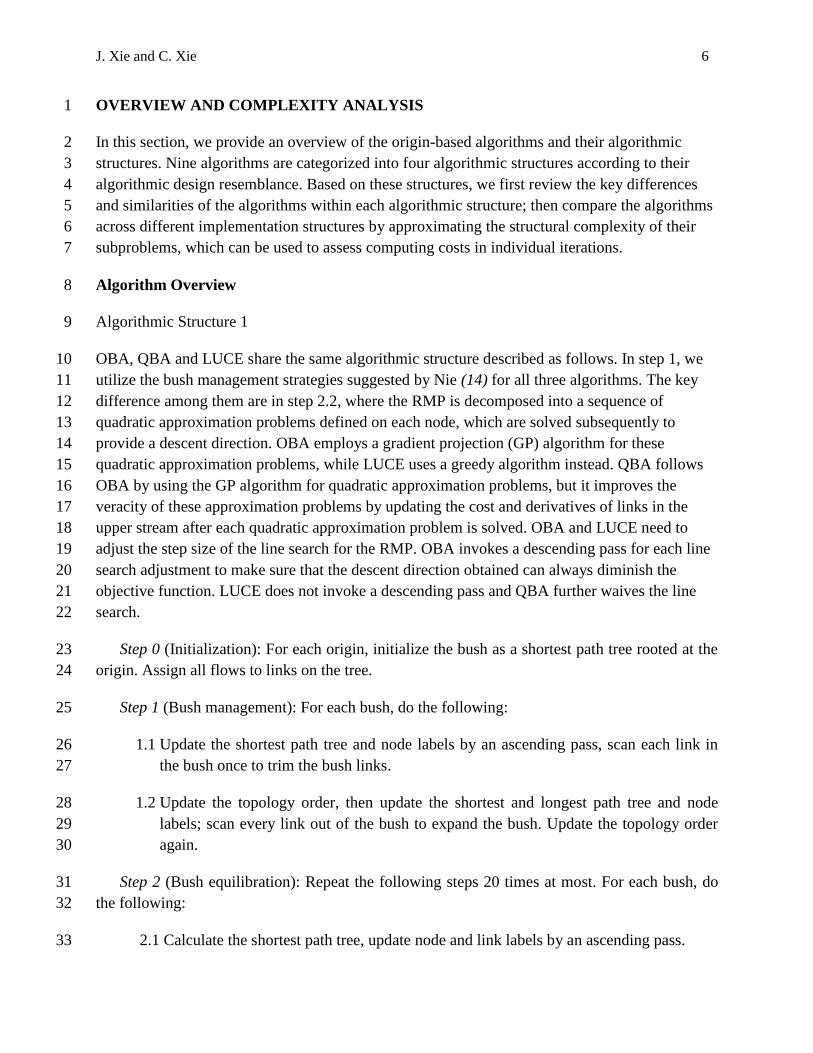
OBA, QBA and LUCE share the same algorithmic structure described as follows. In step 1, we 10

utilize the bush management strategies suggested by Nie (14) for all three algorithms. The key 11

difference among them are in step 2.2, where the RMP is decomposed into a sequence of 12

quadratic approximation problems defined on each node, which are solved subsequently to 13

provide a descent direction. OBA employs a gradient projection (GP) algorithm for these 14

quadratic approximation problems, while LUCE uses a greedy algorithm instead. QBA follows 15

OBA by using the GP algorithm for quadratic approximation problems, but it improves the 16

veracity of these approximation problems by updating the cost and derivatives of links in the 17

upper stream after each quadratic approximation problem is solved. OBA and LUCE need to 18

adjust the step size of the line search for the RMP. OBA invokes a descending pass for each line 19

search adjustment to make sure that the descent direction obtained can always diminish the 20

objective function. LUCE does not invoke a descending pass and QBA further waives the line 21

search. 22

Step 0 (Initialization): For each origin, initialize the bush as a shortest path tree rooted at the 23

origin. Assign all flows to links on the tree. 24

Step 1 (Bush management): For each bush, do the following: 25

1.1 Update the shortest path tree and node labels by an ascending pass, scan each link in 26

the bush once to trim the bush links. 27

1.2 Update the topology order, then update the shortest and longest path tree and node 28

labels; scan every link out of the bush to expand the bush. Update the topology order 29

again. 30

Step 2 (Bush equilibration): Repeat the following steps 20 times at most. For each bush, do 31

the following: 32

2.1 Calculate the shortest path tree, update node and link labels by an ascending pass. 33

J. Xie and C. Xie 7

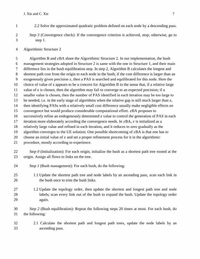
2.2 Solve the approximated quadratic problem defined on each node by a descending pass. 1

Step 3 (Convergence check): If the convergence criterion is achieved, stop; otherwise, go to 2

step 1. 3


Algorithm B and 𝜀BA share the Algorithmic Structure 2. In our implementation, the bush 5

management strategies adopted in Structure 2 is same with the one in Structure 1, and their main 6

difference lies in the bush equilibration step. In step 2, Algorithm B calculates the longest and 7

shortest path cost from the origin to each node in the bush; if the cost difference is larger than an 8

exogenously given precision 𝜀, then a PAS is searched and equilibrated for this node. Here the 9

choice of value of ε appears to be a concern for Algorithm B in the sense that, if a relative large 10

value of ε is chosen, then the algorithm may fail to converge to an expected precision; if a 11

smaller value is chosen, then the number of PAS identified in each iteration may be too large to 12

be needed, i.e. in the early stage of algorithms when the relative gap is still much larger than ε, 13

then identifying PASs with a relatively small cost difference usually make negligible effects on 14

convergence but would produce considerable computational effort. 𝜀BA proposes to 15

successively refine an endogenously determined ε value to control the generation of PAS in each 16

iteration more elaborately according the convergence needs. In 𝜀BA, 𝜀 is initialized as a 17

relatively large value and refined in each iteration, and it reduces to zero gradually as the 18

algorithm converges to the UE solution. One possible shortcoming of 𝜀BA is that one has to 19

choose an initial value of 𝜀 and set a proper refinement process for it in the algorithmic 20

procedure, mostly according to experience. 21

Step 0 (Initialization): For each origin, initialize the bush as a shortest path tree rooted at the 22

origin. Assign all flows to links on the tree. 23

Step 1 (Bush management): For each bush, do the following: 24

1.1 Update the shortest path tree and node labels by an ascending pass, scan each link in 25

the bush once to trim the bush links. 26

1.2 Update the topology order, then update the shortest and longest path tree and node 27

labels; scan every link out of the bush to expand the bush. Update the topology order 28

again. 29

Step 2 (Bush equilibration): Repeat the following steps 20 times at most. For each bush, do 30

the following: 31

2.1 Calculate the shortest path and longest path trees, update the node labels by an 32

ascending pass. 33

J. Xie and C. Xie 8

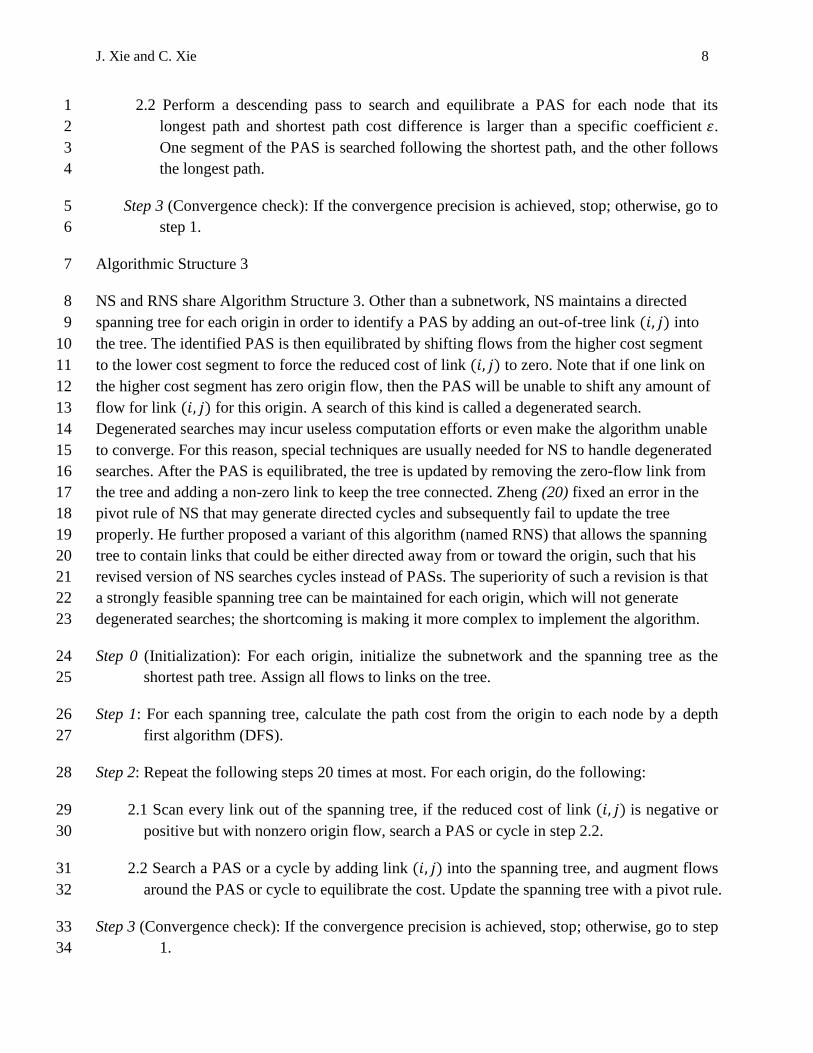
2.2 Perform a descending pass to search and equilibrate a PAS for each node that its 1

longest path and shortest path cost difference is larger than a specific coefficient 𝜀. 2

One segment of the PAS is searched following the shortest path, and the other follows 3

the longest path. 4

Step 3 (Convergence check): If the convergence precision is achieved, stop; otherwise, go to 5

step 1. 6


NS and RNS share Algorithm Structure 3. Other than a subnetwork, NS maintains a directed 8

spanning tree for each origin in order to identify a PAS by adding an out-of-tree link (𝑖, 𝑗) into 9

the tree. The identified PAS is then equilibrated by shifting flows from the higher cost segment 10

to the lower cost segment to force the reduced cost of link (𝑖, 𝑗) to zero. Note that if one link on 11

the higher cost segment has zero origin flow, then the PAS will be unable to shift any amount of 12

flow for link (𝑖, 𝑗) for this origin. A search of this kind is called a degenerated search. 13

Degenerated searches may incur useless computation efforts or even make the algorithm unable 14

to converge. For this reason, special techniques are usually needed for NS to handle degenerated 15

searches. After the PAS is equilibrated, the tree is updated by removing the zero-flow link from 16

the tree and adding a non-zero link to keep the tree connected. Zheng (20) fixed an error in the 17

pivot rule of NS that may generate directed cycles and subsequently fail to update the tree 18

properly. He further proposed a variant of this algorithm (named RNS) that allows the spanning 19

tree to contain links that could be either directed away from or toward the origin, such that his 20

revised version of NS searches cycles instead of PASs. The superiority of such a revision is that 21

a strongly feasible spanning tree can be maintained for each origin, which will not generate 22

degenerated searches; the shortcoming is making it more complex to implement the algorithm. 23

Step 0 (Initialization): For each origin, initialize the subnetwork and the spanning tree as the 24

shortest path tree. Assign all flows to links on the tree. 25

Step 1: For each spanning tree, calculate the path cost from the origin to each node by a depth 26

first algorithm (DFS). 27

Step 2: Repeat the following steps 20 times at most. For each origin, do the following: 28

2.1 Scan every link out of the spanning tree, if the reduced cost of link (𝑖, 𝑗) is negative or 29

positive but with nonzero origin flow, search a PAS or cycle in step 2.2. 30

2.2 Search a PAS or a cycle by adding link (𝑖, 𝑗) into the spanning tree, and augment flows 31

around the PAS or cycle to equilibrate the cost. Update the spanning tree with a pivot rule. 32

Step 3 (Convergence check): If the convergence precision is achieved, stop; otherwise, go to step 33

1. 34

J. Xie and C. Xie 9


TAPAS and iTAPAS share Algorithmic Structure 4. TAPAS systematically explores the use of 2

PAS for solving TAP and its three notable innovations are summarized as follows: (1) it employs 3

a breadth first search method to identify PASs directly from the shortest path tree rooted at each 4

origin at step 1.2; (2) it stores PASs in a list in order to save the time spent on repeatedly 5

identifying same segments at step 1.2; (3) it connects multiple origins to one PAS by matching 6

an origin to an existing PAS in the list, which helps secure a unique path solution by forcing 7

proportionality. Xie and Xie examined the TAPAS algorithm in great detail and found its several 8

issues related to the identification and operations of PASs that may affect the overall algorithm 9

convergence efficiency, including: (1) the breadth first search method chooses the higher cost 10

segment arbitrarily, which could lead to unpredictable and inconsistent behavior; (2) the breadth 11

first search method may fail to identify a PAS successfully if a flow effective factor is imposed, 12

such that the algorithm convergence cannot be guaranteed unless an additional branch shift 13

operation is conducted; (3) the association of multiple origins with one PAS may incur a large 14

number of link flow operations that lag the algorithm convergence in solving large, congested 15

networks. The resulting improved algorithm is named iTAPAS, which differs TAPAS mainly in 16

the following aspects: (1) a new PAS identification method which is easier, faster and more 17

effective is proposed to instead the breadth first search method and the branch shift operation. 18

The new method identifies the higher cost segment continuously with the maximum flow link in 19

the backward set of the node that starts from tail node of the target link to the origin; (2) only one 20

origin is related to each PAS in step 1.2 in the algorithm convergence process and a post-21

processing can be added to achieve the proportionality. Implementation of iTAPAS becomes 22

significantly easier than that of TAPAS. 23

Step 0 (Initialization): For each origin, initialize the subnetwork as the shortest path tree. Assign 24

all flows to links on the tree. 25

Step 1: For each origin, do the following: 26

1.1 Calculate the shortest path tree rooted at the origin. 27

1.2 Scan each link out of the tree: if the origin link flow is larger than 0 and the reduced 28

cost is smaller than 0, match an existing PAS from the PAS list for this link; if an 29

existing PAS is not matched, identify a new PAS based on the shortest path tree. 30

Equilibrate the segments cost once for the new identified PAS and save it into the PAS 31

list if both segments still have positive flows. 32

1.3 Select a number of PASs (say, 400) from the PAS list and equilibrate the segments cost 33

once. 34

J. Xie and C. Xie 10

Step 2: Repeat the following step 20 times at most: scan each PAS in the list, if the flow 1

(contributed by all associated origins) on one segment reduces to 0, delete it from the 2

PAS list; otherwise, equilibrate the segments cost once for this PAS. 3

Complexity Analysis 4

Given the above structures, the algorithms accommodated by the same structure tend to share 5

more common features than those in different structures. Here we propose to evaluate the 6

structural complexity of different algorithmic structures in each iteration by estimating the 7

frequency that they scan the set of nodes and links, which are usually the most expensive step in 8

TAP algorithms. Such a complexity analysis provides us with helpful insights of how many the 9

computation efforts are needed to conduct one algorithmic iteration by different algorithmic 10

structures. Table 1 reports the structural complexity of different algorithmic structures. Note that 11

scanning a general network is commonly more expensive than scanning a bush or a tree. Here we 12

do not distinguish them because the scanning process involves link flow and cost operations that 13

usually spread over the whole node set and link set, so the structural complexity difference 14

caused by different network topology is negligible. Let 𝑅 denote the number of origins, and 𝑃 15

denotes the number of PASs. Structure 1 and Structure 2 share the same bush management 16

strategies, so the structural complexity of step 1 for both two structures are 6𝑅. We roughly 17

estimate the structural complexity of the bush equilibration (step 2) in Structure 1 as 40𝑅 and 18

that in Structure 2 as 20𝑅, respectively. We employ a fast implementation strategy suggested by 19

(18) for B and 𝜀BA, such that over 50% of the network scanning usually can be omitted in the 20

Structure 2. Structure 3 only scans the network once for each origin in step 2 such that its 21

structural complexity is estimated as 20𝑅. The structure of TAPAS and iTAPAS has one major 22

difference from the other three structures that it stores PASs into a list in step 1 and subsequently 23

obviates scanning over the network in step 2. When the number of PASs in the list is smaller 24

than the node set size, Structure 4 spends less computational efforts than that of Structure 3; as 25

the PAS list size increases to a size that is comparable to that of nodes or links, then the 26

computational effort of Structure 4 is roughly equal or even larger than that of Structure 3. 27

Note that the structural complexity estimation cannot reflect the algorithm convergent efficiency 28

unless we further know the average convergence magnitude achieved by each iteration. Actually, 29

these two parts are subject to a tradeoff in designing a TAP algorithm. Take Algorithm B 30

described in Structure 2 as an example, a larger number of repetitions of bush equilibration will 31

invoke more ascending and descending passes of the bush and thus increase the computation 32

time of each iteration, but it also will let the RMP more converged. Even though, the complexity 33

analysis is still very useful in explaining our numerical experiments results and making our 34

comparison results more convincible in next section, where the average computation times and 35

the average convergence magnitude per iteration can be calculated based on the assignment 36

results. 37


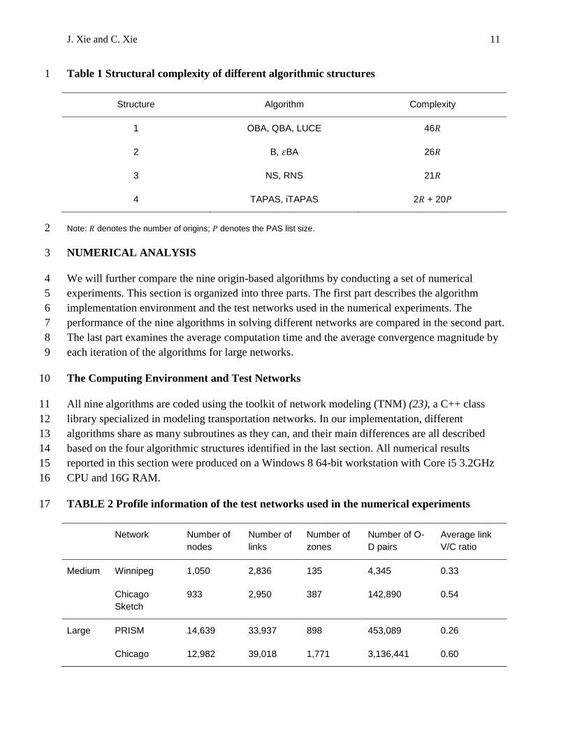
Table 1 Structural complexity of different algorithmic structures 1

Structure Algorithm Complexity

1 OBA, QBA, LUCE 46𝑅

2 B, 𝜀BA 26𝑅

3 NS, RNS 21𝑅

4 TAPAS, iTAPAS 2𝑅 + 20𝑃

Note: 𝑅 denotes the number of origins; 𝑃 denotes the PAS list size. 2

NUMERICAL ANALYSIS 3

We will further compare the nine origin-based algorithms by conducting a set of numerical 4

experiments. This section is organized into three parts. The first part describes the algorithm 5

implementation environment and the test networks used in the numerical experiments. The 6

performance of the nine algorithms in solving different networks are compared in the second part. 7

The last part examines the average computation time and the average convergence magnitude by 8

each iteration of the algorithms for large networks. 9

The Computing Environment and Test Networks 10

All nine algorithms are coded using the toolkit of network modeling (TNM) (23), a C++ class 11

library specialized in modeling transportation networks. In our implementation, different 12

algorithms share as many subroutines as they can, and their main differences are all described 13

based on the four algorithmic structures identified in the last section. All numerical results 14

reported in this section were produced on a Windows 8 64-bit workstation with Core i5 3.2GHz 15

CPU and 16G RAM. 16

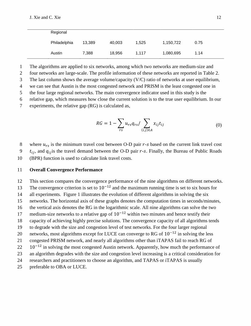
TABLE 2 Profile information of the test networks used in the numerical experiments 17

Network Number of

nodes

Number of

links

Number of

zones

Number of O-

D pairs

Average link

V/C ratio

Medium Winnipeg 1,050 2,836 135 4,345 0.33

Chicago

Sketch

933 2,950 387 142,890 0.54

Large PRISM 14,639 33,937 898 453,089 0.26

Chicago 12,982 39,018 1,771 3,136,441 0.60


Regional

Philadelphia 13,389 40,003 1,525 1,150,722 0.75

Austin 7,388 18,956 1,117 1,080,695 1.14

The algorithms are applied to six networks, among which two networks are medium-size and 1

four networks are large-scale. The profile information of these networks are reported in Table 2. 2

The last column shows the average volume/capacity (V/C) ratio of networks at user equilibrium, 3

we can see that Austin is the most congested network and PRISM is the least congested one in 4

the four large regional networks. The main convergence indicator used in this study is the 5

relative gap, which measures how close the current solution is to the true user equilibrium. In our 6

experiments, the relative gap (RG) is calculated as, 7

𝑅𝐺 = 1 −∑𝑢𝑟𝑠𝑞𝑟𝑠/ ∑ 𝑥𝑖𝑗𝑡𝑖𝑗(𝑖,𝑗)∈𝐴𝑟𝑠

(0)

where 𝑢𝑟𝑠 is the minimum travel cost between O-D pair 𝑟-𝑠 based on the current link travel cost 8

𝑡𝑖𝑗, and 𝑞𝑖𝑗is the travel demand between the O-D pair 𝑟-𝑠. Finally, the Bureau of Public Roads 9

(BPR) function is used to calculate link travel costs. 10

Overall Convergence Performance 11

This section compares the convergence performance of the nine algorithms on different networks. 12

The convergence criterion is set to 10−12 and the maximum running time is set to six hours for 13

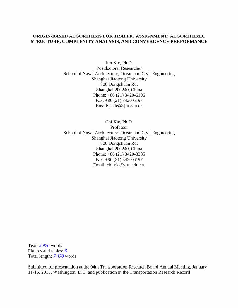
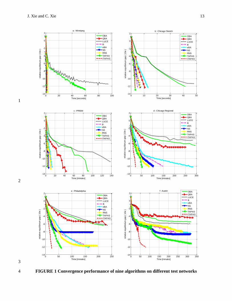
all experiments. Figure 1 illustrates the evolution of different algorithms in solving the six 14

networks. The horizontal axis of these graphs denotes the computation times in seconds/minutes, 15

the vertical axis denotes the RG in the logarithmic scale. All nine algorithms can solve the two 16

medium-size networks to a relative gap of 10−12 within two minutes and hence testify their 17

capacity of achieving highly precise solutions. The convergence capacity of all algorithms tends 18

to degrade with the size and congestion level of test networks. For the four larger regional 19

networks, most algorithms except for LUCE can converge to RG of 10−12 in solving the less 20

congested PRISM network, and nearly all algorithms other than iTAPAS fail to reach RG of 21

10−12 in solving the most congested Austin network. Apparently, how much the performance of 22

an algorithm degrades with the size and congestion level increasing is a critical consideration for 23

researchers and practitioners to choose an algorithm, and TAPAS or iTAPAS is usually 24

preferable to OBA or LUCE. 25


1

2

3

FIGURE 1 Convergence performance of nine algorithms on different test networks 4

0 20 40 60 80 100-14

-12

-10

-8

-6

-4

-2

0

2a : Winnipeg

rela

tive

eq

uilib

riu

m g

ap

( 1

0e

)

Time [seconds]

OBA

QBA

LUCE

B

eBA

NS

RNS

TAPAS

iTAPAS

0 10 20 30 40 50-14

-12

-10

-8

-6

-4

-2

0

2b : Chicago Sketch

rela

tive

eq

uilib

riu

m g

ap

( 1

0e

)

Time [seconds]

OBA

QBA

LUCE

B

eBA

NS

RNS

TAPAS

iTAPAS

0 20 40 60 80 100 120 140-14

-12

-10

-8

-6

-4

-2

0

2c : PRISM

rela

tive

eq

uilib

riu

m g

ap

( 1

0e

)

Time [minutes]

OBA

QBA

LUCE

B

eBA

NS

RNS

TAPAS

iTAPAS

0 50 100 150 200 250 300-14

-12

-10

-8

-6

-4

-2

0

2d : Chicago Regional

rela

tive

eq

uilib

riu

m g

ap

( 1

0e

)

Time [minutes]

OBA

QBA

LUCE

B

eBA

NS

RNS

TAPAS

iTAPAS

0 50 100 150 200 250-14

-12

-10

-8

-6

-4

-2

0

2e : Philadelphia

rela

tive

eq

uilib

riu

m g

ap

( 1

0e

)

Time [minutes]

OBA

QBA

LUCE

B

eBA

NS

RNS

TAPAS

iTAPAS

0 50 100 150 200 250 300 350-14

-12

-10

-8

-6

-4

-2

0

2f : Austin

rela

tive

eq

uilib

riu

m g

ap

( 1

0e

)

Time [minutes]

OBA

QBA

LUCE

B

eBA

NS

RNS

TAPAS

iTAPAS


Particularly, iTAPAS is found to be the algorithm with the best performance in all cases, and 1

TAPAS follows as the second best algorithm. Note that iTAPAS can be two times faster than 2

TAPAS in solving the Chicago Regional, Philadelphia and Austin networks, and this may 3

attributes to the new PAS identification method and the simplified PAS flow operations of 4

iTAPAS. NS, RNS, Algorithm B and εBA perform similarly in our test. RNS may outperform 5

the other three slightly if examined closely. NS stops to converge further at RG of 10−8 in 6

solving the Philadelphia and Austin networks for unclear reasons. OBA, QBA and LUCE 7

perform less efficiently than the other six algorithms to a large extent, mainly due to their 8

unfaithful approximation of RMP into a sequence of quadratic node problems. The reader is 9

referred to (24) for detailed discussions about these three algorithms. 10

Convergence Performance per Iteration 11

In this section, we will further explore the assignment results, particularly in several per-iteration 12

statistics, in order to provide more comparisons in the convergence behavior of different 13

algorithms, and to give possible explanations for the degradation effects of algorithms with 14

network size and congestion level. Recall that the overall convergence of algorithms can be 15

determined by two aspects: the average computation time per iteration and the average 16

convergence magnitude per iteration. Given the assignments results, we can easily calculate the 17

average computation time of one iteration for each algorithm on a specific network. Here we 18

further define an indicator 𝑀 to measure the average convergence magnitude of each iteration as 19

follows: 20

𝑀 =∑ (𝑙𝑜𝑔𝑅𝐺𝑘 − 𝑙𝑜𝑔𝑅𝐺𝑘+1)𝑘∈[1..𝐾−1]

𝐾 − 1 (0)

where 𝑅𝐺𝑘 denotes the relative gap defined in equation (0) on iteration 𝑘, and 𝐾 is the maximum 21

iteration index when the algorithms converge to 𝑅𝐺 of 10−12 or reach the maximum running 22

time. 23

The two computation statistics averaged by all iterations for each algorithm and each network are 24

reported in Table 3. 𝐾 denotes the total number of iterations considered, 𝑇 denotes the average 25

computation time of one iteration and 𝑀 is the convergence magnitude indicator defined above. 26

We can obtain some useful conclusions from this table. By taking the statistics of LUCE in 27

solving the Chicago Regional network as an example, we found that it takes about 18.2 minutes 28

for LUCE to achieve 𝑀 of 0.23. If we optimistically assume that 𝑇 and 𝑀 in this case will keep 29

unchanged through the whole convergence process, then it is easy to calculate that LUCE will 30

take at least 15.8 hours1 to converge to 𝑅𝐺 of 10−12 in this case. 31

1 This is calculated as [(log1 − log10−12)/0.23] × 0.303 ≈ 15.8 hours.


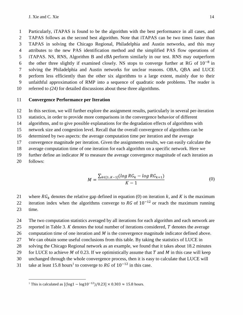
TABLE 3 Average computation time and convergence magnitude per iteration 1

Network Statistics per

iteration

Algorithm

OBA QBA LUCE B 𝜀BA NS RNS TAPAS iTAPAS

PRISM K 12 14 12 13 15 11 22 6 10

T 7.38m 3.04m 11.5m 0.76m 0.89m 0.53m 0.48m 0.44m 0.34m

M 0.816 0.902 0.695 0.776 0.644 0.881 0.472 1.90 1.26

Chicago

Regional

K 22 29 12 76 51 75 73 21 36

T 13.3m 8.13m 18.2m 1.93m 5.79m 1.36m 1.12m 2.4m 0.60m

M 0.240 0.182 0.23 0.144 0.217 0.141 0.145 0.503 0.295

Philadelphia K 18 34 20 54 43 94 79 23 26

T 16.5m 10.26m 17.3m 3.13m 3.74m 1.88m 2.43m 2.45m 0.86m

M 0.342 0.165 0.314 0.204 0.258 0.076 0.135 0.467 0.421

Austin K 50 44 74 199 145 119 199 95 133

T 7.25m 8.37m 4.83m 1.20m 2.1m 0.95m 1.36m 3.4m 0.67m

M 0.089 0.091 0.07 0.037 0.05 0.044 0.034 0.1 0.091

Note: m denotes minutes. 2

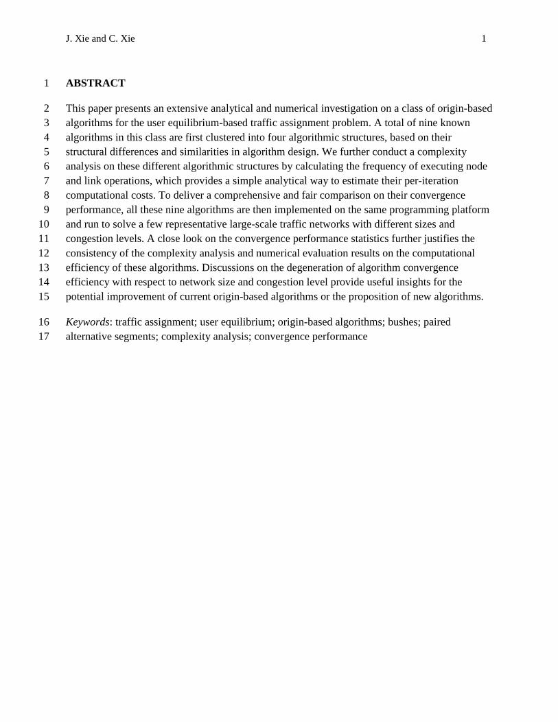
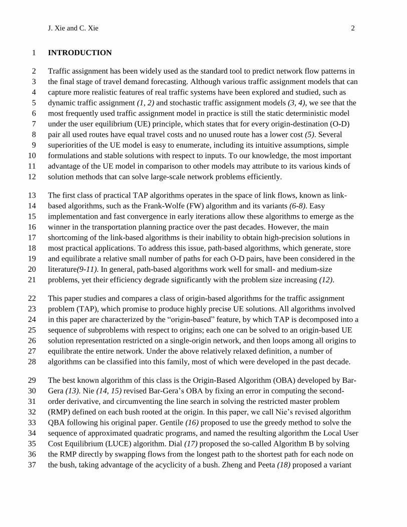
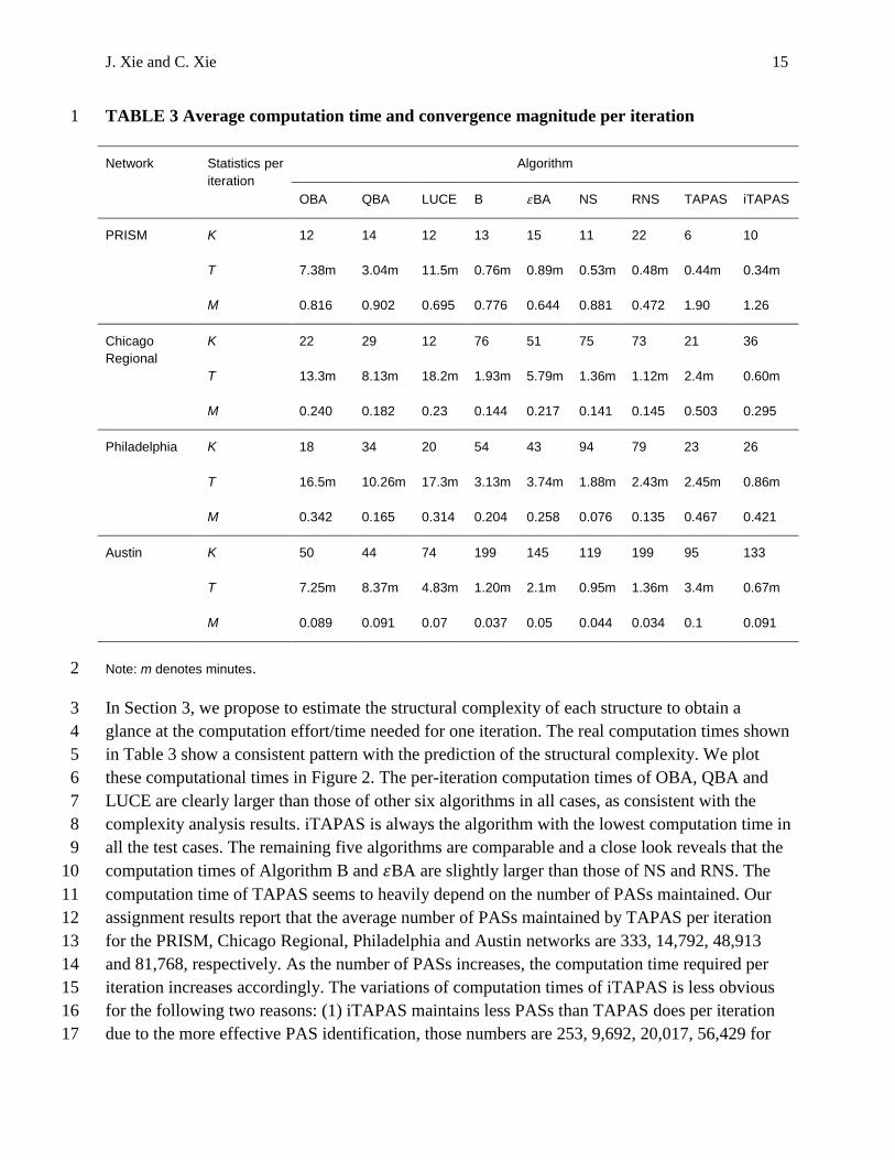
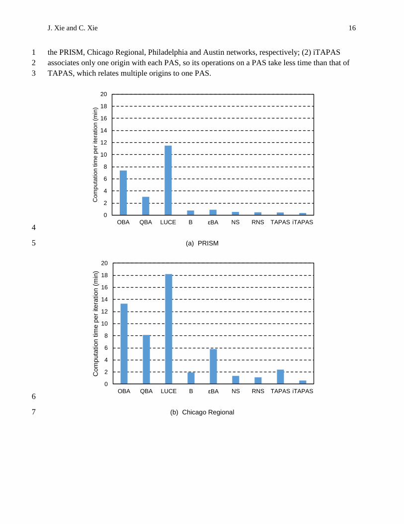
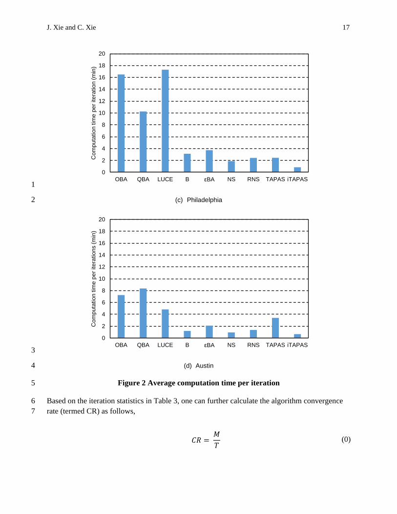
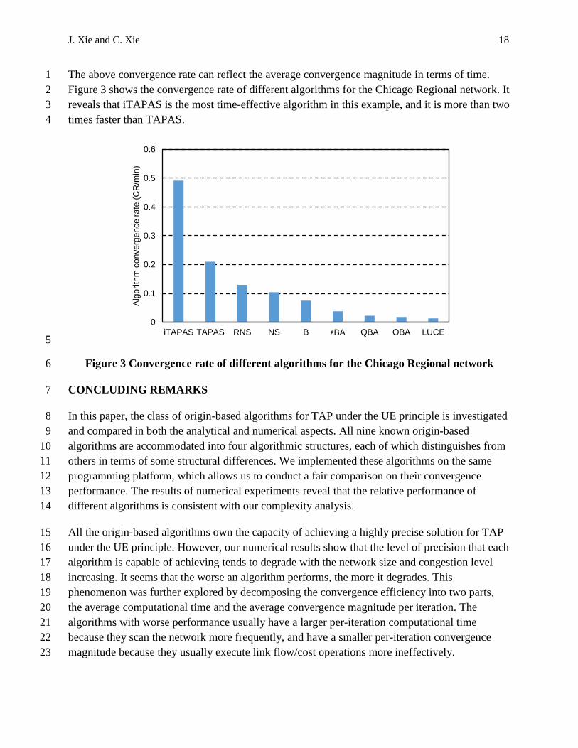
In Section 3, we propose to estimate the structural complexity of each structure to obtain a 3

glance at the computation effort/time needed for one iteration. The real computation times shown 4

in Table 3 show a consistent pattern with the prediction of the structural complexity. We plot 5

these computational times in Figure 2. The per-iteration computation times of OBA, QBA and 6

LUCE are clearly larger than those of other six algorithms in all cases, as consistent with the 7

complexity analysis results. iTAPAS is always the algorithm with the lowest computation time in 8

all the test cases. The remaining five algorithms are comparable and a close look reveals that the 9

computation times of Algorithm B and 𝜀BA are slightly larger than those of NS and RNS. The 10

computation time of TAPAS seems to heavily depend on the number of PASs maintained. Our 11

assignment results report that the average number of PASs maintained by TAPAS per iteration 12

for the PRISM, Chicago Regional, Philadelphia and Austin networks are 333, 14,792, 48,913 13

and 81,768, respectively. As the number of PASs increases, the computation time required per 14

iteration increases accordingly. The variations of computation times of iTAPAS is less obvious 15

for the following two reasons: (1) iTAPAS maintains less PASs than TAPAS does per iteration 16

due to the more effective PAS identification, those numbers are 253, 9,692, 20,017, 56,429 for 17


the PRISM, Chicago Regional, Philadelphia and Austin networks, respectively; (2) iTAPAS 1

associates only one origin with each PAS, so its operations on a PAS take less time than that of 2

TAPAS, which relates multiple origins to one PAS. 3

4

(a) PRISM 5

6

(b) Chicago Regional 7

0

2

4

6

8

10

12

14

16

18

20

OBA QBA LUCE B εBA NS RNS TAPAS iTAPAS

Com

pu

tatio

n tim

e p

er

ite

ratio

n (

min

)

0

2

4

6

8

10

12

14

16

18

20


Com

puta

tion t

ime p

er

itera

tion (

min

)


1

(c) Philadelphia 2

3

(d) Austin 4

Figure 2 Average computation time per iteration 5

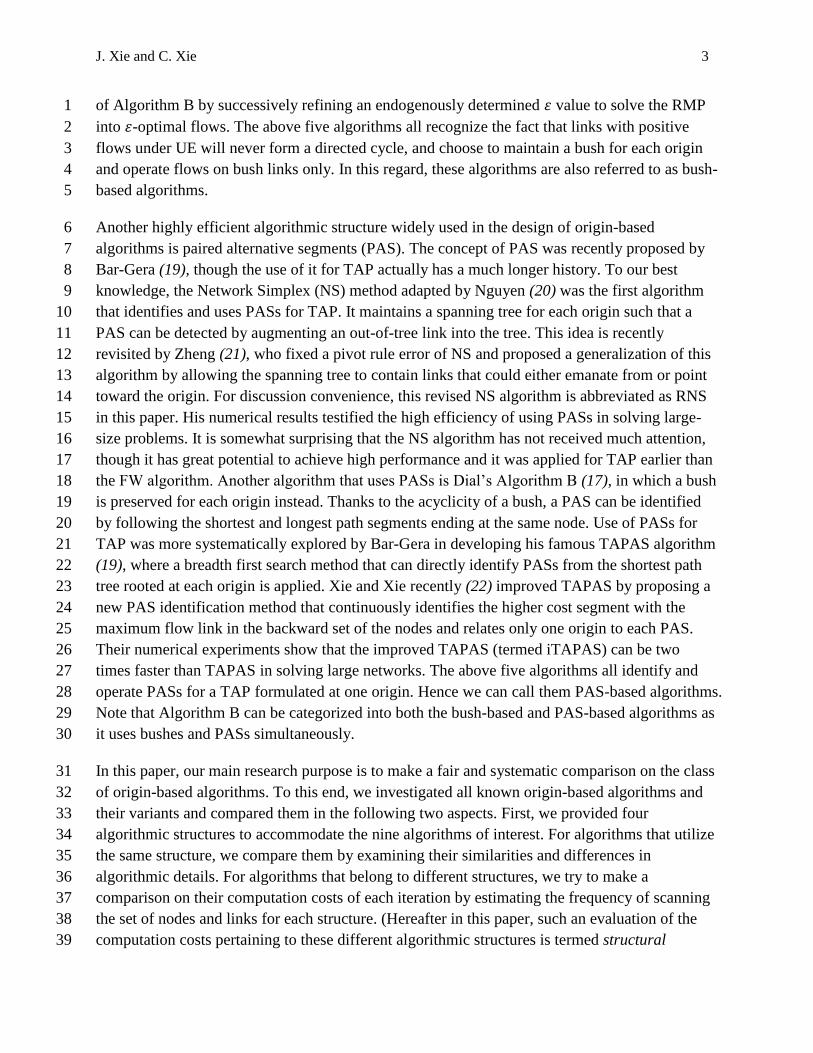
Based on the iteration statistics in Table 3, one can further calculate the algorithm convergence 6

rate (termed CR) as follows, 7

𝐶𝑅 = 𝑀

𝑇 (0)

0

2

4

6

8

10

12

14

16

18

20


Co

mp

uta

tio

n tim

e p

er

ite

ratio

n (

min

)

0

2

4

6

8

10

12

14

16

18

20


Com

pu

tatio

n tim

e p

er

ite

ratio

ns (

min

)


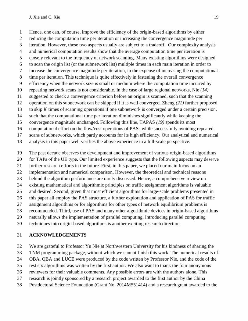
The above convergence rate can reflect the average convergence magnitude in terms of time. 1

Figure 3 shows the convergence rate of different algorithms for the Chicago Regional network. It 2

reveals that iTAPAS is the most time-effective algorithm in this example, and it is more than two 3

times faster than TAPAS. 4

5

Figure 3 Convergence rate of different algorithms for the Chicago Regional network 6

CONCLUDING REMARKS 7

In this paper, the class of origin-based algorithms for TAP under the UE principle is investigated 8

and compared in both the analytical and numerical aspects. All nine known origin-based 9

algorithms are accommodated into four algorithmic structures, each of which distinguishes from 10

others in terms of some structural differences. We implemented these algorithms on the same 11

programming platform, which allows us to conduct a fair comparison on their convergence 12

performance. The results of numerical experiments reveal that the relative performance of 13

different algorithms is consistent with our complexity analysis. 14

All the origin-based algorithms own the capacity of achieving a highly precise solution for TAP 15

under the UE principle. However, our numerical results show that the level of precision that each 16

algorithm is capable of achieving tends to degrade with the network size and congestion level 17

increasing. It seems that the worse an algorithm performs, the more it degrades. This 18

phenomenon was further explored by decomposing the convergence efficiency into two parts, 19

the average computational time and the average convergence magnitude per iteration. The 20

algorithms with worse performance usually have a larger per-iteration computational time 21

because they scan the network more frequently, and have a smaller per-iteration convergence 22

magnitude because they usually execute link flow/cost operations more ineffectively. 23

0

0.1

0.2

0.3

0.4

0.5

0.6

iTAPAS TAPAS RNS NS B εBA QBA OBA LUCE

Alg

ori

thm

co

nve

rge

nce

ra

te (

CR

/min

)


Hence, one can, of course, improve the efficiency of the origin-based algorithms by either 1

reducing the computation time per iteration or increasing the convergence magnitude per 2

iteration. However, these two aspects usually are subject to a tradeoff. Our complexity analysis 3

and numerical computation results show that the average computation time per iteration is 4

closely relevant to the frequency of network scanning. Many existing algorithms were designed 5

to scan the origin list (or the subnetwork list) multiple times in each main iteration in order to 6

increase the convergence magnitude per iteration, in the expense of increasing the computational 7

time per iteration. This technique is quite effectively in fastening the overall convergence 8

efficiency when the network size is small or medium where the computation time incurred by 9

repeating network scans is not considerable. In the case of large regional networks, Nie (14) 10

suggested to check a convergence criterion before an origin is scanned, such that the scanning 11

operation on this subnetwork can be skipped if it is well converged. Zheng (21) further proposed 12

to skip 𝐾 times of scanning operations if one subnetwork is converged under a certain precision, 13

such that the computational time per iteration diminishes significantly while keeping the 14

convergence magnitude unchanged. Following this line, TAPAS (19) spends its most 15

computational effort on the flow/cost operations of PASs while successfully avoiding repeated 16

scans of subnetworks, which partly accounts for its high efficiency. Our analytical and numerical 17

analysis in this paper well verifies the above experience in a full-scale perspective. 18

The past decade observes the development and improvement of various origin-based algorithms 19

for TAPs of the UE type. Our limited experience suggests that the following aspects may deserve 20

further research efforts in the future. First, in this paper, we placed our main focus on an 21

implementation and numerical comparison. However, the theoretical and technical reasons 22

behind the algorithm performance are rarely discussed. Hence, a comprehensive review on 23

existing mathematical and algorithmic principles on traffic assignment algorithms is valuable 24

and desired. Second, given that most efficient algorithms for large-scale problems presented in 25

this paper all employ the PAS structure, a further exploration and application of PAS for traffic 26

assignment algorithms or for algorithms for other types of network equilibrium problems is 27

recommended. Third, use of PAS and many other algorithmic devices in origin-based algorithms 28

naturally allows the implementation of parallel computing. Introducing parallel computing 29

techniques into origin-based algorithms is another exciting research direction. 30

ACKNOWLEDGEMENTS 31

We are grateful to Professor Yu Nie at Northwestern University for his kindness of sharing the 32

TNM programming package, without which we cannot finish this work. The numerical results of 33

OBA, QBA and LUCE were produced by the code written by Professor Nie, and the code of the 34

rest six algorithms was written by the first author. We also want to thank the four anonymous 35

reviewers for their valuable comments. Any possible errors are with the authors alone. This 36

research is jointly sponsored by a research project awarded to the first author by the China 37

Postdoctoral Science Foundation (Grant No. 2014M551414) and a research grant awarded to the 38


second author from the State Key Laboratory of Ocean Engineering at Shanghai Jiao Tong 1

University (Grant No. GKZD010061). 2

REFERENCES 3

1. Merchant, D. K. and G. L. Nemhauser. Model and an Algorithm for the Dynamic Traffic 4

Assignment Problems. Transportation Science, Vol. 12, No. 3, 1978, pp. 183-199. 5

2. Peeta, S. and A. K. Ziliaskopoulos. Foundations of Dynamic Traffic Assignment: The 6

Past, the Present and the Future. Networks and Spatial Economics, Vol. 1, No. 3-4, 2001, 7

pp. 233-266. 8

3. Daganzo, C. F. and Y. Sheffi. On Stochastic Models of Traffic Assignment. 9

Transportation Science, Vol. 11, No. 3, 1977, pp. 83-111. 10

4. Xie, C. and S. T. Waller. Stochastic Traffic Assignment, Lagrangian Dual, and 11

Unconstrained Convex Optimization. Transportation Research Part B: Methodological, 12

Vol. 46, No. 8, 2012, pp. 1023-1042. 13

5. Wardrop, J. G. Some Theoretical Aspects of Road Traffic Research. Proceedings of the 14

institution of Civil Engineering, Part II, Vol. 1, No. 2, 1952, pp. 325-378. 15

6. LeBlanc, L. J., E. K. Morlok and W. P. Pierskalla. An Efficient Approach to Solving the 16

Road Network Equilibrium Traffic Assignment Problem. Transportation Research, Vol. 17

9, No. 5, 1975, pp. 309-318. 18

7. Florian, M., J. Guálat and H. Spiess. An Efficient Implementation of the “Partan” Variant 19

of the Linear Approximation Method for the Network Equilibrium Problem. Networks, 20

Vol. 17, No. 3, 1987, pp. 319-339. 21

8. Fukushima, M. A Modified Frank-Wolfe Algorithm for Solving the Traffic Assignment 22

Problem. Transportation Research Part B: Methodological, Vol. 18, No. 2, 1984, pp. 23

169-177. 24

9. Larsson, T. and M. Patriksson. Simplicial Decomposition with Disaggregated 25

Representation for the Traffic Assignment Problem. Transportation Science, Vol. 26, No. 26

1, 1992, pp. 4-17. 27

10. Jayakrishnan, R., W. T. Tsai, J. N. Prashker and S. Rajadhyaksha. A Faster Path-Based 28

Algorithm for Traffic Assignment. Transportation Research Record: Journal of the 29

Transportation Research Board, No. 1443, 1994, pp. 75-83. 30

11. Florian, M., I. Constantin and D. Florian. A New Look at Projected Gradient Method for 31

Equilibrium Assignment. Transportation Research Record: Journal of the 32

Transportation Research Board, No. 2090, 2009, pp. 10-16. 33

12. Inoue, S. and T. Maruyama. Computational Experience on Advanced Algorithms for 34

User Equilibrium Traffic Assignment Problem and Its Convergence Error. The 8th 35

International Conference on Traffic and Transportation Studies, Vol. 43, Changsha, 36

China, 2012, pp. 445-456. 37

13. Bar-Gera, H. Origin-Based Algorithm for the Traffic Assignment Problem. 38

Transportation Science, Vol. 36, No. 4, 2002, pp. 398-417. 39

14. Nie, Y. M. A Class of Bush-Based Algorithms for the Traffic Assignment Problem. 40

Transportation Research Part B: Methodological, Vol. 44, No. 1, 2010, pp. 73-89. 41

15. Nie, Y. M. A Note on Bar-Gera's Algorithm for the Origin-Based Traffic Assignment 42

Problem. Transportation Science, Vol. 46, No. 1, 2012, pp. 27-38. 43


16. Gentile, G. Local User Cost Equilibrium: A Bush-Based Algorithm for Traffic 1

Assignment. Transportmetrica, 2012. (In press) 2

17. Dial, R. B. A Path-Based User-Equilibrium Traffic Assignment Algorithm That Obviates 3

Path Storage and Enumeration. Transportation Research Part B: Methodological, Vol. 4

40, No. 10, 2006, pp. 917-936. 5

18. Zheng, H. and S. Peeta. Cost Scaling Based Successive Approximation Algorithm for the 6

Traffic Assignment Problem. Transportation Research Part B: Methodological, Vol. 68, 7

2014, pp. 17-30. 8

19. Bar-Gera, H. Traffic Assignment by Paired Alternative Segments. Transportation 9

Research Part B: Methodological, Vol. 44, No. 8, 2010, pp. 1022-1046. 10

20. Nguyen, S. An Algorithm for the Traffic Assignment Problem. Transportation Science, 11

Vol. 8, No. 3, 1974, pp. 203-216. 12

21. Zheng, H. Adaptation of Network Simplex for the Traffic Assignment Problem. 13

Transportation Science, 2014. (In review) 14

22. Xie, J. and C. Xie. An Improved TAPAS Algorithm for the Traffic Assignment Problem. 15

Proceedings of the 17th International IEEE Conference on Intelligent Transportation, 16

Qingdao, China, 2014. 17

23. Nie, Y. A Programmer’s Manual for Toolkit of Network Modeling (TNM). Department of 18

Civil and Environmental Engineering, University of California, Davis, CA, 2006. 19

24. Xie, J., Y. M. Nie and X. Yang. Quadratic Approximation and Convergence of Some 20

Bush-Based Algorithms for the Traffic Assignment Problem. Transportation Research 21

Part B: Methodological, Vol. 56, 2013, pp. 15-30. 22

23

origin-based algorithms for traffic assignment: algorithmic structure, complexity...

Documents