origami antennas for novel reconfigurable communication

Florida International UniversityFIU Digital Commons

FIU Electronic Theses and Dissertations University Graduate School

3-21-2018

Origami Antennas for Novel ReconfigurableCommunication SystemsXueli LiuFlorida International University, [email protected]

DOI: 10.25148/etd.FIDC004091Follow this and additional works at: https://digitalcommons.fiu.edu/etd

Part of the Electrical and Electronics Commons, and the Electromagnetics and PhotonicsCommons

This work is brought to you for free and open access by the University Graduate School at FIU Digital Commons. It has been accepted for inclusion inFIU Electronic Theses and Dissertations by an authorized administrator of FIU Digital Commons. For more information, please contact [email protected].

Recommended CitationLiu, Xueli, "Origami Antennas for Novel Reconfigurable Communication Systems" (2018). FIU Electronic Theses and Dissertations.3644.https://digitalcommons.fiu.edu/etd/3644

https://digitalcommons.fiu.edu/?utm_source=digitalcommons.fiu.edu%2Fetd%2F3644&utm_medium=PDF&utm_campaign=PDFCoverPages

https://digitalcommons.fiu.edu/etd?utm_source=digitalcommons.fiu.edu%2Fetd%2F3644&utm_medium=PDF&utm_campaign=PDFCoverPages

https://digitalcommons.fiu.edu/ugs?utm_source=digitalcommons.fiu.edu%2Fetd%2F3644&utm_medium=PDF&utm_campaign=PDFCoverPages

https://digitalcommons.fiu.edu/etd?utm_source=digitalcommons.fiu.edu%2Fetd%2F3644&utm_medium=PDF&utm_campaign=PDFCoverPages

http://network.bepress.com/hgg/discipline/270?utm_source=digitalcommons.fiu.edu%2Fetd%2F3644&utm_medium=PDF&utm_campaign=PDFCoverPages



https://digitalcommons.fiu.edu/etd/3644?utm_source=digitalcommons.fiu.edu%2Fetd%2F3644&utm_medium=PDF&utm_campaign=PDFCoverPages

mailto:[email protected]

FLORIDA INTERNATIONAL UNIVERSITY

Miami, Florida

ORIGAMI ANTENNAS FOR NOVEL RECONFIGURABLE COMMUNICATION

SYSTEMS

A dissertation submitted in partial fulfillment of

the requirements for the degree of

DOCTOR OF PHILOSOPHY

in

ELECTRICAL ENGINEERING

by

Xueli Liu

2018

ii

To: Dean John L. Volakis

College of Engineering and Computing

This dissertation, written by Xueli Liu, and entitled Origami Antennas for Novel

Reconfigurable Communication Systems, having been approved in respect to style and

intellectual content, is referred to you for judgment.

We have read this dissertation and recommend that it be approved.

_______________________________________

Nezih Pala

_______________________________________

Jean H. Andrian

_______________________________________

Berrin Tansel

_______________________________________

Kang Yen

_______________________________________

Stavros V. Georgakopoulos, Major Professor

Date of Defense: March 21, 2018.

The dissertation of Xueli Liu is approved.

_______________________________________

Dean John L. Volakis

College of Engineering and Computing

_______________________________________

Andres G. Gil

Vice President for Research and Economic Development

and Dean of the University Graduate School

Florida International University, 2018

iii

© Copyright 2017 by Xueli Liu

All rights reserved.

iv

DEDICATION

I dedicate this dissertation to my family, especially my dear husband. Without their

love, understanding and support, the completion of this work would never have been

achievable.

v

ACKNOWLEDGMENTS

I would like to express my sincerest gratitude to my major professor, Dr. Stavros

V. Georgakopoulos, for his great mentoring and relentless support through my Ph.D.

program at FIU. He provided the most excellent research environment with the latest

research software and top advanced equipment. His hard-working, gentle and earnest way

of life and research sets up a role model for me, and I sincerely thank him for his

constructive academic advices, graceful patience and understanding during these five

important years of my life. He has truly given me the confidence and knowledge base to

excel in the next stage of my career. I also appreciate Dr. Nezih Pala, Dr. Jean H. Andrian,

Dr. Berrin Tansel, and Dr. Kang Yen for serving on my dissertation defense committee and

for their illuminating comments.

I am sincerely thankful for my husband who encouraged me throughout the

research. Thanks for his and my parents’ inspiration, love, understanding, encouragement

and advices. I also thank all the members of FIU Electrical and Computing Engineering

Department and special thanks to Dr. Hao Hu, Dr. Shun Yao, Kun Bao, Daerhan Liu, John

Gibson, Karina Quintana, Elad Siman Tov, Pablo Gonzalez, Yonathan Bonan, Dr. Yipeng

Qu, Ms. Xiang Li, and Mr. Oscar Silveira for their help and friendship.

Finally, I would like to greatly thank the Graduate School of FIU for awarding me

the Dissertation Year Fellowship, which supported me in the last year of my Ph.D. research.

I would also like to recognize the supported by the National Science Foundation and

Northrop Grumman for their support of this work.

vi

ABSTRACT OF THE DISSERTATION

ORIGAMI ANTENNAS FOR NOVEL RECONFIGURABLE COMMUNICATION

SYSTEMS

by

Xueli Liu

Florida International University, 2017

Miami, Florida

Professor Stavros. V. Georgakopoulos, Major Professor

Antennas play a crucial role in communication systems since they are the

transmitting/receiving elements that transition information from guided transmission to

open-space propagation. Antennas are used in many different applications such as

aerospace communications, mobile phones, TVs and radios. Since the dimensions of

antennas are usually physically proportional to the wavelength at their operating

frequencies, it is important to develop large antennas and arrays that can be stowed

compactly and easily deployed. Also, it is important to minimize the number of antennas

on a platform by developing multifunctional antennas.

The first aim of this research is to develop new deployable, collapsible, light-weight

and robust reconfigurable antennas based on origami principles. All designs will be

validated through simulations and measurements. Paper as well as other substrates, such

as, Kapton and fabric, will be used to develop our origami antennas. The second aim of

this research is to derive integrated analytical and simulation models for designing optimal

origami antennas for various applications, such as, satellite or ground communications.

vii

This dissertation presents research on origami antennas for novel reconfigurable

communication systems. New designs of reconfigurable monofilar, bifilar and quadrifilar

antennas based on origami cylinders are developed and validated. Novel fabrication

methods of origami antennas are presented with detailed geometrical analysis. Furthermore,

multi-radii origami antennas are proposed, analyzed, fabricated and validated and they

exhibit improved circular polarization performance and wide bandwidths. An actuation

mechanism is designed for these antennas. For the first time, a low-cost and lightweight

reconfigurable origami antenna with a reflector is developed here. In addition, an array is

developed using this antenna as its element. Finally, a kresling conical spiral antenna and

a spherical helical antenna are designed with mode reconfigurabilities.

viii

TABLE OF CONTENTS

CHAPTER PAGE

Contents

1 INTRODUCTION ........................................................................................................ 1

1.1 Problem Statement ................................................................................................... 1

1.2 Research Objectives and Contributions ................................................................... 2

1.3 Methodology ............................................................................................................ 3

1.4 Dissertation Outline .................................................................................................. 3

2 BACKGROUND AND RELATED WORK ................................................................ 5

2.1 Origami Art .............................................................................................................. 5

2.2 Reconfigurable Antennas ......................................................................................... 5

3 ORIGAMI HELICAL ANTENNA............................................................................... 7

3.1 Standard Axial Mode Helical Monofilar Antenna ................................................... 7

3.2 Analysis of Origami Helical Model ......................................................................... 8

3.3 Comparison of Standard Helical Antennas with Equivalent Origami Helical

Antennas ................................................................................................................. 12

3.4 Reconfigurable Helical Antenna Based on Origami Neoprene with High

Radiation Efficiency ............................................................................................... 19

3.4.1 Antenna Geometry ............................................................................................ 19

3.4.2 Prototype of the Helical Antenna ...................................................................... 21

3.4.3 Simulated and Measured Results ...................................................................... 21

3.5 Reconfigurable Origami Bifilar Helical Antenna .................................................. 24

3.6 Frequency Reconfigurable QHA Based on Kapton Origami Helical Tube for

GPS, Radio and Wimax Applications .................................................................... 31

3.6.1 Analysis of origami structures of QHA ............................................................ 31

3.6.2 Helical and Bellow origami tube QHAs ........................................................... 33

3.6.3 Prototypes and Results of Helical Tube Based QHA ....................................... 36

3.6.4 Conclusion ........................................................................................................ 40

4 A RECONFIGURABLE PACKABLE AND MULTIBAND ORIGAMI MULTI-

RADII HELICAL ANTENNA ................................................................................... 41

4.1 Geometries of Origami Base .................................................................................. 41

4.2 Geometries of Antenna Model ............................................................................... 44

4.3 Comparison of Origami Multi-Radii Monofilar with Standard and Origami

Helices .................................................................................................................... 49

4.3.1 Comparison of Origami Multi-Radii Monofilar with Standard Helix .............. 49

4.3.2 Performance Comparison of Reconfigurable Origami Multi-Radii

Monofilar with Previous Origami Monofilar ................................................... 53

4.4 Parametric Analysis of the Origami Multi-radii Helical Antenna ......................... 58

4.4.1 Determining Parameter a1 of the Top Helix ...................................................... 58

4.4.2 Determining the Number of Turns of the Large Helix ..................................... 60

ix

4.4.3 Determining the Number of Turns of the Small Helix ..................................... 60

4.4.4 Spacing between Adjacent Turns of Bottom Helix .......................................... 61

4.4.5 Spacing between Adjacent Turns of Top Monofilar-S1 .................................... 62

4.5 Fabrication of Antenna and Actuation Mechanism ................................................ 64

4.5.1 Fabrication of the Origami Multi-Radii Helix .................................................. 64

4.5.2 Fabrication of the Actuating Mechanism .......................................................... 65

4.6 Simulated and Measured Results ........................................................................... 66

4.7 Conclusions ............................................................................................................ 72

5 REFLECTOR RECONFIGURABLE ORIGAMI QUADRIFILAR AND

MONOFILAR HELICAL ANTENNA FOR SATELLITE

COMMUNICATIONS ............................................................................................... 73

5.1 Origami QHA with Reflector ................................................................................. 73

5.1.1 Design of Origami QHA ................................................................................... 73

5.1.2 Design of the Origami Reflector ....................................................................... 75

5.1.3 Simulation Results ............................................................................................ 76

5.1.4 10:1 Scale Model of Origami QHA .................................................................. 79

5.1.5 Conclusion ........................................................................................................ 83

5.2 Tri-band Reconfigurable Origami Helical Array ................................................... 84

5.2.1 Geometry of Single Helical Antenna Element.................................................. 84

5.2.2 Geometry of Single Reflector Element ............................................................. 84

5.2.3 Geometry of 7-element Array ........................................................................... 85

5.2.4 Fabrication of Prototype ................................................................................... 86

5.2.5 Simulated and Measured Results ...................................................................... 86

6 OTHER ORIGAMI ANTENNA STRUCTURES ...................................................... 88

6.1 Mode Reconfigurable Bistable Spiral Antenna Based on Kresling Origami ......... 88

6.1.1 Kresling Conical or Cylindrical Origami .......................................................... 88

6.1.2 Simulated Results.............................................................................................. 90

6.2 A Frequency Tunable Origami Spherical Helical Antenna .................................... 91

6.2.1 Origami Pattern ................................................................................................. 92

6.2.2 Simulated Model and Results ........................................................................... 93

6.2.3 Conclusion ........................................................................................................ 94

7 CONCLUSION AND FUTURE WORK ................................................................... 95

7.1 Conclusions ............................................................................................................ 95

7.2 Future Work ........................................................................................................... 95

REFERENCES ........................................................................................................... 97

VITA ......................................................................................................................... 102

x

LIST OF TABLES

TABLE PAGE

Table 3.1 Empirical Optimum Parameters of Monofilar Helical Antenna...........................8

Table 3.2 Geometric Parameters of Origami Helical Antennas.........................................11

Table 3.3 Relationships between Standard and Origami Helices.......................................12

Table 3.4 Geometric Parameters of the Standard Helical Antenna....................................12

Table 3.5 Calculated Parameters of Equivalent Origami Helical Antennas with

Different Folding Patterns.................................................................................13

Table 3.6 Performance Comparison of Standard Helical Monofilar Antenna and

Its Equivalent Origami Helical Monofilar Antennas.........................................15

Table 3.7 Values of Geometrical Parameters of the Antenna.............................................20

Table 3.8 Summarized Measured Results of The Antenna.................................................24

Table 3.9 Measured Realized Gain (dB) at the Operating Frequencies of the 3 States

of the Origami Bifilar Helix...............................................................................29

Table 3.10 Measured Performances of the Bifilar Helical Origami Antenna for

Three Different Heights...................................................................................30

Table 3.11 Performance Comparison of QHAs on Helical Tube and Bellow Tube............36

Table 3.12 Summarized Measured Results of Kapton QHA..............................................40

Table 4.1 Primary Geometric Parameters of Origami Base...............................................43

Table 4.2 Secondary geometric Parameters of Origami base.............................................44

Table 4.3 Performance Comparison of Standard, Standard Multi-Radii, and

Origami Multi-Radii Helices.............................................................................53

Table 4.4 Performance Comparison of Origami Multi-Radii Monofilar with

Origami Monofilar............................................................................................56

Table 4.5 Constant Parameters of the Antenna with Varying fscale...................................59

Table 4.6 Simulated Antenna Performances vs fscale and a1................................................60

Table 4.7 Constant Parameters of the Antenna with Varying m.........................................60

Table 4.8 Simulated Antenna Performances vs m..............................................................60

Table 4.9 Constant Parameters of the Antenna with Varying m1.......................................61

xi

Table 4.10 Simulated Antenna Performances vs m1..........................................................61

Table 4.11 Constant Parameters of the Antenna with Varying ratio ................................61

Table 4.12 Simulated Antenna Performances vs S.............................................................62

Table 4.13 Constant Parameters of the Antenna with Varying ratio..................................63

Table 4.14 Simulated Antenna Performances vs S1...........................................................63

Table 4.15 Dimensions of Actuation Mechanism..............................................................65

Table 4.16 Simulated and Measured Results of the Origami Multi-Radii Helix at 3

States...............................................................................................................72

Table 5.1 Simulated and Measured Results at Designated Frequencies of the 10:1

Scale Antenna....................................................................................................83

Table 5.2 Geometrical Parameters of Single Helical Element...........................................84

Table 5.3 Geometrical parameters of Single Reflector Element........................................85

Table 5.4 Geometrical parameters at Each State................................................................85

Table 5.5 Simulated and Measured Results of the Array....................................................87

xii

LIST OF FIGURES

FIGURE PAGE

Figure 3.1 Geometry of standard helical antenna.................................................................7

Figure 3.2 Folding pattern of origami helix........................................................................ 9

Figure 3.3 Procedure of folding the origami cylinder substrate base....................................9

Figure 3.4 Geometry of each step of the origami cylinder substrate base...........................10

Figure 3.5 Origami cylinder with the minimum n=3..........................................................10

Figure 3.6 Comparison of S11 of a standard helical monofilar antenna and its

equivalent origami helical monofilar antennas: (a) equivalent origami

helix with n=4, m=13, 15, 18; (b) equivalent origami helix with m=13,

n=4, 5, 6...........................................................................................................14

Figure 3.7 Compactness factor vs.: (a) the length, a, of each parallelogram unit in

the origami pattern; (b) thickness of substrate t (mm); (c) ratio of b/a

with a=22.5 mm and t=0.2 mm.......................................................................18

Figure 3.8 Geometry of: (a) origami pattern, and (b) folded antenna.................................20

Figure 3.9 Model of one step: (a) perspective view, and (b) top view................................20

Figure 3.10 Prototype of the helical antenna on Neoprene at: (a) unfolded state,

and (b) folded state........................................................................................21

Figure 3.11 Simulated and measured S11 at unfolded and folded states. ............................22

Figure 3.12 Simulated and measured realized gain at unfolded and folded states. ............23

Figure 3.13 Simulated and measured AR at unfolded and folded states.............................23

Figure 3.14 Measured radiation efficiency at unfolded and folded states...........................23

Figure 3.15 Origami bifilar helical antenna model at different states of H.........................24

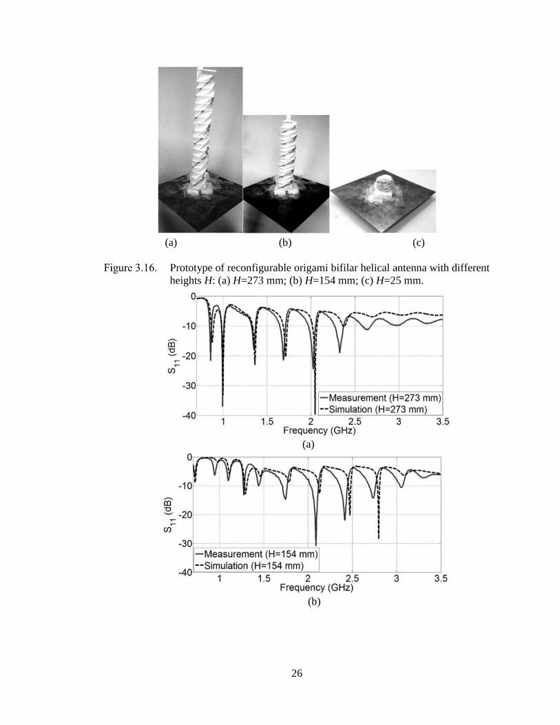
Figure 3.16 Prototype of reconfigurable origami bifilar helical antenna with

different heights H: (a) H=273 mm; (b) H=154 mm; (c) H=25 mm................26

Figure 3.17 Return loss of origami bifilar helix for different antenna heights, H...............27

Figure 3.18 Realized gain at zenith for three heights of the origami bifilar helix in

three different operating frequency bands......................................................28

Figure 3.19 Normalized elevation patterns of the origami bifilar helical antenna at

the operating frequencies of the three states (i.e., Heights): (a) H=273 mm

xiii

at 0.86 GHz; (b) H=154 mm at 1.27 GHz; (c) H=154 mm at 1.7 GHz;

(d) H=154 mm at 1.98 GHz; (e) H=25 mm at 2.49 GHz; (f) H=25 mm at

2.81 GHz; (g) H=25 mm at 3 GHz.................................................................30

Figure 3.20 (a) Origami helical tube and (b) Origami bellow tube.....................................32

Figure 3.21 Folding patterns of: (a) helical tube based QHA and (b) bellow tube

based QHA.....................................................................................................32

Figure 3.22 Geometry of one step of origami tube: (a) perspective view and

(b) top view....................................................................................................33

Figure 3.23 Simulation models of origami antennas based on: (a) helical tube; and

(b) bellow tube................................................................................................33

Figure 3.24 Simulated RHCP realized gain of QHA on helical tube..................................34

Figure 3.25 Simulated RHCP realized gain of QHA on bellow tube..................................35

Figure 3.26 Simulated AR of QHA on helical tube............................................................35

Figure 3.27 Simulated AR of QHA on bellow tube............................................................35

Figure 3.28 (a) Planar antenna layout, and (b) origami QHA on Kapton helical

tube................................................................................................................37

Figure 3.29 S11 results of QHA on helical tube at: (a) state 1, (b) state 2, (c) state 3

and (d) state 4................................................................................................38

Figure 3.30 RHCP gain of QHA on helical tube at: (a) state 1, (b) state 2, (c) state 3

and (d) state 4................................................................................................39

Figure 3.31 RHCP radiation patterns of QHA on helical tube at: (a) state 1 at

1.08 GHz, (b) state 2 at 1.56 GHz, (c) state 3 at 2.18 GHz and

(d) state 4 at 3.34 GHz...................................................................................39

Figure 4.1 Geometries of the origami multi-radii monofilar helix: (a) origami

folding pattern, (b) perspective view of multi-radii folded-up

transitional section, and (c) top view of multi-radii folded-up

transitional section..........................................................................................42

Figure 4.2 Model and geometries of the origami multi-radii monofilar helix at

three different heights (i.e., states): (a) state 1 (unfolded state), (b) state 2

(semi-folded state), and (c) state 3 (folded state) .............................................46

Figure 4.3 The geometries of: (a) standard helix, and (b) standard multi-radii helix..........50

Figure 4.4 Comparison of simulated S11 of standard monofilar, standard multi-radii,

and origami multi-radii helices........................................................................51

Figure 4.5 Comparison of simulated zenithal RHCP realized gain of standard,

xiv

standard multi-radii, and origami multi-radii helices.......................................51

Figure 4.6 Comparison of simulated zenithal axial ratio of standard,

standard multi-radii, and origami multi-radii helices.......................................51

Figure 4.7 Comparison of simulated radiation patterns of standard, Standard

multi-radii, and origami multi-radii helices at their center frequency

of operation, fc.................................................................................................52

Figure 4.8 The origami monofilar to be compared with the origami multi-radii

monofilar at: (a) state 1 (unfolded state), (b) state 2 (semi-folded state),

and (c) state 3 (folded state).............................................................................54

Figure 4.9 Comparison of simulated S11 of origami single-radius and multi-radii

helices at three states (blue lines: state 1; black lines: state 2; red lines:

state 3)............................................................................................................54

Figure 4.10 Comparison of simulated realized RHCP gain of origami single-radius

and multi-radii helices at three states (blue lines: state 1; black lines:

state 2; red lines: state 3).................................................................................55

Figure 4.11 Comparison of simulated axial ratio of origami single-radius and

multi-radii helices at three states (blue lines: state 1; black lines:

state 2; red lines: state 3)................................................................................55

Figure 4.12 Comparison of simulated elevational radiation patterns of the origami

single-radius and multi-radii helices at the center frequencies fc in their

2-dB realized gain bandwidths at: (a) state 1; (b) state 2; and (c) state 3........58

Figure 4.13 Models of multi-radii monofilar with variable fscale........................................59

Figure 4.14 Models of multi-radii helix with variable S.....................................................62

Figure 4.15 Models of multi-radii helix with variable S1...................................................63

Figure 4.16 Prototype of origami multi-radii helix at 3 reconfigurable states....................66

Figure 4.17 Actuation mechanism of the origami multi-radii helix....................................66

Figure 4.18 Simulated and measured S11 results of the origami multi-radii helix at:

(a) state 1, (b) state 2 and (c) state 3................................................................68

Figure 4.19 Simulated and measured realized RHCP gain of the origami multi-radii

helix at: (a) state 1, (b) state 2 and (c) state 3..................................................69

Figure 4.20 Simulated and measured axial ratio of the origami multi-radii helix at:

(a) state 1, (b) state 2 and (c) state 3................................................................70

Figure 4.21 Simulated and measured elevational radiation patterns of the origami

multi-radii helix at: (a) state 1 at 1.56 GHz, (b) state 2 at 3.16 GHz,

xv

and (c) state 3 at 3.88 GHz..............................................................................71

Figure 5.1 Origami folding pattern of the QHA cylinder base...........................................74

Figure 5.2 Origami quadrifilar helical antenna model........................................................74

Figure 5.3 The three states of the reconfigurable origami QHA with the foldable

reflector and the folding patterns of the reflector.............................................76

Figure 5.4 Simulated S11 of the reconfigurable origami QHA with the reflector at

three states.......................................................................................................76

Figure 5.5 Simulated realized RHCP gain of the reconfigurable origami QHA with the

reflector at three states.....................................................................................77

Figure 5.6 Simulated axial ratio of the reconfigurable origami QHA with the reflector

at three states...................................................................................................77

Figure 5.7 RHCP patterns at three states of the reconfigurable origami reflector QHA

at designated operating frequencies..................................................................78

Figure 5.8 RHCP patterns of reconfigurable QHA resonating at 3 designated

operating frequencies with one common reflector state...................................79

Figure 5.9 Geometry of the 10:1 scale model of the origami QHA. (a) origami

folding pattern, and (b) 3D model....................................................................80

Figure 5.10 Geometry of 10:1 scale model of the origami QHA with its reflector at

three states: (a) state 1 (H=120 mm); (b) state 2 (H=75 mm); (c) state 3

(H=105 mm)..................................................................................................80

Figure 5.11 Geometry of 10:1 scale model of the origami QHA with its reflector.............81

Figure 5.12 Comparison of simulated and measured S11 at the three states........................82

Figure 5.13 Simulated and measured normalized radiation patterns at the three states:

(a) state 1 at 2.07 GHz, (b) state 2 at 3 GHz, and (c) state 3 at 4.45 GHz........83

Figure 5.14 Geometry of single reflector element: (a) top view; and (b) side view............85

Figure 5.15 Antenna array model at: (a) state 1, (b) state 2 and (c) state 3..........................85

Figure 5.16 Fabricated prototype of the 7-element origami helical array...........................86

Figure 5.17 Simulated and measured radiation patterns of the helical array at (a) state

1 at 2.07 GHz, (b) state 2 at 3 GHz and (c) state 3 at 4.45 GHz........................86

Figure 6.1 (a) Kresling origami pattern, (b) Top view and perspective view of one

step of the pattern............................................................................................89

Figure 6.2 Model of the conical and planar spiral antenna.................................................90

xvi

Figure 6.3 Simulated realized gain at the two states...........................................................90

Figure 6.4 Radiation patterns at 2.7 GHz: (a) conical spiral; (b) planar spiral....................91

Figure 6.5 Front to back ratio at the two states...................................................................91

Figure 6.6 (a) The 4-step origami pattern of spherical helical antenna; and

(b) one folded step...........................................................................................92

Figure 6.7 The 4 states of the spherical antenna: (a) state1 (h=8.69 mm); (b) state 2

(h=21.8 mm); (c) state 3 (h=11.6 mm); and (d) state 4 (h=6.5 mm) .................93

Figure 6.8 The simulated S11 at the 4 states of height.........................................................93

Figure 6.9 Simulated radiation patterns of the 4 states at their resonant frequencies:

(a) h=28.6 mm at 2.32 GHz; (b) h=21.8 mm at 1.77 GHz; (c) h=11.6 mm

at 2.07 GHz; (d) h=6.5 mm at 2.12 GHz.........................................................94

1

CHAPTER 1

INTRODUCTION

1.1 Problem Statement

During the last twenty years, mathematicians and engineers have done extensive

research focusing on the mathematical basis of origami and reconfigurable systems [1]-[2].

Mathematical analysis of origami geometries were demonstrated by generations of origami

artists [3]-[5], and it took several years for origami scientists to solve the fundamental

problem of defining the folded state of an origami [6]. The issues the origami scientists and

engineers aim to solve are either paper folding, or the construction of a reconfigurable

object or a suitable mechanism to reconfigure it. The reconfiguration of an object serving

a certain purpose usually means folding and unfolding, and the property of an object being

able to unfold is often referred to as deployability, while its ability to fold is referred to as

stowability. Such reconfigurable objects can be stowed compactly to fit in a very small

volume and be deployed to occupy a larger volume. Therefore, they can have practical

applications in numerous scenarios, such as, a telescopic lens that has to fit into a small

compartment before it can be launched into orbit and then be unfolded into a large size to

operate [7], or a deployable heart stent that can travel through human blood vessel to an

optimum operational location where it will unfold in response to temperature to carry out

invasive heart surgery [8]. Also, origami has been applied on the design of automobile

airbags that deploy fast and are stowed compactly [9]. Different kinds of inflatable origami

cylindrical booms to pack or rigidize space structures have been introduced [10]. In

addition, origami has been used to make hollow cell structures for the next-generation

medical devices, e.g., stents that are more compatible to human body [11]. Furthermore,

2

self-folding robots have been proposed for rapid prototyping and self-assembly of devices

in space [12].

Various complex geometries have been used in electromagnetics to develop

components with enhanced performance and unique capabilities, such as fractal antennas

[14]. Dr. Tentzeris has also performed 3-D folding of antennas for various flexible and

wearable applications [25]. Dr. Georgakopoulos has worked on 2-D and 3-D folding of

Strongly Coupled Magnetic Resonance elements used to wirelessly power devices [26].

Limited previous work on origami electromagnetic structures has been performed by others

[20].

Also, to our knowledge no mathematical optimization of origami foldable antennas

has been performed and no methodologies that address the challenges of designing origami

foldable electromagnetic structures on paper, fabric and other flexible substrates have been

developed before our work.

1.2 Research Objectives and Contributions

The first aim of this research is to develop new deployable, collapsible, light-weight

and robust reconfigurable antennas based on origami. The designs will be validated through

simulations and measurements. Beyond paper, other substrates, such as, Kapton and fabric,

will be used to develop robust origami antennas and their mechanical performance will be

studied. The second aim of this research is to derive integrated analytical and simulation

models for designing optimal origami antennas for various applications, such as, satellite

and ground communications.

3

1.3 Methodology

Today’s complex antennas are typically designed using full-wave simulation

software, such as the ANSYS HFSS. However, there is no direct way to parameterize

models of complicated structures such as origami antennas, because the surfaces of such

antennas are not continuous curves due to the existence of creases (hills and valleys). Also,

development of purely analytical methods for origami structures with more than two

degrees of freedom (i.e., more than two dimensions are changing simultaneously) would

be extremely difficult to derive. In this research, parameterized models of origami antennas

and reflectors will be derived based on various origami designs to expedite the design and

optimization process. The reconfigurability of origami antennas will be examined for

different performance parameters, such as, reflection coefficient, radiation pattern, axial

ratio and realized gain. The designs will be validated using measurements conducted with

vector network analyzers and anechoic chambers.

Suitable substrates will be studied to build robust foldable origami antennas with

improved reliability compared to conventional paper substrate, such as fabric or DuPont

Kapton. Origami antennas will be designed and printed on such materials and their

electromagnetic and mechanical performance will be validated through simulations and

measurements.

1.4 Dissertation Outline

The background work will be discussed in chapter 2. New reconfigurable origami

helical antennas will be proposed in chapter 3 and their performance will be characterized

and validated using simulations and measurements. A tri-band multi-radii monofilar helix

4

with improved circular polarization will be developed and analyzed in chapter 4. A

quadrifilar helical origami antenna with a reconfigurable and an array of this antenna will

be discussed in chapter 5. Also, novel origami antennas such as origami kresling conical

spiral antennas and origami spherical helical antennas will be presented in chapter 6.

Finally, the conclusions or this work and future research will be discussed in chapter 7.

5

CHAPTER 2

BACKGROUND AND RELATED WORK

2.1 Origami Art

Origami is the art of paper folding. Origami is composed from two Japanese words:

oru which means folding, and kami which means paper. Art historians believe that

Japanese origami was invented sometimes in the centuries after Buddhist monks carried

paper to Japan during the 6th century [21]. Abstract folded paper forms were used in

religious ceremonies over many years, and by the 1600s, decorative shapes that we

recognize today (i.e., traditional crane) were being folded [22]. Modern origami art

emerged in 1950s and inspired a new generation of not only artists but also scientists. There

are two categories of origami: rigidly foldable origami, where stiff panels are folded along

hinged creases, which are geodesically fixed within the paper [23]; and non-rigidly-

foldable origami, where deformation is allowed on each individual face and/or vertices and

creases can move within the paper [24].

2.2 Reconfigurable Antennas

Antennas play a crucial role in communication systems since they are the

transmitting/receiving elements that transition information from guided transmission to

open-space propagation [13]. Antennas are used in many different applications such as

aerospace communications, mobile phones, TVs and radios. Since the dimensions of

antennas are usually physically proportional to the wavelength at their operating

frequencies, it is important to develop large antennas and arrays that can be stowed

compactly and easily deployed. Also, it is important to minimize the number of antennas

6

on a platform by developing multifunctional antennas. Various complex geometries have

been used in electromagnetics to, such as, fractal antenna [14]. A self-folding origami

antenna was proposed that can be converted from a patch antenna to a monopole antenna

in seconds, but this transition is not reversible [15]. Antennas with reflectors are preferred

in satellite communications for their high gain [16]-[17]. However, their large size and

heavy weight create significant problems, especially when these antennas need to be

carried by satellites into space. Compact foldable antennas have proposed using

conventional ways of fabrication [18]-[19], but they do not have the ability to reconfigure

their performance. Concepts of deployable antennas have been proposed in [20], but no

rigorous antenna models were developed.

7

CHAPTER 3

ORIGAMI HELICAL ANTENNA

3.1 Standard Axial Mode Helical Monofilar Antenna

Helical antennas have two principal modes: the normal (broadside) mode and the

axial (end-fire) mode. The axial mode has its maximum pattern along the axis of the helix.

This mode is usually the most practical because it can achieve circular polarization over a

wider bandwidth (usually 2:1) and it is more efficient [27]. The empirical optimum

parameters for an axial-mode circularly polarized monofilar helical antenna (geometry is

shown in Figure 3.1) are given in Table 3.1; where, S is the spacing between each turn and

C=πD is the circumference of the helix [27]-[28], and λ0 is the operational wavelength.

Also, the pitch angle, α, and the total length of conductive line, L, are given by Eqn. (3.1)

and (3.2) [27] below.

CStan (3.1)

2 2L N S C (3.2)

Geometry of standard helical antenna.

8

Table 3.1. Empirical Optimum Parameters of Monofilar Helical Antenna.

Parameter Optimum Range

Circumference 3λ0/4<C<4λ0/3

Spacing Between Each Turn Sλ0/4

Pitch Angle 12°<α<14°

Number of Turns 3<N

Ground Plane Diameter At least 0.5λ0

3.2 Analysis of Origami Helical Model

In this section, an analytical method is presented for designing an origami helical

antenna that mimics a standard helical antenna with specific defining parameters D, α, and

N. The folding pattern [29], which is used to fold the origami cylinder base of the helix, is

shown in Figure 3.2. The solid lines are hills and dashed lines are valleys. As illustrated in

Figure 3.2, the conductive (i.e., copper) lines are placed only along creases b, in order for

the origami helical antenna to achieve the maximum tunability of S. The number of

conductive lines can be 1, 2, or 4, and the total length of each conductive line is L.

The origami cylinder base of the helical antenna, as shown in Figure 3.3 (b), is

obtained by first folding the pattern of Figure 3.2 to obtain the geometry of Figure 3.3 (a),

and then connecting the left side of Figure 3.3 (a) to its right side from top to bottom. As

shown in Figure 3.4, the height of each step of the origami cylinder is defined as h and the

angle between each step and its adjacent step is defined as . Also, r is the distance from

the center of the polygon at the intersection to its furthest perimeter point, and is the

angle between two adjacent radial lines r.

The relationships between all the geometric parameters that define the origami

helical antenna are listed in Table 3.2, where ratio=b/a is the aspect ratio of each

parallelogram unit of the pattern in Figure 3.2, c is the length of the diagonal line in each

http://dict.youdao.com/w/parallelogram/

9

parallelogram unit and m is the total number of steps. Also, the minimum number of sides

n of a foldable pattern of the origami cylinder should be 3, as expressed in Eqn. (3.3). An

example of origami cylinder with the minimum n=3 is shown in Figure 3.5. Also, the ratio

should be properly chosen to achieve the desired antenna geometry and foldability

according to the analytical method that will be described below.

3,n n N (3.3)

Folding pattern of origami helix.

(a) (b)

Procedure of folding the origami cylinder substrate base. [29]

10

(a) (b)

Geometry of each step of the origami cylinder substrate base.

Origami cylinder with the minimum n=3.

For any given standard helical antenna, an equivalent origami helical antenna can

be derived when m and n are specified, and vice versa, as listed in Table 3.1. Specifically,

the standard helix and origami helix are equivalent in terms of the values of the spacing

between each turn S, pitch angle α, number of turns N, and total length L. Also, the

circumference of the standard helix is equal to the perimeter of the origami helix.

The empirical maximum gain of a numerically modeled standard helix can be

expressed as [27]

2

max 0 0( ) 10.25 1.22 / 0.0726 /G dB L L (3.4)

11

Table 3.2. Geometric Parameters of Origami Helical Antennas.

Parameters of Origami

Helix Relationships among Parameters

m, n, L, a, b, c, ratio,

β, γ, h, θ, r,

abratio n [32]

1sin sinration

,L m b m a ratio m N

2 2

2

2

sin2

sin

a

h b

n

2 n

2sin2

ar

2 sin sincos

1 cosc a ratio

Also, if we substitute in the Eqn. (3.4) L=mb and the approximation λ0=Cna

(where C is the circumference of the origami cylinder) to design an axial-mode origami

helix, which satisfies the conditions of Table 3.1, the empirical maximum gain of this axial-

mode origami monofilar helical antenna can be expressed as

2

max ( ) 10.25 1.22 0.0726m m

G dB ratio ration n

(3.5)

12

Table 3.3. Relationships between Standard and Origami Helices.

Standard Helix Relationships Equivalent Origami Helix

D, α, N

πa D n

2arcsin sinn

Nm n

sec sin( ) sin( )2

ration

m (given),

n (given),

a, θ, ratio

Origami Helix Relationships Equivalent Standard Helix

m, n, a, b, θ

2 2

2

2

sin

sin2

bn

S n a

2 2

2

( ) sin

tan 1

sin2

b

a n

sin sin2

N m nn

S, α, N

3.3 Comparison of Standard Helical Antennas with Equivalent Origami Helical

Antennas

An axial-mode standard helical monofilar antenna is designed and its parameters

are described in Table 3.4. The parameters of the equivalent origami helical monofilar

antennas are calculated according to Table 3.3 for different values of n or m, and are shown

in 0.

Table 3.4. Geometric Parameters of the Standard Helical Antenna.

D S tanα N

48 mm 37 mm 0.245 3

13

Table 3.5. Calculated Parameters of Equivalent Origami Helical Antennas with

Different Folding Patterns.

m=13 m=15 m=18

n=4

a=37.7 mm

ratio=0.95

θ=81.5°

a=37.7 mm

ratio=0.82

θ=68.9°

a=37.7 mm

ratio=0.69

θ=56.3°

n=4 n=5 n=6

m=13

a=37.7 mm

ratio=0.95

θ=81.5°

a=30.2 mm

ratio=1.19

θ=85.4°

a=25.1 mm

ratio=1.43

θ=87.6°

The simulated S11 of both the standard helical antenna and the equivalent origami

helical antennas are shown in Figure 3.6. The offset distances between these antennas and

their corresponding ground planes are kept the same, so are the radii of their circular ground

planes and the widths and thicknesses of their copper traces. All the models are excited

with 50 Ω SMA connectors. The simulated performances between the proposed standard

helical antenna and its equivalent origami helical antennas are listed in Table 3.6. In the 3-

dB gain bandwidths, the side lobes stay 10 dB lower than the main lobe for all the antennas.

14

(a)

(b)

Comparison of S11 of a standard helical monofilar antenna and its

equivalent origami helical monofilar antennas: (a) equivalent origami helix with n=4,

m=13, 15, 18; (b) equivalent origami helix with m=13, n=4, 5, 6.

The following conclusions can be drawn from Table 3.6:

1) The equivalent origami helical antennas can operate equally well to the

standard helical antenna in terms of maximum gain (<1 dB difference) and 3-dB gain

bandwidth (±2.6% difference).

2) The RHCP bandwidth of the standard antenna is 5.1%-10.8% larger than

that of the equivalent origami antennas.

15

3) A different m or n in the origami pattern will change the geometry of the

origami antenna, and a larger n improves the CP bandwidth because the n-side polygon at

the intersection of the origami helix has a geometry that resembles a circle more closely.

Table 3.6. Performance Comparison of Standard Helical Monofilar Antenna and Its

Equivalent Origami Helical Monofilar Antennas.

Antennas 3-dB Gain

Bandwidth

RHCP Bandwidth

(axial ratio<3 dB)

Maximum

Realized Gain

Standard Helix 1.75-3.3 GHz

(1.89:1)

1.78-3.3 GHz

(1.85:1) 12.87 dB

Origami

Helix

n=4

m=13

1.65-3.15 GHz

(1.91:1)

1.89-3.15 GHz

(1.67:1) 12.23 dB

n=4

m=15

1.7-3.2 GHz

(1.88:1)

1.87-3.2 GHz

(1.71:1) 12.29 dB

n=4

m=18

1.65-3.1 GHz

(1.88:1)

1.81-3.1 GHz

(1.71:1) 12.28 dB

Origami

Helix

n=4

m=13

1.65-3.15 GHz

(1.9:1)

1.89-3.15 GHz

(1.67:1) 12.23 dB

n=5

m=13

1.7-3.25 GHz

(1.91:1)

1.88-3.25 GHz

(1.73:1) 11.94 dB

n =6

m=13

1.7-3.3 GHz

(1.94:1)

1.88-3.3 GHz

(1.76:1) 12.08 dB

Based on Table 3.2, reconfigurable origami helical antennas that can operate at

various frequencies of interest can be parametrically modeled and designed. As an example,

a bifilar reconfigurable origami helical antenna is presented in 3.4. Furthermore, the

proposed origami helical antennas can be folded to fit in compact storage/launching

compartments thereby providing significant savings of volume for space-borne and

airborne applications, such as, satellites.

16

For an origami cylinder to be collapsible to a compact volume, then the diagonal

length, c, of one parallelogram unit in the origami pattern in Figure 3.2 should be less than

the diameter of the origami cylinder, 2r, in Figure 3.4 when the origami cylinder is

completed collapsed (h0). When a collapsible origami cylinder substrate is folded and

completely collapsed, the height of each layer h=4t where t is the thickness of the substrate,

so the total height of the collapsed origami cylinder structure is 4mt. On the other hand,

when the origami cylinder structure is fully deployed, it has a total height of mbsin(+).

Since the footprint of the origami cylinder structure can be expressed as 2 2

4

n a

, the

minimum and maximum volume of a collapsible origami cylinder are respectively

expressed as:

2 2

minπ

mtn aVolume (3.6)

2 2

max

sin( )

4π

mb n aVolume

(3.7)

To quantify the volume savings achieved by this collapsible origami cylinder when

it is stored, the compactness factor is defined as the ratio between the maximum and

minimum volume of a collapsible origami cylinder, and is expressed in Eqn. (3.8).

max

min

sin( )

4compact

Volume bF

Volume t

(3.8)

When cR+

and c<2r, by applying expressions of

and in Table 3.2, the

compactness factor depends only on the geometric parameters (n, a

and ratio)

defined in

Figure 3.2 and thickness t of the origami pattern, as shown in Eqn. (3.9).

17

1sin sin sin

4compact

a ratioF ratio

t n n

(3.9)

The plots of compactness factor versus each parameter for a collapsible origami

cylinder are shown in Figure 3.7. It is shown in Figure 3.7 (a)-(c) that Fcompact is

proportional to a and the ratio, and inversely proportional to t, regardless the values of all

other parameters. Also, Figure 3.7(c) shows that an optimum value of ratio exists for each

different n, which provides the maximum compactness factor, Fcompact. Also, when ratio is

fixed, an optimum n needs to be selected to achieve the maximum Fcompact. Furthermore,

when n increases, the maximum Fcompact also increases.

(a)

18

(b)

(c)

Compactness factor vs.: (a) the length, a, of each parallelogram unit in the

origami pattern; (b) thickness of substrate t (mm); (c) ratio of b/a with a=22.5 mm and

t=0.2 mm.

19

Using Table 3.1 and Table 3.3, and by applying 0

0

c

f , we can conclude that

the empirical operational frequency range of an origami monofilar helical antenna is:

0

3 4

4 3

c cf

na na (3.10)

or

2 2

2

02

sin

4

sin2

bn

f c n a

(3.11)

where c is the speed of light. Also, the proposed origami helical antenna can be designed

to achieve optimal gain at multiple frequencies in the frequency range of Eqn. 3.10 and

exhibit frequency reconfigurability by changing , as shown by Eqn. 3.11.

3.4 Reconfigurable Helical Antenna Based on Origami Neoprene with High

Radiation Efficiency

3.4.1 Antenna Geometry

This paper presents a novel way of building a reconfigurable helical antenna that

improves its mechanical robustness. The origami folding pattern of the cylindrical base is

shown in Figure 3.8 (a), where the conductive trace is placed along the diagonal lines in

the parallelogram unit to achieve more turns than along the side b. The folded antenna

based on the cylindrical origami substrate is shown in Figure 3.8 (b). The geometrical

parameters are listed in Table 3.7.

20

(a) (b)

Geometry of: (a) origami pattern, and (b) folded antenna.

Table 3.7. Values of Geometrical Parameters of the Antenna.

m n w a b h L

5 8 18 mm 40 mm 75 mm 5 mm 200 mm

(a) (b)

Model of one step: (a) perspective view, and (b) top view.

The total height H and number of turns N of the antenna are expressed below:

2

2 2

2

sin2

sin2

H m b a

(3.12)

( )

360

mN

(3.13)

where is the folding angle between adjacent step, and α is the inner angle between two

radial lines in the n-polygonal plane, as shown in Figure 3.9 (b).

21

3.4.2 Prototype of the Helical Antenna

Neoprene can withstand extreme temperature and weather and has exceptional

durability. Therefore, it is used here as the origami base for our antenna. The origami

folding pattern on the neoprene substrate can be generated by preheating the neoprene,

placing it inside a heated metal mold cavity and then applying pressure. A 0.1mm-thick

polyester fiber cloth coated with high conductive copper and nickel is used as the antenna

conductive trace to achieve abrasion and high temperature resistance, excellent flexibility

and conduction. This conductive cloth is sewn onto the 3-mm thick neoprene substrate

using conductive textile threads [30], as shown in Figure 3.10. At the unfolded state

H=310 mm and N=1.29; while at the folded state H=125 mm and N=1.8.

(a) (b)

Prototype of the helical antenna on Neoprene at: (a) unfolded state, and (b)

folded state.

3.4.3 Simulated and Measured Results

The antenna was simulated in ANSYS HFSS and measured with Agilent VNA and

StarLab Anechoic Chamber. The simulated and measured S11 is shown in Figure 3.11. It

22

can be seen that the simulated resonant frequencies are higher than the measured ones,

which is because of the effect of the neoprene substrate, which is not included in simulation.

Simulated and measured S11 at unfolded and folded states.

The simulated and measured realized gain and AR are compared in Figure 3.12-

Figure 3.13, and the measured results are summarized in Table 3.8. It is verified that the

helical antenna on neoprene radiates directionally at the two states and achieves

reconfigurable frequency in wide bandwidth with maximum gain of at least 9.2 dB at the

two states. Also, the prototype fabricated with conductive polyester on neoprene substrate

has very good radiation efficiency, which is greater than 80%, as shown in Figure 3.14.

Furthermore, this antenna exhibits improved robustness compared to origami antennas

made on flexible substrates, such as, paper and Kapton. Therefore, this antenna is a good

candidate for real-world applications as it can easily deploy/collapse and reconfigure its

performance while maintaining it mechanical performance through a large number of

folding/unfolding cycles without experiencing cracking of the substrate or the conductive

trace.

23

Simulated and measured realized gain at unfolded and folded states.

Simulated and measured AR at unfolded and folded states.

Measured radiation efficiency at unfolded and folded states.

24

Table 3.8. Summarized Measured Results of The Antenna.

3.5 Reconfigurable Origami Bifilar Helical Antenna

Here, an example of an origami bifilar antenna is shown in Figure 3.15. One helix

is connected to the signal excitation (center conductor of SMA) and another identical helix

is grounded for more symmetric radiation patterns especially at lower resonant frequencies.

Moreover, the grounded helix enables the bifilar helical antenna to operate in axial mode

at its lowest resonant frequency, which occurs when it is fully deployed (i.e., helix is

deployed to its maximum height).

Origami bifilar helical antenna model at different states of H.

The height of the antenna can vary as the origami structure can collapse and expand.

The total height of this antenna is H=m·h. The number of steps m=18, the number of sides

n=6, the side length of each parallelogram unit in the pattern a=22.5 mm, and the ratio=1.

Max. Realized Gain 3-dB Realized Gain BW CP BW (AR<3 dB)

Unfolded State 9.4 dB 1.56 GHz-3.04 GHz (64.3%) 2.57 GHz-2.8 GHz (8.6%)

Folded State 9.2 dB 0.8 GHz-1.78 GHz (76%) 1.04 GHz-1.28 GHz (20.7%)

25

The side length of the square ground is 200 mm. A polyethylene base (εr=1.2) is placed

between the antenna and the ground in the prototype to provide a physical support for the

antenna and prevent it from being shorted. The prototype of the origami bifilar is shown in

Figure 3.16. This antenna was constructed using 0.1 mm thick copper tape on 0.2 mm thick

sketching-paper substrate without any coating. The height, H, of the prototype antenna is

controlled by applying a force at its top face.

The compactness factor of this reconfigurable bifilar helical antenna according to

Eqn. 12.9 is 24.36. Figure 3.7 (c) shows that for n=6, the optimum compactness factor of

47.79 is achieved when ratio=1.7. While for ratio=1, the optimum compactness factor of

26.75 is achieved when n=5.

The simulated and measured S11 for three different heights H, is illustrated in Figure

3.17. The simulated and measured realized gains at zenith for the fully unfolded state

(H=273 mm), the semi-folded state (H=154 mm) and the fully folded state (H=25 mm) in

different operating frequency bands are illustrated in Figure 3.18. The operating

frequencies of each state are depicted with solid triangles in Figure 3.18. The measured

results validate that this collapsible reconfigurable origami bifilar helical antenna can

operate at different frequencies by changing its height.

26

(a) (b) (c)

Prototype of reconfigurable origami bifilar helical antenna with different

heights H: (a) H=273 mm; (b) H=154 mm; (c) H=25 mm.

(a)

(b)

27

(c)

Return loss of origami bifilar helix for different antenna heights, H.

The differences between simulated and measured results occurring in Figure 3.17

and Figure 3.18 can be attributed to the fact that the prototype was constructed manually.

(a)

28

(b)

(c)

Realized gain at zenith for three heights of the origami bifilar helix in

three different operating frequency bands.

It should be also noted that this origami bifilar helical antenna is designed to operate

in axial mode at all the indicated operating frequencies of the three states (i.e., heights).

Table 3.9 shows that each state exhibits a higher gain at its own operating frequencies than

the gains of the other two states at these frequencies.

Table 3.10 illustrates the measured performances of the origami antenna for three

different antenna heights. Measured AR validated that this antenna is circularly polarized

(AR<2 dB) at 1.27 GHz, 1.7 GHz and 1.98 GHz when H=154 mm, while at the other two

29

states when H=273 mm and H=25 mm, this antenna operates with either linear or elliptical

polarization.

The normalized elevation-plane patterns are shown in Figure 3.19 at the operating

frequencies of each state. Figure 3.19 illustrates that this origami bifilar helical antenna

operates in axial mode at all the listed operating frequencies above with maximum gain at

zenith. It is seen that at higher operating frequencies the back lobes become smaller, which

is expected since at higher frequencies the ground plane is electrically larger.

Table 3.9. Measured Realized Gain (dB) at the Operating Frequencies of the 3 States

of the Origami Bifilar Helix.

Antenna Height H

(mm)

Frequency (GHz)

0.86 1.27 1.7 1.98 2.49 2.81 3

273 5.85 1.80 -0.58 -2.06 -2.11 -5.54 -2.00

154 -18.35 6.53 6.79 4.69 -0.13 -0.69 1.62

25 -19.73 -9.63 -8.7 -1.18 5.98 5.81 5.70

(a) (b) (c)

30

(d) (e)

(f) (g)

Normalized elevation patterns of the origami bifilar helical antenna at the

operating frequencies of the three states (i.e., Heights): (a) H=273 mm at 0.86 GHz; (b)

H=154 mm at 1.27 GHz; (c) H=154 mm at 1.7 GHz; (d) H=154 mm at 1.98 GHz; (e)

H=25 mm at 2.49 GHz; (f) H=25 mm at 2.81 GHz; (g) H=25 mm at 3 GHz.

Table 3.10. Measured Performances of the Bifilar Helical Origami Antenna for

Three Different Heights.

Antenna Height H (mm)

273 154 25

Operating Frequency (GHz) 0.86 1.27 1.7 1.98 2.49 2.81 3

Measured Realized Gain

(dB) 5.85 6.53 6.79 4.69 5.98 5.81 5.7

Measured E-Plane BW (°) 82 59 45 44 61 44 41

Measured H-Plane BW (°) 75 50 44 40 57 46 40

Measured AR (dB) 19.2 0.56 0.24 0.55 5.78 3.21 2.23

31

3.6 Frequency Reconfigurable QHA Based on Kapton Origami Helical Tube for

GPS, Radio and Wimax Applications

3.6.1 Analysis of origami structures of QHA

The origami helical tube was firstly proposed by Guest and Pellegrino [31] as

shown in Figure 3.20 (a). Origami bellow tube is a mutation of the origami helical tube by

simply rotating each adjacent step in different directions, as shown in Figure 3.20 (b). Here,

we propose new QHAs that are based on a 4-sided origami helical tube and an 8-sided

origami bellow tube. The folding patterns for these antennas are shown in Figure 3.21.

Solid lines are hills and dashed lines are valleys, and the orange parts denote the antenna

copper traces. The detailed geometry of one step of a helical or bellow tube is shown in

Figure 3.22. If the coordinates of point A in the parallelogram unit is (a, 0, 0), then the

coordinates of points B, C and D are calculated as shown in Figure 3.22 (a), where

α=360°/n is the inner angle of the polygon at the intersection of the origami tube. Also, la,

lb and lc can be calculated by the coordinates of their endpoints. Figure 3.22 (b) shows the

relative rotation angle θ between the top and bottom of each step. If we define ratio= lb /

la, then lc / la can be expressed as:

2 21 2cos( ) 4sin2

c

a

lratio

l

(3.14)

where the ratios in helical and bellow tubes are respectively 0.7 and 0.45, and la of helical

and bellow tubes are respectively 30 mm and 16.6 mm. Also, the height of each step

increases as folding angle θ decreases. The linear elastic strain can be analyzed as

32

201( )

2

c c

c

l lWw

E l

[32]. In this case, as θ decreases, the strain of both tubes increases, so

there is a maximum height both structures can achieve.

(a) (b)

(a) Origami helical tube and (b) Origami bellow tube.

(a)

(b)

Folding patterns of: (a) helical tube based QHA and (b) bellow tube based

QHA.

33

(a) (b)

Geometry of one step of origami tube: (a) perspective view and (b) top

view.

3.6.2 Helical and Bellow origami tube QHAs

Through analytical methods, models of helical and bellow origami tube QHAs are

parametrically modeled and simulated with HFSS. Examples of these simulation models

are shown in Figure 3.23, where N is the total number of turns, and pitch is the axial length

of each turn. They both are fed with four 50 Ohm-ports with a phase difference of 90

between adjacent ports. By increasing the folding angle θ, the height of each step, h, pitch

and the total height of antenna H decrease so that the antenna can operate at designated

frequency bands. The helical tube can be reconfigured by applying a rotating force at the

top of the helix, while the bellow tube can be reconfigured by an axial force only.

(a) (b)

Simulation models of origami antennas based on: (a) helical tube; (b)

bellow tube.

34

The simulated realized RHCP gain and axial ratio of the QHA on helical and bellow

tubes are shown in Figure 3.24-Figure 3.27. Shaded blocks denote their ±1 dB gain

bandwidth of each state. It can be seen that the QHA on the bellow tube only needs two

states to cover the GPS, radio and WiMax bands from 1.17 GHz to 3.5 GHz, because its

unfolded state has a higher gain than the helical tube based QHA at higher frequencies, i.e.

3-4 GHz. This happens because as the tube is unfolding the number of turns N (N=m/n) of

the bellow-tube QHA stays the same, whereas the number of turns N of the helical-tube

QHA decreases, as shown below:

180sin sin

2

N m n

n (3.15)

The performance of the QHAs on the two origami tubes are compared in Table 3.11.

Simulated RHCP realized gain of QHA on helical tube.

35

Simulated RHCP realized gain of QHA on bellow tube.

Simulated AR of QHA on helical tube.

Simulated AR of QHA on bellow tube.

36

Table 3.11. Performance Comparison of QHAs on Helical Tube and Bellow

Tube.

3.6.3 Prototypes and Results of Helical Tube Based QHA

The helical-tube QHA was built with copper traces sandwiched by Kapton substrate

for fabrication convenience since there are less creases in its folding pattern. The overall

thickness of the Kapton substrate is approximately 4 mils. The planar antenna layout is

shown in Figure 3.28 (a). The folded-up 3-D origami QHA is shown in Figure 3.28 (b). It

is centered at the square ground with 250 mm side-length which is fabricated with copper

foil glued on the back side of the black cardboard. The left and right sides of the substrate

are soldered together to build a robust cylinder. The 3-D printed cubic support beneath the

cylinder is 20 mm × 20 mm × 10 mm.

37

(a) (b)

(a) Planar antenna layout, and (b) origami QHA on Kapton helical tube.

Measurements were carried out with an Agilent VNA and a StarLab Anechoic

Chamber. The ports of the antenna are fed with 0, -90, -180 and -270 in a right-handed

order. Measured and simulated S11 results are compared in Figure 3.30.

The comparison of the simulated and measured RHCP gain at the four

reconfigurable states is depicted in Figure 3.31. It is seen that that the peak gain shifts to

higher frequencies as the antenna height, H, decreases. Also, at higher frequencies the

disagreement between measurements and simulations is bigger than the one at lower

frequencies. This is due to the fact that the Kapton substrate is not included in the

simulation models and at higher frequencies the effects of the Kapton substrate are more

pronounced. There is also a maximum 2-dB gain difference between simulated and

measured peak gains. This is mostly attributed to the insertion loss of the quadrature

feeding network. Typical operational frequencies of the 4 states are marked with triangles

on measured gain curves. Simulated and measured RHCP radiation patterns are compared

at the typical operational frequencies of the 4 states in Figure 3.31. The measured results

are summarized in Table 3.12 with the radiation pattern at the optimum gain points.

38

(a)

(b)

(c)

(d)

S11 results of QHA on helical tube at: (a) state 1, (b) state 2, (c) state 3 and

(d) state 4.

39

(a) (b)

(c) (d)

RHCP gain of QHA on helical tube at: (a) state 1, (b) state 2, (c) state 3

and (d) state 4.

(a) (b) (c) (d)

RHCP radiation patterns of QHA on helical tube at: (a) state 1 at

1.08 GHz, (b) state 2 at 1.56 GHz, (c) state 3 at 2.18 GHz and (d) state 4 at 3.34 GHz.

40

Table 3.12. Summarized Measured Results of Kapton QHA.

3.6.4 Conclusion

QHAs on origami helical tubes and bellow tubes were proposed in this chapter. The

bellow-tube QHA has wide bandwidth and it can reconfigure its height more easily by only

an axial force. On the other hand, the helical tube QHA has smaller number of creases and

it is easier to fabricate. The prototype of the helical-tube QHA was fabricated on Kapton

substrate, and its measured results show that it can successfully operate in RHCP axial

mode at reconfigurable states to cover GPS band in 1.17 GHz-1.58 GHz, satellite radio

band in 2.305 GHz-2.325 GHz and WiMax frequency at 3.5 GHz.

41

CHAPTER 4

A RECONFIGURABLE PACKABLE AND MULTIBAND ORIGAMI MULTI-RADII

HELICAL ANTENNA

Quasi-tapered helical antenna with multiple radii has been proved to have improved

gain, pattern, bandwidth and circular-polarization performances than conventional

uniform-diameter helical antennas [36]. Also, an analytical method to design origami

monofilar helices with a uniform diameter has been proposed in the last chapter. Despite

its frequency reconfigurability, this origami monofilar is only primarily circularly

polarized at the semi-folded state. In this chapter, we propose an origami multi-radii

monofilar helix with simple feed that operates in reconfigurable bandwidths with CP at

three states.

The proposed reconfigurable origami multi-radii monofilar helix exhibits improved

bandwidth, gain, pattern, and CP performance compared to those of the uniform-radius

standard monofilar or origami monofilar helices. The geometrical details of the multi-radii

origami base for the proposed antenna are demonstrated in § 4.1. The geometrical details

of the origami multi-radii helical antenna and the design process for this antenna are

discussed in § 4.2. The performance of this antenna is analyzed in § 4.3 and § 4.4. Also, an

actuation mechanism for this collapsible antenna is proposed in § 4.5. The performance of

this antenna at three reconfigurable states is validated through simulations and

measurements in § 4.6.

4.1 Geometries of Origami Base

The proposed origami multi-radii helix consists of two helical sections (a top and a

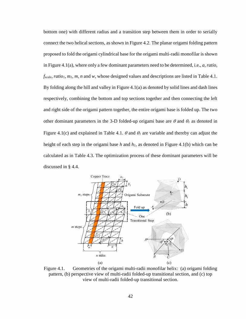
42

bottom one) with different radius and a transition step between them in order to serially

connect the two helical sections, as shown in Figure 4.2. The planar origami folding pattern

proposed to fold the origami cylindrical base for the origami multi-radii monofilar is shown

in Figure 4.1(a), where only a few dominant parameters need to be determined, i.e., a, ratio,

fscale, ratio1, m1, m, n and w, whose designed values and descriptions are listed in Table 4.1.

By folding along the hill and valley in Figure 4.1(a) as denoted by solid lines and dash lines

respectively, combining the bottom and top sections together and then connecting the left

and right side of the origami pattern together, the entire origami base is folded up. The two

other dominant parameters in the 3-D folded-up origami base are and 1 as denoted in

Figure 4.1(c) and explained in Table 4.1. and 1 are variable and thereby can adjust the

height of each step in the origami base h and h1, as denoted in Figure 4.1(b) which can be

calculated as in Table 4.3. The optimization process of these dominant parameters will be

discussed in § 4.4.

Figure 4.1. Geometries of the origami multi-radii monofilar helix: (a) origami folding

pattern, (b) perspective view of multi-radii folded-up transitional section, and (c) top

view of multi-radii folded-up transitional section.

43

Table 4.1. Primary Geometric Parameters of Origami Base.

Primary

Parameter Description

Designed

Value

n # of sides of the intersectional polygon 4

a Horizontal length of each parallelogram unit in the bottom

cylinder 35.4 mm

ratio Length ratio between the vertical and horizontal lengths of

each parallelogram unit in the bottom cylinder 0.7

m # of steps of the bottom monofilar 18

fscale Ratio of the radius of the top helix to the radius of the

bottom helix 0.8

ratio1 Length ratio between the vertical and horizontal lengths of

each parallelogram unit in the top cylinder 0.79

m1 # of steps of the top monofilar 18

w Width of the copper trace 15 mm

Folding angle between adjacent intersectional polygonal

planes in the bottom cylinder

Not

const.

1 Folding angle between adjacent intersectional polygonal

planes in the top cylinder

Not

const.

The relationships between the primary and the secondary geometrical parameters

of our antenna are shown in Table 4.2. These secondary parameters are necessary to model,

simulate and fabricate the proposed origami antenna accurately.

It can be seen from Table 4.2 that the lengths of diagonal lines (i.e., c, c1 and c0) in

this origami pattern and the side length b0 of the transitional step in Figure 4.1 (a) are not

constant due to the varying and 1. Therefore, the substrate applied to build the origami

base should be stretchable along these hinges besides being foldable; also, internal strains

will exist near these hinges. Angles in the transitional step (i.e., 0 and 0) denoted in Figure

4.1 (a) are also not constant due to its non-constant side lengths, so this origami pattern is

non-rigidly foldable, especially for the transitional step.

44

Table 4.2. Secondary geometric Parameters of Origami base.

Secondary

Parameters Calculation Value

2 n 90°

n [32] 45°

1sin sinratio [29] 29.7°

b ·b ratio a [29] 24.8 mm

c 2 sin sin

cos1 cos

c a ratio

Not

const.

b0 2

1 12 2

0

cos 0.5 cos 0.5

1 cos

scale scale

scale

f fb a f ratio

Not

const.

c0

2

1 12 2

0

cos 0.5 0.5 cos( ) 0.5

1 cos

scale scale

scale

f fc a f ratio

Not

const.

0

2 2 21 0 0 1

0

0 0

cos2

b c a

b c

Not

const.

0

2 2 21 0 0

0

0

cos2

c a b

ac

Not

const.

1 1

1sin sinratio 34°

a1 1 ·scalea f a 28.3 mm

b1 1 1 1·b ratio a 22.4 mm

c1 2 1

1 1 1

sin sincos

1 cosc a ratio

Not

const.

h

2

2

2

sin2

sinh a ratio

[29]

Not

const.

h1

2 1

2

1 1 1 2

sin2

sinh a ratio

Not

const.

4.2 Geometries of Antenna Model

The proposed reconfigurable multi-radii origami helix at 3 reconfigurable states of

height is shown in Figure 4.2. The pitch sizes of the bottom and top helices S and S1 can be

solely determined by ratio and ratio1, respectively, as shown in Eqn. (4.1) and (4.2). Also,

45

the number of turns of the bottom and top helices, N and N1 can be optimized independently

solely by changing m1 and m, respectively, without changing the values of the other

primary geometric parameters, as expressed below in Eqn. (4.3) and (4.4) [29]:

2 2

2

sin2

1

sin2

ratio

S n a

(4.1)

2 2

1

12 1

sin2

1

sin2

scale

ratio

S na f

(4.2)

sin sin2 2

N m n

(4.3)

11 1 sin sin

2 2N m n

(4.4)

Note that the number of turns N0 and height h1 of the transitional step do not

significantly impact performance of the antenna, and N0 is calculated as:

10 sin sin

2 2N n

(4.5)

Therefore, the geometries of the two helices can be optimized in terms of axial

ratio (AR) and 2-dB RHCP realized gain bandwidth by varying the geometric parameters

of the origami pattern (i.e., ratio, ratio1, m and m1). The designing process for this antenna

will be detailed in Section 4.4. The circumferences of both the bottom and top helices, C

and C1, remain approximately constant for different heights (i.e., states of the antenna), as

shown in Figure 4.2. Also, the total length of the antenna trace Ltotal=mb+b0+m1b1 remains

approximately constant at the 3 states.

46

(a) (b) (c)

Figure 4.2. Model and geometries of the origami multi-radii monofilar helix at three

different heights (i.e., states): (a) state 1 (unfolded state), (b) state 2 (semi-folded state),

and (c) state 3 (folded state).

According to antenna theory [37] and previous analysis on axial-mode origami

helical antenna [29]. The pitch size S, circumference C and pitch angle α of a broadband

single-radius origami helical antenna should satisfy the following conditions in order to

achieve optimal performance:

0 / 4S (4.6)

0 0

3 4

4 3C (4.7)

12 14 (4.8)

where,

2 2

1 1

2 22

sin2

tan tan 1

sin2

ratioh

b h

(4.9)

Also, the sense of the circular polarization is determined by the winding direction

of the helical trace from its feeding point. The proposed multi-radii origami helix is

47

designed to be right-hand circularly polarized (RHCP).

It can be concluded from Eqn. (4.7) that our origami helix can operate in axial mode

and have the following bandwidth:

0

3 4

4 3

c cf

na na (4.10)

Also, the length of one turn of the axial-mode CP helical antenna should be:

2 2

0L S C (4.11)

At lower frequencies than the ones covered by Eqn. (4.10), when λ0>>L, a helical

antenna operates in normal mode; while at higher frequencies, when λ0<<L, a helical

antenna operates in conical mode. Our origami helical antenna is collapsible and therefore,

it can vary its height, which in turn changes L. The length of one turn L can be written as a

function of , using L=Ltotal/N, where N depends on as shown in Eqn. (4.3). As L changes

for different heights, our origami helix can be made to operate in axial-mode at different

frequency bands, (i.e., exhibit multi-band operation). Specifically, if L increases, the

operating frequency band decreases and vice versa.

However, if we used a single-radius origami helix, then α, S and C shown in Eqns.

(4.6)-(4.8) would be out of the optimal CP range when the antenna operates at states 1 & 3

as shown in Figure 4.8, which would cause the gain and bandwidth of the antenna to

decrease at both states, and the polarization not to be CP at state 3.

Therefore, to address this problem and to improve RHCP gain, radiation pattern, 2-

dB realized RHCP gain bandwidth or CP performance at all three states of operation, a

second helix with different radius is added on top of the single helix [36]. The geometric

details of the proposed multi-radii origami helix are shown in Table 4.1 Table 4.2 and

Figure 4.2.

48

Here, we summarize the performance trends that were derived by our simulation

analysis (see § 4.4 for supportive data). When the circumference of the top helix, C1,

increases while staying smaller than C, the RHCP gain and AR are improved without

impacting the 2-dB RHCP realized gain bandwidth. However, when C1 increases beyond

C, the RHCP gain stops increasing, and the bandwidth and AR worsen. When the number

of turns of either the bottom or the top helix increases, the RHCP realized gain increases

inside its 2-dB RHCP realized gain bandwidth, while the RHCP gain bandwidth first

increases and then decreases. When the pitch size of the top helix, S1, increases, the 2-dB

RHCP realized gain bandwidth first increases and then decreases without significantly

affecting the RHCP realized gain, and AR tends to improve. Adding a third smaller helical

section on top of the multi-radii helix in Figure 4.2 does not improve bandwidth according

to our simulated results. Therefore, the results of an antenna that is composed by three

helices are omitted.

Based on these findings, the design process of a multi-radii helix is as follows:

1) a proper circumference of the bottom helix, C, is chosen for the desired

operating frequency band;

2) a proper circumference of the top helix, C1, is chosen to improve AR and

RHCP gain in the designed frequency band;

3) the proper number of turns of the bottom helix is chosen to optimize the 2-

dB RHCP realized gain bandwidth;

4) the number of turns of the top helix is chosen to achieve a compromise

between 2-dB RHCP realized gain bandwidth and the maximum zenithal RHCP gain;

5) the pitch size of the bottom helix, S, is optimized to achieve multiband

49

operation;

6) pitch size of the top helix, S1, is optimized for each reconfigurable state to

improve their 2-dB RHCP realized gain bandwidth and CP performance.

4.3 Comparison of Origami Multi-Radii Monofilar with Standard and Origami

Helices

4.3.1 Comparison of Origami Multi-Radii Monofilar with Standard Helix

The performance of the semi-folded state of the origami multi-radii helix, shown in

Figure 4.2(b), is compared with the performance of a standard helix and a standard multi-

radii helix, shown in Figure 4.3. The pitch sizes, circumferences, and pitch angles of the

standard multi-radii helix are the same with the ones of the proposed origami multi-radii

helix in Figure 4.2(b). The geometric parameters of the standard helix are the same with

the ones of the bottom helix in the origami multi-radii antenna in Figure 4.2(b). Also, all

three antennas have the same uniform copper width of 15 mm and a total number of turns

of approximately 6.3. All other geometric parameters are also kept the same, including

ground plane sizes (D=200 mm), distances from the ground (3.5 mm), SMA feeding ports

and positions of the antennas for a fair comparison. The pitch angle for all three antennas,

α, are 12.5° which fall into the optimum range (12° to 14°) to achieve optimal circular

polarization [29].

Figure 4.4-Figure 4.7 compare the performance (i.e., reflection coefficient, zenithal

realized RHCP gain, zenithal AR and radiation patterns) of the three antennas. Also, Table

4.3 summarizes the performance of the three antennas and the best performance out of the

three is shaded for each performance metric. The simulation analysis was performed by

50

ANSYS HFSS. The fractional bandwidth Δf is calculated as [37]:

max min

max min

100%2

f ff

f f

(12)

(a) (b)

Figure 4.3. The geometries of: (a) standard helix, and (b) standard multi-radii helix.

It can be concluded from these results that:

1) The origami multi-radii helix exhibits widest S11 bandwidth, as shown in

Figure 4.4.

2) The standard multi-radii helix has the largest RHCP realized gain but has

the narrowest 2-dB RHCP realized gain bandwidth (Δf=35.9%).

3) Our origami multi-radii helix has the widest 2-dB RHCP realized gain

bandwidth (Δf=66.2%), which is approximately two times larger than the one of the

standard multi-radii helix, while its maximum RHCP realized gain is smaller than the one

of the standard multi-radii helix only by 1.1 dB, as shown in Figure 4.5.

4) Our origami multi-radii helix has the widest CP bandwidth with AR<3 dB

and the best AR performance (i.e., AR<0.7 dB) during 2-dB RHCP gain BW out of all the

three antennas compared here, as shown in Figure 4.6.

51

5) The origami multi-radii helix also exhibits reconfigurable operating

frequency band by changing its height as demonstrated in Section 4.2, whereas the two

standard helical antennas do not.

Figure 4.4. Comparison of simulated S11 of standard monofilar, standard multi-radii,

and origami multi-radii helices.

Figure 4.5. Comparison of simulated zenithal RHCP realized gain of standard,

standard multi-radii, and origami multi-radii helices.

Figure 4.6. Comparison of simulated zenithal axial ratio of standard, standard multi-

radii, and origami multi-radii helices.

Also, the elevational radiation patterns of the three antennas at their corresponding

center frequencies of operation, fc=(fmax+fmin)/2, are compared in Figure 4.7. Square ground

52

planes of the same electrical size (D=1.5λc) at their fc were used for fair comparison of their

sidelobes. It can be seen from Figure 4.7 that the multi-radii helices (origami and standard)

have lower sidelobes than the ones of the standard helix.

Therefore, compared to the standard helices, the proposed origami multi-radii helix

exhibits a larger S11 bandwidth by up to 2%, a larger CP BW by up to 22%, a larger 2-dB

RHCP realized gain bandwidth by up to 30.3% and the smallest AR. These outweigh the

fact that the origami multi-radii helix exhibits a smaller RHCP gain by 1.1 dB compared

to the standard multi-radii helix. In fact, the gain of the origami multi-radii helix can be

further enhanced by adding a reflector without impairing its CP performance.

(a) (b)

Figure 4.7. Comparison of simulated radiation patterns of standard, standard multi-

radii, and origami multi-radii helices at their center frequency of operation, fc.

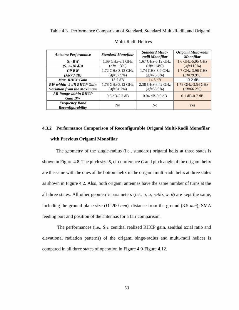
53

Table 4.3. Performance Comparison of Standard, Standard Multi-Radii, and Origami

Multi-Radii Helices.

Antenna Performance Standard Monofilar Standard Multi-

radii Monofilar

Origami Multi-radii

Monofilar

S11 BW

(S11<-10 dB)

1.69 GHz-6.1 GHz

(Δf=113%)

1.67 GHz-6.12 GHz

(Δf=114%)

1.6 GHz-5.95 GHz

(Δf=115%)

CP BW

(AR<3 dB)

1.72 GHz-3.12 GHz

(Δf=57.9%)

1.74 GHz-3.9 GHz

(Δf=76.6%)

1.7 GHz-3.96 GHz

(Δf=79.9%)

Max. RHCP Gain 13.7 dB 14.3 dB 13.2 dB

BW within -2 dB RHCP Gain

Variation from the Maximum

1.78 GHz-3.12 GHz

(Δf=54.7%)

2.38 GHz-3.42 GHz

(Δf=35.9%)

1.78 GHz-3.54 GHz

(Δf=66.2%)

AR Range within RHCP

Gain BW 0.6 dB-2.3 dB 0.04 dB-0.9 dB 0.1 dB-0.7 dB

Frequency Band

Reconfigurability No No Yes

4.3.2 Performance Comparison of Reconfigurable Origami Multi-Radii Monofilar

with Previous Origami Monofilar

The geometry of the single-radius (i.e., standard) origami helix at three states is

shown in Figure 4.8. The pitch size S, circumference C and pitch angle of the origami helix

are the same with the ones of the bottom helix in the origami multi-radii helix at three states

as shown in Figure 4.2. Also, both origami antennas have the same number of turns at the

all three states. All other geometric parameters (i.e., n, a, ratio, w, ) are kept the same,

including the ground plane size (D=200 mm), distance from the ground (3.5 mm), SMA

feeding port and position of the antennas for a fair comparison.

The performances (i.e., S11, zenithal realized RHCP gain, zenithal axial ratio and

elevational radiation patterns) of the origami singe-radius and multi-radii helices is

compared in all three states of operation in Figure 4.9-Figure 4.12.

54

(a) (b) (c)

Figure 4.8. The origami monofilar to be compared with the origami multi-radii

monofilar at: (a) state 1 (unfolded state), (b) state 2 (semi-folded state), and (c) state 3

(folded state).

Figure 4.9. Comparison of simulated S11 of origami single-radius and multi-radii

helices at three states (blue lines: state 1; black lines: state 2; red lines: state 3).

55

Figure 4.10. Comparison of simulated realized RHCP gain of origami single-radius and

multi-radii helices at three states (blue lines: state 1; black lines: state 2; red lines: state 3).

Figure 4.11. Comparison of simulated axial ratio of origami single-radius and multi-

radii helices at three states (blue lines: state 1; black lines: state 2; red lines: state 3).

The comparison of these results is summarized in Table 4.4. The following

conclusions are drawn:

1) The standard origami helix, shown in Figure 4.8, can operate in only the

first two states with CP performance covering the following frequency band: 1.3 GHz-3.46

GHz. However, the proposed origami multi-radii helix can operate at three states with CP

performance covering the following bands: 1.22 GHz-3.54 GHz and 3.64 GHz-4.04 GHz.

56

2) The origami multi-radii helix has a smaller maximum AR at states 2 and 3,

as shown in Figure 4.11.

3) At states 2 and 3, the origami multi-radii helix has lower sidelobe level than

that of the standard origami helix. Also, at state 3 the origami multi-radii helix has a

maximum RHCP gain that is larger by 2.8 dB than the one of the standard origami helix.

Table 4.4. Performance Comparison of Origami Multi-Radii Monofilar with Origami

Monofilar.

State of Origami

Antennas

S11 BW

(S11<-10 dB)

CP BW

(AR<-3 dB)

Realized RHCP

Gain BW

within -2 dB

Variation from

the Maximum

Max.

Realized

RHCP

Gain

AR Range

within 2-

dB RHCP

Gain BW

1

Origami

Monofilar

1.56 GHz-

5.96 GHz

(Δf=117%)

1.32 GHz-

4.2 GHz

(Δf=104%)

1.3 GHz-

1.78 GHz

(Δf=31.2%)

7 dB 0.6 dB-3 dB

Origami

Multi-radii

Monofilar

1.7 GHz-

6.1 GHz

(Δf=113%)

1.22 GHz-

3.4 GHz

(Δf=94%)

1.22 GHz-

1.84 GHz

(Δf=42.1%)

6.1 dB 0.5 dB-3 dB

2

Origami

Monofilar

1.7 GHz-5.76

GHz

(Δf=109%)

1.75 GHz-

3.59 GHz

(Δf=68.9%)

1.78 GHz-

3.46 GHz

(Δf=64.1%)

13.4 dB 0.3 dB-

2.4 dB

Origami

Multi-radii

Monofilar

1.6 GHz-

5.96 GHz

(Δf=116%)

1.69 GHz-

3.94 GHz

(Δf=79.9%)

1.78 GHz-

3.54 GHz

(Δf=66.2%)

13 dB 0.1 dB-

0.6 dB

3

Origami

Monofilar

2.66 GHz-

3.02 GHz

(Δf=12.7%)

N/A 3.9 GHz-4 GHz

(Δf=2.5%) 7.3 dB 9 dB-10 dB

Origami

Multi-radii

Monofilar

2.18 GHz-

4.1 GHz

(Δf=116%)

1.6 GHz-

4.4 GHz

(Δf=93.3%)

3.64 GHz-

4.04 GHz

(Δf=10.4%)

10.1 dB 0.6 dB-

2.5 dB

57

(a) State 1 at fc

(b) State 2 at fc

58

(c) State 3 at fc

Figure 4.12. Comparison of simulated elevational radiation patterns of the origami

single-radius and multi-radii helices at the center frequencies fc in their 2-dB realized gain

bandwidths at: (a) state 1; (b) state 2; and (c) state 3.

4.4 Parametric Analysis of the Origami Multi-radii Helical Antenna

The process to design the origami multi-radii monofilar has been elucidated in

section 4.2, and the details in determining its parameters at state 2 will be shown here.

Determining its parameters at other states follows similar process and will be omitted. First,

the dimension of the bottom helix, a, is determined using Eqn. (4.10) as 35.4 mm to make

the antenna operate at approximately 1.48 GHz-2.82 GHz. Then, the other parameters are

determined as it will be described below.

4.4.1 Determining Parameter a1 of the Top Helix

The circumference of the top helix needs to be determined such that the AR and

RHCP gain of the multi-radii antenna improve at state 2. The successive parameter a1 in

Table 4.2 can be optimized by varying the dominant parameter fscale which is the ratio of

the radial dimension of the top helix to the one of the bottom helix (i.e., fscale = a1/a) in

59

Table 4.1. Also, the ratio1 is picked using Eqn. (4.2) so that the pitch size of the top helix,

S1, remains constant for different values of fscale. The geometric parameters of this antenna

that remain constant during this optimization are shown in Table 4.5.

Table 4.5. Constant Parameters of the Antenna with Varying fscale.

a m, m1 n ratio θ, θ1 N, N1 S S1

35.4 mm 18 4 0.7 57.8° 3.08 31.3 mm 40 mm

The simulated performance of the antenna for different values of fscale is

summarized in Table 4.6, where it can be seen that as fscale increases, the 2-dB RHCP gain

bandwidth decreases. The geometries of the considered antennas are shown in Figure 4.13.

When fscale becomes larger than 1, the operating frequency band of the antenna shifts to

lower frequencies. Also, the maximum gain and best AR values are achieved when

fscale=0.8. Therefore, fscale is selected as 0.8 for optimum RHCP gain and AR without

decreasing significantly the 2-dB RHCP bandwidth.

(a) fscale=0.4 (b) fscale=0.8 (c) fscale=1.2

Figure 4.13. Models of multi-radii monofilar with variable fscale.

60

Table 4.6. Simulated Antenna Performances vs fscale and a1.

fscale a1

Bandwidth with -2 dB RHCP

Gain Variation from the

Maximum

Max. RHCP

Gain AR Range

0.4 14.2 mm 1.94 GHz-3.52 GHz

(Δf=57.9%) 11.4 dB 0.4 dB-2.9 dB

0.8 28.3 mm 2 GHz-3.52 GHz

(Δf=55.1%) 13.2 dB 0 dB-2.1 dB

1.2 42.4 mm 1.64 GHz-2.72 GHz

(Δf=49.5%) 13 dB 0.1 dB-2.9 dB

4.4.2 Determining the Number of Turns of the Large Helix

The number of turns of the large helix, N, is optimized for best 2-dB RHCP gain

BW. To vary N, we vary the number of steps of the large helix, m, while maintaining

constant and n, as shown in Eqn. (4.3). When m changes from 6 to 30, the number of

turns of the large helix changes from 1.03 to 5.13, respectively. The antenna performance

for different values of m1 (and corresponding N) is shown in Table 4.8. The parameters that

remain constant are listed in Table 4.7. It can be concluded from Table 4.8 that when m=18,

the optimum 2-dB RHCP gain bandwidth is achieved.

Table 4.7. Constant Parameters of the Antenna with Varying m.

a m1 n ratio, ratio1 fscale θ, θ1 N1 S S1

35.4 mm 18 4 0.7 0.8 57.8° 3.08 31.3 mm 25 mm

Table 4.8. Simulated Antenna Performances vs m.

m N



Maximum

Max. RHCP Gain AR Range

6 1.03 2.2 GHz-3.08 GHz

(Δf=33.3%) 11 dB 0.1 dB-2.9 dB

18 3.08 1.94 GHz-3.46 GHz

(Δf=56.3%) 12.7 dB 0.4 dB-3 dB

30 5.13 1.92 GHz-3.34 GHz

(Δf=54%) 13.7 dB 0.3 dB-2.4 dB

4.4.3 Determining the Number of Turns of the Small Helix

Similarly, the number of turns of the small helix, N1, is optimized for best 2-dB

61

RHCP gain BW. To vary N1, we vary the number of steps of the small helix, m1, while

maintaining constant 1 and n, as shown in Eqn. (4.4). When m1 is changed from 0 to 30,

the number of turns of the small helix is changed from 0 to 5.13. The antenna performance

for different values of m1 (and corresponding N) is shown in Table 4.10. The parameters

that remain constant are listed in Table 4.9. We select m1=18 to as compromise for optimal

2-dB RHCP gain bandwidth and maximum RHCP gain.

Table 4.9. Constant Parameters of the Antenna with Varying m1.

a m n ratio, ratio1 fscale θ, θ1 N S S1

35.4 mm 18 4 0.7 0.8 57.8° 3.08 31.3 mm 25 mm

Table 4.10. Simulated Antenna Performances vs m1.

m1 N1 Bandwidth with -2 dB RHCP Gain

Variation from the Maximum Max. RHCP Gain AR Range

0 0 1.94 GHz-3.26 GHz

(Δf=50.8%) 11.1 dB 0.7 dB-2.7 dB

6 1.03 1.94 GHz-3.5 GHz

(Δf=57.4%) 11.6 dB 0.3 dB-3 dB

18 3.08 1.94 GHz-3.46 GHz

(Δf=56.3%) 12.7 dB 0.4 dB-3 dB

30 5.13 2.04 GHz-3.42 GHz

(Δf=50.5%) 13.5 dB 0.5 dB-1.9 dB

4.4.4 Spacing between Adjacent Turns of Bottom Helix

The spacing between adjacent turns of the bottom helix, S, determines the

frequency-band reconfigurability of the multi-radii antenna as shown in Table 4.12.

According to Eqn. (4.1), S is only related to the ratio of unit lengths in Figure 4.1, when

all other parameters of the antenna constant (these are listed in Table 4.11). Therefore, we

vary the ratio and the geometries of the considered antennas are shown in Figure 4.14.

Table 4.11. Constant Parameters of the Antenna with Varying ratio.

a m, m1 n ratio1 fscale θ, θ1 N, N1 S1

35.4 mm 18 4 0.72 0.8 57.8° 3.08 40 mm

62

(a) S=20 mm (b) S =31.3 mm (c) S =60 mm

Figure 4.14. Models of multi-radii helix with variable S.

The simulated performance of the antenna versus S is summarized in Table 4.12

and shows that as S increases, the operating frequency band of the multi-radii helix shifts

to lower frequencies, and the 2-dB gain bandwidth will first increase and then decrease.

Therefore, the optimal S to achieve the widest 2-dB RHCP gain bandwidth is 31.3mm

which corresponds to a ratio of 0.7.

Table 4.12. Simulated Antenna Performances vs S.

ratio S



Maximum

Max. RHCP

Gain AR Range

0.69 20 mm 2.48 GHz-3.66 GHz

(Δf=38.4%) 13.9 dB 0.2 dB-1.9 dB

0.7 31.3 mm 2 GHz-3.52 GHz

(Δf=55.1%) 13.2 dB 0 dB-2.1 dB

0.74 60 mm 1.76 GHz-2.12 GHz

(Δf=18.6%) 9.8 dB 0.7 dB-2.6 dB

4.4.5 Spacing between Adjacent Turns of Top Monofilar-S1

Similarly, from Eqn. (4.2), we can optimize S1 by keeping all other parameters

constant except for ratio1. Also, the antenna models for different values of S1 are shown in

Figure 4.15. The parameters that remain constant are listed in Table 4.13.

63

Table 4.13. Constant Parameters of the Antenna with Varying ratio.

a m, m1 n ratio fscale θ, θ1 N, N1 S

35.4 mm 18 4 0.7 0.8 57.8° 3.08 31.3 mm

(a) S1=16 mm (b) S1=32 mm (c) S1=50 mm

(d) S1=65.6 mm (e) S1=75.2 mm

Figure 4.15. Models of multi-radii helix with variable S1.

Table 4.14 shows that there is the optimal S1 of 65.6 mm achieves the widest 2-dB

RHCP gain bandwidth (Δf=68.7%) without significantly impacting the maximum gain.

Table 4.14. Simulated Antenna Performances vs S1.

ratio1 S1



Maximum

Max. RHCP

Gain AR Range

0.69 16 mm 2.4 GHz-3.1 GHz

(Δf=25.5%) 12.5 dB 0.6 dB-3 dB

0.71 32 mm 1.96 GHz-3.48 GHz

(Δf=55.9%) 13.2 dB 0.5 dB-2.9 dB

0.75 50 mm 1.96 GHz-3.44 GHz

(Δf=54.8%) 13.2 dB 0.1 dB-1.2 dB

0.79 65.6 mm 1.72 GHz-3.52 GHz

(Δf=68.7%) 12.5 dB 0.1 dB-1.4 dB

0.82 75.2 mm 1.74 GHz-3.48 GHz

(Δf=66.7%) 12.6 dB 0.2 dB-1 dB

64

4.5 Fabrication of Antenna and Actuation Mechanism

4.5.1 Fabrication of the Origami Multi-Radii Helix

The origami base of the designed origami multi-radii helix in Figure 4.2 is

fabricated using 2-mil thick Kapton, which is a material that is used in space applications.

An axial force applied on the top step of the antenna is needed to deploy and stow the

antenna. As the antenna collapses it also rotates. The rotated angle between the two states

is: m∙∆+(1+m1)∙∆1. The 2-mil thick Kapton is more suitable than a thicker substrate,

since it requires less force to change the antenna height and maintains the shape of the

folded planes without deformation. Also, this antenna can completely collapse and it can

be stowed in a compact volume given by [29],

2 2

1( 1)

πcompact

m m tn aVolume

(12)

where t is the thickness of flexible substrate, the footprint of the origami base is

n2a2/(4π), and the height of the compacted origami base is 4(m+m1+1)t. The folding pattern

in Figure 4.1 is perforated with Silhouette Cameo on the Kapton substrate for accurate and

well memorized folding creases. A 3-mil copper trace is glued on the 2-mil planar FPC

Kapton substrate as shown in Figure 4.1 and then the 3-D antenna is folded up, as shown

in Figure 4.16. The ground plane is built using a sheet of single-sided 1-mm thick FR4

board with one layer of copper on the back of it, and no other copper sheet is put on top of

the ground. Also, the volume saving for this antenna is 96.6% and can be expressed below:

1

1 0 1

4( 1)1

unfolded compact

unfolded

Volume Volume m m t

Volume S N S N N

(14)

65

4.5.2 Fabrication of the Actuating Mechanism

An actuation mechanism is proposed for this antenna as shown in Figure 4.17 that

can reconfigure the antenna height without the need of a rotational mechanism. This

actuation mechanism is placed along the axis of the helical antenna. Two freely-rotational

1 mm-thick square slabs are positioned at the top end of two concentric tubes, as shown in

Figure 4.17 (a). The larger square Slab is fixed to the 4 sides of the top end of the bottom

origami cylinder base, and the smaller square Slab1 is fixed to the 4 sides of the top end of

the top origami cylinder base. The bottom ends of the two concentric tubes T and T1 are

movable. After installing the antenna on its ground plane, T is used to adjust the height of

the bottom helix H, then T1 is used to adjust the height of the top helix (H1-H). The

concentric tubes are 0.15-mm thin polypropylene, so its dielectric property does not affect

the antenna performance. Also, the polypropylene tubes are bendable to accommodate

antenna measurement in the anechoic chamber. Other parts are made of PLA and are 3-D

printed with Makerbot. Since these PLA parts are electrically small (<0.045λ), they also

have little impact on the antenna performance. The main dimensions of the actuating

mechanism are listed in Table 4.15.

Table 4.15. Dimensions of Actuation Mechanism.

H H1 a a1 r r1

232 mm 552 mm 35.3 mm 28 mm 4.5 mm 2.6 mm

66

(a) State 1 (b) State 2 (c) State 3

Figure 4.16. Prototype of origami multi-radii helix at 3 reconfigurable states.

(a) Side view (b) Perspective view

Figure 4.17. Actuation mechanism of the origami multi-radii helix.

4.6 Simulated and Measured Results

The wideband frequency reconfigurability of our origami multi-radii helix is

validated with simulated and measured results, as shown in Figure 4.18-Figure 4.21 and

Table 4.16. In Figure 4.19, the 3-D pattern at the operating frequency with maximum

67

RHCP gain of each state is shown, and the CP bandwidth where AR is less than 3 dB is

shaded. Also, the radiation patterns at these typical operating frequencies are shown in

Figure 4.21. The measurements were performed using a StarLab Anechoic Chamber.

The measured results validate that the designed origami multi-radii helix can

change its height to reconfigure its operation between at 3 states while maintaining RHCP.

The three bands are: 1.42 GHz-2.01 GHz at state 1, 1.78 GHz-3.64 GHz at state 2 and

3.72 GHz-4.06 GHz at state 3, which can satisfy applications of GPS, satellite radio,

WiMax and satellite communications.

(a)

(b)

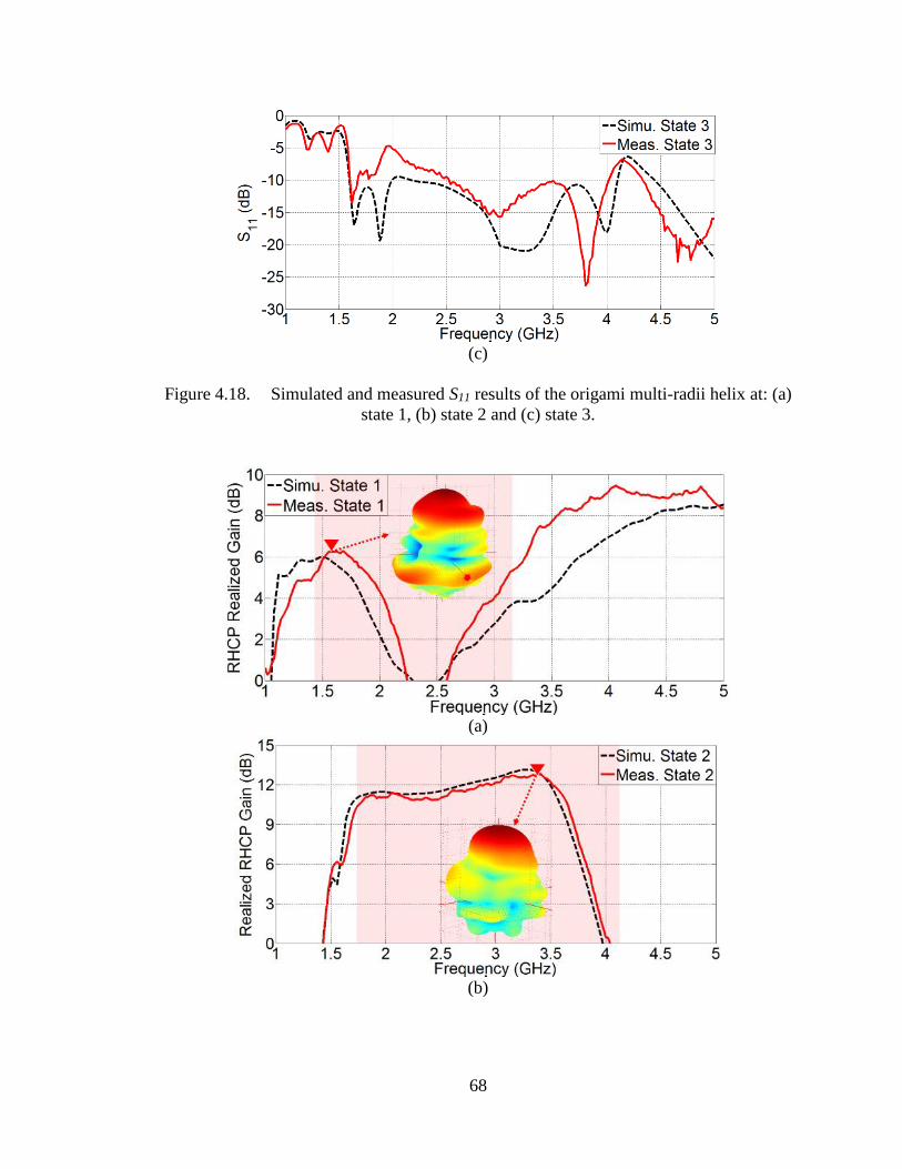
68

(c)

Figure 4.18. Simulated and measured S11 results of the origami multi-radii helix at: (a)

state 1, (b) state 2 and (c) state 3.

(a)

(b)

69

(c)

Figure 4.19. Simulated and measured realized RHCP gain of the origami multi-radii

helix at: (a) state 1, (b) state 2 and (c) state 3.

(a)

(b)

70

(c)

Figure 4.20. Simulated and measured axial ratio of the origami multi-radii helix at: (a)

state 1, (b) state 2 and (c) state 3.

(a)

71

(b)

(c)

Figure 4.21. Simulated and measured elevational radiation patterns of the origami

multi-radii helix at: (a) state 1 at 1.56 GHz, (b) state 2 at 3.16 GHz, and (c) state 3 at

3.88 GHz.

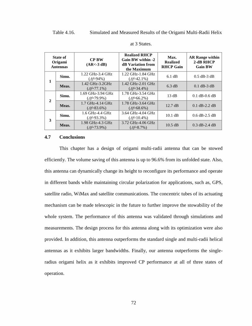
72

Table 4.16. Simulated and Measured Results of the Origami Multi-Radii Helix

at 3 States.

State of

Origami

Antennas

CP BW

(AR<-3 dB)

Realized RHCP

Gain BW within -2

dB Variation from

the Maximum

Max.

Realized

RHCP Gain

AR Range within

2-dB RHCP

Gain BW

1

Simu. 1.22 GHz-3.4 GHz

(Δf=94%)

1.22 GHz-1.84 GHz

(Δf=42.1%) 6.1 dB 0.5 dB-3 dB

Meas. 1.42 GHz-3.2GHz

(Δf=77.1%)

1.42 GHz-2.01 GHz

(Δf=34.4%) 6.3 dB 0.1 dB-3 dB

2


(Δf=79.9%)

1.78 GHz-3.54 GHz

(Δf=66.2%) 13 dB 0.1 dB-0.6 dB

Meas. 1.7 GHz-4.14 GHz

(Δf=83.6%)

1.78 GHz-3.64 GHz

(Δf=68.6%) 12.7 dB 0.1 dB-2.2 dB

3


(Δf=93.3%)

3.64 GHz-4.04 GHz

(Δf=10.4%) 10.1 dB 0.6 dB-2.5 dB

Meas. 1.98 GHz-4.3 GHz

(Δf=73.9%)

3.72 GHz-4.06 GHz

(Δf=8.7%) 10.5 dB 0.3 dB-2.4 dB

4.7 Conclusions

This chapter has a design of origami multi-radii antenna that can be stowed

efficiently. The volume saving of this antenna is up to 96.6% from its unfolded state. Also,

this antenna can dynamically change its height to reconfigure its performance and operate

in different bands while maintaining circular polarization for applications, such as, GPS,

satellite radio, WiMax and satellite communications. The concentric tubes of its actuating

mechanism can be made telescopic in the future to further improve the stowability of the

whole system. The performance of this antenna was validated through simulations and

measurements. The design process for this antenna along with its optimization were also

provided. In addition, this antenna outperforms the standard single and multi-radii helical

antennas as it exhibits larger bandwidths. Finally, our antenna outperforms the single-

radius origami helix as it exhibits improved CP performance at all of three states of

operation.

73

CHAPTER 5

REFLECTOR RECONFIGURABLE ORIGAMI QUADRIFILAR AND MONOFILAR

HELICAL ANTENNA FOR SATELLITE COMMUNICATIONS

5.1 Origami QHA with Reflector

This section presents a design of a circularly polarized origami Quadrifilar Helical

Antenna (QHA) with a reconfigurable reflector that can operate at 3 states in K, Ka, and

EHF bands. The K, Ka, and EHF bands employ millimeter wavelengths and can support

high bandwidth transmissions using small receiving antennas [41]. The proposed reflector

and QHA are able to reconfigure themselves at three different states using origami folding.

A 10:1 scale model of the proposed origami QHA is manufactured and measured in order

to validate our design.

5.1.1 Design of Origami QHA

The QHA is designed to operate in axial mode. Empirically, the optimum

circumference and pitch size for a circularly polarized helical antenna in axial mode should

be 0.75λ0<C<1.33λ0, and S=0.25λ0, where λ0 is the wavelength at its operating frequency,

C is the circumference of the helix and S is the spacing between each turn [13]. Therefore,

a helical antenna with fixed total length can achieve a frequency reconfigurability by

changing its pitch, S. Here, an origami QHA is proposed in order to achieve frequency

reconfigurability for K, Ka and EHF bands.

The origami pattern used to fold the cylinder base of the QHA is shown in Figure

5.1. The number of sides, n, is picked to be equal to 4 in order to enable symmetric

placement of the four helical arms of the QHA around the origami cylinder.

74

Figure 5.1. Origami folding pattern of the QHA cylinder base.

The 3-D QHA model is shown in Figure 5.2. The QHA is fed using a progressive

90° phase difference from port to port counter-clockwisely (as shown in Figure 5.2) in

order to achieve a right-hand circular polarization. The total height, H, of the QHA can be

adjusted to change its operating frequency from 20.7 GHz to 30 GHz and 44.5 GHz in K,

Ka and EHF bands, respectively. It should be noted that when H is decreased, the number

of turns N is increased, as expressed below:

na

HbmN

222 (1)

Figure 5.2. Origami quadrifilar helical antenna model.

75

5.1.2 Design of the Origami Reflector

The impact of various reflectors on the performance of helical antennas has been

previously studied [47]. The truncated-cone ground provides the highest gain for helical

antennas compared to square, cylindrical-cup, and conical grounds [47].

Based on the truncated-cone ground, a novel foldable truncated-heptahedron

reflector is proposed in this paper, which can reconfigure to cover the three operating bands

of the proposed QHA. The geometries of the three reconfigurable states of the reflector

QHA are shown in Figure 5.3 along with the corresponding folding patterns of the reflector,

where red dashed lines represent valleys, blue dash-dot lines are hills and green solid lines

are outlines.

(a) State 1 at 20.7 GHz.

(b) State 2 at 30 GHz.

76

(c) State 3 at 44.5 GHz.

Figure 5.3. The three states of the reconfigurable origami QHA with the foldable

reflector and the folding patterns of the reflector.

5.1.3 Simulation Results

This reflector QHA antenna was modeled and analyzed in ANSYS HFSS. The

simulated S11, realized RHCP gain, and axial ratio are shown in Figure 5.4-Figure 5.6.

Figure 5.4 shows that the designed reconfigurable origami QHA with the reflector has a

return loss greater than 15 dB in all three states. Also, the three states of the designed

antenna are circularly polarized and they have a realized RHCP gain higher than 15 dB at

their operating frequencies, as shown in Figure 5.4-Figure 5.6.

Figure 5.4. Simulated S11 of the reconfigurable origami QHA with the reflector at

three states.

77

Figure 5.5. Simulated realized RHCP gain of the reconfigurable origami QHA with

the reflector at three states.

Figure 5.7 shows that the reflector QHA exhibits the best performance in terms of

gain and pattern at the operating frequency of each state compared to the other two states.

It should be pointed out that Figure 5.5 shows that the first state (corresponding to K-band

operation, H=13.6 mm) exhibits approximately the same gain as the second state

(corresponding to Ka-band operation, H=11.9 mm) at the Ka band and a higher gain than

the gain of the third state (corresponding to EHF-band operation, H=5 mm) at the EHF

band. However, the radiation patterns of the first state (see Figure 5.7), exhibit large side

lobes at Ka band (8.9 dB) and EHF band (5.2 dB) and therefore, the first state cannot be

used in the Ka and EHF bands.

Figure 5.6. Simulated axial ratio of the reconfigurable origami QHA with the reflector

at three states.

78

(a) 20.7 GHz. (b) 30 GHz.

(c) 44.5 GHz.

Figure 5.7. RHCP patterns at three states of the reconfigurable origami reflector QHA

at designated operating frequencies.

To prove that 3 configurations of the reflector are necessary to optimize the QHA

performances at the 3 operating frequencies, simulated RHCP patterns of the QHA at

3 reconfigurable states of height resonating at the designated operating frequencies with

one common reflector state are shown in Figure 5.8 for 3 common reflector states. It can

be seen from Figure 5.8 that although the QHA performance can be optimized at one of

operating frequencies with the common reflector, the radiation patterns at the other 2

reconfigurable frequencies can’t be as good due to larger side lobes or lower gains.

Therefore, 3 states of the reflector were optimized for each operating frequency, as

introduced earlier in § 5.1.2.

79

(a) Reflector at state 1 (b) Reflector at state 2 (c) Reflector at state 3

Figure 5.8. RHCP patterns of reconfigurable QHA resonating at 3 designated

operating frequencies with one common reflector state.

5.1.4 10:1 Scale Model of Origami QHA

The size of the proposed origami QHA is too small; therefore, it is difficult to build

its prototype by hand, and new manufacturing techniques need to be explored. Therefore,

we decided to build a 10:1 scale model of the proposed origami QHA in order to validate

its performance. The 10:1 scale QHA will operate at the operating frequencies of 2.07 GHz,

3 GHz and 4.45 GHz. Since the SMA connector feed slightly decreases the resonant

frequencies of the antenna, the initial 10:1 scale dimensions of the origami pattern and

QHA model are slightly adjusted (a increased by 1.2 mm, b increased by 0.8 mm, m

decreased by 2) in order to compensate this effect of the SMA connector feed and tune the

QHA at the scaled frequencies, as shown in Figure 5.9. Also, the dimensions of the 10:1

scale reflector were slightly adjusted through simulations to provide optimal performance

for each state of the slightly adjusted 10:1 scale QHA, as shown in Figure 5.10.

80

(a) (b)

Figure 5.9. Geometry of the 10:1 scale model of the origami QHA. (a) origami

folding pattern, and (b) 3D model.

(a) (b) (c)

Figure 5.10. Geometry of 10:1 scale model of the origami QHA with its reflector at

three states: (a) state 1 (H=120 mm); (b) state 2 (H=75 mm); (c) state 3 (H=105 mm).

The prototype of the 10:1 scale reflector of the QHA was manufactured and its three

states are shown in Figure 5.11. The 10:1 scale QHA was constructed by attaching copper

tape (arms of the QHA) on sketching paper and folding the paper base into an origami

cylinder, as shown in Figure 5.9(a). The 10:1 scale reflector was constructed by gluing

copper foil on a single piece of sketching paper. This reflector can be reconfigured into

81

three different states following the folding pattern shown in Figure 5.3. The QHA prototype

can be reconfigured by applying a force at the top of the origami helix to adjust its height

from state 1 to state 3. Also the reflector prototype was reconfigured manually in

measurements.

(a) State 1 (H=120 mm) (b) State 2 (H=75 mm) (c) State 3 (H=105 mm)

Figure 5.11. Geometry of 10:1 scale model of the origami QHA with its reflector.

The S-parameters were measured using an E5071C Agilent network analyzer.

Figure 5.12 compares the simulated and measured S11 for the 3 states. The feeding network

is constructed using one 180° hybrid coupler and two 90° hybrid couplers. The radiation

pattern and gain measurements were performed using a Diamond Engineering antenna

measurement system.

(a) State 1 (operating frequency, f0=2.07 GHz)

82

(b) State 2 (operating frequency, f0=3 GHz)

(c) State 3 (operating frequency, f0=4.45 GHz)

Figure 5.12. Comparison of simulated and measured S11 at the three states.

The simulated and measured radiation patterns of the 3 states are compared in

Figure 5.13. Also, the simulated and measured realized RHCP gains and axial ratios are

listed in Table 5.1 at 2.07 GHz, 3 GHz and 4.45 GHz. Figure 5.13 shows that the reflector

origami QHA operates in axial mode at the 3 states, and Table 5.1 shows that this antenna

is right-hand circularly polarized with measured gains over 12 dB. Compared to the

proposed design in section II, this 10:1 scale model has successfully enlarged its operating

wavelength by 10 times to operate at 2.07 GHz, 3 GHz and 4.45 GHz, as shown in Table

5.1.

83

(a) (b) (c)

Figure 5.13. Simulated and measured normalized radiation patterns at the three states:

(a) state 1 at 2.07 GHz, (b) state 2 at 3 GHz, and (c) state 3 at 4.45 GHz.

Table 5.1 Simulated and Measured Results at Designated Frequencies of the 10:1

Scale Antenna.

Reconfigurable State State 1

(H=120 mm)

State 2

(H=75 mm)

State 3

(H=105 mm)

Center Operating Frequency (GHz) 2.07 3.00 4.45

Simulated Realized RHCP Gain (dB) 13.87 12.50 15.41

Measured Realized RHCP Gain (dB) 13.20 12.13 14.86

Simulated AR (dB) 0.04 0.11 0.03

Measured AR (dB) 0.66 0.09 0.55

5.1.5 Conclusion

Section 5.1 presents a design of an origami RHCP QHA with a foldable reflector

that can reconfigure itself to operate in three different bands, namely K, Ka and EHF.

Simulated and measured results of a 10:1 scale model of this antenna validated the

reconfigurable performance of this antenna at the three bands. Our future work will focus

on robust manufacturing of this reconfigurable origami QHA for the K, Ka and EHF bands.

84

5.2 Tri-band Reconfigurable Origami Helical Array

5.2.1 Geometry of Single Helical Antenna Element

According to antenna theory, to achieve the optimum CP performance in a helical

antenna, the length of one turn of the helix should be approximately equal to one

wavelength [37]. However, this condition could not be satisfied at all the reconfiguration

states of an origami monofilar. Therefore, a smaller helical section is added for each

element to achieve CP. The folding pattern of single element is shown in Figure 5.14 (a),

and the folded origami monofilar is shown in Figure 5.14 (b). The values of the geometrical

parameters of this helical antenna are listed in Table 5.2. Thus, the diameters of the

monofilar are: d1=27.2 mm and d=34 mm. The height of one turn in the two helical sections

(pitch and pitch1), and the number of turns of the two helical sections (N and N1) can be

varied by changing their folding angles [29] in order to achieve frequency reconfiguration

and CP at the three states (see § 5.2.3).

Table 5.2 Geometrical Parameters of Single Helical Element.

m m1 n a w fscale ratio

15 6 4 24 mm 16 mm 0.8 0.85

5.2.2 Geometry of Single Reflector Element

The single reflector element is shown in Figure 5.14, and its geometrical parameters

are listed in Table 5.3. The geometry of the reflector can be solely determined by its angle

to the ground α and the side length of bottom hexagon amin. We chose a common reflector

for all three operational states with amin=50 mm and α=40° for compromised maximum

gains at the 3 states.

85

(a) (b)

Figure 5.14. Geometry of single reflector element: (a) top view; and (b) side view.

Table 5.3 Geometrical parameters of Single Reflector Element.

α amin amax dmin dmax l v Hreflector

40° 50 mm 101 mm 86.6 mm 175 mm 57.7 mm 63.1 mm 37 mm

5.2.3 Geometry of 7-element Array

The 3 states of the 7-element multi-radii origami helical array are shown in Figure

5.15 with the distance between elements being set to gap=5 mm. The geometrical

parameters and number of turns at each state are listed in Table 5.4.

(a) (b) (c)

Figure 5.15. Antenna array model at: (a) state 1, (b) state 2 and (c) state 3.

Table 5.4 Geometrical parameters at Each State.

State 1 (fc=2.07 GHz) State 2 (fc=3 GHz) State 3 (fc=4.45 GHz)

pitch 80 mm 50 mm 15 mm

pitch1 65 mm 25 mm 10 mm

N 2.45 2.83 3.15

N1 1.14 1.41 1.48

86

5.2.4 Fabrication of Prototype

The helical antenna elements are fabricated with 3-mil thick copper tape glued on

6.5-mil thick sketching paper, and the reflector elements are fabricated with 4-mil thick

copper foil glued on 13-mil thick cardboard, as shown in Figure 5.16.

Figure 5.16. Fabricated prototype of the 7-element origami helical array.

5.2.5 Simulated and Measured Results

The performance of the proposed helical array is verified by the simulated and

measured results as shown in Table 5.5 and Figure 5.17.

(a) (b) (c)

Figure 5.17. Simulated and measured radiation patterns of the helical array at (a) state 1

at 2.07 GHz, (b) state 2 at 3 GHz and (c) state 3 at 4.45 GHz.

87

Table 5.5 Simulated and Measured Results of the Array.

State 1

(fc=2.07 GHz)

State 2

(fc=3 GHz)

State 3

(fc=4.45 GHz)

Meas. Simu. Meas. Simu. Meas. Simu.

S11 (dB) < -14 < -2.1 < -10 < -9.3 < -12 < -45

Polarization RHCP RHCP RHCP RHCP RHCP RHCP

Gaintotal (dB) 9.7 11.6 13 13.3 14.7 15.7

Zenithal AR (dB) 1.35 0.76 1.17 0.85 0.64 0.69

88

CHAPTER 6

OTHER ORIGAMI ANTENNA STRUCTURES

6.1 Mode Reconfigurable Bistable Spiral Antenna Based on Kresling Origami

Conical spiral antennas with two or four arms are often used due to their symmetry

and zenithal directional radiation patterns [48]. Based on Kresling origami, a conical spiral

antenna is developed that does not need mechanical support after is deployed because of

the buckling of a thin cylindrical or conical shell under torsional loading [32]. Also, this

antenna can be very compact without any hinges and can be easily fabricated from a planar

origami pattern to a 3-D conical spiral antenna, providing a low-cost and potentially

disposable design. Also, here we demonstrate a general analytical method for designing

bistable conical or cylindrical Kresling origami and show the performance a mode-

reconfigurable spiral antenna based on a Kresling origami pattern.

6.1.1 Kresling Conical or Cylindrical Origami

The geometry of a 6-side Kresling origami and the top view and perspective view

of one if its steps is shown in Figure 6.1. We define b ratio a , and the scaling factor

between adjacent steps so that scalea f a . We have concluded in [29] that

n

a

bh180

sin

2sin

2

22

2

(1)

Similarly, for an ordinary origami pattern with scaling factor scalef for each step, we have:

89

2

2

2

sin2

sinscaleh a f ratio

(2)

where α=π/n is the internal angle of the polygon at the cross section of the origami step in

Figure 6.1. In a rectangular coordinate system, the lower point A with diagonal length c of

the first step in Figure 6.1 has coordinates ( ,0,0)2sin( / 2)

a

. Then, the upper point B can be

has coordinates cos( ) sin( )

( , , )2sin( / 2) 2sin( / 2)

scale scalea f a fh

.

Therefore, we can calculate the length of c and express it with its ratio to the length

of a. Based on the method stated above and using the strain energy [32], we are able to find

an origami pattern with a suitable fscale=0.83, and ratio=1.6 that provides a bistable

structure and buckles when =34 and =106.25.

(a) (b)

Figure 6.1 (a) Kresling origami pattern, (b) Top view and perspective view of one

step of the pattern.

90

(a) Conical spiral (b) Planar spiral

Figure 6.2 Model of the conical and planar spiral antenna.

6.1.2 Simulated Results

The simulated model is shown in Figure 6.2. The two SMA ports are fed out of

phase (0° and 180°), and the ground plane is omitted so as not to interfere with the

bidirectional radiation pattern of the planar spiral antenna when it is collapsed. Ideally, the

height of this planar state can be as small as 1.8 mm in simulation.

The simulated realized gain is shown in Figure 6.3. At the unfolded state, the

conical spiral antenna is circularly polarized from 2.5 GHz to 3.2 GHz. The radiation

patterns of the two states at 2.7 GHz are shown in Figure 6.4.

Figure 6.3 Simulated realized gain at the two states.

150H mm

91

(a) (b)

Figure 6.4 Radiation patterns at 2.7 GHz: (a) conical spiral; (b) planar spiral.

Figure 6.5 Front to back ratio at the two states.

6.2 A Frequency Tunable Origami Spherical Helical Antenna

Spherically folded helical antennas are suitable for developing electrically small

antennas, and they have radiation patterns similar with an electric dipole or a magnetic

dipole [49]. However, such antennas have high Q-factors. Therefore, their maximum

bandwidths are limited since 0ff

Q . Research has been carried out on how to decrease

the Q-factor of electrically small antennas and increase their bandwidth [49]. A novel

spherical antenna structure and novel prototyping method have been proposed in [50]. It

has been found that by adjusting the number of arms M, number of turns N and the

dimension of the sphere, the impedance of a spherical antenna can be tuned with less

reactance [51]. Specifically, increasing M alone increases the antenna’s capacitance,

increasing N alone increases its inductance, while the more closely the antenna is winded

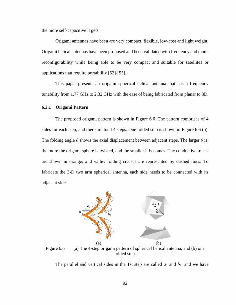
92

the more self-capacitive it gets.

Origami antennas have been are very compact, flexible, low-cost and light weight.

Origami helical antennas have been proposed and been validated with frequency and mode

reconfigurability while being able to be very compact and suitable for satellites or

applications that require portability [52]-[55].

This paper presents an origami spherical helical antenna that has a frequency

tunability from 1.77 GHz to 2.32 GHz with the ease of being fabricated from planar to 3D.

6.2.1 Origami Pattern

The proposed origami pattern is shown in Figure 6.6. The pattern comprises of 4

sides for each step, and there are total 4 steps. One folded step is shown in Figure 6.6 (b).

The folding angle θ shows the axial displacement between adjacent steps. The larger θ is,

the more the origami sphere is twisted, and the smaller it becomes. The conductive traces

are shown in orange, and valley folding creases are represented by dashed lines. To

fabricate the 3-D two arm spherical antenna, each side needs to be connected with its

adjacent sides.

(a) (b)

Figure 6.6 (a) The 4-step origami pattern of spherical helical antenna; and (b) one

folded step.

The parallel and vertical sides in the 1st step are called a1 and b1, and we have

93

1 1b ratio a . For the 2nd step, 2 1 1scalea f a , and so on. A different scaling factor is chosen

for each step to mimic an origami sphere. The parameters are: a1=21.2 mm, 0.7ratio ,

1 0.9scalef , 2 0.75scalef , 3 0.6scalef , 4 0.5scalef .

6.2.2 Simulated Model and Results

The four states of folded 3-D spherical antenna are shown in Figure 6.7. A two-arm

spherical helix works better than one-arm and four-arm helices, because it has less

reactance. Also, the reactance of a two-arm spherical helix has a larger range of tunability

as h changes. When the antenna collapses from state 1 to state 4, the number of turns of

each arm changes from about 1 to 1.5 while the total wire length stays the same. The

antenna is fed at the center of one arm with all other parts connected together.

(a) (b) (c) (d)

Figure 6.7 The 4 states of the spherical antenna: (a) state1 (h=8.69 mm); (b) state 2

(h=21.8 mm); (c) state 3 (h=11.6 mm); and (d) state 4 (h=6.5 mm).

Figure 6.8 The simulated S11 at the 4 states of height.

94

The S11 of the 4 states are shown in Figure 6.8, and the radiation patterns of the four

states at their operating frequencies are shown in Figure 6.9. The maximum realized gain

at operating frequencies of the 4 states of height are: 2.9 dB at 2.32 GHz at state 1, 1.4 dB

at 1.77 GHz at state 2, 2.9 dB at 2.07 GHz at state 3 and 3 dB at 2.12 GHz at state 4. The

radiation pattern at state 1 is in the vertical plane, because the mutual coupling between the

turns is small and therefore, the antenna operates like a loop antenna.

(a) (b) (c) (d)

Figure 6.9 Simulated radiation patterns of the 4 states at their resonant frequencies:

(a) h=28.6 mm at 2.32 GHz; (b) h=21.8 mm at 1.77 GHz; (c) h=11.6 mm at 2.07 GHz;

(d) h=6.5 mm at 2.12 GHz.

6.2.3 Conclusion

A frequency reconfigurable normal mode spherical antenna is proposed and it has

a potential to be applied in radio or TV communications. Also, the fabricating process is

simple as to put conductive layer along the creases and then fold it up. Therefore, a low-

cost and lightweight design is provided.

95

CHAPTER 7

CONCLUSION AND FUTURE WORK

7.1 Conclusions

This dissertation presented research of origami antennas for novel reconfigurable

communication systems. Reconfigurable monofilar, bifilar and quadrifilar antennas based

on origami cylinders were proposed and validated. Novel fabrications of practical designs

were presented with detailed geometrical analysis. In addition, multi-radii origami

antennas were proposed, analyzed, fabricated and validated and they exhibit very good

circular polarization performance and wide bandwidths at the 3 reconfigurable states. Also,

an actuation mechanism was developed for this antenna.

A low-cost and lightweight reconfigurable origami antenna with a reflector and an

array of this antenna were proposed to improve antenna gain at multiple states. Also, a

Kresling conical spiral antenna and a spherical helical antenna were designed with mode

reconfigurabilities and validated by simulated results.

These origami structures can easily reconfigure their heights to operate in various

resonant frequencies or different radiation modes, and they can achieve large volume

savings when they are stowed. Also, our origami antennas can be applied in novel

communication and sensing applications requiring lightweight and multi-functional

systems and real-time reconfigurability.

7.2 Future Work

Novel fabrication processes and new materials need to be studied for developing

robust origami antennas that can maintain their mechanical functionality through a large

96

number of deployment/stowage cycles. Also, inflatable reconfigurable origami antennas

can be developed to make new actuation systems.

In addition, other types of antennas, such as, Vivaldi antennas and patch arrays, can

be embodied on reconfigurable origami structures for stowability and multi-functionality.

97

REFERENCES

[1] Y. Akira, “Atarashii Origami Geijutsu,” Tokyo: Origami Geijutsusha, 1954.

[2] P. Engel, “Origami from Angelfish to Zen,” Dover Publications, 1994.

[3] S. D. Guest and S. Pellegrino, “The Folding of Triangulated Cylinder, Part I,

Geometric Considerations,” J. of Appl., vol. 61, pp. 773-777, 1994.

[4] B. A. Cipra, “In the Fold; Origami Meets Mathematics,” SIAM News, vol. 34, 2002.

[5] T. Nojima, “Origami Modeling of Functional Structures based on Organic Patterns”,

Kyoto University.

[6] Erik D. DemaineJoseph O'Rourke, “Geometric Folding Algorithms: Linkages,

Origami, Polyhedra,” Cambridge University Press New York, NY, USA, 2007.

[7] J. P. Gardner, et, “The James Webb Space Telescope,” Space Sci. Reviews, vol.

123, pp. 485-606, May 2006.

[8] K. Kuribayashi, K. Tsuchiya, Z. You, D. Tomus, M. Umemoto, T. Ito and M.

Sasaki, “Self-deployable Origami Stent Grafts as a Biomedical Application of Ni-

rich TiNi Shape Memory Alloy Foil”, Mater. Sci. Eng., vol. 419, pp. 131-137, 2006.

[9] R. Hoffmann, A. K. Pickett, D. Ulrich, E. Haug, D. Lasry and J. Clinkemailllie, “A

Finite Element Approach to Occupant Simulation: the PAM-CRASH Airbag

Model”, Automotive frontal impacts, pp. 79-87, 1989.

[10] Mark Schenk, Andrew D. Viquerat, Keith A. Seffen and Simon D. Guest, “Review

of Infatable Booms for Deployable Space Structures: Packing and Rigidization,”

Journal of Spacecraft and Rockets, vol. 51, no. 3, pp. 762-778, 2014.

[11] K. Kuribayashi, H. Onoe and S. Takeuchi, “Cell Origami: Self-Folding of Three-

Dimensional Cell-Laden Microstructures Driven by Cell Traction Force,” PLOS

One, vol. 7, no. 12, Dec. 2006.

[12] S. Felton, M. Tolley, E. Demaine, D. Rus and R. Wood, “A Method for Building

Self-Folding Machines,” Sci., vol. 345, pp. 644-646, 2014.

[13] C. A. Balanis, “Antenna Theory Analysis and Design,” 3rd ed. Hoboken, NJ, USA:

Wiley, 2005.

[14] R. H. Patnam, “Broadband CPW-Fed Planar Koch Fractal Loop Antenna,” IEEE

Antennas Wireless Propag. Lett., vol. 7, pp. 429-431, 2008

https://dl.acm.org/author_page.cfm?id=81100553346&coll=DL&dl=ACM&trk=0

https://dl.acm.org/author_page.cfm?id=81100553346&coll=DL&dl=ACM&trk=0

98

[15] G. J. Hayes, Y. Liu, J. Genzer, G. Lazzi and M. D. Dickey, “Self-Folding Origami

Microstrip Antennas,” IEEE Antennas Wireless Propag. Lett., vol. 62, no. 10, pp.

5416–5419, 2014.

[16] Selding, P. “Boeing Finishes Deployment of Stuck SkyTerra 1 Antenna,” Space

News, Dec. 2012.

[17] R. C. Gupta, S. K. Sagi, K. P. Raja, N. K. Sharma and R. Jyoti, “Shaped Prime-

Focus Reflector Antenna for Satellite Communication,” IEEE Antennas Wireless

Propag. Lett., vol. 16, pp. 1945-1946, 2017.

[18] T. K. Sreeja, A. Arun and J. Jaya Kumari, “An S-band Micro-Strip Patch Array

Antenna for Nano-Satellite Applications,” ICGT Internat. Conf., pp. 325-328,

Trivandrum, India, Dec. 2012.

[19] S. K. Podilchak, A. P. Murdoch and Y. M.M. Antar, “Compact, Microstrip-Based

Folded-Shorted Patches: PCB Antennas for Use on Microsatellites,” IEEE

Antennas and Propag. Magazine, vol. 59, no. 2, pp. 88-95, 2017.

[20] G. M. Olson, S. Pellegrino, J. Costantine and J. Banik, “Structure Architectures for

a Deployable Wideband UHF Antenna,” 53rd AIAA/ASME/ASCE/AHS structure,

structural dynamics mater. conf., Hawaii, 2012.

[21] N. Robinson, “The Origami Bible,” North Light Books, 2004.

[22] R. J. Lang, “The Complete Book of Origami: Step-by Step Instructions in Over 1000

Diagrams/37 Original Models,” Courier Dover Publications, 1988.

[23] Z. Abel, J. Cantarella, E. D. Demaine, D. Eppstein, Thomas C. Hull, Jason S. Ku,

Robert J. Lang and Tomohiro Tachi, “Rigid Origami Vertices: Conditions and

Forcing Sets,” J. of Computational Geometry, vol. 7, no. 1 (2016): 171-184.

[24] Cheng Lv, “Theoretical and Finite Element Analysis of Origami and Kirigami

Based Structures,” Dissertation for the Doctor of Philosophy Degree, Arizona State

University, August 2016.

[25] C. M. Kruesi, R. J. Vyas and M. M. Tentzeris, “Design and development of a novel

3-D cubic antenna for wireless sensor networks and RFID applications,” IEEE

Trans. Antennas Propag., vol. 57, no. 10, pp. 3293-3299, 2009.

[26] H. Hu and S. V. Georgakopoulos, “Wireless Powering Based on Strongly Coupled

Magnetic Resonance with SRR Elements,” IEEE Antennas Propagat. Soc. Internat.

Symp., Chicago, IL, Jul. 2012.

[27] C. A. Balanis, “Travelling wave and broad band antennas,” Antenna Theory

Analysis and Design, 3rd ed., chap 10, (New Jersey: Hoboken, 2005): 566-572.

99

[28] A. R. Djordjević, A. G. Zajić, M. M. Ilić, and G. L. Stüber, “Optimization of

Helical Antennas,” IEEE Antennas and Propagation Magazine, vol. 48, no. 6

(2006): 107-116.

[29] X. Liu, S. Yao, B. S. Cook, M. M. Tentzeris, and S. V. Georgakopoulos, “An

origami reconfigurable axial-mode bifilar helical antenna,” IEEE Trans. on Ant.

and Propag., vol. 63, no. 12, pp. 5897-5903, Dec. 2015.

[30] J. Zhong, A. Kiourti, T. Sebastian,Y. Bayram and J. L. Volakis, “Conformal load-

bearing spiral antenna on conductive textile threads,” IEEE Ant. & Wireless Propag.

Lett., vol. 16, pp. 230-233, May, 2016.

[31] S. D. Guest and S. Pellegrino, “The Folding of Triangulated Cylinders, Part III:

Experiments”, Journal of Applied Mechanics. Vol. 63 (1), pp. 77-83, 1996.

[32] C. Jiangguo, D. Xiaowei, Z. Ya, F. Jian and T. Yongming, “Bistable Behavior of

the Cylindrical Origami Structure with Kresling Pattern”, Journal of Mechanical

Design, vol. 137, no. 061406, pp. 1-8, June 2015.

[33] S. Yao, X. Liu and S. V. Georgakopoulos, “Morphing origami conical spiral

antenna based on the Nojima wrap,” IEEE Trans. on Ant. and Propag., vol. 65, no.

5, pp. 2222-2232, May. 2017.

[34] J. Costantine, Y. Tawk, I. Maqueda, M. Sakovsky, G. Olson, S. Pellegrino and C.

G. Christodoulou, “UHF Deployable Helical Antennas for CubeSats,” IEEE Trans.

on Ant. and Propag., vol. 64, no. 9, pp. 3752-3759, Sept. 2016.

[35] S. I. H. Shah, M. M. Tentzeris and S. Lim, “Low-cost Circularly Polarized Origami

Antenna,” IEEE Ant. and Wireless Propag. Lett., vol. 16, pp. 2026-2029, Apr. 2017.

[36] J. L. Wong and H. E. King, “Broadband Quasi-taper Helical Antennas,” IEEE

Trans. on Ant. and Propag., vol. AP-27, no. 1, pp. 72-78, Jan. 1979.

[37] Antenna theory and design, 3rd ed., John Wiley & Sons, Inc., Hoboken, MA, 2012,

pp. 217-219.

[38] F. Falzon and P. Blanc, “Deployable reflector in the form of a reuleaux triangle for

a space observation instrument,” U.S. Patent 007839567B2, Nov. 23, 2010.

[39] D. Heitmann, “Round reflector for electromagnetic radiation,” U.S. Patent

008277086B2, Oct. 2, 2012.

[40] L. Stiles, J. Garrett, Th. Murphey, H. Dumm, and J. Banik, “Development of

deployable aperture concepts for CubeSats,” in 51st

AIAA/ASME/ASCE/AHS/ASC Structures, Structural Dynamics, and Materials

Conf., Orlando, 2010, pp. 1-10.

100

[41] Bruce R. Elbert, “Frequency spectrum allocations,” in Introduction to Satellite

Communication, 3rd ed., ch. 1, Artech House, Inc. Massachusetts: Norwood, 2008,

pp. 22-38.

[42] X. Liu, S. Yao, and S. V. Georgakopoulos, “Reconfigurable spherical helical

Electrically Small Antenna in UHF band,” in Antennas and Propagation Society Int.

Symposium (APSURSI), Memphis, 2014, pp. 368-369.

[43] S. Yao, X. Liu, S. V. Georgakopoulos, and M. M. Tentzeris, “A novel tunable

origami accordion antenna,” in Antennas and Propagation Society Int. Symposium

(APSURSI), Memphis, 2014, pp. 370-371.

[44] X. Liu, S. Yao, S. V. Georgakopoulos, and M. M. Tentzeris, “Origami Quadrifilar

Helix Antenna in UHF band,” in Antennas and Propagation Society Int.


[45] S. Yao, X. Liu, S. V. Georgakopoulos, and M. M. Tentzeris, “A novel

reconfigurable origami spring antenna,” in Antennas and Propagation Society Int.


[46] X. Liu, S. Yao, S.V. Georgakopoulos, B. S. Cook, and M. M. Tentzeris,

“Reconfigurable helical antenna based on an origami structure for wireless

communication system,” in 2014 IEEE MTT-S Int. Microwave Symposium (IMS),

Tampa, 2014, pp. 1-4.

[47] A. R. Djordjevic, A. G. Zajic and M. M. Ilic, “Enhancing the gain of helical

antennas by shaping the ground conductor,” IEEE Antennas and Wireless Propagat.

Letters, vol. 5, pp. 138-140, Dec. 2006.

[48] A. J. Ernest, Y. Tawk, J. Costantine, and C. G. Christodoulou, “A bottom fed

deployable conical log spiral antenna design for cubeSat”, IEEE Antennas

Propagat., vol. 63, no. 1, pp. 41-47, January 2015.

[49] O. S. Kim, “Minimum electrically small antennas”, IEEE Trans. on Ant. and

Propag., vol. 60, no. 8, pp. 3551-3558, August 2012.

[50] O. S. Kim, “Rapid prototyping of electrically small spherical wire antennas”, IEEE

Trans. on Ant. and Propag., vol. 62, no. 7, pp. 3839-3842, July 2014.

[51] H. Huang, K. Nieman, Y. Hu and D. Akinwande, “Electrically small folded

elliptical antenna for medical implanted applicaton,” 2011 IEEE International

Symposium on Antennas and Propagation (APSURSI), pp. 769–771, 2011.

[52] X. Liu, S. Yao, S. V. Georgakopoulos, "Frequency reconfigurable origami

quadrifilar helical antenna with reconfigurable reflector.” ", IEEE Antennas

Propagat. Society Internat. Symp., pp 2217-2218, Jul. 19-24, 2015.

http://ieeexplore.ieee.org/search/searchresult.jsp?searchWithin=p_Authors:.QT.Xueli%20Liu.QT.&newsearch=true

http://ieeexplore.ieee.org/search/searchresult.jsp?searchWithin=p_Authors:.QT.Shun%20Yao.QT.&newsearch=true




http://ieeexplore.ieee.org/search/searchresult.jsp?searchWithin=p_Authors:.QT.Shun%20Yao.QT.&newsearch=true

http://ieeexplore.ieee.org/search/searchresult.jsp?searchWithin=p_Authors:.QT.Georgakopoulos,%20S.V..QT.&newsearch=true

http://ieeexplore.ieee.org/xpl/mostRecentIssue.jsp?punumber=6842514

101

[53] S. Yao, X. Liu and S. V. Georgakopoulos, “Study and design of Nojima origami

conical spiral antenna,” IEEE Antennas Propagat. Society Internat. Symp., pp

1431-1432, 2016.

[54] X. Liu, S. Yao and S. V. Georgakopoulos, "Reconfigurable origami equiangular

conical spiral antenna", IEEE Antennas Propagat. Society Internat. Symp., pp

2263-2264, Jul. 19-24, 2015.

[55] X. Liu, S. Yao, P. Gonzalez and S. V. Georgakopoulos, “A novel ultra-wideband

origami reconfigurable quasi-taper helical antenna”, IEEE Antennas Propagat.

Society Internat. Symp., pp 839-840, Jul. 19-24, 2015.

102

VITA

XUELI LIU

2005-2009 B. S., Applied Physics

University of Electronic Science and Technology of China

Chengdu, China

2009-2012 M. S., Electromagnetic Field and Microwave Technology

University of Electronic Science and Technology of China

Chengdu, China

2013-2018 Ph. D. Candidate, Electrical Engineering

Florida International University

Miami, Florida

PUBLICATIONS and PRESENTATIONS

[1] S. V. Georgakopoulos, X. Liu and S. Yao, “Origami Antennas,” In: Antenna Engineering

Handbook 5th Edition, J. L. Volakis ed., McGraw-Hill Press, 2017.

[2] S. V. Georgakopoulos and X. Liu, “Origami-Folded Antennas and Methods for Making the

Same,” Serial No.: 15/405,729. (patent filed on Jan. 13, 2017)

[3] X. Liu, S. Yao, B. S. Cook, M. M. Tentzeris and S. V. Georgakopoulos, "An Origami

Reconfigurable Axial-Mode Bifilar Helical Antenna," in IEEE Transactions on Antennas and

Propagation, vol. 63, no. 12, pp. 5897-5903, Dec. 2015.

[4] S. Yao, X. Liu and Stavros V. Georgakopoulos, “Morphing Origami Conical Spiral Antenna

Based on the Nojima Wrap,” IEEE Transactions on Antennas and Propagation, vol. 65, no. 5,

pp. 2222-2232，2017.

[5] X. Liu, S. V. Georgakopoulos and S. Rao, "Reconfigurable Origami Quadrifilar Helical Antenna

with Foldable Reflector for Satellite Communications," in IEEE Antennas and Propagation

Magazine, 2016.

[6] J. S. Gibson, X. Liu, S. V. Georgakopoulos, J. J. Wie, T. H. Ware and T. J. White,

"Reconfigurable Antennas Based on Self-Morphing Liquid Crystalline Elastomers," in IEEE

Access, vol. 4, pp. 2340-2348, 2016.

[7] X. Liu, S. Yao, N. Russo, and Stavros V. Georgakopoulos, “Reconfigurable Helical Antenna

Based on Origami Neoprene with High Radiation Efficiency,” IEEE Antennas Propagat. Society

Internat. Symp., Boston, USA, 2018. (accepted)

[8] X. Liu, S. Yao, N. Russo, and Stavros V. Georgakopoulos, “Tri-band Reconfigurable Origami

Helical Array,” IEEE Antennas Propagat. Society Internat. Symp., Boston, USA, 2018.

(accepted)

[9] X. Liu, S. Yao and Stavros V. Georgakopoulos, “A Frequency Tunable Origami Spherical

Helical Antenna,” IEEE Antennas Propagat. Society Internat. Symp., San Diego, California, Jul.

9- Jul. 14, 2017.

[10] X. Liu, S. Yao and Stavros V. Georgakopoulos, “Mode Reconfigurable Bistable Spiral Antenna

Based on Kresling Origami,” IEEE Antennas Propagat. Society Internat. Symp., San Diego,

California, Jul. 9- Jul. 14, 2017.

[11] X. Liu, S. Yao, J. Gibson and Stavros V. Georgakopoulos, "Frequency Reconfigurable QHA

Based on Kapton Origami Helical Tube for GPS, Radio and WiMAX Applications," ASME

2017 IDETC/CIE, Cleveland, Ohio, Aug. 6- Aug. 9, 2017.

103

[12] S. Yao, X. Liu and Stavros V. Georgakopoulos, “Segmented Helical Antenna with

Reconfigurable Polarization,” IEEE Antennas Propagat. Society Internat. Symp., San Diego,


[13] S. Yao, K. Bao, X. Liu and Stavros V. Georgakopoulos, “Tunable UHF Origami Spring Antenna

with Actuation System,” IEEE Antennas Propagat. Society Internat. Symp., San Diego,


[14] S. Yao, X. Liu and S. V. Georgakopoulos, “Study And Design of Nojima Origami Conical Spiral

Antenna,” IEEE Antennas Propagat. Society Internat. Symp., Fajardo, Puerto Rico, Jun. 26- Jul.

1, 2016.

[15] S. Yao, X. Liu, S. V. Georgakopoulos and R. Schamp, “Polarization Switchable Origami Helical

Antenna,” IEEE Antennas Propagat. Society Internat. Symp., Fajardo, Puerto Rico, Jun. 26- Jul.

1, 2016.

[16] X. Liu, S. Yao and Stavros V. Georgakopoulos, “A Novel Foldable Mode Reconfigurable Cubic

Patch Antenna,” IEEE Antennas Propagat. Society Internat. Symp., Fajardo, Puerto Rico, Jun.

26- Jul. 1, 2016.

[17] X. Liu, S. Yao, P. J. Gonzalez and S. V. Georgakopoulos, “A Novel Ultra-Wideband Origami

Reconfigurable Quasi-Taper Helical Antenna,” IEEE Antennas Propagat. Society Internat.

Symp., Fajardo, Puerto Rico, Jun. 26- Jul. 1, 2016.

[18] X. Liu, S. Yao and S. V. Georgakopoulos, “Design of a Novel Origami Ultra-wideband

Monofilar Antenna,” 2016 USNC-URSI National Radio Science Meeting (NRSM), Boulder,

CO, USA, Jan. 6-9, 2016. (Oral Presentation)

[19] S. Yao, X. Liu, and S. V. Georgakopoulos, “A Mode Reconfigurable Nojima Origami Antenna,”

IEEE Antennas Propagat. Society Internat. Symp., Vancouver, BC, CA, Jul. 19-25, 2015.

[20] X. Liu, S. Yao, and S. V. Georgakopoulos, “Frequency Reconfigurable Origami Quadrifilar

Helical Antenna with Reconfigurable Reflector,” IEEE Antennas Propagat. Society Internat.

Symp., Vancouver, BC, CA, Jul. 19-25, 2015.

[21] X. Liu, S. Yao, and S. V. Georgakopoulos, “Reconfigurable Origami Equiangular Conical Spiral

Antenna,” IEEE Antennas Propagat. Society Internat. Symp., Vancouver, BC, CA, Jul. 19-25,

2015.

[22] S. Yao, X. Liu, J. Gibson, and S. V. Georgakopoulos, “Deployable Origami Yagi Loop Antenna,”

IEEE Antennas Propagat. Society Internat. Symp., Vancouver, BC, CA, Jul. 19-25, 2015.

[23] X. Liu and S. V. Georgakopoulos, "A Novel Mode and Frequency Reconfigurable Origami

Quadrifilar Helical Antenna," 2015 IEEE 16th Annual IEEE Wireless and Microwave

Technology Conference (WAMICON), Cocoa Beach, FL, April 13-15, 2015.

[24] S. Yao, X. Liu, S. V. Georgakopoulos and M. M. Tentzeris, “A Novel Reconfigurable Origami

Spring Antenn,” IEEE Antennas Propagat. Society Internat. Symp., Memphis, TN, Jul. 6-12,

2014.

[25] S. Yao, X. Liu, S. V. Georgakopoulos and M. M. Tentzeris, “A Novel Tunable Origami

Accordion Antenna,” IEEE Antennas Propagat. Society Internat. Symp., Memphis, TN, Jul. 6-

12, 2014.

[26] X. Liu, S. Yao and S. V. Georgakopoulos, “Quadrifilar Helix Antenna in UHF Band,” IEEE

Antennas Propagat. Society Internat. Symp., Memphis, TN, Jul. 6-12, 2014.

[27] X. Liu, S. Yao and S. V. Georgakopoulos, “Reconfigurable Spherical Helical Electrically Small

Antenna in UHF band,” IEEE Antennas Propagat. Society Internat. Symp., Memphis, TN, Jul.

6-12, 2014.

[28] X. Liu, S. Yao, S. V. Georgakopoulos and M. M. Tentzeris, “Reconfigurable Helical Antenna

Based on an Origami Structure for Wireless Communication System,” IEEE MTT-S

International Microwave Symposium (IMS), Tampa, FL, Jun. 1-6, 2014.

origami antennas for novel reconfigurable communication

Documents