HAL Id: hal-01678800https://hal.inria.fr/hal-01678800v2

Preprint submitted on 3 Sep 2018 (v2), last revised 11 Sep 2020 (v4)

HAL is a multi-disciplinary open accessarchive for the deposit and dissemination of sci-entific research documents, whether they are pub-lished or not. The documents may come fromteaching and research institutions in France orabroad, or from public or private research centers.

L’archive ouverte pluridisciplinaire HAL, estdestinée au dépôt et à la diffusion de documentsscientifiques de niveau recherche, publiés ou non,émanant des établissements d’enseignement et derecherche français ou étrangers, des laboratoirespublics ou privés.

ordinalClust: an R package for analyzing ordinal dataMargot Selosse, Julien Jacques, Christophe Biernacki

To cite this version:Margot Selosse, Julien Jacques, Christophe Biernacki. ordinalClust: an R package for analyzingordinal data. 2018. �hal-01678800v2�

ordinalClust: an R package for analyzing ordinal data

Margot Selosse, Université de Lyon, Lyon 2, ERIC EA 3083.Julien Jacques, Université de Lyon, Lyon 2, ERIC EA 3083.

Christophe Biernacki, Inria, Université de Lille, CNRS.

September 3, 2018

Abstract

Ordinal data are used in a lot of domains, especially when measurements are collected frompersons by observations, testings, or questionnaires. ordinalClust is an R package dedicatedto ordinal data that proposes tools for modeling, clustering, co-clustering and classification.Ordinal data are modeled by the BOS distribution, which is a meaningful model parametrizedby a position and a precision parameter. On one hand, the co-clustering framework uses theLatent Block Model (LBM) and an SEM-Gibbs algorithm for the parameters inference. Onthe other hand, the clustering and the classification methods follow on from simplified versionsof this algorithm. An overview of these methods is given, and the way of using them with theordinalClust package is described through real datasets.

1 IntroductionOrdinal data is a specific kind of categorical data occurring when the levels are ordered [1]. Somecommon contexts for the collection of ordinal data include satisfaction survey, aptitude and per-sonality testing or psychological questionnaires. In the present work, an ordinal variable is calledx and it is considered to have m levels that are written (1, ...,m).

So far, ordinal data have received more attention from a supervised point of view. For example:a marketing firm targets to investigate which factors influence the size of soda (small, medium,large or extra large) that people order at a fast-food chain. These factors may include which type ofsandwich is ordered (burger or chicken), whether or not fries are also ordered, and the consumer’sage. In this case, an observation consists in factors of different types and the variable to predictis of the ordinal kind. Several software propose to analyze ordinal data in a regression framework.ordinal [5] implements the cumulative linked model which assumes that:

logit(p(x ≤ µ)) = log p(xi≤µ)1−p(xi≤µ) = β0(µ) + βtt,

where x is the ordinal variable, µ one of its levels, t the covariates, and β0(µ) increases with µ.In the absence of covariates, it is equivalent to a multinomial model. The Latent Gold Software[14] uses this kind of model in a clustering context. Nevertheless, the implementation of thesemethods is known to be computationally expensive. In addition, it is not provided through user-friendly R package. Furthermore, while most of these techniques focus on predicting an ordinalvariable with factors of different types. An other approach, implemented in the clustMD package,proposes a model-based technique by considering the probability distribution of ordinal data as adiscretization of an underlying continuous variable [11]. While being elegant, it does not give a wayof co-clustering neither classifying ordinal data. The aim of the present package ordinalClust isto provide a model-based set of functions to perform clustering, co-clustering and classification ofordinal datasets.

Recently, [4] proposed the so-called BOS (Binary Ordinal Search) model. It is a probabilitydistribution specific to ordinal data which is parametrized with meaningful parameters (µ, π),respectively linked to a position and precision role. The latter work also described how the BOSdistribution can be used to perform clustering on multivariate ordinal data. Then, [9] employed thisdistribution coupled to the Latent Block Model [7] in order to carry out a co-clustering on ordinaldata. Furthermore, the authors showed that the used algorithm can easily deal with missing values.However, this model could not take into account ordinal data with different number of levels. [13]

1

used an extension of the Latent Block Model to overcome this issue. In the present work, a newclassification technique that ensues directly from these methods is proposed.

The latter mentioned works have proved their proficiency and also provide efficient techniquesto perform clustering and co-clustering of ordinal data. The purpose of the ordinalClust packageis to offer a complete tool for analyzing ordinal data by implementing these methods, and byadding a classification framework. The present document gives an overview of these notions andillustrates the usage of ordinalClust through concrete examples.

2 Statistical methods

2.1 DataA dataset of ordinal data will be written x = (xij)i,j , with 1 ≤ i ≤ N and 1 ≤ j ≤ J , N andJ denoting respectively the number of individuals and the number of variables. Furthermore, adataset can contain missing data. While dealing with this aspect, the dataset will be expressed byx = (x, x), x being the observed data, and x being the missing data. Consequently an element ofx will be annotated as follows: xij , whether xij is observed, xij otherwise.

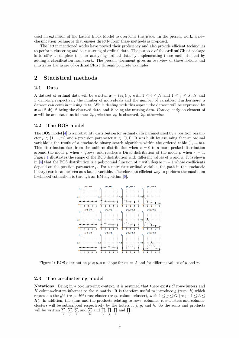
2.2 The BOS modelThe BOS model [4] is a probability distribution for ordinal data parametrized by a position param-eter µ ∈ {1, ...,m} and a precision parameter π ∈ [0, 1]. It was built by assuming that an ordinalvariable is the result of a stochastic binary search algorithm within the ordered table (1, ...,m).This distribution rises from the uniform distribution when π = 0 to a more peaked distributionaround the mode µ when π grows, and reaches a Dirac distribution at the mode µ when π = 1.Figure 1 illustrates the shape of the BOS distribution with different values of µ and π. It is shownin [4] that the BOS distribution is a polynomial function of π with degree m− 1 whose coefficientsdepend on the position parameter µ. For a univariate ordinal variable, the path in the stochasticbinary search can be seen as a latent variable. Therefore, an efficient way to perform the maximumlikelihood estimation is through an EM algorithm [6].

Figure 1: BOS distribution p(x;µ, π): shape for m = 5 and for different values of µ and π.

2.3 The co-clustering modelNotations Being in a co-clustering context, it is assumed that there exists G row-clusters andH column-clusters inherent to the x matrix. It is therefore useful to introduce g (resp. h) whichrepresents the gth (resp. hth) row-cluster (resp. column-cluster), with 1 ≤ g ≤ G (resp. 1 ≤ h ≤H). In addition, the sums and the products relating to rows, columns, row-clusters and column-clusters will be subscripted respectively by the letters i, j, g, and h. So the sums and productswill be written

∑i

,∑j

,∑g

and∑h

and∏i

,∏j

,∏g

and∏h

.

2

Latent Block Model Let consider the data matrix x = (xij)i,j . It is assumed that there existsG row-clusters and H column-clusters that correspond to a partition v = (vig)i,g and a partitionw = (wjh)j,h, with 1 ≤ g ≤ G and 1 ≤ h ≤ H. We have noted vig = 1 if i belongs to clusterg, whereas vig = 0 otherwise, and wjh = 1 when j belongs to cluster h, but wjh = 0 otherwise.Each element xij is considered to be generated under a parameterized probability density functionp(xij ;αgh). Here, g denotes the cluster of row i, and h denotes the cluster of column j, while αghrepresents the parameters of probability density function of block (g, h), a block being the crossingof both a row-cluster and a column-cluster. Figure 2 is an example of co-clustering performed onan ordinal data matrix.

Figure 2: On the left: original dataset made of ordinal data with m = 5. On the right: a co-clustering is performed with G = H = 2, the rows and columns are sorted by row-clusters andcolumn clusters, which emphasizes a structure in the dataset.

The univariate random variables xij are assumed to be conditionally independent given therow and column partitions v and w. Therefore, the conditional probability density function of xgiven v and w can be written:

p(x|v,w;α) =∏

i,j,g,h

p(xij ;αgh)vigwjh ,

where α = (αgh)g,h being the distribution’s parameters of block (g, h). Any univariate distributioncan be used in regard to the kind of data (e.g: Gaussian, Bernoulli, Poisson...). In the ordinalClustpackage, the BOS distribution is employed thus αgh = (µgh, πgh). For convenience, the label ofrow i is also denoted by vi = (vi1, ..., viG) ∈ {0, 1}G. Similarly, the label of column j is denoted bywj = (wj1, ..., wiH) ∈ {0, 1}H . These latent variables v and w are assumed to be independent sop(v,w;γ,ρ) = p(v;γ)p(w;ρ) with:

p(v;γ) =∏i,g

γvigg and p(w;ρ) =

∏j,h

ρwjh

h ,

knowing that γg = p(vig = 1) with g ∈ {1, ..., G} and ρh = p(wjh = 1) with h ∈ {1, ...,H}. Thisimplies that, for all i, the distribution of vi is the multinomial distributionM(γ1, ..., γG) and doesnot depend on i. In a similar way, for all j, the distribution of wj is the multinomial distributionM(ρ1, ..., ρH) and does not depend on j. From these considerations, the parameter of the latentblock model is defined as θ = (γ,ρ,α), with γ = (γ1, ..., γG) and ρ = (ρ1, ..., ρH) the rows andcolumns mixing proportions. Therefore, if V and W are the sets of all possible labels v and w,the probability density function p(x;θ) of x can be written:

p(x;θ) =∑

(v,w)∈V×W

∏i,g

γvigg∏j,h

ρwjh

h

∏i,j,g,h

p(xij ;αgh)vigwjh . (1)

Model Inference In the co-clustering context, the inference aim is to maximize the observedlog-likelihood l(θ; x) =

∑x

log p(x;θ). The EM-algorithm [6] is a very well known technique for

maximizing parameters with latent variables. However, regarding the co-clustering case, it is not

3

computationally tractable. Indeed, this method needs to compute the expectation of the completedata log-likelihood. Though, this expression contains the probability p(vig = 1, wjh = 1|x,θ),which needs to consider all the possible values for vi′ and wj′ with i′ 6= i and j′ 6= j. The E-stepwould require to calculate GN × HJ , With the values of the example below (G = 4, H = 4,N = 117 and J = 28) which would result in the computation of 4117 × 428 ≈ 5 × 1089 terms.There exists different alternatives to the EM algorithm as the variational EM algorithm, the SEM-Gibbs algorithm or other algorithm linked to a Bayesian inference. The SEM-Gibbs version is usedbecause it is known to avoid spurious solutions [10]. Furthermore, it handles easily missing valuesx in x, which is an important advantage, particularly with real datasets. The SEM-algorithm ismade of two iteratively repeated steps that are detailed in Algorithm 1.

Values initialization: v(0),w(0),θ(0), x(0)

for ( q in 1:(nbSEM) ){1. SE-step.1.1 Generate the row partition with v(q)ig |x, x(q−1),w(q−1) for all 1 ≤ i ≤ N , 1 ≤ g ≤ G:p(vig = 1|x(q−1),w(q−1);θ(q−1)) ∝ γ(q−1)g

∏jh

p(xij ;µ(q−1)gh , π

(q−1)gh )w

(q−1)jh .

1.2 Generate column partition with w(q)jh |x, x(q−1),v(q) for all 1 ≤ j ≤ J , 1 ≤ h ≤ H:

p(wjh = 1|x,v(q);θ(q−1)) ∝ ρ(q−1)h

∏ig

p(xij ;µ(q−1)gh , π

(q−1)gh )v

(q)ig .

1.3 Generate the missing data x(q)ij |x,v(q),w(q) as follows:

p(x(q)ij |x,v(q),w(q);θ(q−1)) =

∏g,h

p(xij ;µgh(q−1), πgh

(q−1))v(q)ig wgh

(q)

.

2. M-step.Maximization of the completed log-likelihood by updating the co-clusters BOS parameterswith an EM-algorithm (see [4] for further details).}

Algorithm 1: SEM-Gibbs for co-clustering on ordinal data.

Initialization The ordinalClust package allows two modes for values initialization, through theargument init which can take values "random" or "kmeans". The first one randomly initializes v(0)and w(0). The second one is the by default value and consists in performing a Kmeans algorithm[8] on the rows and on the columns. In both cases, θ(0) is estimated according to v(0) and w(0).Then, x(0) is sampled according to v(0), w(0) and θ(0).

Estimation of model parameters and partitions The first iterations of the SEM-Gibbs arecalled the burn-in period, which means the parameters are not stable yet. Consequently, only theiterations that occurred after this burn-in period are taken into account and are referred to assampling distribution hereafter. While the final estimation of the position parameter µgh is themode of the sampling distribution, the final estimations of the continuous parameters (πgh, γg, ρh)

are the median of the sample distribution. It leads to a final estimation of θ that is called θ. Then,a sample of (x,v,w) is generated by several SE-step (step 1. from Algorithm 1) with θ fixed toθ. The final partitions (v, w) and the missing observations x are estimated by the mode of theirsample distribution.

Model Selection To determine how many row-clusters and how many column-clusters are nec-essary, an adaptation of the ICL criterion [3] called ICL-BIC is proposed in [9]. In practice, thealgorithm has to be executed with all the (G,H) to test, and the highest ICL-BIC is retained.

2.4 The clustering modelThe clustering model described in this section is a particular case of the co-clustering model,in which each feature is in its own cluster (H = J). Consequently w is not a latent variableanymore since each variable represents a cluster of size 1. Let define a multivariate ordinal variablexi = (xij)j with 1 ≤ j ≤ J . Conditionally to cluster g, the distribution of xi is assumed to be:

4

p(xi|vig = 1;µg,πg) =∏j

p(xij ;µgj , πgj),

where µg = (µgj)j and πg = (πgj)j with 1 ≤ j ≤ J . This conditional independence hypothesisassumes that conditionally to the belonging to row-cluster g, the J ordinal responses of an indi-vidual are independently drawn from J univariate BOS models of parameters (µgj , πgj)j∈{1,...,J}.Furthermore, as in the co-clustering case, the distribution of vi is assumed to be the multinomialdistributionM(γ1, ..., γG) and not to depend on i. In this configuration, the parameter of the clus-tering model is defined as θ = (γ,α), with αgj = (µgj , πgj) being the position and precision BOSparameters of the row-cluster g and ordinal variable j. Consequently, with a matrix x = (xij)i,jof ordinal data, the probability density function p(x;θ) of x is written:

p(x;θ) =∑v∈V

∏i,g

γvigg∏i,j,g

p(xij ;µgj , πgj)vig . (2)

To infer the parameters of this model, the SEM-Gibbs Algorithm 1 is used with the 1.2 partremoved from the SE-step. The 1.3 part about missing value imputation remains as well. It ishere noticed that a clustering can be also obtained by using the co-clustering of Section 2.3, andby considering the resulting v partition as the outcome. As a matter of fact, in this case, theco-clustering is a parsimonious version of the clustering.

2.5 The classification modelBy considering a classification task with a categorical variable to predict from ordinal data, theencountered configuration is the particular case where v is known for all i ∈ {1, ..., N} and for allg ∈ {1, ..., G}. In ordinalClust, two classification models are proposed.

Multivariate BOS model This first model is similar to the clustering model: each variablerepresents a column-cluster of size 1, thus w is not a latent variable. This model assumes that,conditionally on the class of the observations, the J variables are independent. Since the rowclasses are observed, the algorithm only needs to estimate the parameter θ that maximizes thelog-likelihood l(θ; x). The probability density function p(x,v;θ) is therefore expressed as below:

p(x,v;θ) =∏i,g

γvigg∏i,j,g

p(xij ;αgj)vig . (3)

The inference of this model’s parameters only requires the M-step of Algorithm 1. However, ifthere are missing data, the SE-step made of 1.3 part only is also required.

Parsimonious BOS model This model is a parsimonious version of the first model. Parsimonyis introduced by grouping the features into H clusters (as in the co-clustering model). The mainhypothesis is that given the row-cluster partitions and the column-cluster partitions, the realizationxij is independent from the other ones. In practice the number H of column-clusters is chosenwith a training dataset and a validation dataset as follows. Consequently, the probability densityfunction p(x, v;θ) is annotated:

p(x,v;θ) =∑w∈W

∏i,g

γvigg∏j,h

ρwjh

h

∏i,j,g,h

p(xij ;αgh)vigwjh . (4)

To infer this model’s parameters, Algorithm 1 is used with an SE-step containing part 1.2 only,and the entire M-step. Again, if there are missing data, the SE-step made of 1.3 part is alsorequired.

2.6 Handling ordinal data with several numbers of levelsThe Latent Block Model as it is described before is not able to take variables with different levelsminto account. Indeed, the distributions of variables with different numbers of levels are not definedon the same support. This implies that it is impossible to gather two variables with different mwithin a same block.In [13], a constrained Latent Block Model is proposed. Although it does not make possible togather ordinal features with different m in a same column-cluster, it is able to take into account

5

the fact that there are several m and therefore to perform a co-clustering on more diverse datasets.The matrix x is considered to contain D different numbers of levels. Its representation is seen asD matrices put side by side, such that the dth table is a N × Jd matrix written xd, composed ofordinal data with numbers of levels md.

x =

x1

...

xD

, with xd = (xdij)i=1,...,N ; j=1,...,Jd and for d = 1, ..., D.

The model relies on the following hypothesis:

p(x1, ...xD|v,w1, ...,wD) = p(x1|v,w1)× ...× p(xD|v,wD),

with wd the column partition of xd. This means there is an independence between the D blocks,knowing their row and column partitions: the realization of the univariate random variable xdij willnot depend on the column partitions of the other blocks than d.

In this case, the SEM-Gibbs algorithm to infer the parameters is slightly changed: in the SE-step, a sampling step is appended to for every additional xd. For further details on this adaptedSEM-Gibbs algorithm, see [13].

3 Application on the patients quality of life analysis in on-cology

This section explains how to use the implementation of the methods described before throughordinalClust package.

3.1 DatasetsThe included datasets are taken from QoLR package [2]. They contain responses to questionnairesthat were given to patients affected by breast cancer. Furthermore, for all the questions, the mostpositive answer is given by the level “1". For example, for the question: “During the past week, didyou feel irritable?" with possible responses: “Not at all." “A little." “Quite a bit." “Very much.",the following levels number are respectively assigned to the replies: 1 “Not at all.", 2 “A little.",3 “Quite a bit.", 4 “Very much.", because it is perceived as more negative to have felt irritable.Two datasets are available:

• dataqol is a data.frame with 117 lines such that each line represents a patient and the columnscontain information about the patient:

– Id : patient Id,

– q1-q28 : responses to 28 questions with number of levels equals to 4,

– q29-q30 : responses to 2 questions with number of levels equals to 7.

• dataqol.classif is a data.frame with 40 lines such that a line represents a patient, and thecolumns contain information about the patient:

– Id : patient Id,

– q1-q28 : responses to 28 questions with number of levels equals to 4,

– q29-q30 : responses to 2 questions with number of levels equals to 7,

– death: if the patient deceased (2) or not (1).

The datasets contain missing values, that are set to 0. To load the package and its dataset, thefollowing commands must be executed:

library(ordinalClust)data("dataqol")data("dataqol.classif")

6

Then, a seed is set so that the user finds results identical to this document:

set.seed(8)

The user must define how many SEM-Gibbs iterations (nbSEM ) and how many burn-in iterations(nbSEMburn) are needed for Algorithm 1. Section 3.6 provides an empirical way of checkingrightness of these values. Moreover, the nbindmini argument has to be defined: it indicates howmany cells at least must be present in a block. At last, the init argument indicates how to initializethe algorithm. It can be set to "kmeans" or "random".

nbSEM <- 120nbSEMburn <- 80nbindmini <- 1init <- "kmeans"

3.2 Performing a classificationIn this section, the dataqol.classif dataset is used. The aim is to predict the death variable fromthe ordinal data that corresponds to the patients answers. The following snippet shows howto setup the classification configuration. First, the x ordinal data matrix (the responses to thequestionnaires) is defined, as well as the v vector, which is the variable death to predict.

x <- as.matrix(dataqol.classif[,2:29])v <- as.vector(dataqol.classif$death)

ordinalClust offers two classification models. The first one (chosen by the option kc=0 ) is amultivariate BOS model assuming that, conditionally on the class of the observations, the featuresare independent. The second model introduces parsimony by grouping the features into clustersand assuming that the features of a cluster have a common distribution. The number H of clustersof features is defined with the argument kc=H. H is chosen thanks to a training dataset and avalidation dataset:

nb.sample <- ceiling(nrow(x)*2/3)sample.train <- sample(1:nrow(x), nb.sample, replace=FALSE)x.train <- x[sample.train,]x.validation <- x[-sample.train,]v.train <- v[sample.train]v.validation <- v[-sample.train]

Then, the classification can be performed with function bosclassif and several kc parameters aretested. In the following example, the predictions matrix contains the predictions resulting fromthe classifications performed with different kc.

predictions <- matrix(0,nrow=4,ncol=nrow(x.validation))

for(kc in 0:3){res <- bosclassif(x=x.train,y=v.train, kr=2,kc=kc,m=4,

nbSEM=nbSEM,nbSEMburn=nbSEMburn,nbindmini=nbindmini, init=init)

pred <- predict(res, x.validation)predictions[(kc+1),] <- pred@zr_topredict

}

Table 1 shows the precision, recall and specificity for each different kc. The code to get thesevalues is available in Appendix. First of all, the results are globally satisfying since the precisionand recalls are pretty high. Then, it is clearly observed that the parsimonious model (when kc=1,2or 3 ) has better results than the multivariate model (kc=0 ). As a matter of fact, the mostparsimonious model with kc=3 obtains the best results. This illustrates the interest of introducingparsimonious models in a supervised context.

7

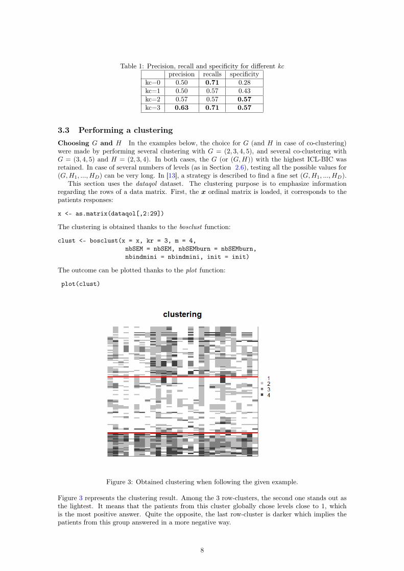
Table 1: Precision, recall and specificity for different kcprecision recalls specificity

kc=0 0.50 0.71 0.28kc=1 0.50 0.57 0.43kc=2 0.57 0.57 0.57kc=3 0.63 0.71 0.57

3.3 Performing a clusteringChoosing G and H In the examples below, the choice for G (and H in case of co-clustering)were made by performing several clustering with G = (2, 3, 4, 5), and several co-clustering withG = (3, 4, 5) and H = (2, 3, 4). In both cases, the G (or (G,H)) with the highest ICL-BIC wasretained. In case of several numbers of levels (as in Section 2.6), testing all the possible values for(G,H1, ...,HD) can be very long. In [13], a strategy is described to find a fine set (G,H1, ...,HD).

This section uses the dataqol dataset. The clustering purpose is to emphasize informationregarding the rows of a data matrix. First, the x ordinal matrix is loaded, it corresponds to thepatients responses:

x <- as.matrix(dataqol[,2:29])

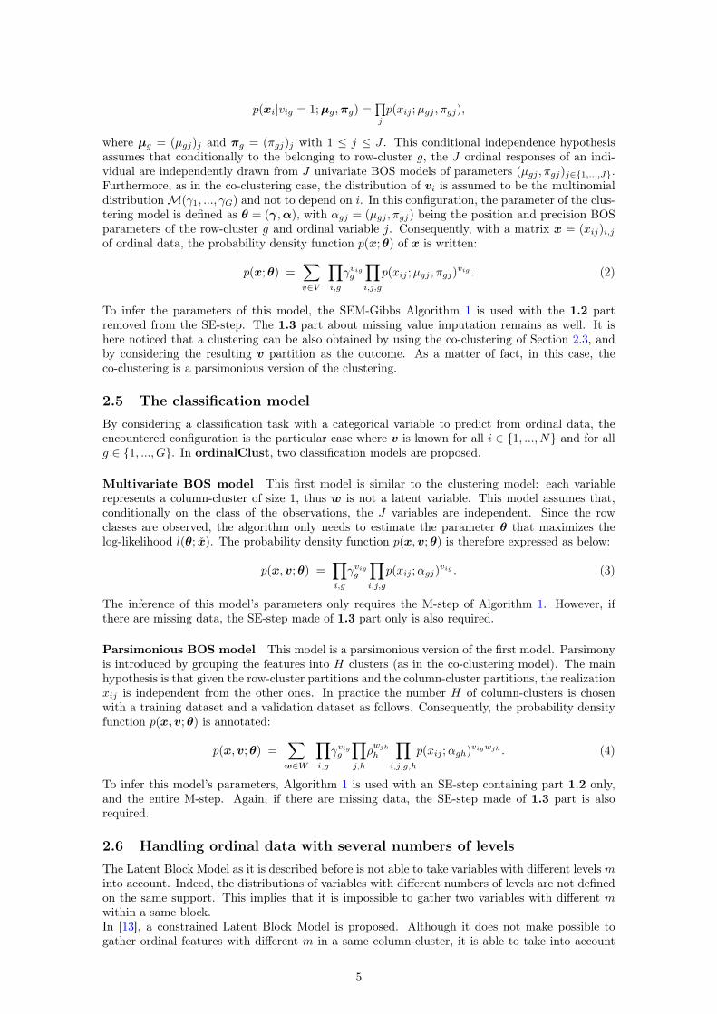
The clustering is obtained thanks to the bosclust function:

clust <- bosclust(x = x, kr = 3, m = 4,nbSEM = nbSEM, nbSEMburn = nbSEMburn,nbindmini = nbindmini, init = init)

The outcome can be plotted thanks to the plot function:

plot(clust)

Figure 3: Obtained clustering when following the given example.

Figure 3 represents the clustering result. Among the 3 row-clusters, the second one stands out asthe lightest. It means that the patients from this cluster globally chose levels close to 1, whichis the most positive answer. Quite the opposite, the last row-cluster is darker which implies thepatients from this group answered in a more negative way.

8

3.4 Performing a co-clusteringAgain, this section uses the dataqol dataset. The co-clustering is performed with the boscoclustfunction:

coclust <- boscoclust(x = x, kr = 4, kc = 4, m = 4,nbSEM = nbSEM, nbSEMburn = nbSEMburn,nbindmini = nbindmini, init = init)

As well as in the clustering context, the result can be plotted, with the command below, as inFigure 4.

plot(coclust)

Figure 4: Obtained co-clustering when following the given example.

The resulting plot is given by Figure 4. In this case, the algorithm highlights a structure amidthe rows. What’s more, it also reveals a structure inherent to the columns: for example, the fourthcolumn-cluster is lighter than the others, consequently, these questions are globally responded ina more positive way.

3.5 Comparison of clustering and co-clustering.ICL-BIC values Co-clustering can be seen as a parsimonious way of performing a clustering,that is why these two techniques are compared here. First, on a mathematical point of view, theICL-BIC of the results is available with the following command:

object@icl

In clustering, the obtained ICL-BIC is equal to −3519.776, and in co-clustering −3309.310, whichis better. Furthermore, the interpretation of row-clusters is more precise with the co-clustering.Indeed, on Figure 3, the row-clusters can be seen as a group of persons which globally repliedpositively, a group of persons which replied negatively, and a third one which replied in between.On the other hand, on Figure 4, an inherent structure of the data is better highlighted andbrings more information: for each row-cluster, it is also easy to detect the questions that werereplied negatively. Co-clustering can therefore be interpreted as a more efficient way of performingclustering.

ARI values on row partitions The Adjusted Rand Index [12] was computed on row partitionsof co-clustering and clustering results. The obtained value is 0.41, meaning that co-clusteringcreates a row partition close to clustering’s one, without being identical.

9

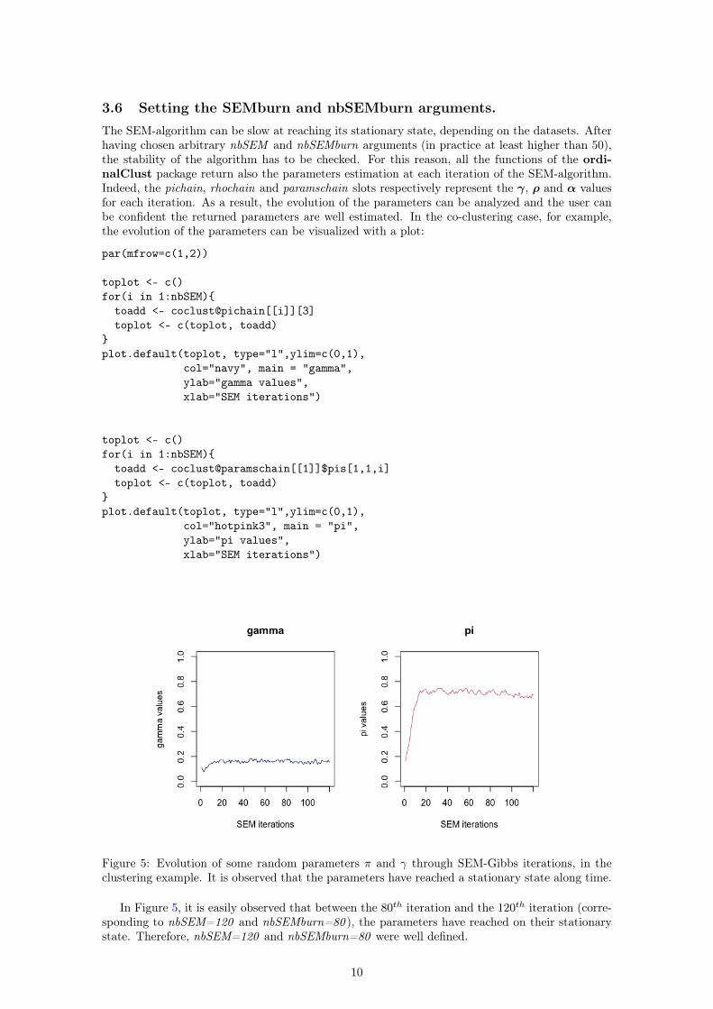
3.6 Setting the SEMburn and nbSEMburn arguments.The SEM-algorithm can be slow at reaching its stationary state, depending on the datasets. Afterhaving chosen arbitrary nbSEM and nbSEMburn arguments (in practice at least higher than 50),the stability of the algorithm has to be checked. For this reason, all the functions of the ordi-nalClust package return also the parameters estimation at each iteration of the SEM-algorithm.Indeed, the pichain, rhochain and paramschain slots respectively represent the γ, ρ and α valuesfor each iteration. As a result, the evolution of the parameters can be analyzed and the user canbe confident the returned parameters are well estimated. In the co-clustering case, for example,the evolution of the parameters can be visualized with a plot:

par(mfrow=c(1,2))

toplot <- c()for(i in 1:nbSEM){

toadd <- coclust@pichain[[i]][3]toplot <- c(toplot, toadd)

}plot.default(toplot, type="l",ylim=c(0,1),

col="navy", main = "gamma",ylab="gamma values",xlab="SEM iterations")

toplot <- c()for(i in 1:nbSEM){

toadd <- coclust@paramschain[[1]]$pis[1,1,i]toplot <- c(toplot, toadd)

}plot.default(toplot, type="l",ylim=c(0,1),

col="hotpink3", main = "pi",ylab="pi values",xlab="SEM iterations")

Figure 5: Evolution of some random parameters π and γ through SEM-Gibbs iterations, in theclustering example. It is observed that the parameters have reached a stationary state along time.

In Figure 5, it is easily observed that between the 80th iteration and the 120th iteration (corre-sponding to nbSEM=120 and nbSEMburn=80 ), the parameters have reached on their stationarystate. Therefore, nbSEM=120 and nbSEMburn=80 were well defined.

10

3.7 Handling data with different numbers of levels.If the user wants to execute one of the function described before on variables with different m,then they should use the same function but make some changes in the arguments definition. Letassume the data is made of D different number of levels. First of all, the matrix x ’s columns haveto be grouped by same number of level m[d]. The additional changes regarding the arguments topass are listed below:

• m must be vector of length D. The dth element indicates the number of levels for the dthgroup of variables.

• kc must be vector of length D. The dth element indicates the number of column-clusters forthe dth group of variables.

• idx_list is a new vector argument of length D. The dth item of the vector indicates the indexof the first column that have the number of levels m[d].

4 ConclusionThe ordinalClust package presented in this paper implements several methods for analyzingordinal data. In a first place, it proposes a co-clustering framework based on the Latent BlockModel, coupled with a SEM-Gibbs algorithm and the BOS distribution. Moreover, it presents anadaptation of these techniques to perform clustering and classification on ordinal data. For theclassification method, two models are proposed, so that the user can introduce parsimony in theiranalysis. In a similar reasoning, it has been shown that the co-clustering method actually offersa parsimonious way of performing clustering. Besides, the framework is able to handle missingvalues which is notably relevant in the case of real datasets. Finally, these techniques are alsoimplemented in the case of dataset with ordinal data having several numbers of levels.

11

References[1] Alan Agresti. Analysis of ordinal categorical data. Wiley Series in Probability and Statistics,

pages 397–405. John Wiley & Sons, Inc., 2012.

[2] Amelie Anota, Marion Savina, Caroline Bascoul-Mollevi, and Franck Bonnetain. Qolr: An rpackage for the longitudinal analysis of health-related quality of life in oncology. Journal ofStatistical Software, Articles, 77(12):1–30, 2017.

[3] Christophe Biernacki, Gilles Celeux, and Gérard Govaert. Assessing a mixture model forclustering with the integrated completed likelihood. IEEE Trans. Pattern Anal. Mach. Intell.,22(7):719–725, July 2000.

[4] Christophe Biernacki and Julien Jacques. Model-Based Clustering of Multivariate OrdinalData Relying on a Stochastic Binary Search Algorithm. Statistics and Computing, 26(5):929–943, 2016.

[5] R. H. B. Christensen. ordinal—regression models for ordinal data, 2015. R package version2015.6-28.

[6] A. P. Dempster, N. M. Laird, and D. B. Rubin. Maximum likelihood from incomplete datavia the em algorithm. Journal of he Royal Statistical Society, series B, 39(1):1–38, 1977.

[7] Gérard Govaert and Mohamed Nadif. Co-Clustering. Computing Engineering series. ISTE-Wiley, 2014.

[8] J. A. Hartigan and M. A. Wong. A k-means clustering algorithm. JSTOR: Applied Statistics,28(1):100–108, 1979.

[9] Julien Jacques and Christophe Biernacki. Model-Based Co-clustering for Ordinal Data.preprint <hal-01448299>, January 2017.

[10] Christine Keribin, Gérard Govaert, and Gilles Celeux. Estimation d’un modèle à blocs latentspar l’algorithme SEM. In 42èmes Journées de Statistique, Marseille, France, 2010.

[11] Damien McParland and Isobel Claire Gormley. Algorithms from and for Nature and Life:Classification and Data Analysis, chapter Clustering Ordinal Data via Latent Variable Models,pages 127–135. Springer International Publishing, Switzerland, 2013.

[12] William M. Rand. Objective criteria for the evaluation of clustering methods. Journal of theAmerican Statistical Association, 66(336):846–850, 1971.

[13] Margot Selosse, Julien Jacques, and Christophe Biernacki. Analyzing health quality surveyusing constrained co-clustering model for ordinal data and some dynamic implication. preprint<hal-01643910>, 2018.

[14] J.K. Vermunt and J. Magidson. Technical guide for latent gold 4.0: Basic and advanced.statistical innovations inc., 2005.

12

AppendixThe following code allows to compute the precision, recall, specificity, and sensitivity that wereobtained with the different kc, in Section 3.2

predictions = as.data.frame(predictions)row.names <- c()kcol <- c(0,1,2,3)for(kc in kcol){

name= paste0("kc=",kc)row.names <- c(row.names,name)

}rownames(predictions)=row.nameslibrary(caret)actual <- v.validation -1

precisions <- rep(0,length(kcol))recalls <- rep(0,length(kcol))specificities <- rep(0,length(kcol))for(i in 1:length(kcol)){

prediction <- unlist(as.vector(predictions[i,])) - 1conf_matrix <- table(prediction,actual)precisions[i] <- precision(conf_matrix)recalls[i] <- recall(conf_matrix)specificities[i] <- specificity(conf_matrix)

}