Package ‘orddom’February 20, 2015

Type Package

Title Ordinal Dominance Statistics

Version 3.1

Date 2013-02-04

Author Jens J. Rogmann, University of Hamburg, Department ofPsychology, Germany

Maintainer Jens J. Rogmann <Jens.Rogmann@uni-hamburg.de>

Description Computes ordinal, statistics and effect sizes as analternative to mean comparison: Cliff's delta or success ratedifference (SRD), Vargha and Delaney's A or the Area Under aReceiver Operating Characteristic Curve (AUC), the discretetype of McGraw & Wong's Common Language Effect Size (CLES) orGrissom & Kim's Probability of Superiority (PS), and the Numberneeded to treat (NNT) effect size. Moreover, comparisons toCohen's d are offered based on Huberty & Lowman's Percentage ofGroup (Non-)Overlap considerations.

Depends psych

License GPL-2

Repository CRAN

Date/Publication 2013-02-07 10:00:29

NeedsCompilation no

R topics documented:orddom-package . . . . . . . . . . . . . . . . . . . . . . . . . . . . . . . . . . . . . . 2cohd2delta . . . . . . . . . . . . . . . . . . . . . . . . . . . . . . . . . . . . . . . . . . 6delta2cohd . . . . . . . . . . . . . . . . . . . . . . . . . . . . . . . . . . . . . . . . . . 7delta_gr . . . . . . . . . . . . . . . . . . . . . . . . . . . . . . . . . . . . . . . . . . . 8dm . . . . . . . . . . . . . . . . . . . . . . . . . . . . . . . . . . . . . . . . . . . . . . 10dmes . . . . . . . . . . . . . . . . . . . . . . . . . . . . . . . . . . . . . . . . . . . . . 11dmes.boot . . . . . . . . . . . . . . . . . . . . . . . . . . . . . . . . . . . . . . . . . . 16dms . . . . . . . . . . . . . . . . . . . . . . . . . . . . . . . . . . . . . . . . . . . . . 19

1

2 orddom-package

metric_t . . . . . . . . . . . . . . . . . . . . . . . . . . . . . . . . . . . . . . . . . . . 21orddom . . . . . . . . . . . . . . . . . . . . . . . . . . . . . . . . . . . . . . . . . . . 22orddom_f . . . . . . . . . . . . . . . . . . . . . . . . . . . . . . . . . . . . . . . . . . 35orddom_p . . . . . . . . . . . . . . . . . . . . . . . . . . . . . . . . . . . . . . . . . . 37return1colmatrix . . . . . . . . . . . . . . . . . . . . . . . . . . . . . . . . . . . . . . 38

Index 40

orddom-package Ordinal Dominance Statistics

Description

This package provides ordinal, nonparametric statistics and effect sizes as an alternative to indepen-dent or paired group mean comparisons, with special reference to Cliff’s delta statistics (or successrate difference, SRD), but also providing McGraw and Wong’s common language effect size forthe discrete case (i.e. Grissom and Kim’s Probability of Superiority), Vargha and Delaney’s A (orthe Area Under a Receiver Operating Characteristic Curve AUC), and Cook & Sackett’s numberneeded to treat (NNT) effect size (cf. Kraemer & Kupfer, 2006). For the nonparametric effect sizes,various bootstrap CI estimates may also be obtained. Nonparametric effect sizes are also expressedas Cohen’s d based on percentages of group non-overlap (cf. Huberty & Lowman, 2000).

Details

Package: anRpackageType: PackageVersion: 3.1Date: 2013-02-07License: GPL-2

Note

Please cite as:

Rogmann, J. J. (2013). Ordinal Dominance Statistics (orddom): An R Project for Statistical Com-puting package to compute ordinal, nonparametric alternatives to mean comparison (Version 3.1).Available online from the CRAN website http://cran.r-project.org/.

Major changes from orddom version 3.0 to 3.1

• Correction for dmes list names

Major changes from orddom version 2.0 to 3.0

• New function dmes to easily calculate nonparametric effect size measures independently fromorddom

orddom-package 3

• Easier and more reliable input possible (vectors, lists, arrays, data frames) (by means of newfunction return1colmatrix)

• Individual variable label and test descriptions can now be assigned

• Outputs now also contain Number Needed to Treat (NNT) effect size

• (Para)metric Common Language effect size McGraw & Wong (1992) added

• Metric d CI in orddom now based on Hedges & Olkin (1985)

• Elimination of negative delta-between variance estimates for paired comparisons

• Correction of symmetric CI for independent Cliff’s delta statistics

• New function dmes.boot to calculate bootstrap-based CI for nonparametric effect size mea-sures and Cohen’s d,

• dmes.boot was largely based on R code provided by J. Ruscio and T. Mullen (2011) reusedwith kind permission

• New function delta_gr now yields a graphical and interpretational output for Cliff’s deltastatistic

• New options for one- and two-tailed CI in orddom and orddom_f, resulting in changes of rows21 and 22 of independent and rows 18 and 19 of paired orddom result matrix

• New Metric_t function (t, p and df can now be calculated and embedded in orddom as standardor Welch approximated)

Major changes from orddom Version 1.5 to 2.0

• orddom now also accepts simple vectors as x or y.

• New orddom_f() function file allows for file output of statistics for multiple sample compar-isons (e.g. csv or analyses in MS Excel or Open Office Calc).

• New orddom_p() function file allows for detailed tab-formatted output for single sample com-parisons.

• Package dependency on compute.es package was suspended (tes-Function for metric Cohen’sd in orddom).

• New metric_t() function for additional information on metric t-test results.

• The dm() function can now also return difference matrices.

• Improved stability of orddom function as well as minor corrections in orddom output andmanuals.

Major changes from orddom Version 1.0 to 1.5

• Calculation of CI and delta z-score-estimates can now be based on Students t-distributionrather than using fixed normal distribution z-scores.

• Symmetric CIs can now be obtained to increase power of the delta statistics in certain cases.

• Formulas used for calculation added in orddom manual.

4 orddom-package

• Probability of Superiority statistic as well as variance estimates for delta in the independentgroups analyses were corrected.

• Minor changes were implemented to allow for calculation of d = ±1 extreme cases withouterror abort.

• Output of raw y-dataset in independent group analysis was corrected.

• Dependencies on packages psych and compute.es declared in DESCRIPTION and NAMES-PACE files.

Author(s)

Dr. Jens J. Rogmann, University of Hamburg, Dept of Psychology, Germany Maintainer: Jens J.Rogmann <Jens.Rogmann@uni-hamburg.de>

References

Cliff, N. (1993). Dominance statistics: Ordinal analyses to answer ordinal questions. PsychologicalBulletin, 114, 494-509.

Cliff, N. (1996a). Ordinal Methods for Behavioral Data Analysis. Mahwah, NJ: Lawrence Erl-baum.

Cliff, N. (1996b). Answering ordinal questions with ordinal data using ordinal statistics. Multi-variate Behavioral Research, 31, 331-350.

Cohen, J. (1988). Statistical power analysis for the behavioral sciences (2nd edition). New York:Academic Press.

Cook, R.J. & Sackett, D. L. (1995). The number needed to treat: A clinically useful measureof treatment effect. British Medical Journal, 310, 452-454.

Delaney, H.D. & Vargha, A. (2002). Comparing Several Robust Tests of Stochastic Equality WithOrdinally Scaled Variables and Small to Moderate Sized Samples. Psychological Methods, 7, 485-503.

Feng, D., & Cliff, N. (2004). Monte Carlo Evaluation of Ordinal d with Improved ConfidenceInterval. Journal of Modern Applied Statistical Methods, 3(2), 322-332.

Feng, D. (2007). Robustness and Power of Ordinal d for Paired Data. In Shlomo S. Sawilowsky(Ed.), Real Data Analysis (pp. 163-183). Greenwich, CT : Information Age Publishing.

Grissom, R.J. (1994). Probability of the superior outcome of one treatment over another. Jour-nal of Applied Psychology, 79, 314-316.

Grissom, R.J. & Kim, J.J. (2005). Effect sizes for research. A broad practical approach. Mah-wah, NJ, USA: Erlbaum.

Huberty, C. J. & Lowman, L. L. (2000). Group overlap as a basis for effect size. Educationaland Psychological Measurement, 60, 543-563.

orddom-package 5

Kraemer, H.C. & Kupfer, D.J. (2006). Size of Treatment Effects and Their Importance to Clini-cal Research and Practice. Biological Psychiatry, 59, 990-996.

McGraw, K.O. & Wong, S.P. (1992). A common language effect size statistic. PsychologicalBulletin, 111, 361-365.

Long, J. D., Feng, D., & Cliff, N. (2003). Ordinal analysis of behavioral data. In J. Schinka &W. F. Velicer (eds.), Research Methods in Psychology. Volume 2 of Handbook of Psychology (I. B.Weiner, Editor-in-Chief). New York: John Wiley & Sons.

Romano, J., Kromrey, J. D., Coraggio, J., & Skowronek, J. (2006). Appropriate statistics for ordi-nal level data: Should we really be using t-test and Cohen’s d for evaluating group differences onthe NSSE and other surveys?. Paper presented at the annual meeting of the Florida Association ofInstitutional Research, Feb. 1-3, 2006, Cocoa Beach, Florida. Last retrieved January 2, 2012, fromwww.florida-air.org/romano06.pdf

Ruscio, J. & Mullen, T. (2012). Confidence Intervals for the Probability of Superiority Effect SizeMeasure and the Area Under a Receiver Operating Characteristic Curve. Multivariate BehavioralResearch, 47, 221-223. Vargha, A., & Delaney, H. D. (1998). The Kruskal-Wallis test and stochas-tic homogeneity. Journal of Educational and Behavioral Statistics, 23, 170-192.

Vargha, A., & Delaney, H. D. (2000). A critique and improvement of the CL common languageeffect size statistic of McGraw and Wong. Journal of Educational and Behavioral Statistics, 25,101-132.

See Also

orddom, dmes, dmes.boot and orddom_f.

Examples

## Not run:#ordinal comparison and delta statistics for independent groups x and y#(e.g. x:comparison/control group and y:treatment/experimental group)orddom(x,y,paired=FALSE)##ordinal comparison and delta statistics for paired data#(e.g. x:Pretest/Baseline and y:Posttest)orddom(x,y,paired=TRUE)##Dominance Matrix productiondms(x,y,paired=T)##Print dominance matrixorddom_p(x,y,sections="4a")##Graphic output and interpretational text for Cliff's delta statistics

6 cohd2delta

delta_gr(x,y)##nonparametric effect sizes (SRD/delta, A/AUC, CL/PS, NNT)#(e.g. C:control group scores, T:treatment group scores)dmes(C,T)##Convert Cliff's delta value to Cohen's d (as distributional non-overlap)delta2cohd(dmes(C,T)$dc)##Confidence Interval estimate of AUC (by bootstrap)#cf. Ruscio, J. & Mullen, T. (2012)#(e.g. C:control group scores, T:treatment group scores)dmes.boot(C,T,theta.es="Ac")

## End(Not run)

cohd2delta Cohen’s d to Cliff’s delta

Description

Converts Cohen’s d effect size to Cliff’s delta as non-overlap between two standard normal distri-butions

Usage

cohd2delta(d)

Arguments

d Cohen’s d value

Details

Returns delta (or non-overlap, see Table 2.2.1 in Cohen, 1988, p.22).

Value

δ(d) =2AUC(d2 )− 1

AUC(d2 )

, where AUC(x) = 1√2π

∫ x−∞ e−t

2/2 dt

Author(s)

Jens Rogmann

delta2cohd 7

References

Cohen, J. (1988). Statistical Power Analysis for the Behavioral Sciences (2nd ed.). Hillsdale, NJ,USA: Lawrence Erlbaum Associates.

See Also

delta2cohd

Examples

## Not run: > cohd2delta(1.1)[1] 0.589245> cohd2delta(2.1)[1] 0.8278607> cohd2delta(2.2)[1] 0.8430398> cohd2delta(4.0)[1] 0.9767203## End(Not run)

delta2cohd Cliff’s delta to Cohen’s d

Description

Converts Cliff’s delta estimate to Cohen’s d effect size as non-overlap between two standard normaldistributions

Usage

delta2cohd(d)

Arguments

d Cliff’s delta estimate δ.

Details

Returns Cohen’s d (or non-overlap, based on U1 in Table 2.2.1, Cohen, 1988, p.22).

Value

d(δ) = 2z −1δ−2

, where zp ≡ Φ−1(p) = AUC−1(p)

Author(s)

Jens Rogmann

8 delta_gr

References

Cohen, J. (1988). Statistical Power Analysis for the Behavioral Sciences (2nd ed.). Hillsdale, NJ,USA: Lawrence Erlbaum Associates.

See Also

cohd2delta

Examples

## Not run: > delta2cohd(-.10)[1] -0.1194342> delta2cohd(-.86)[1] -0.7725292> delta2cohd(.10)[1] 0.1320236> delta2cohd(.774)[1] 1.797902

## End(Not run)

delta_gr Cliff’s delta Graphics and Interpretation

Description

Returns a graphical representation and interpretation of Cliff’s delta

Usage

delta_gr(x,y, ... ,dv=2)

Arguments

x A 1-column matrix with optional column name containing all nx values orscores of group X or 1 (e.g. control or pretest group.).

y A 1-column matrix with optional column name containing all ny values of groupY or 2 (e.g. experimental or post-test group). For paired comparisons (e.g. pre-post), nx = ny is required.See orddom for details.

... Other arguments to be passed on to the orddom function, such as (for example):- paired: to compare dependent data (e.g. pre-post) set to paired=TRUE ,- alpha for the respective significance level to be used, e.g.alpha=.01 for 1 -onetailed to generate one-sided testing p and confidence interval (CI) values setto onetailed=TRUE ,

delta_gr 9

- studdist to obtain CI based on normal distribution z values (instead of Stu-dent distribution t) set to studdist=FALSE for 1 - symmetric to obtain symmetricrather than asymmetric CIs (see orddom for details) set to symmetric=TRUE .- onetailed for one-sided rather than the default two-tailed testing.- x.name to assign an individual label to group x (i.e. 1st or control or pretestgroup).- y.name to label the y input matrix or group y (i.e. 2nd or experimental orposttest group).- description This argument allows for assigning a string (as title or description)for the ordinal comparison outputs.

dv (For paired comparisons (dv=3) only.) Determines which ordinal δ statistics areto be returned. Set to:- dv=1 [within] to return an analysis for the nx = ny within-pair changes,- dv=2 [between] to return an analysis for the overall distribution changes, basedon all n2 − n = n(n− 1) score comparisons between y and x where i 6= j,- dv=3 [combined] to return an analysis for the combined inference dw + db. Itis advisable to use dv=3 in combination with symmetric=TRUE.

Value

Returns a graphical representation and text interpretation of Cliff’s delta.

Author(s)

Jens Rogmann

See Also

orddom

Examples

## Not run:#Paired comparison combined inference (Data taken from Long et al. (2003), Table 4)x2<-t(matrix(c(2,6,6,7,7,8,8,9,9,9,10,10,10,11,11,12,13,14,15,16),1))colnames(x2)<-c("Incidental")y2<-t(matrix(c(4,11,8,9,10,11,11,5,14,12,13,10,14,16,14,13,15,15,16,10),1))colnames(y2)<-c("Intentional")delta_gr(x2,y2,paired=TRUE,studdist=FALSE,dv=3)##Journal of Statistics Education Dataset: Oral Contraceptive Drug Interaction Study#Journal of Statistics Education, Volume 12, Number 1 (March 2004).columns<-c("SubjectNo","Seq","Period","Treatment","EEAUC","EECmax","NETAUC","NETCmax")data<-read.table("http://www.amstat.org/publications/jse/datasets/ocdrug.dat",col.names=columns)##returns delta (between) and 95x<-subset(data,data$Treatment==0)[6] #Placebo EECmax

10 dm

colnames(x)<-"Placebo Phase"y<-subset(data,data$Treatment==1)[6] #Treatment EECmaxcolnames(y)<-"Treatment Phase"delta_gr(x,y,paired=TRUE,onetailed=TRUE,dv=2)##checks treatment groups delta equivalence in placebo phase#returns delta and 95plac<-subset(data,data$Treatment==0)x<-subset(plac,plac$Period==1)[6] #control (placebo before drug)colnames(x)<-"Control (before Drug)"y<-subset(plac,plac$Period==2)[6] #experimental (placebo after drug)colnames(y)<-"Exp (Placebo after Drug)"delta_gr(x,y)#

## End(Not run)

dm Dominance or Difference Matrix Creation

Description

Returns a dominance or difference matrix based on the comparison of all values of two 1-columnmatrices x and y

Usage

dm(x, y, diff=FALSE)

Arguments

x 1 column matrix with n1 values (e.g. from group X)

y 1 column matrix with n2 values (e.g. from group Y)

diff If argument is set to true, the function will return a difference matrix. Otherwise,a dominance matrix is produced.

Details

Each difference matrix cell value dij is calculated as yj − xi across all i = 1, 2, 3, ..., n1 values(=rows) of x and i = 1, 2, 3, ..., n2 values (=rows) of y. Dominance matrix cell values are calculatedas sign(yj − xi).

Value

Returns difference or dominance matrix with X values as rownames and with Y values as column-names

dmes 11

Author(s)

Jens Rogmann

References

Cliff, N. (1996). Ordinal Methods for Behavioral Data Analysis. Mahwah, NJ: Lawrence Erlbaum.

See Also

dms

Examples

## Not run:> x<-t(matrix(c(1,1,2,2,2,3,3,3,4,5),1))> y<-t(matrix(c(1,2,3,4,4,5),1))> dm(x,y,diff=TRUE)

1 2 3 4 4 51 0 -1 -2 -3 -3 -41 0 -1 -2 -3 -3 -42 1 0 -1 -2 -2 -32 1 0 -1 -2 -2 -32 1 0 -1 -2 -2 -33 2 1 0 -1 -1 -23 2 1 0 -1 -1 -23 2 1 0 -1 -1 -24 3 2 1 0 0 -15 4 3 2 1 1 0> dm(x,y)

1 2 3 4 4 51 0 -1 -1 -1 -1 -11 0 -1 -1 -1 -1 -12 1 0 -1 -1 -1 -12 1 0 -1 -1 -1 -12 1 0 -1 -1 -1 -13 1 1 0 -1 -1 -13 1 1 0 -1 -1 -13 1 1 0 -1 -1 -14 1 1 1 0 0 -15 1 1 1 1 1 0

## End(Not run)

dmes Dominance Matrix Effect Sizes

12 dmes

Description

Generates simple list of nonparametric ordinal effect size measures such as-the Probability of Superiority (or discrete case Common Language) effect size,-the Vargha and Delaney’s A (or area under the receiver operating characteristic curve, AUC)-Cliff’s delta (or success rate difference, SRD), and -the number needed to treat (NNT) effect size(based on Cliff’s delta value).

Usage

dmes(x,y)

Arguments

x A vector or 1 column matrix with nx values from (control or pre-test or compar-ison) group X

y A vector or 1 column matrix with ny values from (treatment or post-test) groupY

Details

Based on the dominance matrix created by direct ordinal comparison of values of Y with values ofX, an associative list is returned.

Value

$nx Vector or sample size of x, nx.

$ny Vector or sample size of y, ny$PSc Discrete case Common Language CL effect size or Probability of Superiority

(PS) of all values of Y over all values of X:

PSc(Y > X) =#(yi > xj)

nynx

,where i = {1, 2, ..., ny} and j = {1, 2, ..., nx}. See orddom PS Y>X for de-tails.)

$Ac Vargha & Delaney’s A or Area under the receiver operating characteristics curve(AUC) for all possible comparisons:

A(Y > X) = [#(yi > xj) + .5(#(yi = xj)](nynx)−1

,where i = {1, 2, ..., ny} and j = {1, 2, ..., nx}. See orddom A Y>X for details.)

$dc Success rate difference when comparing all values of Y with all values of X:

dc(Y > X) =#(yi > xj)−#(yi < xj)

nynx

,where i = {1, 2, ..., ny} and j = {1, 2, ..., nx}. See orddom Cliff’s delta for

dmes 13

independent groups for details.Note that in the paired samples case with ny = nx, $dc does not return thecombined estimate, i.e. $dc 6= $dw + $db!

$NNTc Number needed to treat, based on the success rate difference or $dc−1. Seeorddom "NNT" for details.

$PSw When sample sizes are equal, this value returns the Probability of Superiority(PS) for within-changes, i.e. alle paired values: PSc(Y > X) = #(yi>xi)

nynx,

limited to the nx = ny paired cases where i = {1, 2, ..., nx = ny}. (Forunequal sample sizes, this equals $PSc.)

$Aw When sample sizes are equal, this value returns A for the paired subsamplevalues, i.e. limited to the nx = ny paired cases where i = j = {1, 2, ..., nx =ny}. (For unequal sample sizes, this equals $Ac.)

$dw When nx = ny , this value returns Cliff’s delta-within, i.e. paired comparisonslimited to the diagonal of the dominance matrix or those cases where i = j. (Forunequal sample sizes, this equals $dc.)

$NNTw Number needed to treat, based on the within-case-success rate difference or$dw−1. See orddom NNT within for dependent groups for details.

$PSb When sample sizes are equal, this gives the Probability of Superiority (PS) forall cases but within-pair changes, i.e.:

PSb(Y > X) =#(yi > xj)

nynx

,limited to those cases where i 6= j. (For unequal sample sizes, this equals $PScand $PSw.)

$Ab When sample sizes are equal, this value returns A for all cases where i 6= j. (Forunequal sample sizes, this equals $Ac.)

$db When nx = ny , this value returns Cliff’s delta-between, i.e. all but the pairedcomparisons or excepting the diagonal of the dominance matrix. The parameteris calculated by taking only those ordinal comparisons into account where i 6= j.(For unequal sample sizes, this equals $dc.)

$NNTb Number needed to treat, based on Cliff’s delta-between or $db−1. See orddomNNT between for dependent groups for details.

Author(s)

Jens J. Rogmann

References

Delaney, H.D. & Vargha, A. (2002). Comparing Several Robust Tests of Stochastic Equality WithOrdinally Scaled Variables and Small to Moderate Sized Samples. Psychological Methods, 7, 485-503.

Kraemer, H.C. & Kupfer, D.J. (2006). Size of Treatment Effects and Their Importance to Clini-cal Research and Practice. Biological Psychiatry, 59, 990-996.

14 dmes

Ruscio, J. & Mullen, T. (2012). Confidence Intervals for the Probability of Superiority Effect SizeMeasure and the Area Under a Receiver Operating Characteristic Curve. Multivariate BehavioralResearch, 47, 221-223. Vargha, A., & Delaney, H. D. (1998). The Kruskal-Wallis test and stochas-tic homogeneity. Journal of Educational and Behavioral Statistics, 23, 170-192.

Vargha, A., & Delaney, H. D. (2000). A critique and improvement of the CL common languageeffect size statistic of McGraw and Wong. Journal of Educational and Behavioral Statistics, 25,101-132.

See Also

dm, orddom

Examples

## Not run:> #Example from Efron & Tibshirani (1993, Table 2.1, p. 11)> #cf. Efron, B. & Tibshirani (1993). An Introduction to the Bootstrap. New York/London: Chapman&Hall.> y<-c(94,197,16,38,99,141,23) # Treatment Group> x<-c(52,104,146,10,50,31,40,27,46) # Control Group> dmes(x,y)$nx[1] 9

$ny[1] 7

$PSc[1] 0.5714286

$Ac[1] 0.5714286

$dc[1] 0.1428571

$NNTc[1] 7

$PSw[1] 0.5714286

$Aw[1] 0.5714286

$dw[1] 0.1428571

$NNTw

dmes 15

[1] 7

$PSb[1] 0.5714286

$Ab[1] 0.5714286

$db[1] 0.1428571

$NNTb[1] 7

> ############################################################################> #Example from Ruscio & Mullen (2012, p. 202)> #Ruscio, J. & Mullen, T. (2012). Confidence Intervals for the Probability of Superiority Effect Size Measure and the Area Under a Receiver Operating Characteristic Curve, Multivariate Behavioral Research, 47, 201-223.> x <- c(6,7,8,7,9,6,5,4,7,8,7,6,9,5,4) # Treatment Group> y <- c(4,3,5,3,6,2,2,1,6,7,4,3,2,4,3) # Control Group> dmes(y,x)$nx[1] 15

$ny[1] 15

$PSc[1] 0.8444444

$Ac[1] 0.8844444

$dc[1] 0.7688889

$NNTc[1] 1.300578

$PSw[1] 1

$Aw[1] 1

$dw[1] 1

$NNTw[1] 1

$PSb[1] 0.8333333

16 dmes.boot

$Ab[1] 0.8761905

$db[1] 0.752381

$NNTb[1] 1.329114

## End(Not run)

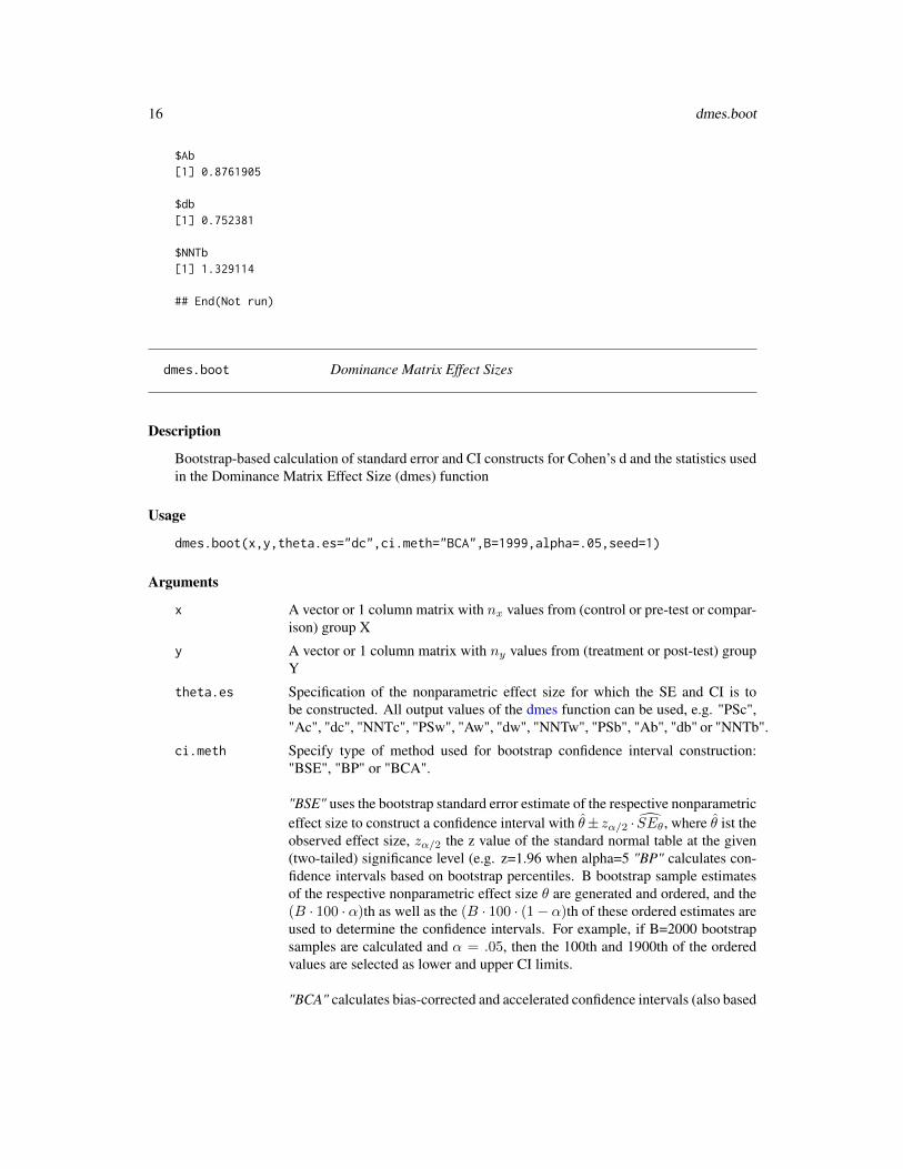
dmes.boot Dominance Matrix Effect Sizes

Description

Bootstrap-based calculation of standard error and CI constructs for Cohen’s d and the statistics usedin the Dominance Matrix Effect Size (dmes) function

Usage

dmes.boot(x,y,theta.es="dc",ci.meth="BCA",B=1999,alpha=.05,seed=1)

Arguments

x A vector or 1 column matrix with nx values from (control or pre-test or compar-ison) group X

y A vector or 1 column matrix with ny values from (treatment or post-test) groupY

theta.es Specification of the nonparametric effect size for which the SE and CI is tobe constructed. All output values of the dmes function can be used, e.g. "PSc","Ac", "dc", "NNTc", "PSw", "Aw", "dw", "NNTw", "PSb", "Ab", "db" or "NNTb".

ci.meth Specify type of method used for bootstrap confidence interval construction:"BSE", "BP" or "BCA".

"BSE" uses the bootstrap standard error estimate of the respective nonparametriceffect size to construct a confidence interval with θ± zα/2 · SEθ, where θ ist theobserved effect size, zα/2 the z value of the standard normal table at the given(two-tailed) significance level (e.g. z=1.96 when alpha=5 "BP" calculates con-fidence intervals based on bootstrap percentiles. B bootstrap sample estimatesof the respective nonparametric effect size θ are generated and ordered, and the(B · 100 · α)th as well as the (B · 100 · (1− α)th of these ordered estimates areused to determine the confidence intervals. For example, if B=2000 bootstrapsamples are calculated and α = .05, then the 100th and 1900th of the orderedvalues are selected as lower and upper CI limits.

"BCA" calculates bias-corrected and accelerated confidence intervals (also based

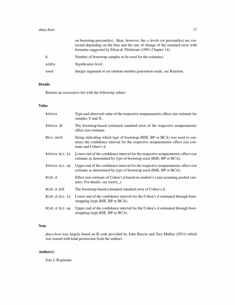
dmes.boot 17

on bootstrap percentiles). Here, however, the α levels (or percentiles) are cor-rected depending on the bias and the rate of change of the standard error withformulas suggested by Efron & Tibshirani (1993, Chapter 14).

B Number of bootstrap samples to be used for the estimates.

alpha Significance level.

seed Integer argument to set random number generation seeds, see Random.

Details

Returns an associative list with the following values:

Value

$theta Type and observed value of the respective nonparametric effect size estimate forsamples Y and X.

$theta.SE The bootstrap-based estimated standard error of the respective nonparametriceffect size estimate.

$bci.meth String indicating which type of bootstrap (BSE, BP or BCA) was used to con-struct the confidence interval for the respective nonparametric effect size esti-mate and Cohen’s d.

$theta.bci.lo Lower end of the confidence interval for the respective nonparametric effect sizeestimate as determined by type of bootstrap used (BSE, BP or BCA).

$theta.bci.up Upper end of the confidence interval for the respective nonparametric effect sizeestimate as determined by type of bootstrap used (BSE, BP or BCA).

$Coh.d Effect size estimate of Cohen’s d based on student’s t and assuming pooled vari-ance. For details, see metric_t.

$Coh.d.bSE The bootstrap-based estimated standard error of Cohen’s d.

$Coh.d.bci.lo Lower end of the confidence interval for the Cohen’s d estimated through boot-strapping (type BSE, BP or BCA).

$Coh.d.bci.up Upper end of the confidence interval for the Cohen’s d estimated through boot-strapping (type BSE, BP or BCA).

Note

dmes.boot was largely based on R code provided by John Ruscio and Tara Mullen (2011) whichwas reused with kind permission from the authors.

Author(s)

Jens J. Rogmann

18 dmes.boot

References

Efron, B. & Tibshirani (1993). An Introduction to the Bootstrap. New York/London: Chapman &Hall.

Ruscio, J. & Mullen, T. (2011). Bootstrap CI for A (R program code, last updated April 11,2011).Retrieved from http://www.tcnj.edu/~ruscio/Bootstrap%20CI%20for%20A.R .

Ruscio, J. & Mullen, T. (2012). Confidence Intervals for the Probability of Superiority Effect SizeMeasure and the Area Under a Receiver Operating Characteristic Curve. Multivariate BehavioralResearch, 47, 221-223.

See Also

dmes

Examples

## Not run:> # cf. Efron & Tibshirani (1993, Ch. 14)> # Spatial Test Data (Table 14.1, p.180)> A<-c(48,36,20,29,42,42,20,42,22,41,45,14,6,0,33,28,34,4,32,24,47,41,24,26,30,41)> B<-c(42,33,16,39,38,36,15,33,20,43,34,22,7,15,34,29,41,13,38,25,27,41,28,14,28,40)> dmes.boot(A,B)$theta

dc-0.08136095

$theta.SE[1] 0.1656658

$bci.meth[1] "BCA"

$theta.bci.lo[1] -0.4008876

$theta.bci.up[1] 0.2440828

$Coh.d[1] -0.06364221

$Coh.d.bSE[1] 0.2895718

$Coh.d.bci.lo[1] -0.6106167

$Coh.d.bci.up[1] 0.5031792

dms 19

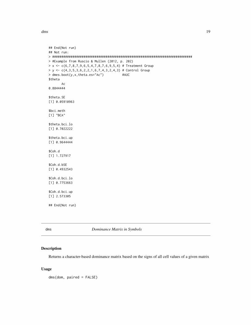
## End(Not run)## Not run:> ############################################################################> #Example from Ruscio & Mullen (2012, p. 202)> x <- c(6,7,8,7,9,6,5,4,7,8,7,6,9,5,4) # Treatment Group> y <- c(4,3,5,3,6,2,2,1,6,7,4,3,2,4,3) # Control Group> dmes.boot(y,x,theta.es="Ac") #AUC$theta

Ac0.8844444

$theta.SE[1] 0.05910963

$bci.meth[1] "BCA"

$theta.bci.lo[1] 0.7022222

$theta.bci.up[1] 0.9644444

$Coh.d[1] 1.727917

$Coh.d.bSE[1] 0.4932543

$Coh.d.bci.lo[1] 0.7753663

$Coh.d.bci.up[1] 2.573305

## End(Not run)

dms Dominance Matrix in Symbols

Description

Returns a character-based dominance matrix based on the signs of all cell values of a given matrix

Usage

dms(dom, paired = FALSE)

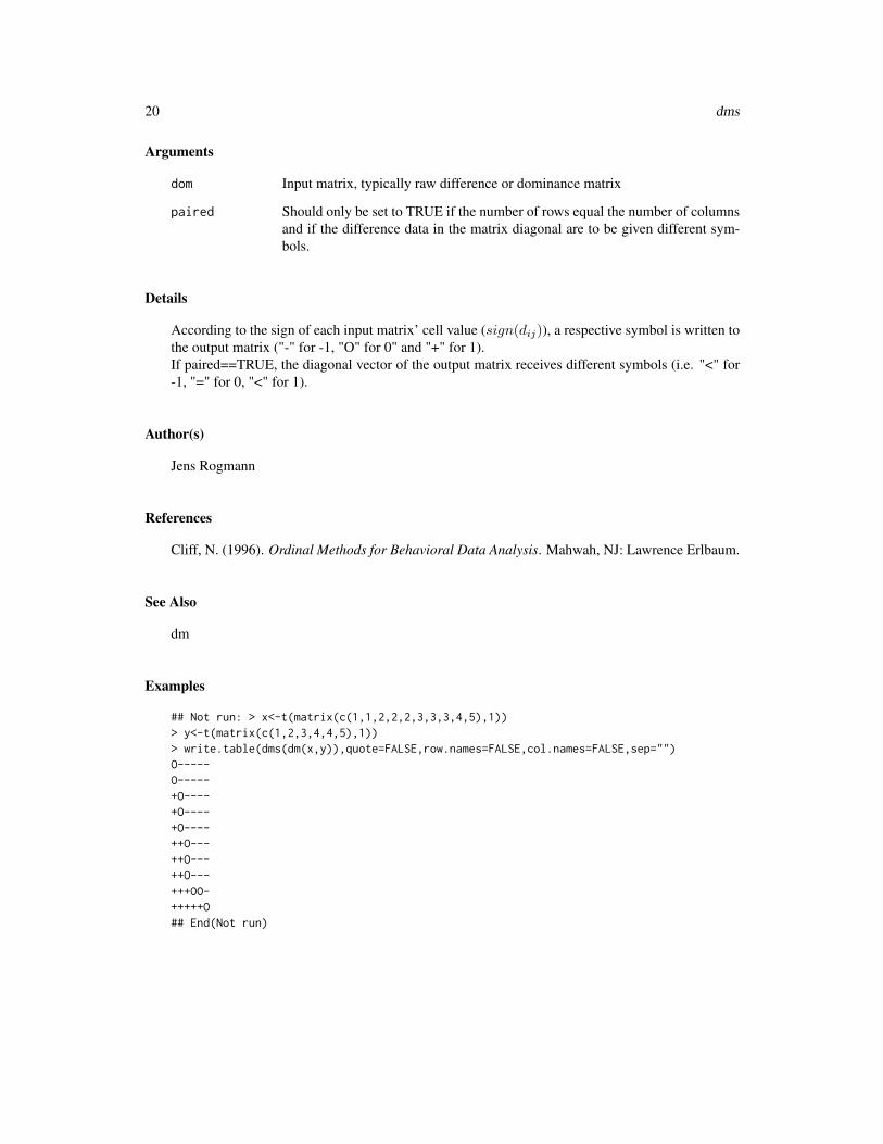
20 dms

Arguments

dom Input matrix, typically raw difference or dominance matrix

paired Should only be set to TRUE if the number of rows equal the number of columnsand if the difference data in the matrix diagonal are to be given different sym-bols.

Details

According to the sign of each input matrix’ cell value (sign(dij)), a respective symbol is written tothe output matrix ("-" for -1, "O" for 0" and "+" for 1).If paired==TRUE, the diagonal vector of the output matrix receives different symbols (i.e. "<" for-1, "=" for 0, "<" for 1).

Author(s)

Jens Rogmann

References

Cliff, N. (1996). Ordinal Methods for Behavioral Data Analysis. Mahwah, NJ: Lawrence Erlbaum.

See Also

dm

Examples

## Not run: > x<-t(matrix(c(1,1,2,2,2,3,3,3,4,5),1))> y<-t(matrix(c(1,2,3,4,4,5),1))> write.table(dms(dm(x,y)),quote=FALSE,row.names=FALSE,col.names=FALSE,sep="")O-----O-----+O----+O----+O----++O---++O---++O---+++OO-+++++O## End(Not run)

metric_t 21

metric_t Metric t-test parameters matrix

Description

Returns a matrix of independent or paired t-test data for comparison to ordinal alternatives

Usage

metric_t(a,b,alpha=0.05,paired=FALSE,t.welch=TRUE)

Arguments

a First dataset (vector or matrix).

b Second dataset (vector or matrix).

alpha Significance or α-level used for the calculation of the confidence intervals. De-fault value is α = .05 or 5 Percent.

paired By default, independence of the two groups or data sets is assumed. If thenumber of cases in x and y are equal and paired (e.g. pre-post) comparisons,this should be set to TRUE.

t.welch By default, the variances of the two datasets are not assumed equal. If the pooledvariance is needed for t, p, and df this should be set to FALSE. This setting hasno effect on the calculation of Cohens’d.

Value[1,1] or ["Diff M" ,1]

Mean Difference y − x or estimate (in the paired case) See t.test for details.[2,1] or ["t value" ,1] or ["t(dep.)" ,1]

Value of the t-statistic for the independent or the paired case. See t.test fordetails.

[3,1] or ["df" ,1] or ["df" ,1]

Degrees of freedom for the t-statistic. For independent samples, the Welch ap-proximation of degrees of freedom is returned unless t.welch is set to FALSE.See t.test for details.

[4,1] or ["p value" ,1]

The p-value of the test. See t.test for details. For independent samples, theWelch approximation of degrees of freedom is returned unless t.welch is set toFALSE.

[5,1] or ["Cohen’s d" ,1]

Cohen’s d effect size for both the independent and the paired case calculatedusing student’s t (i.e. assuming pooled variance) as

dCohen = t(pooledvar)

√ny + nxnynx

,

22 orddom

following the advice of Dunlap, Cortina, Vaslow and Burke (1996) who sug-gested using the independent group t-value and the original standard deviationsalso for the paired case to avoid overestimation of the effect size.

Author(s)

Jens J. Rogmann, University of Hamburg, Department of Psychology,Hamburg, Germany (Jens.Rogmann@uni-hamburg.de)

References

Dunlap, W. P., Cortina, J. M., Vaslow, J. B., & Burke, M. J. (1996). Meta-analysis of experimentswith matched groups or repeated measures designs. Psychological Methods, 1, 170-177.

See Also

t.test

Examples

## Not run:> #Example from Dunlap et al. (1996), Table 1> y<-c(27,25,30,29,30,33,31,35)> x<-c(21,25,23,26,27,26,29,31)> metric_t(x,y)

[,1]Diff M 4.00000000t value 2.52982213df Welch 14.00000000p value 0.02403926Cohen's d 1.26491106> metric_t(x,y,paired=TRUE)

[,1]Diff M 4.000000000t(dep.) 4.512608599df 7.000000000p value 0.002756406Cohen's d 1.264911064

## End(Not run)

orddom Ordinal Dominance Statistics

Description

Returns an array of ordinal dominance statistics based on the input of two 1-column matrices as analternative to independent or paired group mean comparisons (especially for Cliff’s delta statistics).

orddom 23

Usage

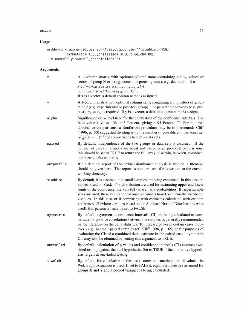
orddom(x,y,alpha=.05,paired=FALSE,outputfile="",studdist=TRUE,symmetric=FALSE,onetailed=FALSE,t.welch=TRUE,

x.name="",y.name="",description="")

Arguments

x A 1-column matrix with optional column name containing all nx values orscores of group X or 1 (e.g. control or pretest group.), e.g. declared in R asx<-t(matrix(c(x1, x2, x3, x4, . . . , xnx ),1))colnames(x)<-c("[label of group X]").If x is a vector, a default column name is assigned.

y A 1-column matrix with optional column name containing all ny values of groupY or 2 (e.g. experimental or post-test group). For paired comparisons (e.g. pre-post), nx = ny is required. If y is a vector, a default column name is assigned.

alpha Significance or α-level used for the calculation of the confidence intervals. De-fault value is α = .05 or 5 Percent, giving a 95 Percent CI. For multipledominance comparisons, a Bonferroni procedure may be implemented: Cliff(1996, p.150) suggested dividing α by the number of possible comparisons, i.e.α( 1

2k(k − 1))−1 for comparisons beteen k data sets.

paired By default, independence of the two groups or data sets is assumed. If thenumber of cases in x and y are equal and paired (e.g. pre-post) comparisons,this should be set to TRUE to return the full array of within, between, combinedand metric delta statistics.

outputfile If a a detailed report of the ordinal dominance analysis is wanted, a filenameshould be given here. The report as standard text file is written to the currentworking directory.

studdist By default, it is assumed that small samples are being examined. In this case, z-values based on Student’s t-distribution are used for estimating upper and lowerlimits of the confidence intervals (CI) as well as z-probabilities. If larger samplesizes are used, these values approximate estimates based on normally distributedz-values. In this case or if comparing with estimates calculated with orddomversions <1.5 (where z-values based on the Standard Normal Distributions wereused), this parameter may be set to FALSE.

symmetric By default, asymmetric confidence intervals (CI) are being calculated to com-pensate for positive correlations between the samples as generally recommendedby the literature on the delta statistics. To increase power in certain cases, how-ever - e.g. in small paired samples (cf. Cliff 1996, p. 165) or fur purposes ofevaluating the CIs of a combined delta estimate in the paired case - symmetricCIs may also be obtained by setting this argument to TRUE.

onetailed By default, calculation of p values and confidence intervals (CI) assumes two-sided testing against the null hypothesis. Set to TRUE if the alternative hypoth-esis targets at one-tailed testing.

t.welch By default, for calculation of the t-test scores and metric p and df values, theWelch approximation is used. If set to FALSE, equal variances are assumed forgroups X and Y and a pooled variance is being calculated.

24 orddom

x.name By default, the label of group x (i.e. 1st or control or pretest group) is taken fromthe column name of the x input matrix. This argument allows for assigning analternative label.

y.name This argument allows for assigning an alternative label for the y input matrix orgroup y (i.e. 2nd or experimental or posttest group).

description This argument allows for assigning a string (as title or description) for the ordi-nal comparison outputs.

Value

INDEPENDENT GROUPS (paired argument set to FALSE)

In the case of independent groups or data sets X and Y (e.g. comparison group X vs. treatmentgroup Y), a 2-column-matrix containing 29 rows with values is returned.

The ordinal statistics can be retrieved from the first column (named "ordinal") while the secondcolumn (named "metric") contains metric comparison data where appropriate.

[1 or ["var1_X", col#]

Label assigned to group x (x.name or column name of the x input matrix) or adefault "1st var (x)".

[2 or ["var2_Y", col#]

Label assigned to group x (x.name or column name of the x input matrix) or adefault "2nd var (y)".

[3 or ["type_title", col#]

Column 1: Returns type of the comparison, in this case "indep".Column2: In case a string header is defined by use of the comp.name argument,it is returned in column 2.

[4 or ["n in X", col#]

Number of cases in x (i.e. group X sample size).

[5 or ["n in Y", col#]

Number of cases in y (i.e. group Y sample size).

[6 or ["N #Y>X", col#]

Number of occurences of an observation from group y having a higher valuethan an observation from group x when comparing all x scores with all y scores:N#Y >X = #(yi > xj), where \# denotes "the number of times" whilst com-paring each i = 1, 2, 3, . . . ny score in sample Y with each j = 1, 2, 3, . . . nxscore in sample X (resulting in nx·ny comparisons).

[7 or ["N #Y=X", col#]

Number of occurences of an observation from group y having the same value asan observation from group x: N#Y=X = #(yi = xj).

orddom 25

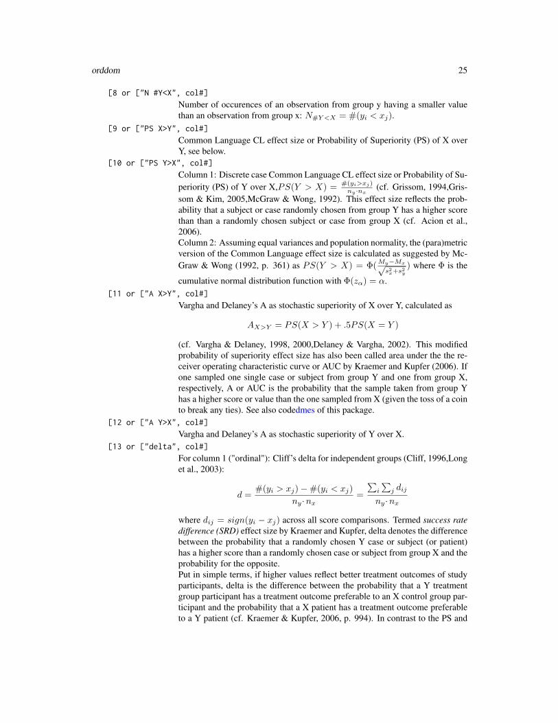
[8 or ["N #Y<X", col#]

Number of occurences of an observation from group y having a smaller valuethan an observation from group x: N#Y <X = #(yi < xj).

[9 or ["PS X>Y", col#]

Common Language CL effect size or Probability of Superiority (PS) of X overY, see below.

[10 or ["PS Y>X", col#]

Column 1: Discrete case Common Language CL effect size or Probability of Su-periority (PS) of Y over X,PS(Y > X) =

#(yi>xj)ny·nx (cf. Grissom, 1994,Gris-

som & Kim, 2005,McGraw & Wong, 1992). This effect size reflects the prob-ability that a subject or case randomly chosen from group Y has a higher scorethan than a randomly chosen subject or case from group X (cf. Acion et al.,2006).Column 2: Assuming equal variances and population normality, the (para)metricversion of the Common Language effect size is calculated as suggested by Mc-Graw & Wong (1992, p. 361) as PS(Y > X) = Φ(

My−Mx√s2x+s

2y

) where Φ is the

cumulative normal distribution function with Φ(zα) = α.[11 or ["A X>Y", col#]

Vargha and Delaney’s A as stochastic superiority of X over Y, calculated as

AX>Y = PS(X > Y ) + .5PS(X = Y )

(cf. Vargha & Delaney, 1998, 2000,Delaney & Vargha, 2002). This modifiedprobability of superiority effect size has also been called area under the the re-ceiver operating characteristic curve or AUC by Kraemer and Kupfer (2006). Ifone sampled one single case or subject from group Y and one from group X,respectively, A or AUC is the probability that the sample taken from group Yhas a higher score or value than the one sampled from X (given the toss of a cointo break any ties). See also codedmes of this package.

[12 or ["A Y>X", col#]

Vargha and Delaney’s A as stochastic superiority of Y over X.[13 or ["delta", col#]

For column 1 ("ordinal"): Cliff’s delta for independent groups (Cliff, 1996,Longet al., 2003):

d =#(yi > xj)−#(yi < xj)

ny·nx=

∑i

∑j dij

ny·nx

where dij = sign(yi − xj) across all score comparisons. Termed success ratedifference (SRD) effect size by Kraemer and Kupfer, delta denotes the differencebetween the probability that a randomly chosen Y case or subject (or patient)has a higher score than a randomly chosen case or subject from group X and theprobability for the opposite.Put in simple terms, if higher values reflect better treatment outcomes of studyparticipants, delta is the difference between the probability that a Y treatmentgroup participant has a treatment outcome preferable to an X control group par-ticipant and the probability that a X patient has a treatment outcome preferableto a Y patient (cf. Kraemer & Kupfer, 2006, p. 994). In contrast to the PS and

26 orddom

A effect sizes, delta thus takes potentially worse or harmful treatment outcomesinto account.

In column 2, the metric differences between the means are given: y − x = dijbetween all comparable x and y scores with dij = yi − xj .

[14 or ["1-alpha", col#]

Significance or α-level for CI estimation, given as percentage between 0 and100.

[15 or ["CI low", col#]

Unless the default symmetric parameter is explicitly set to TRUE, improved for-mulas are used (Feng & Cliff, 2004) to caculate asymmetric confidence interval(CI) boundary estimates of delta or mean difference:

CIlower/upper =d− d3 ± tα/2sd

√1− 2d2 + d4 + t2α/2s

2d)

1− d2 + t2α/2s2d

,

with t-values at the given α-level taken from Student’s t distribution by default(unless the studdist is set FALSE, in which case t-values are based on z-valuesfrom the Standard Normal Distribution ).

In case the symmetric argument is explicitly set to TRUE, however, ordinaryCIs are being calculated with CIlower/upper = d± tα/2sd.

In any case, if Cliffs’ d = ±1, one CI is assumed being equal to d, the respectiveother is calculated as

CIlower/upper = ((nb − t2α/2))(nb + t2α/2)−1,

where tα/2 is the t-value or z-score at the selected α level (2-tailed) of the re-spective studdist-controlled distribution, and nb the number of observations orcases in the smaller of the two samples.

[16 or ["CI high", col#]

Confidence interval upper boundary estimate of delta or mean difference.[17 or ["s delta", col#]

Unbiased sample estimate of the delta standard deviation in column 1.In column 2 ("metric"): Pooled standard deviation of metric mean differencewith sxy = [((nx − 1)sx + (ny − 1)sy)/(nx + ny − 2)]1/2 .

[18 or ["var delta", col#]

Column 1: Variance of delta (unbiased sample estimate), calculated as

s2d =n2y∑

(di· − d)2 + n2x∑

(d·j − d)2 −∑∑

(dij − d)2

nxny(nx − 1)(ny − 1),

or, using the partial variances

s2d =n2y(nx − 1)s2di· + n2x(ny − 1)s2d·j − (nxny − 1)s2dij

nxny(nx − 1)(ny − 1),

orddom 27

which can also alternatively be put as

s2d =nys

2di·

nx(ny − 1)+

nxs2d·j

ny(nx − 1)−

(nxny − 1)s2dijnxny(nx − 1)(ny − 1)

.

(For differences to Cliff’s (1996, p. 138) formula see notes to Row 28 ("var dij")below.)

In case this calculation of s2d yields values of less than (1−d2)/(nxny−1), thislatter formula is used for calculating the variance of delta.

Column 2 contains the pooled s2xy .

[19 or ["se delta", col#]

Column 2 only: metric Standard error of mean difference:SExy = sxy

√1/nx + 1/ny .

[20 or ["z/t score", col#]

Column 1: z score of delta on the of the respective studdist-controlled distribu-tion (Student’s t or standard normal).

Column 2: Metric z/t-score (= dij/SExy). In the metric case, the t.welch de-cides upon assumption of equal variances for X and Y.

[21 or ["H1 tails p/CI", col#]

Equals 1 for one-tailed and 2 for two-tailed testing of alternative or H_1-hypothesis,affecting CI and p values.

[22 or ["p", col#]

Probability of z/t score (1-sided or 2-sided comparison as shown in row 21).

[23 or ["Cohen’s d", col#]

Cohen’s d effect size estimate of delta. For Cliff’s delta inferred from distribu-tional non-overlap as suggested by Grissom & Kim (2005, p. 106 f.) as wellas Romano, Kromrey, Coraggio, & Skowronek (2006, p. 14-15), relating to therelative positions of the distributions of X and Y. When Cliff’s delta equals 0,there is no effect, and the Y and X distributions overlap completely. If there areeffects, a certain percentage of non-overlap between X and Y is created, and therelative positions of the X and Y distribtions shift. The degree of non-overlapthus is a measure of effect size and is expressed as Cohen’s d in terms of non-overlap between two normal distributions (based on U1 in Table 2.2.1, Cohen,1988, p.22). See delta2cohd manual of orddom package.Column 2 returns Cohen’s d assuming a pooled variance for t. See metric_t fordetails.

[24 or ["d CI low", col#]

Column 1: Cohen’s d effect size estimate of the lower boundary of confidenceinterval (row 15) by using the non-overlap strategy.Column 2: Confidence bands for metric Cohen’s d are constructed based onthe estimated standard deviation of Cohen’s d’s theoretical sampling distribu-tion, assuming asymptotic normality (Hedges & Olkin, 1985), calculated asCIlower/upper = d ± zsd, where z is the z-score at the selected α level (2-

28 orddom

tailed) of the standard normal distribution, and

sd =

√nx + nynxny

+d2

2(nx + ny)

.[25 or ["d CI high", col#]

Column 1:Cohen’s d estimate of upper boundary of confidence interval (row16).Column 2: see row 24 for details.

[26 or ["var d.i", col#]

Row variance of dominance/difference matrix, calculated as(nx − 1)−1

∑(di· − d)2. The metric descriptive in column 2 is the variance of

x (or s2x).[27 or ["var dj.", col#]

Column variance of dominance/difference matrix, calculated as(ny − 1)−1

∑(d·j − d)2. The metric descriptive in column 2 is the variance of

y (or s2y).

[28 or ["var dij", col#]

Variance of dominance/difference matrix as sample estimate according to Longet al. (2003, section 3.3 before eqn. 67):

s2dij =

∑∑(dij − d)2

nxny − 1=

∑d2ij −

(∑

dij)2

nxny

nxny − 1,

thus avoiding Cliff’s original (1996, p. 138) suggestion to use (nx− 1)(ny − 1)as the denominator).

[29 or ["df", col#]

If the studdist parameter is not set to FALSE, column 1 returns the degrees offreedom (df ) used for CI as well as z/t-score and z-probability estimates.In column 2 ("metric") df as used for metric t-test.

[30 or ["NNT", col#]

The number needed to treat effect size (NNT, cf. Cook & Sackett, 1995) isreturned based on the delta statistic as

delta−1

as suggested by Kraemer & Kupfer, 2006, p. 994.In column 2, the NNT is returned based on Cohen’s d of the metric between-group comparison.

orddom 29

DEPENDENT/PAIRED GROUPS (paired argument set to TRUE)

In the case of paired data (e.g. pretest-posttest comparisons of the nx = ny same subjects), a4-column-matrix containing 29 rows with values is returned.

The ordinal statistics for dij can be retrieved from the first three columns (named

within [.,1] for the nx = ny within-pair changes (where i = j in all cases);

between [.,2] for the overall distribution changes, based on all n2−n = n(n−1) comparisonswhere i 6= j,and

combined [.,3] for combined inferences dw + db.

Here, the fourth column (named "metric") contains metric comparison data.

[1 or ["var1_X_pre", col#]

Original column name of the x (or pretest) input matrix.[2 or ["var2_Y_post", col#]

Original column name of the y (or posttest) input matrix.[3 or ["type_title", col#]

Columns 1-3: Return type of the comparison, in this case "paired".Column4: In case a string header is defined by use of the comp.name argument,it is returned in column 4.

[4 or ["N #Y>X", col#]

Number of occurences (\#) of a posttest observation yi having a higher valuethan a pretest observation xj : N#Y >X = #(yi > xj), limited to the respectivepairs under observation in within, between or combined.Column 4 equals column 3.

[5 or ["N #Y=X", col#]

Number of occurences of a posttest observation having the same value as apretest observation, limited to the respective pairs under observation in within,between or combined.Column 4 equals column 3.

[6 or ["N #Y<X", col#]

Number of occurences of a posttest observation having a smaller value than apretest observation, limited to the respective pairs under observation in within,between or combined.Column 4 equals column 3.

[7 or ["PS X>Y", col#]

Common Language CL effect size or Probability of Superiority (PS) of X overY (Grissom, 1994,Grissom & Kim, 2005) (limited to the respective pairs underobservation in within, between or combined):

PS(Y > X) =#(yi > xj)

ny·nx.

30 orddom

. This effect size reflects the probability that a subject or case randomly chosenfrom the X- or pre-test-scores under observation has a higher score than than arandomly chosen case from the respective Y- or post-test-subsample (cf. Acionet al., 2006).Column 4: Assuming equal variances and population normality, the (para)metricversion of the Common Language effect size is calculated as suggested by Mc-Graw & Wong (1992, p. 363) for correlated samples by using the variancesum law to adjust the variance on the difference scores with PS(Y > X) =

Φ(My−Mx√

s2x+s2y−2rxysxsy

) where Φ is the cumulative normal distribution function

with Φ(zα) = α.[8 or ["PS Y>X", col#]

Common Language CL effect size or Probability of Superiority (PS) of Y overX (Grissom, 1994,Grissom & Kim, 2005) (limited to the respective pairs underobservation in within, between or combined).Column 4: CL (para)metric version for the correlated samples case (see row 7above for details on calculation).

[9 or ["A X>Y", col#]

Vargha and Delaney’s A as stochastic superiority of X over Y, limited to the re-spective pairs under observation in within, between or combined. (See codedmesof this orddom package for details.)Column 4 equals column 3.

[10 or ["A Y>X", col#]

Vargha and Delaney’s A as stochastic superiority of Y over X, limited to the re-spective pairs under observation in within, between or combined. (See codedmesof this orddom package for details.)Column 4 equals column 3.

[11 or ["delta", col#]

For columns 1 to 3 ("ordinal"), the respective delta for dependent groups (Cliff,1996,Long et al., 2003,Feng, 2007) is reported. With dij = sign(yi − xj),

Column 1 reports the (within) value, which is the "difference between the pro-portion of individual subjects who change in one direction and the proportion ofindividuals who change in the other" (Cliff, 1996, p. 159), calculated as

dw = (∑i =

∑j

dii)/n,

where i = j in the n = nx = ny possible paired comparisons.

"The extent to which the overall distribution has moved, except for the self-comparisons" (Cliff, 1996, p. 160) is given in column 2, the delta-(between)statistic. It is estimated by the average between-subject dominance, calculatedas

db = (∑i 6=

∑j

dij)/(n(n− 1)),

where i 6= j.

orddom 31

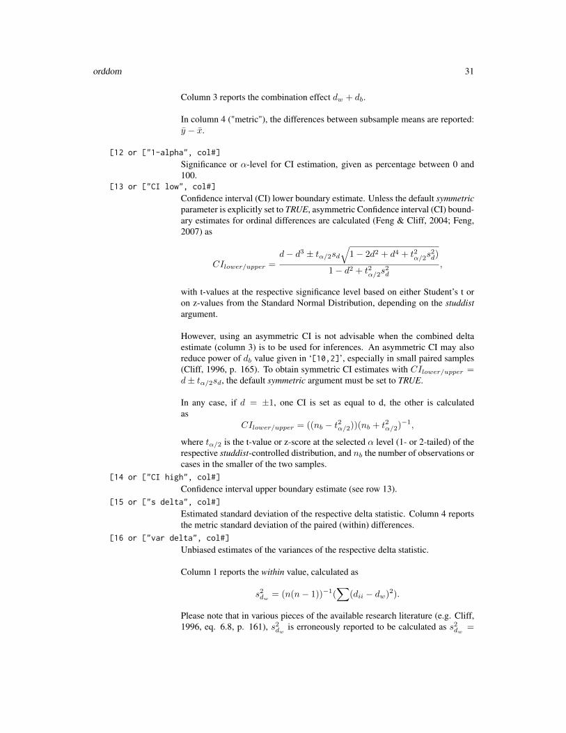
Column 3 reports the combination effect dw + db.

In column 4 ("metric"), the differences between subsample means are reported:y − x.

[12 or ["1-alpha", col#]

Significance or α-level for CI estimation, given as percentage between 0 and100.

[13 or ["CI low", col#]

Confidence interval (CI) lower boundary estimate. Unless the default symmetricparameter is explicitly set to TRUE, asymmetric Confidence interval (CI) bound-ary estimates for ordinal differences are calculated (Feng & Cliff, 2004; Feng,2007) as

CIlower/upper =d− d3 ± tα/2sd

√1− 2d2 + d4 + t2α/2s

2d)

1− d2 + t2α/2s2d

,

with t-values at the respective significance level based on either Student’s t oron z-values from the Standard Normal Distribution, depending on the studdistargument.

However, using an asymmetric CI is not advisable when the combined deltaestimate (column 3) is to be used for inferences. An asymmetric CI may alsoreduce power of db value given in ‘[10,2]’, especially in small paired samples(Cliff, 1996, p. 165). To obtain symmetric CI estimates with CIlower/upper =d± tα/2sd, the default symmetric argument must be set to TRUE.

In any case, if d = ±1, one CI is set as equal to d, the other is calculatedas

CIlower/upper = ((nb − t2α/2))(nb + t2α/2)−1,

where tα/2 is the t-value or z-score at the selected α level (1- or 2-tailed) of therespective studdist-controlled distribution, and nb the number of observations orcases in the smaller of the two samples.

[14 or ["CI high", col#]

Confidence interval upper boundary estimate (see row 13).[15 or ["s delta", col#]

Estimated standard deviation of the respective delta statistic. Column 4 reportsthe metric standard deviation of the paired (within) differences.

[16 or ["var delta", col#]

Unbiased estimates of the variances of the respective delta statistic.

Column 1 reports the within value, calculated as

s2dw = (n(n− 1))−1(∑

(dii − dw)2).

Please note that in various pieces of the available research literature (e.g. Cliff,1996, eq. 6.8, p. 161), s2dw is erroneously reported to be calculated as s2dw =

32 orddom

(n − 1)−1(∑

(dii − dw)2). The denominator, however must read n(n − 1) as"using just (n − 1) would give the variance of the individual dii whereas wewant the variance of dw, which is a kind of mean" (Feng, 07.02.2011, personalcommunication).

The (between) unbiased estimate in column 2 is calculated ass2db = [(n− 1)2(

∑(di· − db)2 +

∑(d·j − db)2 + 2

∑(di· − db)(d·j − db))−∑∑

(dij − db)2 −

∑∑(dij − db)(dji − db)][n(n − 1)(n − 2)(n − 3)]−1.

In case this formula renderes negative variance estimates for s2db estimates byuse of this formula, the between variance is alternatively calculated as s2db =(1 − d2b)/(n2 − n − 1) (see Long et al. (2003, par after eqn. 66) for a relateddiscussion).

Since dw and db are interdependent, the combined effect involves taking intoaccount their estimated covariance when calculating the unbiased estimate forthe variance for the sum of dw and db, which is reported in column 3 ass2dw+db

= s2dw + s2db + 2cov(db, dw), with

cov(db, dw) =(∑

i[dii(∑j(dij) +

∑j(dji)]− 2n(n− 1)dbdw

)(n(n−1)(n−

2))−1.

Column 4 reports the metric variance of the paired (within) differences.

[17 or ["z/t score", col#]

z score of delta. In column 4 ("metric") equal to the t-test score (assuming equalvariances).

[18 or ["H1 tails p/CI", col#]

Equals 1 for one-tailed and 2 for two-tailed testing of alternative or H_1-hypothesis,affecting CI and p values.

[19 or ["p", col#]

Probability of z-score (1 or 2-tailed comparison as shown in row 18).

[20 or ["Cohen’s d", col#]

Cohen’s d estimate of the respective delta value (see above). In the metric case,the between group t-value and the original standard deviations are also used forthe paired case to avoid overestimation of the effect size (Dunlap et al., 1996).See delta2cohd for details.Not available for the combined delta in column 3.

[21 or ["d CI low", col#]

Column 1 and 2: Cohen’s d estimate of lower boundary of the respective confi-dence interval (row 13) by using the non-overlap calculation strategy.Column 3: Not available.Column 4: Confidence bands for metric Cohen’s d are constructed based onthe estimated standard deviation of Cohen’s d’s theoretical sampling distribu-tion, assuming asymptotic normality (Hedges & Olkin, 1985), calculated asCIlower/upper = d ± zsd, where z is the z-score at the selected α level (2-

orddom 33

tailed) of the standard normal distribution, and

sd =

√nx + nynxny

+d2

2(nx + ny)

.[22 or ["d CI high", col#]

Cohen’s d estimate of upper boundary of the respective confidence interval (seerow 21 for calculation details).

[23,3] or ["var d.i",combined]

Component of s2dw+db: s2di. (Available for the combined analyses in column 3

only.) The metric descriptive in column 4 is the variance of x (or s2x.

[24,3] or ["var dj.",combined]

Component of s2dw+db: s2d.i (Third column only.) The metric descriptive in

column 4 is the variance of y (or s2y .

[25,3] or ["cov(di,dj)",combined]

Component of s2dw+db: cov(di., d.j) (Third column only.)

[26,3] or ["var dij",combined]

Component of s2dw+db: s2dij (Third column only.)

[27,3] or ["cov(dih,dhi)",combined]

Component of s2dw+db: cov(dih, dhi) (Third column only.)

[28,3] or ["cov(db,dw)",combined]

Estimated covariance between db and dw: cov(db, dw) (for purposes of com-bined inferences). (Third column only.)

[29 or ["df", col#]

Unless the studdist argument is not set to FALSE, the degrees of Freedom dfused for the CI and z-score calculations are reported in column 1.

Column 2 returns the df used for the metric t-test for dependent samples.

[30 or ["NNT", col#]

In column 1 and 2, the number needed to treat effect size (NNT, cf. Cook &Sackett, 1995) are returned, based on the underlying delta statistics with NNT=

delta−1

as suggested by Kraemer & Kupfer, 2006, p. 994. (Column 3 is empty.).In column 4, the NNT is returned based on Cohen’s d of the metric comparison.

34 orddom

Author(s)

Jens J. Rogmann, University of Hamburg, Department of Psychology,Hamburg, Germany (Jens.Rogmann@uni-hamburg.de)

References

Acion, L., Peterson, J.J., Temple, S., & Arndt, S. (2006). Probabilistic index: an intuitive non-parametric approach to measuring the size of treatment effects. Statistics in Medicine, 25, 591 -602.

Cliff, N. (1996). Ordinal Methods for Behavioral Data Analysis. Mahwah, NJ: Lawrence Erl-baum.

Cohen, J. (1988). Statistical power analysis for the behavioral sciences (2nd edition). New York:Academic Press.

Cook, R.J. & Sackett, D.L. (1995). The number needed to treat: A clinically useful measure oftreatment effect. British Medical Journal, 310, 452 - 454.

Dunlap, W. P., Cortina, J. M., Vaslow, J. B., & Burke, M. J. (1996). Meta-analysis of experi-ments with matched groups or repeated measures designs. Psychological Methods, 1, 170 - 177.

Feng, D. (2007). Robustness and Power of Ordinal d for Paired Data. In Shlomo S. Sawilowsky(Ed.), Real Data Analysis (pp. 163-183). Greenwich, CT : Information Age Publishing.

Feng, D., & Cliff, N. (2004). Monte Carlo Evaluation of Ordinal d with Improved ConfidenceInterval. Journal of Modern Applied Statistical Methods, 3(2), 322-332.

Long, J. D., Feng, D., & Cliff, N. (2003). Ordinal analysis of behavioral data. In J. Schinka &W. F. Velicer (eds.), Research Methods in Psychology. Volume 2 of Handbook of Psychology (I. B.Weiner, Editor-in-Chief). New York: John Wiley & Sons.

Grissom, R.J. (1994). Probability of the superior outcome of one treatment over another. Jour-nal of Applied Psychology, 79, 314-316.

Grissom, R.J. & Kim, J.J. (2005). Effect sizes for research. A broad practical approach. Mah-wah, NJ, USA: Erlbaum.

Hedges, L.V. & Olkin, I. (1985). Statistical methods for meta-analysis. San Diego, CA, USA:Academic Press.

Kraemer, H.C. & Kupfer, D.J. (2006). Size of Treatment Effects and Their Importance to Clini-cal Research and Practice. Biological Psychiatry, 59, 990-996.

McGraw, K.O. & Wong, S.P. (1992). A common language effect size statistic. PsychologicalBulletin, 111, 361-365.

Romano, J., Kromrey, J. D., Coraggio, J., & Skowronek, J. (2006). Appropriate statistics for ordi-

orddom_f 35

nal level data: Should we really be using t-test and Cohen’s d for evaluating group differences onthe NSSE and other surveys? Paper presented at the annual meeting of the Florida Association ofInstitutional Research, Feb. 1-3, 2006, Cocoa Beach, Florida. Last retrieved January 2, 2012 fromwww.florida-air.org/romano06.pdf

See Also

orddom_f and orddom_p.

Examples

## Not run:#Independent Samples (Data taken from Long et al. (2003), Table 3## End(Not run)x<-t(matrix(c(3,3,3,4,5,6,12,12,13,14,15,15,15,15,15,16,18,18,18,23,23,27,28,28,43),1))colnames(x)<-c("Nonalcohol.")y<-t(matrix(c(1,4,6,7,7,14,14,18,19,20,21,24,25,26,26,26,27,28,28,30,33,33,44,45,50),1))colnames(y)<-c("Alcoholic")orddom(x,y,paired=FALSE,outputfile="tmp_r.txt")## Not run:#Paired Comparison with data written to file (Data taken from Long et al. (2003), Table 4## End(Not run)x<-t(matrix(c(2,6,6,7,7,8,8,9,9,9,10,10,10,11,11,12,13,14,15,16),1))colnames(x)<-c("Incidental")y<-t(matrix(c(4,11,8,9,10,11,11,5,14,12,13,10,14,16,14,13,15,15,16,10),1))colnames(y)<-c("Intentional")orddom_f(y,x,paired=TRUE,symmetric=FALSE)## Not run:#Directly returns d_b of the paired comparison## End(Not run)orddom(x,y,,TRUE,,,)[11,2]

orddom_f Ordinal Dominance Statistics: File output of statistics for multiplecomparisons

Description

Writes ordinal dominance statistics to tailored target output file, e.g. for purposes of multiple com-parisons.

Usage

orddom_f(x,y, ... ,outputfile="orddom_csv.txt",quotechar=TRUE,decimalpt=".",separator="\t",notavailable="NA",endofline="\n")

36 orddom_f

Arguments

x A 1-column matrix with optional column name containing all nx values orscores of group X or 1 (e.g. control or pretest group.); see orddom for details.

y A 1-column matrix with optional column name containing all ny values of groupY or 2 (e.g. treatment or post-test group); see orddom for details.

... Other arguments to be passed on to the orddom function (such as e.g. paired,studdist, symmetric, x.name, description etc.; see orddom for details.)

outputfile A filename for the report should be given here. The report as standard text fileis written to the current working directory. All data are appended to this file. Ifthe file does not exist initially, row headers are produced.

quotechar By default, string outputs are quoted.

decimalpt By default, numeric outputs use the colon as decimal point. Where commas areused instead, this argument should be set to ...,decimalpt=",",... .

separator By default, field entries are separated by tabulators (...,separator="\tab",...). If,for example, .csv files are to be produced using the semicolon as the field sepa-rator, this argument should be set to ...,separator=";",....

notavailable By default, if field entries are ot available, "NA" is printed to the file. Othervalues to be printed can be given, e.g. ...,notavailable="",... or ...,notavail-able="NULL",....

endofline By default, a carriage return denotes the end of the single output line. Other val-ues may be given, such as the IETF standard for csv files (...,endofline="\r\n",...).

Author(s)

Jens J. Rogmann, University of Hamburg, Department of Psychology,Hamburg, Germany (Jens.Rogmann@uni-hamburg.de)

See Also

orddom

Examples

## Not run:# Example: Experiment with experimental group "ex" and control group "con"# Data sets:ex_pre<-c(52,53,55,59,57)con_pre<-c(51,56,54,60,56)ex_post<-c(58,62,63,64,69)con_post<-c(48,58,57,62,55)# Two independent and two paired comparisons are possible# These are to be written to a csv-file# Alpha-level = 10orddom_f(con_pre,ex_pre,alpha=0.025,decimalpt=",",description="EXP 01: Between groups at time 01")# result delta=-.04orddom_f(con_post,ex_post,alpha=0.025,decimalpt=",",description="EXP 01: Between groups at time 02")

orddom_p 37

# result delta=.84orddom_f(ex_pre,ex_post,alpha=0.025,paired=TRUE,decimalpt=",",description="EXP 01: Within exp 01 to 02")# result delta_b=.9orddom_f(con_pre,con_post,alpha=0.025,paired=TRUE,decimalpt=",",description="EXP 01: Within con 01 to 02")# result delta_b=.2file.show(file.path(getwd()),"orddom_csv.txt")

## End(Not run)

orddom_p Ordinal Dominance Matrices and Statistics: Printer-friendly Tab-Delimited Report Output File

Description

Generates a sectioned report file with ordinal dominance matrices and statistics.

Usage

orddom_p(x,y,alpha=.05,paired=FALSE,sections="1234a4b5a5b",header="Y",sorted="XY",outfile="orddom_csv_tab.txt",appendfile=FALSE,show=1,description="")

Arguments

x A 1-column matrix with optional column name containing all nx values orscores of group X or 1 (e.g. control or pretest group.); see orddom for details.

y A 1-column matrix with optional column name containing all ny values of groupY or 2 (e.g. experimental or post-test group); see orddom for details.

alpha Significance or α-level used for the calculation of the confidence intervals; seeorddom for details.

paired By default, independence of the two groups or data sets is assumed. For pairedcomparisons, set to TRUE; see orddom for details.

sections By default all of the following report sections are written to the file. If only aselection of all sections is needed, a string should be given containing all sectionnumbers needed in the output, e.g. ...,sections="135a",... for sections 1, 3 and5a.The following sections are available for output:"1" - Raw data of the x and y data sets"2" - Metric descriptives for x and y"3" - Metric difference tests"4a" - Metric difference matrix with x in rows and y in columns"4b" - Metric difference matrix with y in rows and x in columns"5a" - Ordinal dominance matrix with x in rows and y in columns"5b" - Ordinal dominance matrix with y in rows and x in columns

header By default, section headers are part of the output. If headers are to be omitted,this argument should be set to FALSE.

38 return1colmatrix

sorted All outputs in sections 1,4a,4b,5a and 5b may be automatically sorted ascend-ingly for the x data set (string is to contain "X") and/or for the y data set (stringis to contain "Y"). This is the default option.

outfile A filename for the report should be given here. The report as standard text fileis written to the current working directory.

appendfile By default, new report files are created. If a given report file ist to be appended,set to TRUE.

show By default, the generated file is displayed. Set to FALSE to avoid the resultingfile to be shown.

description This argument allows for assigning a string (as title or description) for the ordi-nal comparison outputs.

Author(s)

Jens J. Rogmann, University of Hamburg, Department of Psychology,Hamburg, Germany (Jens.Rogmann@uni-hamburg.de)

See Also

orddom.

Examples

## Not run:#Independent Samples (Data taken from Long et al. (2003), Table 4## End(Not run)x<-t(matrix(c(3,3,3,4,5,6,12,12,13,14,15,15,15,15,15,16,18,18,18,23,23,27,28,28,43),1))colnames(x)<-c("Nonalcohol.")y<-t(matrix(c(1,4,6,7,7,14,14,18,19,20,21,24,25,26,26,26,27,28,28,30,33,33,44,45,50),1))colnames(y)<-c("Alcoholic")orddom_p(x,y,,paired=FALSE,outfile="orddom_csv_tab.txt")

return1colmatrix Convert vectors, data frames, lists, or arrays to 1-column matrix foruse in orddom

Description

Converts vectors, data frames, lists, and arrays to 1-column matrix with optional column name andsorting option for use in various orddom functions

Usage

return1colmatrix(x,grp.name="",sortx=FALSE)

return1colmatrix 39

Arguments

x Vector, data frame, list or array with nx values and an optional header or name

grp.name A name or column title for x may be assigned. By default, the variable name isreturned as var(x).

sortx If argument is set to TRUE, the function will return a matrix with sorted scores.

Value

Returns a 1-column matrix with n scores in n rows with X columnname.

Author(s)

Jens Rogmann

See Also

orddom

Index

∗Topic arraydm, 10dmes, 11dmes.boot, 16dms, 19return1colmatrix, 38

∗Topic distributioncohd2delta, 6delta2cohd, 7delta_gr, 8

∗Topic htestorddom, 22orddom-package, 2orddom_f, 35orddom_p, 37

∗Topic nonparametricdmes, 11dmes.boot, 16orddom, 22orddom-package, 2orddom_f, 35orddom_p, 37

∗Topic robustdmes, 11dmes.boot, 16orddom, 22orddom-package, 2orddom_f, 35orddom_p, 37

cliff’s delta (orddom-package), 2cohd2delta, 6

delta2cohd, 7, 27, 32delta_gr, 8dm, 10, 14dmes, 5, 11, 16, 25, 30dmes.boot, 5, 16dms, 19

metric_t, 17, 21, 27

orddom, 5, 8, 9, 12–14, 22, 36–39orddom-package, 2orddom_f, 5, 35, 35orddom_p, 35, 37

Random, 17return1colmatrix, 38

t.test, 21, 22

40