orbital forcing and role of the latitudinal insolation ... · periodicities in the...

Orbital forcing and role of the latitudinal insolation/temperaturegradient

Basil A. S. Davis Æ Simon Brewer

Received: 9 January 2007 / Accepted: 7 October 2008 / Published online: 26 October 2008

� Springer-Verlag 2008

Abstract Orbital forcing of the climate system is clearly

shown in the Earths record of glacial–interglacial cycles,

but the mechanism underlying this forcing is poorly

understood. Traditional Milankovitch theory suggests that

these cycles are driven by changes in high latitude summer

insolation, yet this forcing is dominated by precession, and

cannot account for the importance of obliquity in the Ice

Age record. Here, we investigate an alternative forcing

based on the latitudinal insolation gradient (LIG), which is

dominated by both obliquity (in summer) and precession

(in winter). The insolation gradient acts on the climate

system through differential solar heating, which creates the

Earths latitudinal temperature gradient (LTG) that drives

the atmospheric and ocean circulation. A new pollen-based

reconstruction of the LTG during the Holocene is used to

demonstrate that the LTG may be much more sensitive to

changes in the LIG than previously thought. From this, it is

shown how LIG forcing of the LTG may help explain the

propagation of orbital signatures throughout the climate

system, including the Monsoon, Arctic Oscillation and

ocean circulation. These relationships are validated over the

last (Eemian) Interglacial, which occurred under a different

orbital configuration to the Holocene. We conclude that

LIG forcing of the LTG explains many criticisms of classic

Milankovitch theory, while being poorly represented in

climate models.

Keywords Orbital forcing � Insolation gradient �Temperature gradient � Milankovitch � Interglacial

1 Introduction

Regular periodicities in the Earth’s orbit and tilt influence

the amount and distribution of the sun’s energy falling on

the Earth. The importance of this orbital forcing on the

Earth’s climate is clearly illustrated by the close relation-

ship between these periodicities and the Earth’s glacial–

interglacial cycles (Hays et al. 1976). Spectral analysis of

the marine ice volume record (Imbrie et al. 1984) reveals

glacial–interglacial cycles vary according to three main

periodicities, corresponding to the orbital perturbations

associated with eccentricity (100 ka), obliquity (41 ka)

and two closely associated precession cycles at 23 and

19 ka (21 ka) (Fig. 1a). Independent validation of this

astronomical time-scale has come from radiometric dat-

ing of coral reefs and magnetic reversals, providing

convincing proof that the Earth’s climate and orbit are

intimately linked. Yet despite this distinctive signature

on the climate record, the identification of the mechanism

by which orbital forcing influences the climate system

remains unclear.

It has been widely demonstrated (e.g. Imbrie et al. 1992)

that the climate system responds linearly (with appropriate

lags) to the 41 ka obliquity and 21 ka precession signals.

The non-linearity and variable timing apparent in the

dominant 100 ka periodicity has led to the conclusion that

it arises through a non-linear internally driven response of

B. A. S. Davis

School of Geography, Politics and Sociology,

University of Newcastle, Newcastle upon Tyne NE1 7RU, UK

Present Address:B. A. S. Davis (&)

ARVE Group, ISTE, EPFL, 1015 Lausanne, Switzerland

e-mail: [email protected]

S. Brewer

CEREGE, Europole de l’Arbois, B.P. 80,

13545 Aix-en-Provence Cedex 04, France

123

Clim Dyn (2009) 32:143–165

DOI 10.1007/s00382-008-0480-9

the climate system to the other cycles (Imbrie et al. 1993;

Ruddiman 2003). It is not generally considered to represent

a direct response to the weak changes in insolation asso-

ciated with the 100 ka eccentricity cycle. A simple model

incorporating the idea of a non-linear internally driven

response has successfully reproduced the pattern of

100 ka cycles over the last 0.8 million years (Paillard

1998, 2001; Parrenin and Paillard 2003). Suggested causes

of the internal non-linear 100 ka amplifier have included

the thermohaline circulation (Imbrie et al. 1993), CO2

(Shackleton 2000), and ice sheet dynamics (Parrenin

and Paillard 2003). External orbital forcing of the cli-

mate system has therefore largely been concentrated on

understanding the role of the 41 ka obliquity and 21 ka

precession cycles.

Without doubt, the most widely accepted explanation of

the role of orbital forcing remains Milankovitch Ice Age

theory (Milankovitch 1930). This theory suggests glacial–

interglacial cycles are driven by the amount of summer

insolation falling across high latitude regions where ice

sheets develop, a forcing dominated by the 19–23 ka pre-

cession cycle (Fig. 1b). But this theory cannot explain: (1)

evidence that the onset of the last interglacial occurred

before high latitude summer insolation reached significant

levels (the ‘Stage 5 problem’) (Gallup et al. 2002), (2) the

presence of an interglacial when high latitude summer

insolation failed to reach significant levels at all (the ‘Stage

11 problem’) (Howard 1997), (3) the synchronisation of

interglacials between Hemispheres with opposing insola-

tion receipts (Schrag 2000), and, (4) the lack of precession

periodicities in the glacial–interglacial record of the late

Pliocene to early Pleistocene ca.3.0–0.8 Ma BP (Raymo and

Nisancioglu 2003) and even earlier glacial periods over the

last 65 Million years (Zachos et al. 2001). These discre-

pancies have led to greater interest in the 41 ka obliquity

cycle. The importance of obliquity is suggested by the fact

it (1) led precession into the last interglacial, (2) was still

strong during the Stage 11 interglacial, (3) results in syn-

chronous insolation changes between hemispheres, and (4)

dominated the glacial-interglacial record of the early Ice

Age Earth.

Two main theories have been forwarded to explain the

role of obliquity. The first is through its control of mean

annual insolation, and the second through its control of the

Earth’s latitudinal insolation gradient (LIG). Obliquity

controls annual mean insolation at all latitudes (Loutre

et al. 2004) although the variance over the obliquity cycle

is very small (\3 W/m2 at 60�N) (Fig. 1c). Nevertheless,

annual mean insolation has been forwarded as an expla-

nation for contrary trends in SST observed during the last

interglacial north and south of 43�N in the North Atlantic

(Cortijo et al. 1999; Loutre et al. 2004). The contrary trends

in annual insolation between high and low latitudes is also

reflected in a strong obliquity signal in the annual LIG,

which along with the SST gradient, has been suggested as

the origin of obliquity periodicities evident in the deute-

rium excess record from both the Vostok ice core in

Antarctica (Vimeux et al. 1999), and the GRIP core in

Greenland (Masson-Delmotte et al. 2005). Alternatively,

Raymo and Nisancioglu (2003) have proposed that obli-

quity is important because of its influence on the summer

LIG (Fig. 2a). The evidence proposed in support of annual

Forcing: Summer (June) Insolation 60N

Forcing: Annual Mean Insolation 60N

Glacial-Interglacial Cycles (SPECMAP)

0 100 200 300 400 500

0

0204060

100 200 300 400 500

0 100 200 300 400 500

10-3Var

ianc

e

Period (ka)

10

256 64 16 4

Period (ka)256 64 16 4

10-1

Var

ianc

e

105

Period (ka)256 64 16 4

10-6

Var

ianc

e 10 2

Ice

Melt

Melt

Inso

latio

n (w

/m2 )

∆ Ju

neIn

sola

tion

(w/m

2 )∆

Ann

ual

Ka BP

Ka BP

Ka BP

10-4

1

10-2

103

101

10-1

100 kyr (Eccentricity)41 kyr (Obliquity)

21 kyr (Precession)

Glacial

Interglacial

0

1

2

-1

-2

-20

21 kyr (Precession)

41 kyr (Obliquity)

60N

60N

Annual

Summer

a)

b)

c)

Fig. 1 A comparison of the

SPECMAP glacial-interglacial

record (Imbrie et al. 1984) with

two alternative orbital insolation

forcings. Spectral analysis is

shown on the right (Torrence

and Compo 1998). a The

SPECMAP glacial–interglacial

record shows peaks in three

main orbital frequencies

associated with Eccentricity,

Obliquity and Precession,

although the 100 ka cycle is

considered to result from

internal non-linear feedbacks

and not Eccentricity (see text).

b High latitude summer

insolation forcing is the most

widely accepted orbital forcing

(Milankovitch 1930), but this

forcing is almost entirely

dominated by precession.

c Annual insolation contains a

strong obliquity signal, but the

changes are very small

144 B. A. S. Davis, S. Brewer: Orbital forcing and role of the latitudinal insolation

123

LIG forcing may also be interpreted in support of summer

LIG forcing. The SST evidence forwarded by Cortijo et al.

(1999) refers mainly to reconstructed August SST’s, while

the Vostok deuterium excess record is also likely to reflect

summer conditions because this is the main period of

snowfall in central Antarctica (Reijmer et al. 2002).

Snowfall over the smaller Greenland ice sheet is also

thought to be primarily in summer during glacial periods,

but with a greater contribution in winter during intergla-

cials, when coincidentally the obliquity signal breaks down

(Masson-Delmotte et al. 2005). Contrary trends in alkenone

derived SST’s between high and low latitudes have also

been identified during the Holocene by Rimbu et al. (2003),

similar to those identified for the Eemian by Cortijo et al.

(1999). In this case though, these trends have been

explained by changes in tropical winter insolation (Rimbu

et al. 2004), which is dominated by precession. In fact,

because high latitudes in winter fall under the long polar

night, the winter LIG is also dominated by these same

changes in low latitude insolation (Fig. 2b). This means

that the seasonal LIG is influenced by obliquity in summer

and precession in winter, providing both of the main orbital

signals found in the glacial–interglacial record.

However, if the LIG was to be influential in driving

glacial–interglacial cycles, how could this occur? It has

been proposed that the LIG could influence climate through

control of the poleward moisture flux, which would influ-

ence ice sheet development (Young and Bradley 1984).

This idea appears to be supported by the polar deuterium

excess records (Vimeux et al. 1999, Masson-Delmotte et al.

2005). A second factor is the role of the LIG on the earth’s

latitudinal temperature gradient (LTG), and the poleward

flux of latent and sensible heat, as proposed by Raymo and

Nisancioglu (2003). The LTG arises from differential solar

heating between the equator and the poles along the LIG.

Incoming radiation exceeds outgoing radiation at low

latitudes, while outgoing radiation exceeds incoming

radiation at high latitudes. The climate system moves to

correct this energy imbalance by transporting energy from

warm low latitudes to cold high latitudes via the atmo-

spheric circulation and (wind driven) ocean currents. The

LIG therefore provides first order forcing of the LTG,

which drives the poleward energy flux via the atmospheric

and ocean circulation. The importance of this mechanism

on high latitude climate is illustrated by the fact direct solar

heating only makes up around half the annual energy

budget of high latitudes, with the remainder coming from

energy imports from low latitudes (Peixoto and Oort 1992).

The LTG also has a wider impact on the climate system by

influencing the intensity and position of mid-latitude

storms, the tropical Hadley Cell, sub-tropical high and sub-

polar low pressure centres (Rind 1998; Jain et al. 1999), as

well as polar amplification of changes in mean temperature

(forced by Greenhouse gases).

The LTG has been compared in importance to the mean

global temperature as a diagnostic of the climate system

(Lindzen 1994), yet this feature of the Earths climate

remains poorly studied, especially on longer orbital time-

scales. A major factor has been the continued paucity of

temperature records from low latitudes relative to high

latitudes, a problem that has inevitably given us a polar

centric view of past global climate change. A further dif-

ficulty is the limited number of winter temperature records,

a factor that has restricted our view of the climate system

Winter (December) Insolation Gradient 60-30N

Summer (June) Insolation Gradient 60-30N

Period (ka)256 64 16 4

Period (ka)256 64 16 4

0

10

151050

-5-10

50

-5

-10

100 200 300 400 500

0 100 200 300 400 500

Gra

dien

t (w

/m2 )

∆ Ju

ne In

sola

tion

Gra

dien

t (w

/m2 )

∆ D

ecem

ber

Inso

latio

n

Ka BP

Ka BP

10-4

104

102

10-2-

0

102

10-2

0

104

Var

ianc

eV

aria

nce24hr

PolarNight

24hrPolarDay Melt

Snow

Summer

Winter

41 kyr (Obliquity)

21 kyr (Precession)

60N

60N

30N

30N

a)

b)

Fig. 2 The latitudinal insolation gradient (LIG) contains both

obliquity and precession frequencies found in the glacial-interglacial

record as a result of seasonal differences in orbital forcing. Spectral

analysis is shown on the right (Torrence and Compo 1998) a In

summer the LIG is dominated by the 41 ka obliquity signal because

insolation is strong even at high latitudes where 24 h polar day is

experienced. b In winter the LIG is dominated by the 21 ka

precession signal because the high latitude 24 h polar night means

the gradient is controlled by variations in low latitude insolation,

which is dominated by precession

B. A. S. Davis, S. Brewer: Orbital forcing and role of the latitudinal insolation 145

123

over the full seasonal cycle. Here, we have tackled these

problems to investigate LIG forcing of the LTG by using a

pollen-based gridded climate record to estimate the

Northern Hemisphere LTG during the Holocene between

the Scandinavian Arctic and African sub-tropics. This

record also provides a continuous view of the LTG in both

winter and summer, allowing us to compare changes in the

LTG against the seasonally distinct orbital signature of the

LIG, which varies with obliquity in summer and precession

in winter. We validate the LTG reconstruction based on

comparison with proxy records of the main climate modes

that would be expected to be influenced by the LTG during

the Holocene, such as the summer Monsoon and winter

Arctic Oscillation (AO). From this analysis, we are able to

estimate the pre-Holocene LTG which we further validate

against observational data for the same climate mode

proxies during the last Eemian interglacial, which occurred

under a contrasting orbital configuration.

2 The Holocene interglacial

2.1 The mid-Holocene LTG and LIG

Long standing support for Milankovitch ice age theory has

come from the observation that pre-industrial Holocene

temperatures peaked during the mid-Holocene ‘thermal

optimum’, when Northern Hemisphere summer insolation

was higher than present, and LGM ice sheets had already

melted back to modern levels (COHMAP 1988). Evidence

of high latitude warming at this time is extensive (eg.

Kerwin et al. 1999), consistent with Milankovitch’s idea

that deglaciation was driven by high latitude warming due

to increased summer insolation arising from exaggeration

of the seasonal insolation cycle by orbital changes in pre-

cession. Yet despite increased summer insolation across all

latitudes of the Northern Hemisphere during the mid-

Holocene, there is little or no evidence that low latitudes

underwent warming in the same way as high latitudes.

Rather, evidence from both marine sst’s (Rimbu et al.

2003; Rimbu et al. 2004) and terrestrial proxies (Masson

et al. 1999; Sawada et al. 2004; Peyron et al. 2000; Beyerle

et al. 2003) indicates widespread low latitude cooling that

is contrary to the increase in summer insolation.

A compilation of mid-Holocene temperature recon-

structions by latitude at 6 ka BP illustrates the contrast

between high latitudes where temperatures were warmer

than present and low latitudes where temperatures were

largely cooler than present (Fig. 3a). These records gen-

erally reflect summer temperature conditions; although, we

also include a geothermal record from Greenland and

alkenone SST records for comparison, which can be

expected to record annual temperatures. Where proxies

reconstruct warmest/coldest month, summer is assumed to

be represented by the warmest month except for areas of

the tropics where summer generally coincides with the

cooler wet season. This is the case for Tropical East Africa,

and we have therefore used the coldest month anomalies in

the case of the reconstruction by Peyron et al. (2000). In

fact seasonal insolation and seasonal temperature changes

are limited at low latitudes, and there are few differences

between coldest and warmest month anomalies in the

Peyron et al. (2000) reconstruction (see also Fig. 9).

An important additional factor in considering terrestrial

temperature anomalies at this time is the role of changing

lapse rates. A weakened vertical temperature gradient

would be expected to accompany a weakened LTG (Rind

1998). Weaker mid-Holocene lapse rates have been iden-

tified by Peyron et al. (2000) in tropical East Africa, and by

Huntley and Prentice (1988) in the European Alps. We

illustrate these changes in Fig. 3b, with pollen derived

temperature anomalies for sites arranged by altitude from

tropical East Africa (Peyron et al. 2000), and Southern

Europe (Davis et al. 2003). Correlations between temper-

ature change and altitude for both regions are significant

within the errors shown (Southern Europe P = 0.0000,

East Africa P = 0.0005). Since the major part of the land

surface is at lower altitudes (87% lies below 2,000 m),

these lapse rate changes show how reconstructions based

on high altitude sites could lead to bias, particularly when

comparing with climate models which use a low resolution

mean topography at the grid box scale.

It is for this reason that sites from tropical East Africa

above 2,000 m from the Peyron et al. (2000) reconstruction

have been omitted in Fig. 4a. The data for Europe from

Davis et al. (2003) in Figs. 3a and 4a (and subsequent

figures) is based on a 3-dimensional gridding procedure

which explicitly takes into account any lapse rate changes

(Davis et al. 2003). With the omission of the low latitude,

high altitude data in Fig. 4a, it becomes clear that obser-

vational evidence of low latitude surface cooling at the

same time as high latitude warming indicates that weak-

ening of the LTG during the mid-Holocene was not simply

based on high latitude warming. This evidence of low

latitude summer cooling does not equate easily with

increased summer insolation across all latitudes of the

Northern Hemisphere during the mid-Holocene (Fig. 4a),

which would be expected to cause a widespread increase in

summer temperatures even at low latitudes. Rather, low

latitude cooling appears to equate better with a weakening

of the summer LIG during the mid-Holocene, and conse-

quent weakening of the LTG. The weakened gradient

reflects a proportionally greater increase in insolation at

high latitudes compared to low latitudes during the mid-

Holocene. This is shown in Fig. 4a where low latitudes

received less than the mean June increase in insolation of


123

22 W/m2, while high latitudes received more June insola-

tion, producing a phase shift around 47�N that is also seen

in the observed temperature anomalies either side of the

mid-latitudes at 40–50�N.

A comparison of this observational record with the LTG

simulated in climate model experiments shows how well

models can reproduce this aspect of orbital forcing. Model

results are shown in Fig. 4b–d for the 160�W–60�E lon-

gitude sector of the Northern Hemisphere, which is

comparable with the distribution of sites in the observa-

tional record in Fig. 4a. Figure 4b shows the summer (JJA)

surface temperature anomaly by latitude during the mid-

Holocene for an ensemble of 16 different atmosphere-only

models (A-GCM) run under the Palaeoclimate modelling

intercomparison project 1 (PMIP1) framework, forced with

mid-Holocene orbital configuration, pre-industrial CO2,

modern vegetation and SST’s (Masson et al. 1999). Fig-

ure 4c shows the results for an ensemble of nine fully

coupled Atmosphere–Ocean models (AO-GCM) run under

the Palaeoclimate modelling intercomparison project 2

(PMIP2) framework, forced with mid-Holocene orbital

configuration, pre-industrial CO2 and modern vegetation

(Braconnot et al. 2007a). Figure 4d shows ensemble results

from three fully coupled Atmosphere–Ocean–Vegetation

models (AOV-GCM), run under the same PMIP2 frame-

work conditions, but this time the vegetation as well as the

ocean has been allowed to respond interactively with the

atmosphere.

Comparing Figs. 4a and b–d, it is clear that all of the

climate models underestimate the extent of low latitude

cooling suggested by the observations. Any low latitude

cooling in the models occurs mainly between 10 and 20�N

in the main Monsoon latitudes, and is notably absent in

the sub-tropics and lower mid-latitudes from 20–45�N.

Somewhat surprisingly, the coupled PMIP2 AO-GCM and

AOV-GCM simulations show few differences with the

PMIP1 models with fixed modern SST’s. Differences are

mainly confined to an enhanced cooling in the Monsoon

regions between 10–20�N in the AO-GCM’s, and notably

stronger high latitude warming in all the coupled PMIP2

simulations above approximately 50�N, which better mat-

ches the observations in this region.

The contrary cooling response of low latitudes and

consequent weakening of the LTG in the face of increased

-12

-10

-8

-6

-4

-2

0

2

4

6

-20 -10 0 10 20 30 40 50 60 70 80 90

Latitude (North)

∆Te

mp

erat

ure

K()

Mid-Holocene Latitudinal Temperature Gradient

Alkenone

DiatomForaminiferaForami (Ruddiman & Mix 1993)nifera

Kerwin . 1999 (Pollen/Macrofossils)et al

Dahl-Jensen 1998 (Geothermal)*et al.

Beyerle et al. 2003 (Noble Gas)

Peyron . 2000 (Pollen)et al (±1sd)

Northern (E) and Southern Europe (F) regionalaverages used to calculate LTG in other figures

*Annual temperature proxies, all others are summer proxies

Marine Proxies

AA

AB

AC

-12

-10

-8

-6

-4

-2

0

2

4

6

∆Te

mp

erat

ure

K() AC AB

AC

AC

(±1sd)Davis (2003)

Europeet al.

Marine Proxies

Terrestrial Proxies

E

F

AC ABAC

AC

Sites over 2000m

AA

Sawada (2004)North America

et al.

Terrestrial Proxies

AD

0 1000 2000 3000 4000

-8

-4

0

4

8

-12

∆Te

mp

erat

ure

K()

Altitude (m)

-10

-6

-2

2

6

10

Mid-Holocene Altitudinal Temperature Gradient E, F

Sites over 2000m

D

AD

D

D

DDD

D

D

D

DD

D

D

D

D

DD

D

D D

D

D

D

D

Fig. 3a sitesTropical East Africa

Davis . (2003)et alSouthern Europe

AD

Alkenone*

a)

b)

Fig. 3 Latitudinal and

altitudinal temperature gradients

both weakened during the mid-

Holocene as a result of high

latitude (altitude) warming, and

low latitude (altitude) cooling.

a Temperature anomalies are

shown by latitude based on

marine and terrestrial proxies

reflecting summer (or in some

cases annual) conditions across

a major part of the Northern

Hemisphere. The Ruddiman and

Mix (1993) SST data is shown

separately because of doubts

over age-control and calibration

methodology. Average

latitudinal temperature

anomalies are shown from north

to south Europe from Davis

et al. (2003), and North America

from Sawada et al. (2004)

(exact regions are shown on the

main map). b The altitudinal

gradient is based on temperature

anomalies for pollen sites at

different altitudes in Tropical

East Africa from Peyron et al.

(2000), and Southern Europe

from Davis et al. (2003).

Warming at low latitudes in the

Tropics only occurred at sites

above 2,000 m (circled)

representing less than 13% of

the total land surface, and

beyond the topographic

resolution of climate models


123

summer insolation at all latitudes during the mid-Holocene

appears supportive of LIG forcing, but equally, low latitude

cooling can also be ascribed to other factors. The localised

cooling in models associated with the tropical Monsoon

zone has been explained by increased cloud cover and

enhanced evaporation and convection as a consequence of

a strengthened Monsoon system (Braconnot et al. 2007a).

Alternatively, the decreased annual and winter insolation

experienced over low latitudes at this time may have

depressed sea surface temperatures so that they were

unable to recover in the summer due to the thermal inertia

of the ocean (Loutre et al. 2004, Rimbu et al. 2004). Evi-

dence from the mid-Holocene and summer season alone is

not therefore sufficient to demonstrate LIG forcing of the

LTG, and it is for this reason that we undertook to recon-

struct the LTG over the complete Holocene for both winter

and summer.

2.2 Reconstructing the Holocene LTG

So far, we have compared the LTG and LIG based on

a static ‘snap-shot’ during the mid-Holocene. A more

comprehensive test of this relationship would be to com-

pare changes in the summer/winter LTG and LIG

throughout the Holocene, during which the different sea-

sonal changes in the LIG (driven by obliquity in summer

and precession in winter) could be discerned. For this long-

term seasonal dynamic approach, we undertook a recon-

struction of the LTG based on an existing European

gridded terrestrial pollen-climate record covering the past

12,000 years compiled by Davis et al. (2003).

Traditional approaches to investigating Holocene cli-

mate have been based on single site palaeoclimate time-

series or maps of palaeoclimate based on multiple sites for

single time-slices, making it difficult to separate large scale

orbital forcing from local scale climatic and non-climatic

effects. The Davis et al. (2003) dataset however combines

both time-series and mapping approaches to assimilate

palaeoclimate data from multiple sites on to a uniform

spatial grid at a regular time interval, allowing for the

first time the energy balance of a large area of the Earths

surface to be calculated and compared with orbital

changes in insolation through time. This temporal–spatial

approach has been applied to a pollen-based Holocene

-12

-10

-8

-6

-4

-2

0

2

4

6

-20 -10 0 10 20 30 40 50 60 70 80 90

Observed Anomalies (From Figure 3a)

-12

-10

-8

-6

-4

-2

0

2

4

6

-20 -10 0 10 20 30 40 50 60 70 80 90

PMIP1 Atmosphere-only models

-12

-10

-8

-6

-4

-2

0

2

4

6

-20 -10 0 10 20 30 40 50 60 70 80 90

PMIP2 Coupled Atmosphere-Ocean models

-12

-10

-8

-6

-4

-2

0

2

4

6

-20 -10 0 10 20 30 40 50 60 70 80 90

PMIP2 Coupled Atmosphere-Ocean-Vegetation models

Observed

10

30

0

20

ACAC

ACAC

AC

AC

DDD

DDD

D

D

DD

D

D

DD

iii

Average ofall 'D' sites

10

30

0

20

10

30

0

20

10

30

0

20

8

10

8

10

8

10

8

10

-20

-10

-30

-40

-20

-10

-30

-40

-20

-10

-30

-40

-20

-10

-30

-40A-GCM Ensemble (±1sd)

AOV-GCM Ensemble (±1sd)AO-GCM Ensemble (±1sd)

a) b)

d)c)

Fig. 4 A comparison of the observed and modelled mid-Holocene

warmest month (summer) latitudinal temperature gradient with

insolation forcing. a The observational data from Fig. 3a (summer

temperature proxies only, and without sites over 2,000 m from

Tropical East Africa as explained in the text) shows a closer

agreement with the change in insolation gradient rather than direct

insolation. Observed high latitude warming and low latitude cooling

is not consistent with an average 22 W/m2 increase in June insolation

across all latitudes of the Northern Hemisphere (i), but is consistent

with a weaker June insolation gradient, where latitudes above 47 N

received higher than average insolation and those below received less

than average (ii). b, c Ensemble results are shown for 16 PMIP1

Atmosphere-only (A-GCM), and 9 fully coupled Atmosphere–Ocean

(AO-GCM) and 3 Atmosphere–Ocean–Vegetation (AOV-GCM)

PMIP2 models, with errors calculated as 1 SD of the inter-model

variance. Climate model simulations show only limited low latitude

cooling in contrast to the observations, with model response

indicating a warming across almost all latitudes that is more

consistent with direct radiative forcing from increased insolation

rather than the change in insolation gradient


123

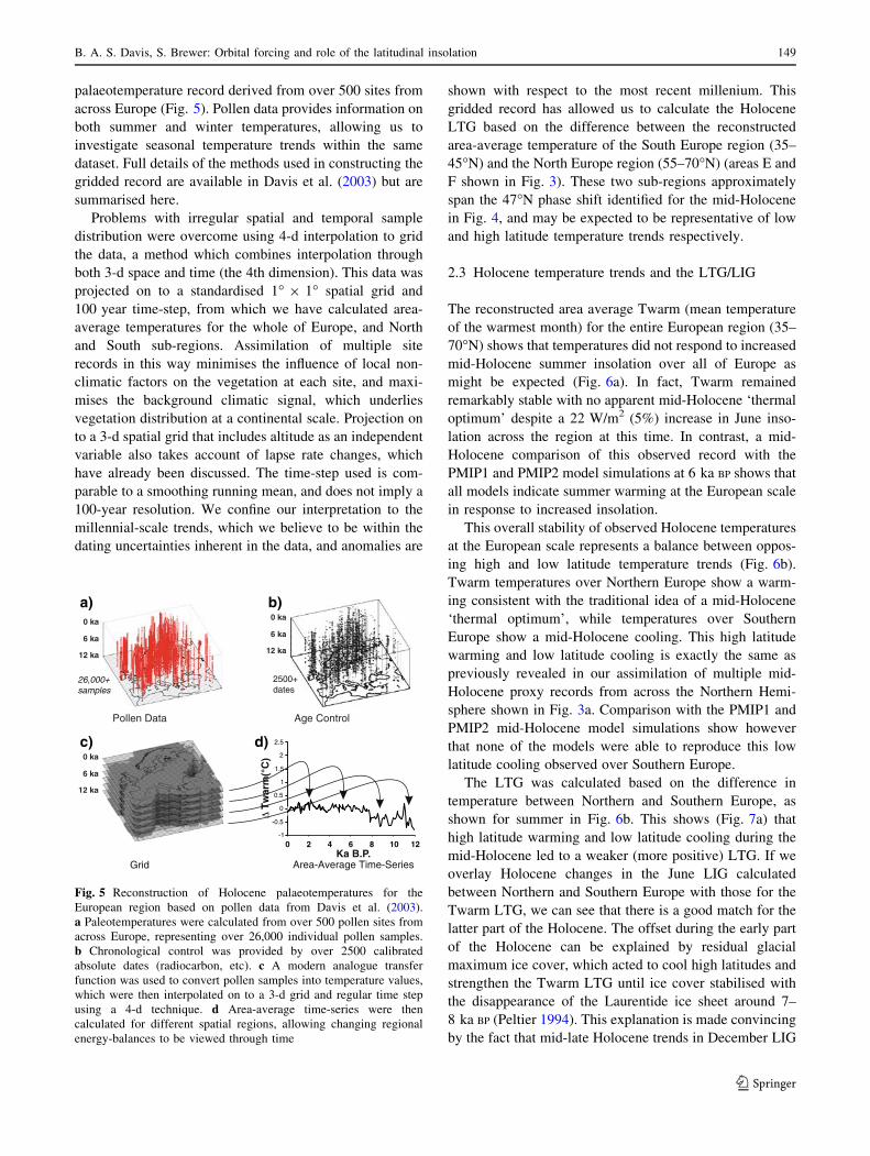
palaeotemperature record derived from over 500 sites from

across Europe (Fig. 5). Pollen data provides information on

both summer and winter temperatures, allowing us to

investigate seasonal temperature trends within the same

dataset. Full details of the methods used in constructing the

gridded record are available in Davis et al. (2003) but are

summarised here.

Problems with irregular spatial and temporal sample

distribution were overcome using 4-d interpolation to grid

the data, a method which combines interpolation through

both 3-d space and time (the 4th dimension). This data was

projected on to a standardised 1� 9 1� spatial grid and

100 year time-step, from which we have calculated area-

average temperatures for the whole of Europe, and North

and South sub-regions. Assimilation of multiple site

records in this way minimises the influence of local non-

climatic factors on the vegetation at each site, and maxi-

mises the background climatic signal, which underlies

vegetation distribution at a continental scale. Projection on

to a 3-d spatial grid that includes altitude as an independent

variable also takes account of lapse rate changes, which

have already been discussed. The time-step used is com-

parable to a smoothing running mean, and does not imply a

100-year resolution. We confine our interpretation to the

millennial-scale trends, which we believe to be within the

dating uncertainties inherent in the data, and anomalies are

shown with respect to the most recent millenium. This

gridded record has allowed us to calculate the Holocene

LTG based on the difference between the reconstructed

area-average temperature of the South Europe region (35–

45�N) and the North Europe region (55–70�N) (areas E and

F shown in Fig. 3). These two sub-regions approximately

span the 47�N phase shift identified for the mid-Holocene

in Fig. 4, and may be expected to be representative of low

and high latitude temperature trends respectively.

2.3 Holocene temperature trends and the LTG/LIG

The reconstructed area average Twarm (mean temperature

of the warmest month) for the entire European region (35–

70�N) shows that temperatures did not respond to increased

mid-Holocene summer insolation over all of Europe as

might be expected (Fig. 6a). In fact, Twarm remained

remarkably stable with no apparent mid-Holocene ‘thermal

optimum’ despite a 22 W/m2 (5%) increase in June inso-

lation across the region at this time. In contrast, a mid-

Holocene comparison of this observed record with the

PMIP1 and PMIP2 model simulations at 6 ka BP shows that

all models indicate summer warming at the European scale

in response to increased insolation.

This overall stability of observed Holocene temperatures

at the European scale represents a balance between oppos-

ing high and low latitude temperature trends (Fig. 6b).

Twarm temperatures over Northern Europe show a warm-

ing consistent with the traditional idea of a mid-Holocene

‘thermal optimum’, while temperatures over Southern

Europe show a mid-Holocene cooling. This high latitude

warming and low latitude cooling is exactly the same as

previously revealed in our assimilation of multiple mid-

Holocene proxy records from across the Northern Hemi-

sphere shown in Fig. 3a. Comparison with the PMIP1 and

PMIP2 mid-Holocene model simulations show however

that none of the models were able to reproduce this low

latitude cooling observed over Southern Europe.

The LTG was calculated based on the difference in

temperature between Northern and Southern Europe, as

shown for summer in Fig. 6b. This shows (Fig. 7a) that

high latitude warming and low latitude cooling during the

mid-Holocene led to a weaker (more positive) LTG. If we

overlay Holocene changes in the June LIG calculated

between Northern and Southern Europe with those for the

Twarm LTG, we can see that there is a good match for the

latter part of the Holocene. The offset during the early part

of the Holocene can be explained by residual glacial

maximum ice cover, which acted to cool high latitudes and

strengthen the Twarm LTG until ice cover stabilised with

the disappearance of the Laurentide ice sheet around 7–

8 ka BP (Peltier 1994). This explanation is made convincing

by the fact that mid-late Holocene trends in December LIG

0 ka

6 ka

12 ka

Pollen Data

Grid

Age Control

0 ka

6 ka

12 ka

0 ka

6 ka

12 ka

-1

-0.5

0

0.5

1

1.5

2

2.5

1086420 12Ka B.P.

∆ T

war

m(°

C)

Area-Average Time-Series

26,000+samples

2500+dates

a) b)

d)c)

Fig. 5 Reconstruction of Holocene palaeotemperatures for the

European region based on pollen data from Davis et al. (2003).

a Paleotemperatures were calculated from over 500 pollen sites from

across Europe, representing over 26,000 individual pollen samples.

b Chronological control was provided by over 2500 calibrated

absolute dates (radiocarbon, etc). c A modern analogue transfer

function was used to convert pollen samples into temperature values,

which were then interpolated on to a 3-d grid and regular time step

using a 4-d technique. d Area-average time-series were then

calculated for different spatial regions, allowing changing regional

energy-balances to be viewed through time


123

and Tcold (mean temperature of the coldest month) LTG

also match (Fig. 7b), whilst at the same time being very

different from those of their summer counterparts. Again,

the effect of ice cover is shown to dominate the Tcold LTG

during the early part of the Holocene. Figure 7a also shows

the significance of the data-model mismatch highlighted in

Fig. 6b, where the lack of low latitude summer cooling in

the PMIP1 and PMIP2 model simulations causes models to

underestimate the weakening of the summer LTG observed

in the mid-Holocene. The same model simulations for the

winter LTG are shown in Fig. 7b, but these are within the

error bounds of the reconstruction.

2.4 The Holocene LTG and Northern Hemisphere

climate

These results demonstrate systematic changes in the LTG

across Europe, but do these also reflect changes in the

global climate system? The LTG controls the latitudinal

location of the main climate zones, including the Hadley

Cell, and with it the ITCZ and Monsoon system (Flohn

1965) (Fig. 8a inset). We would therefore expect these

systems to show a comparable response to the recon-

structed LTG during the Holocene. The nature of this

relationship is demonstrated every year as these systems

migrate northwards in summer when the LTG is weak, and

southward in winter when the LTG is strong. Compilations

of lake level reconstructions from across North Africa

indicate that water levels were highest between 10 and

6 ka, associated with a northward extension of the African

Monsoon system (Jolly et al. 1998; Damnati 2000). This

same period is also recorded by rapid speleothem deposi-

tion in Oman, suggesting a concurrent expansion of the

Indian Monsoon (Fleitmann et al. 2003b). Figure 8a shows

the timing of this mega-Monsoon together with a more

continuous isotopic record of the Indian Monsoon from the

Oman site (Fleitmann et al. 2003a), and a record of ITCZ

position recorded in marine sediments in the southern

Caribbean (Haug et al. 2001). All these observations sug-

gest a northward expansion of the Hadley Cell during the

-1

-0.5

0

0.5

1

1.5

2

2.5

0 2 4 6 8 10 12-20

-10

0

10

20

30

40

50

Ka B.P.

-2

-1.5

-1

-0.5

0

0.5

1

1.5

2

2.5

0 2 4 6 8 10 12

Ka B.P.

-1

-0.5

0

0.5

1

1.5

2

2.5

0 2 4 6 8 10 12-20

-10

0

10

20

30

40

50

Summer Temperature:Europe

∆Tw

arm

K()

∆Tw

arm

K()

6ka Models

∆Ju

ne

Inso

lati

on

(w

/m)2

South

NorthEurope

Europe

Summer Temperature:North & South Europe

NorthEurope

SouthEurope

Europe

Summer

Summer

A AO AOV

A AO AOV

6ka Models

Insolation

a)

b)

Fig. 6 Reconstructed warmest month (summer) temperatures

(Twarm) for Europe during the Holocene compared with PMIP1

and PMIP2 mid-Holocene (6 ka) climate model simulations. Ensem-

ble results are shown for 16 Atmosphere-only (A), and 9 fully coupled

Atmosphere–Ocean (AO) and 3 Atmosphere–Ocean–Vegetation

(AOV) models, with errors calculated as 1 SD of the inter-model

variance. Errors are also shown for the observed temperature at 6 ka aThe mean summer temperature of Europe shows no mid-Holocene

thermal optimum in response to increased summer insolation (shown

here by mean mid-month June insolation over the region from Berger

1978). In contrast, PMIP model simulations all show warming. b The

stability of Holocene summer temperatures at the European scale

represents a balance between warming over North Europe and cooling

over South Europe. The low latitude cooling observed over South

Europe is not reproduced in the PMIP model simulations, which all

indicate low latitude warming at 6 ka


123

Holocene consistent with our reconstruction of a weaken-

ing mid-Holocene Twarm LTG. Climate models however

reproduce little change in LTG between the present day

and the mid-Holocene (Fig. 7a), a factor that may explain

why models continue to have difficulty reproducing the

northward shift of the African Monsoon into the sub-Tro-

pics (Joussaume et al. 1999; Braconnot et al. 2000; Valdes

2003; Braconnot et al. 2004; Braconnot et al. 2007a). One

answer to this problem has been to incorporate vegetation

feedbacks in AOV-GCM’s, which more accurately repre-

sent these land surface changes at this time (Ganopolski

et al. 1998). The change from desert to savannah lowers

albedo and increases surface warming compared to AO-

GCM’s (as shown in Fig. 9), which helps drive convection

and land–ocean temperature contrast which also boost

Monsoon strength. However, the observational evidence of

cooler land surface conditions may indicate that this kind

of feedback is unrealistic. Similarly, evidence of cooler

mid-Holocene SST’s in the sub-tropical North Atlantic,

although far from conclusive, would also contradict model

mechanisms for enhancing the West African Monsoon

based on warmer summer SST’s in this region (Kutzbach

and Liu 1997; Braconnot et al. 2007b). Zhao et al. (2005)

have highlighted the difficulty in evaluating this mecha-

nism, which appears to rely on a short late summer warming

of SST’s that may be difficult to detect in the palaeo SST

record. However, irrespective of these problems, this model

mechanism still fails to explain the northward extent of the

African Monsoon, while appearing to cause a contradictory

decrease in the strength of the Indian Monsoon (Braconnot

et al. 2007b).

Evidence of extensive low latitude cooling also offers an

alternative perspective for interpreting the proxy evidence

of Monsoon expansion. Climate modelling experiments

have focussed almost exclusively on increasing precipita-

tion to resolve data-model discrepancies (Joussaume

et al. 1999, Braconnot et al. 2007a), despite the fact that

most proxies reflect positive changes in P–E that are

also influenced by temperature. In this way, cooling as

well as increased precipitation could equally explain

the favourable shift in the moisture balance reflected in

vegetation and lake-level proxies that indicate Monsoon

enlargement.

Whilst the Monsoon and ITCZ are prominent summer

climate modes, winter in the Northern Hemisphere is

strongly influenced by the AO extra-tropical atmospheric

circulation mode. The AO also includes the North Atlantic

Oscillation (NAO), which we refer to herein as a regional

expression of the AO. A major part of recent high latitude

warming has been attributed to a shift to a more positive

winter AO (Moritz et al. 2002). This change in mid-latitude

westerly circulation leads to warm air advection over

Northern Europe, which experiences mild wet winters,

while Southern Europe experiences cool dry winters

(Visbeck 2002). This higher latitude warming and lower

latitude cooling leads to a weakening of the LTG across

0 2 4 6 8 10 12Ka B.P.

-3

2

1

0

-1

-2

∆D

ecem

ber

LIG

(w

/)

m2

-20

-10

0

10

20

∆T c

old

LTG

(K

)

∆N

H Ic

e C

ove

r(%

)

50

100

150

200

250

0

South

NorthEurope LTG

Winter LatitudinalTemperature Gradient( )North - South Europe

LTG

IceLIG

Winter-30

-20 2 4 6 8 10 12

-6

Ka B.P.

Summer LatitudinalTemperature Gradient(North - South Europe)

3

2

1

0

-1

9

6

3

0

-3

50

100

150

200

250

∆Ju

ne

LIG

(w

/m)2

∆Tw

arm

KLT

G (

)

0

∆N

H Ic

e C

ove

r(%

)

South

NorthEurope LTG

LTG

IceLIG

Summer

A AO AOV

AO AOVA

6ka Models

6ka Models

a)

b)

Fig. 7 Changes in seasonal

reconstructed Holocene LTG

can be explained by seasonal

changes in LIG (mid-month

values from Berger 1978), and

Northern Hemisphere ice cover

(from Peltier 1994).

Temperature and insolation

gradients were calculated by

deducting mean anomaly values

for Northern Europe from those

of Southern Europe. a Summer

(Twarm) LTG compared with

the June LIG and ice cover. The

LTG is also compared here with

PMIP mid-Holocene climate

model simulations, which all

underestimate LTG weakening

due to the lack of low latitude

cooling shown in Fig. 6b.

b Winter (Tcold) LTG

compared with the December

LIG and ice cover. PMIP mid-

Holocene model simulations are

also shown and compare more

favourably with the observed

LTG than in summer


123

0 2 4 6 8 10 12Ka BP

40

60

80

100 % N

. pac

hy. (

s.)

-3

1

0

-1

-2

∆T

cold

KLT

G (

)

+

-

ArcticOscillation

% M

ild/W

et W

inte

r

200

100

0

-10

0

10

20

2

-1

1

-1

0

0

ITCZFurtherNorth

IncreasedMonsoonPrecipitation

Cariaco Basin

Oman

∆Tw

arm

KLT

G (

)

∆T i

tan

ium

(%)

∆δO

18

0 2 4 6 8 10 12Ka BP

Mega-Monsoon

Norwegian Mnts

Norwegian Sea

8

4

0

-4

-4 -2 0 2 4Winter AO Index

Tco

ld L

TG

(C

)∆

° 20th Century

-10-5

05

1015

30N 35N 40N 45N

Annual

LTG

()

∆K

Latitude of Sub-Tropical High

WeakerLTG

atitudinalemperatureradient

(Summer)

Inset: Shows monthly position of Sub-Tropical Highpressure against LTG. Weak LTG in summer resultsin maximum poleward position.

Inset: Shows relationship between winter LTG acrossEurope and AO during the 20th Century. Strong +AOresults in weak LTG (r =0.56)2

WeakerLTG


(Winter)

WarmerSST's

Wetter/MilderWinters

SummerITCZ/Monsoon

ITCZMonsoon

Warm

Current

AO

WinterArctic Oscillation

South

NorthEurope

South

NorthEurope

1 2

4 3

1

2

Sub-TropicalHigh Pressure

North

South

3

4

LTGLTG

LTG

LTG

Atlantic Waters in Barents SeaAtlantic Waters in Barents SeaAtlantic Waters in Barents Sea

-8

a)

b)

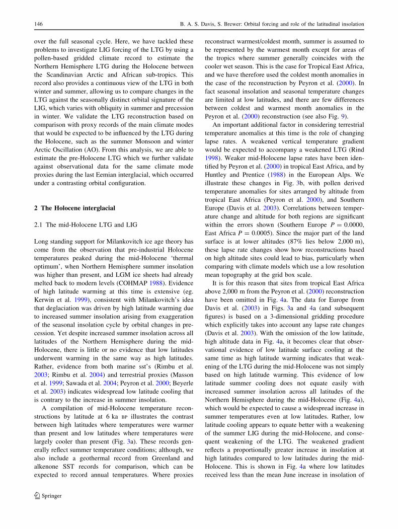
Fig. 8 A comparison of the seasonal LTG reconstructions from

Fig. 7 with palaeoclimate records of the main Northern Hemisphere

climate modes during the Holocene. a Weakening of the summer

LTG during the mid-Holocene suggests a poleward displacement of

the sub-tropical high pressure and Hadley Cell (Flohn 1965; see

inset). This is supported by � poleward displacement of the ITCZ

recorded by Titanium in sediments at Cariaco Basin, Venezuela

(Haug et al. 2001), as well as ` increased Monsoon intensity

recorded in the isotopic composition of a speleothem at Hoti Cave,

Oman (Fleitmann et al. 2003a). The black bar indicates high rates of

speleothem accumulation associated with the most intense Monsoon

period (Fleitmann et al. 2003b). d Weakening of the winter LTG

during the mid-Holocene would suggest a more positive AO.

Positive AO-type circulation results in warm air advection into

North Europe and other high latitudes (Moritz et al. 2002), and cool

air advection into South Europe (Visbeck 2002) resulting in a

weakened LTG. Comparison of the twentieth century winter LTG

over Europe derived from instrumental data (Mitchell et al. 2002)

and the AO index (Thompson and Wallace 1999) show a strong

relationship (see inset). The correlation value is based on the mean

DJF index and the Tcold (coldest month) temperature gradient

(1901–2000 AD). This is supported for the Holocene by ´ an

independent reconstruction of AO (NAO) based on glacier mass-

balance in Norway (Nesje et al. 2000, 2001), as well as ˆ a

foraminifera record from sediment core HM52-43 in the Norwegian

Sea (Fronval and Jansen 1996). The decline of polar N. pachyderma(s.) in the mid-Holocene (note inverted scale) is interpreted as the

result of increased northward penetration of warm Atlantic waters

into the Norwegian Sea, a period that also coincides with the

maximum penetration of Atlantic waters recorded in the Barents Sea

(Duplessy et al. 2001) shown by the black bar. It has been shown

the northward extent of warm Atlantic waters in this region is

strongly related to wind stress arising from a positive AO (NAO)

(Blindheim et al. 2000)


123

Europe that is reflected in a close correlation between the

Tcold LTG, and the AO during the twentieth Century

(r2 = 0.56) (Fig. 8b inset). We reconstruct a mid-Holocene

weakening of the Tcold LTG that suggests this period was

associated with a strong positive AO-type circulation. This

inference is supported by the similarity between our tem-

perature based reconstruction, and an independent

reconstruction of Holocene NAO (AO) from glacier mass

balance in Norway (Nesje et al. 2000; Nesje et al. 2001).

Changes in the AO also influence wind stress across

the North Atlantic, helping to drive warm Atlantic waters

northward along the Norwegian Current during positive

NAO (AO) conditions (Blindheim et al. 2000). Evidence

from this region that the maximum extension of warm

Atlantic waters occurred in the early mid-Holocene

(Fronval and Jansen 1996; Duplessy et al. 2001) is there-

fore consistent with these Holocene AO (NAO)

reconstructions (Fig. 8b). The change in LTG in winter is

smaller than in summer, and climate model simulations are

within the error-bars of the reconstruction (Fig. 7b), but

model response may be expected to be closer to the

observed because in winter the LIG and direct radiative

forcing arise from the same insolation changes (Fig. 9).

Models also appear to respond to different forcing mech-

anisms to that observed, with AO-GCM models showing

little change in the NAO at this time (Gladstone et al.

2006). The weaker winter LTG shown in the AOV-GCM

models appears to be the result of unrealistic high lati-

tude winter warming, at least over Northern Europe

(Fig. 9). This is attributed to local feedbacks such as

reduced sea-ice (Ganopolski et al. 1998; Claussen 2003;

Gallimore et al. 2005), and not advection processes such as

the NAO.

Overall, comparison of our Holocene LTG reconstruc-

tion with a mid-Holocene multi-proxy data compilation

(Fig. 3a), and records of summer Monsoon/ITCZ and

winter AO climate modes (Fig. 8a, b) demonstrate that this

record is representative of the Northern Hemisphere LTG.

Differences in LTG trends between winter and summer

also closely match trends in the LIG, consistent with LIG

forcing of the LTG. Differences between the LTG and LIG

in the early Holocene can be attributed to additional

cooling of high latitude temperatures by residual LGM

ice sheets. Following from these observations of LIG

and Ice Sheet forcing of Holocene climate, further vali-

dation was undertaken through comparison of LIG and Ice

Sheet forcing with climate during the earlier Eemian

interglacial.

3 The Eemian interglacial

A major challenge to Milankovitch theory has come from

evidence that deglaciation in the lead-up to the last inter-

glacial (Eemian/OIS-5e) began before changes in

precession had led to any significant increase in high lati-

tude summer insolation (Gallup et al. 2002). Changes in

obliquity and precession occurred together during the

Holocene, but obliquity led precession into the Eemian,

providing a test of our orbital forcing theory. Observed

climate change during the Eemian was also very different

than the Holocene, with Milankovitch theory providing

little explanation as to why Eemian interglacial conditions

lasted twice as long in Southern Europe as Northern Eur-

ope (Kukla 2000), or why summer and winter temperatures

peaked at different times (Zagwijn 1996).

∆Te

mp

erat

ure

°(C

)

-12

-10

-8

-6

-4

-2

0

2

4

6

-20 -10 0 10 20

Latitude (North)

30 40 50 60 70 80 90

∆Te

mp

erat

ure

°(C

)

-12

-10

-8

-6

-4

-2

0

2

4

6

-20 -10 0 10 20

Latitude (North)

30 40 50 60 70 80 90

-20

-10

10

30

-30

0

20

∆D

ecem

ber

Inso

lati

on

w/m

2(

)

WinterSummer

Observed (±1sd)

A

∆Ju

ne

Inso

lati

on

w/m

2(

)

10

30

0

20

-20

-10

-30

8

10

8

10

-40 -40

A

AOV-GCM Ensemble (±1sd)

Observed (±1sd)

AOV-GCM Ensemble (±1sd)

a) b)

verage ofall sites'D'

verage ofall sites'D'

Fig. 9 A summer and winter mid-Holocene comparison of climate

model and observed latitudinal temperature anomalies in the Afro-

European sector (10 W–50�E), together with respective June and

December insolation forcing. Analysis shows the ensemble response

of 3 Atmosphere–Ocean–Vegetation (AOV) model simulations.

Seasonal pollen-climate reconstructions are shown based on latitudi-

nal average temperatures from north to south Europe, together with an

average of individual sites in Tropical East Africa from Peyron et al.

2000(as shown for summer in Figs. 3 and 4a). Models over estimate

low latitude warming in summer and high latitude warming in winter


123

3.1 Estimating the Eemian LTG

Our initial Holocene based investigations indicated that the

LTG is a function of the LIG and ice cover. We were

therefore able to estimate the Eemian LTG using astro-

nomical calculations to determine the LIG (Berger 1978),

while ice cover was estimated using a marine isotope derived

sea level reconstruction whose chronology was based on the

U–Th dated coral record for Termination II (Waelbroeck

et al. 2002). We converted sea level to Northern Hemisphere

ice cover according to the Termination I deglaciation

sequence (Peltier 1994) (Appendix 2). We therefore assume

that the contribution to sea level by melting Northern

Hemisphere ice during Termination II was the same as

Termination I, as was the relationship between ice volume

and surface area. Evidence indicates that higher sea levels

were experienced during the Eemian than the Holocene as a

result of a reduced Greenland Ice sheet. For this period, we

have scaled the Eemian sea level maximum from the sea

level reconstruction (?6.3 m) against a ‘best estimate’ of a

maximum 67% reduction in the Greenland Ice sheet (Cuffey

and Marshall 2000). A multiple linear regression was then

used to calibrate ice cover and June/December LIG against

the Twarm LTG (r2 = 0.82) and Tcold LTG (r2 = 0.89)

respectively, based on the Holocene calibration period. The

relative relationship between the different forcings and

estimated/observed LTG is shown in Fig. 10. This shows

that a weakening LTG (more positive) generally leads

decreasing ice cover, while a strengthening LTG (more

negative) leads increasing ice cover, suggesting that ice

cover is being forced by the LIG through its influence on the

LTG. Estimated LTG values for cold glacial periods may

however be underestimated due to decreases in water vapour

content and therefore the poleward flux of latent and sensible

heat (Pierrehumbert 2002), although values of 9–10 K dur-

ing the LGM appear comparable with estimates of 16–17 K

from the Greenland deuterium ice core record located at

72 N (Masson-Delmotte et al. 2005).

Tcold LTG (estimated)

Ice

∆N

H Ic

e C

ove

r(%

)

Ka B.P.

-100

100

300

500

700

110 115 120 125 130 135 140 145 150 1550 5 10 15 20 25 30

4

2

0

-2

-4

-6

-8

-10

-12MIS 5d MIS 5e MIS 6MIS 1 MIS 2

Modern

Ka B.P.

40

20

0

-20

-40

Tcold LTG estimated from Ice Cover and December LIG forcing

∆K

LTG

()

December LIG

∆D

ecem

ber

LIG

(w

/)

m2

Twarm LTG estimated from Ice Cover and June LIG forcing∆

NH

Ice

Co

ver

(%)

Ka B.P.

-100

100

300

500

700

900

110 115 120 125 130 135 140 145 150 1550 5 10 15 20 25 30

4

2

0

-2

-4

-6

-8

-10

-12MIS 5d MIS 5e MIS 6MIS 1 MIS 2

Modern

Ka B.P.

20

10

0

-10

-20

Twarm LTG (estimated)June LIG

Ice

∆K

LTG

()

∆Ju

ne

LIG

(w

/m)2

Calibration Period

Calibration Period

Twarm LTG (observed)

Tcold LTG (observed)

Holocene Eemian

Holocene Eemian

Fig. 10 Estimates of pre-Holocene summer and winter LTG were

made using ice cover and LIG forcings demonstrated in Fig. 7.

Calibration was undertaken over the Holocene using the observed

LTG. Northern Hemisphere ice cover was calculated back to the

LGM based on Peltier (1994), and thereafter estimated from the sea

level reconstruction of Waelbroeck et al. (2002). Ice cover estimation

is based on the relationship between sea level and Northern

Hemisphere ice cover observed over the Termination I period, and

therefore assumes a similar configuration of ice cover and contribu-

tion to sea level over the Termination II deglaciation period. The

Termination II mid-point is taken to be 135 Ka BP, in agreement with

coral evidence (Waelbroeck et al. 2002). Evidence also indicates that

higher sea levels were experienced during the Eemian than the

Holocene as a result of a reduced Greenland Ice sheet. For this period,

we have scaled the Eemian sea level maximum from the sea level

reconstruction (?6.3 m) against a ‘best estimate’ of a maximum 67%

reduction in the Greenland Ice sheet (Cuffey and Marshall 2000).

June and December LIG were derived from astronomical calculations

(Berger 1978). A simple multiple linear regression was then used to

calibrate ice cover and June/December LIG against Twarm LTG

(r2 = 0.82) and Tcold LTG (r2 = 0.89) respectively, based on the

Holocene calibration period


123

3.2 The Eemian LTG and Northern Hemisphere

climate

Changes in our empirically estimated Eemian LTG

(explained in Sect. 3.1) follow a different pattern from that

of the Holocene, resulting in an off-set in the timing of

winter and summer LTG weakening (Fig. 11b) that reflects

the off-set in precession and obliquity changes (Fig. 11a).

The early change in obliquity meant that the LTG weakened

earlier in summer than in winter during Termination II. This

would explain the earlier onset of high latitude summer

warming and deglaciation indicated by the independently

dated coral-based sea level evidence. Evidence of early

Eemian warmth over Northern Europe is provided by the

onset of rapid growth in radiometrically dated speleothems.

These indicate the start of interglacial conditions at around

132 ± 5.0 ka BP in Norway (Lauritzen 1995), 133 ± 2.4 ka

BP in England (Baker et al. 1995) and 135 ± 1.2 ka BP at

40

60

80

100

% N

. pac

hy. (

s.)

Ka B.P.

0

-2

2

-4

110 115 120 125 130 135 1401050 5 10 15 20

∆LT

G (

K)

4

2

0

-2

-4

-6

-8

∆T

(K)

Ka B.P.

2

0

-2

-4

% N

. pac

hy. (

s.)

100

-4

60

80

0

-2

2

∆T

(K)

Mega-Monsoon

Mega-Monsoon

NetherlandsTemperature

NetherlandsTemperature

Duration ofHolocene Interglacial

Duration ofEemian Interglacial

∆LT

G (

K)

Ice

LTGWinter

T(Summer)

warmTWinter)

cold(

LTGSummer

Ice

a)

b)

c)

d)

e)

f)

15515014525 30

MIS1 MIS2 MIS 5d MIS 5e MIS 6

16

17

12

13

14

15

Marine Isotope Stage

16

17

13

14

15

CaliforniaCurrentWarmer

SSTNorwegianSea

Warmer SST( )+AO

CaliforniaCurrentWarmer

SSTNorwegian

SeaWarmer SST

( )+AO

Alk

eno

ne

SS

T (

K)

Alk

eno

ne

SS

T (

K)

g)

ITCZMonsoon

2

South

North

Europe

Warm

Current

AO

4

6

Ice

LIGSummer& Winter

For

cing

LTG

Mon

soon

Arc

ticO

scill

atio

nTe

mpe

ratu

re

LTG


Sub

-Tro

pica

lO

cean

Gyr

e

South

North

Europe

Inte

rgla

cial

Dur

atio

n

5

110 115 120 125 135 140105 1551501450 5 10 15 20 25 30

Holocene Eemian

TWinter)

cold(

T(Summer)

warm

North Europe

South Europe

North Europe

South Europe

LTG in Summerweakens earlierthan in Winter

LTG in Summerweakens at similartime as Winter

Obliquity changesat similar time asprecession

-20

0

20

40

-8

0

8

16Obliquity changesearlier thanprecession

LIGSummer(Obliquity)

LIGWinter

(Precession)60N

10N

60N

10N

∆Ju

ne

Inso

lati

on

(w/m

)2

∆L

IG(w

/m)2

-10

60NSummer

10NSummer

Summer & Winterchange together

Summer changesearlier than Winter

Fig. 11 LIG forcing of the LTG explains differences in winter (grey)

and summer (black) climate between Holocene and Eemian intergla-

cials (vertical arrows), which occurred under different orbital

configurations. a Precession and obliquity were in phase during the

Holocene, but out of phase during the Eemian (Berger 1978),

resulting in similar differences in the phasing of the LIG between

winter (December) and summer (June). Summer (June) insolation is

shown for 60�N (dashed line) and 10�N (dashed dotted line) for

comparison. Northern Hemisphere ice cover is from Fig. 9 (dottedblack line). b Different phasing of precession and obliquity is

reflected in the estimated LTG (from Fig. 10), which weakens earlier

in summer than winter during the Eemian. c Early weakening of the

summer LTG during the onset of the Eemian is supported by evidence

of early warming of the California current (Herbert et al. 2001), which

would have been influenced by the subsequent poleward shift in the

sub-tropical high pressure and related ocean gyre. d This would also

explain the early onset of ‘Mega-Monsoon’ conditions during the

Eemian, as indicated by high rates of speleothem deposition at Hoti

Cave in Oman, and dated by U–Th analysis (Fleitmann et al. 2003b).

e The penetration of warm Atlantic waters into the Norwegian Sea

recorded in two marine cores during the Holocene (HM52-43) and

Eemian (ODP 644) by a decline in N.pachy.(s) (data and chronology

from Fronval and Jansen 1996). This is interpreted as a result of a

positive winter AO (see text and Fig. 8b), which was in-phase with

the mega-Monsoon period during the Holocene but delayed during the

Eemian. f Netherlands winter and summer temperatures peaked

around the same time during the Holocene but summers temperatures

peaked before winter temperatures during the Eemian, consistent with

earlier weakening of the summer LTG. The Holocene reconstruction

is pollen based (see text, Appendix 2) while the Eemian reconstruc-

tion is macrofossil based (Zagwijn 1996). Eemian chronology is

based on the original authors local sea level curve adjusted to the

Waelbroeck et al. (2002) reference sea level curve. g The duration of

the Holocene and Eemian Interglacial over North and South Europe

(taken from Kukla 2000) shows significant differences that indicates a

strong LTG in the later Eemian, in agreement with (b). The

chronology is taken from the author’s original timescale, although

the dashed extension to North Europe during the Eemian reflects the

earlier warming suggested by the reference sea level curve used here

and as shown in (f)


123

altitude in the Austrian Alps (Spotl et al. 2002). This evi-

dence supports an early start to the Eemian climatic

amelioration, while seasonal temperature reconstructions

from the Netherlands (Zagwijn 1996) and elsewhere in

Europe (Aalbersberg and Litt 1998; Rousseau et al. 2006)

suggest that this warming was characterised primarily by

increases in summer temperatures, while winter tempera-

tures peaked later in the Eemian. This is different from the

Holocene when summer and winter temperatures peaked at

around the same time in the mid-Holocene in Northern

Europe, illustrated by a pollen based temperature recon-

struction for the Netherlands in Fig. 11f.

Early weakening of the summer LTG may also be

reflected in low latitude records of Monsoon expansion,

with U–Th dated evidence from Oman (Fleitmann et al.

2003b) indicating that Mega-Monsoon conditions became

established as early as 135 Ka B.P (Fig. 11d). This pre-

dates any significant precession-driven increase in summer

insolation and therefore any direct radiative forcing of the

Monsoon system, but is entirely consistent with our pro-

posed dynamic forcing of the Monsoon arising from a

weakened summer LTG. The same early weakening of the

summer LTG would also be expected to cause a northward

shift in the sub-tropical high pressure and associated ocean

gyres. This may therefore provide an explanation for early

warming of the California current (Fig. 11c), which has

been suggested as the main influence on the Devils Hole

speleothem record (Herbert et al. 2001). The well dated

record at Devils Hole has been cited as an important

criticism of Milankovitch theory, since it suggests inter-

glacial conditions began as early as 142 ± 3.0 Ka, well

before any increase in high latitude summer insolation

(Winograd et al. 1992; Broecker 1992; Winograd et al.

2002).

Observational evidence indicates that the latter part of

Eemian MIS5e was associated with a peak in winter

warming over Northern Europe associated with a wetter

and more oceanic climate (Zagwijn 1996, Aalbersberg and

Litt 1998). It has been suggested this oceanic climate was

the result of a persistent positive AO (NAO) type circula-

tion (Felis et al. 2004). This is in agreement with our

evidence for maximum weakening of the winter LTG at

this time, which also exceeds that experienced during the

Holocene. The timing of this weakening and our inference

that it reflects development of a strong AO-type circulation

is entirely in agreement with the observed expansion of

warm Atlantic waters into the Norwegian Sea at this time

(Fronval and Jansen 1996) (Fig. 11e).

A significant source of debate about the Eemian has

centred on the length of the interglacial itself. Estimates

from Northern Europe indicate that interglacial conditions

may not have extended much longer than the current

Holocene, while evidence from Southern Europe indicate

that warm climate conditions persisted almost twice as long

again (Fig. 11 g) (Kukla 2000). This would suggest that

LTG’s were particularly strong in the closing stages of the

Eemian (OIS-5d) as the North cooled but the South

remained warm (Tzedakis 2003). Again, our model results

fully support this observational evidence, indicating strong

LTG’s due to strong LIG’s at this time (Fig. 11b). This

resulted in temperature gradients across Europe that were

stronger than today even when Eemian ice cover (Fig. 11a)

was similar to today’s levels.

4 Discussion

Glacial-interglacial cycles represent the largest changes in

the Earth’s climate in its recent history, yet these climatic

fluctuations have occurred without any major variation in

total global insolation received from the Sun. Rather, the

dominant forcing has been seasonal and latitudinal varia-

tions in insolation arising from orbital changes in

precession and obliquity. Understanding the climate system

response to these insolation changes requires both a sea-

sonal and latitudinal perspective, but this has generally

been limited by a lack of records from low latitudes and

proxies sensitive to the winter season. When viewed from

both low as well as high latitudes and throughout both

winter and summer seasons, the climate system response to

insolation appears to be more strongly dependant on lati-

tude than season. This suggests that summer warming of

high latitudes during interglacials occurred not so much

because of an increase in summer insolation, but because

the increase in summer insolation was greater over high

latitudes than low latitudes. This polar-amplification is not

generally shown in climate models, which appear to over-

emphasise the seasonal rather than this latitudinal response

to insolation. This suggests models underestimate the role

of the LIG in driving polar amplification of global mean

temperature through the LTG, and therefore may overes-

timate the role of Greenhouse gases in driving high latitude

warming through global mean temperature over orbital

timescales (Luthi et al. 2008). The sensitivity of the LTG to

LIG forcing also places greater emphasis on obliquity in

summer and precession in winter in driving high latitude

warming, rather than high latitude summer insolation

changes, which are mainly driven by precession. This

could help explain the apparent paradox of synchronous

glacial–interglacial cycles between hemispheres with

opposing precession-driven summer insolation receipts,

because obliquity-driven summer LIG changes are in-phase

between hemispheres (Fig. 12). Furthermore, many aspects

of the Earth’s climate are influenced by the LTG, and

the sensitivity of the LTG to LIG changes could help

explain the propagation of these obliquity and precession


123

signatures throughout the climate system. In particular, this

could explain the presence of obliquity signals in climate

records at low latitudes where insolation changes are

otherwise dominated by precession. In the same way, the

LTG is also influenced by high latitude ice cover, which

provides a way in which ice cover changes can also be

overprinted on climate records from lower latitudes. The

sensitivity shown by the LTG to LIG and ice cover forcing

may therefore offer an alternative perspective not just on

orbital forcing of high latitude warming, but also on orbital

forcing of low latitude climate.

4.1 Monsoons

The Monsoon system is probably second only to the polar

ice sheets in global climatic importance, and the develop-

ment of mega-Monsoons are the largest climatic changes

associated with non-glacial climates. As with high latitude

ice sheets it is precession driven changes in summer

insolation that are considered to underlie long-term orbital

forcing of the Monsoon system (Rossignol-Strick et al.

1982; Kutzbach and Street-Perrott 1985). Records of

Monsoon climate variability show a clear precession sig-

nal, with a contrary inter-hemispheric response that

would be expected from precession forcing (Ruddiman

2006). Yet such records also include a strong obliquity

signal (Clemens and Prell 2007), particularly prior to

1 million year BP when Northern Hemisphere ice sheets

were poorly developed (deMenocal 1995; Lourens et al.

1996, 2001, Larrasoana et al. 2003). This obliquity signal is

difficult to explain based on simple summer insolation

forcing of the Monsoon system alone. However, this

response is consistent with LTG forcing of the Monsoon as

a result of obliquity driven changes in the summer LIG that

we identify here, particularly when the influence of ice

cover on the LTG prior to 1 million year BP would have

been limited. Similarly, the occurrence of major Monsoon

periods at times when precessional forcing was relatively

weak (Rossignol-Strick et al. 1998), but obliquity still

strong, may also be explained by this mechanism.

Inso

latio

nG

radi

ent

(w/m

∆Ju

ne )2

∆D

ecem

ber

)

Inso

latio

nG

radi

ent

(w/m

2

0 100 200

0 100 200

∆D

ecem

ber

)

Inso

latio

nG

radi

ent

(w/m

2

In Phase

Inso

latio

nG

radi

ent

(w/m

∆Ju

ne )2

Counter Phase

Ka BP

Ka BP

NorthernHemisphere

SouthernHemisphere

NorthernHemisphere

SouthernHemisphere

Inso

latio

n(w

/m

∆Ju

ne

)2

0 100 200Ka BP

∆D

ecem

ber

)In

sola

tion

(w/m

2

NorthernHemisphere

SouthernHemisphere

+

-

+

+

-

Counter Phase

Summer Insolation Gradient 60-30N/60-30S

Winter Insolation Gradient 60-30N/60-30S

Summer Insolation 60N/60S

Summer

Winter

Summer

Summer

Summer

Winter

N

S

S

S

N

N

60N

60S

60N

30N

60S

30S

a)

b)

c)

+60N

30N

60S

30S

Fig. 12 The synchronisation of

glacial–interglacial cycles

between Northern and Southern

Hemispheres suggests orbital

forcing should also be in-phase.

a High latitude summer

insolation is driven by

precession and is therefore in

counter-phase between

Hemispheres. b The summer

insolation gradient however is

driven by obliquity and is

consequently in-phase in both

Hemispheres. c The winter

insolation gradient is driven by

precession and is therefore out-

of-phase between Hemispheres,

the same as summer insolation


123

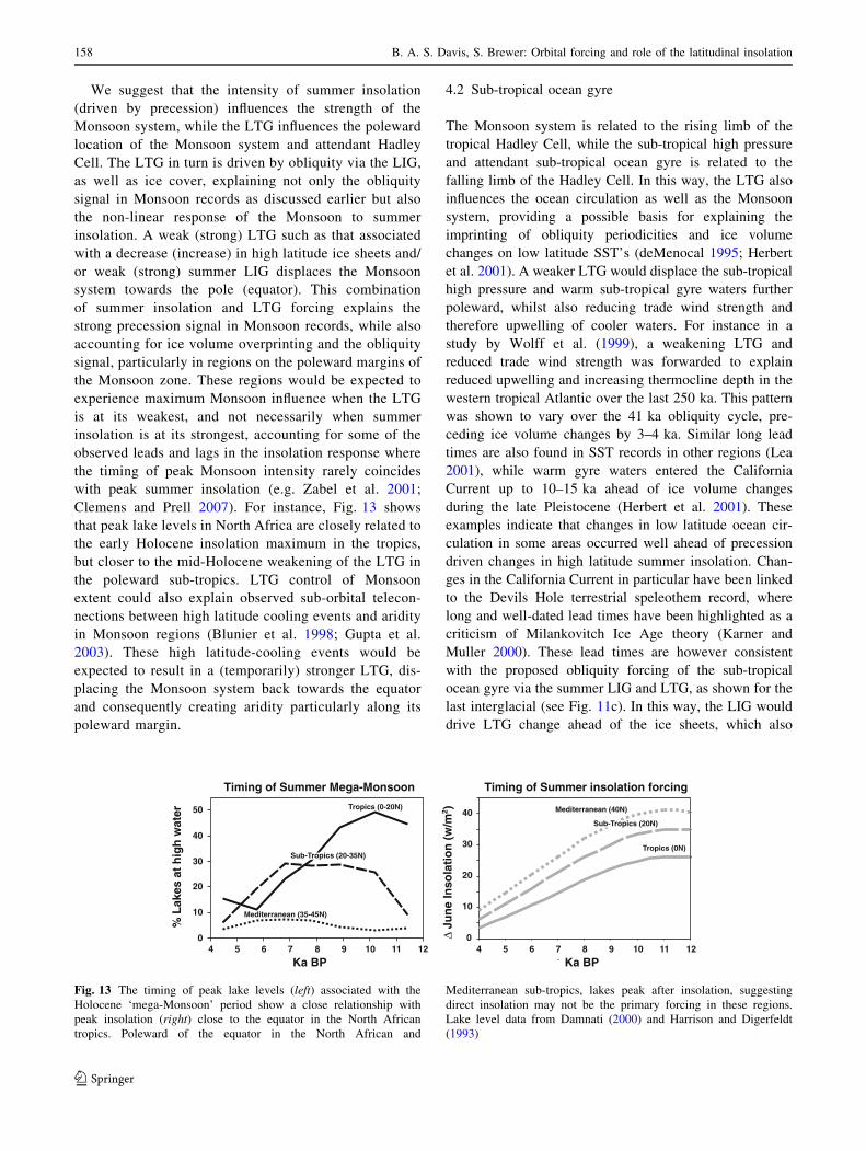
We suggest that the intensity of summer insolation

(driven by precession) influences the strength of the

Monsoon system, while the LTG influences the poleward

location of the Monsoon system and attendant Hadley

Cell. The LTG in turn is driven by obliquity via the LIG,

as well as ice cover, explaining not only the obliquity

signal in Monsoon records as discussed earlier but also

the non-linear response of the Monsoon to summer

insolation. A weak (strong) LTG such as that associated

with a decrease (increase) in high latitude ice sheets and/

or weak (strong) summer LIG displaces the Monsoon

system towards the pole (equator). This combination

of summer insolation and LTG forcing explains the

strong precession signal in Monsoon records, while also

accounting for ice volume overprinting and the obliquity

signal, particularly in regions on the poleward margins of

the Monsoon zone. These regions would be expected to

experience maximum Monsoon influence when the LTG

is at its weakest, and not necessarily when summer

insolation is at its strongest, accounting for some of the

observed leads and lags in the insolation response where

the timing of peak Monsoon intensity rarely coincides

with peak summer insolation (e.g. Zabel et al. 2001;

Clemens and Prell 2007). For instance, Fig. 13 shows

that peak lake levels in North Africa are closely related to

the early Holocene insolation maximum in the tropics,

but closer to the mid-Holocene weakening of the LTG in

the poleward sub-tropics. LTG control of Monsoon

extent could also explain observed sub-orbital telecon-

nections between high latitude cooling events and aridity

in Monsoon regions (Blunier et al. 1998; Gupta et al.

2003). These high latitude-cooling events would be

expected to result in a (temporarily) stronger LTG, dis-

placing the Monsoon system back towards the equator

and consequently creating aridity particularly along its

poleward margin.

4.2 Sub-tropical ocean gyre

The Monsoon system is related to the rising limb of the

tropical Hadley Cell, while the sub-tropical high pressure

and attendant sub-tropical ocean gyre is related to the

falling limb of the Hadley Cell. In this way, the LTG also

influences the ocean circulation as well as the Monsoon

system, providing a possible basis for explaining the

imprinting of obliquity periodicities and ice volume

changes on low latitude SST’s (deMenocal 1995; Herbert

et al. 2001). A weaker LTG would displace the sub-tropical

high pressure and warm sub-tropical gyre waters further

poleward, whilst also reducing trade wind strength and

therefore upwelling of cooler waters. For instance in a

study by Wolff et al. (1999), a weakening LTG and

reduced trade wind strength was forwarded to explain

reduced upwelling and increasing thermocline depth in the

western tropical Atlantic over the last 250 ka. This pattern

was shown to vary over the 41 ka obliquity cycle, pre-

ceding ice volume changes by 3–4 ka. Similar long lead

times are also found in SST records in other regions (Lea

2001), while warm gyre waters entered the California

Current up to 10–15 ka ahead of ice volume changes

during the late Pleistocene (Herbert et al. 2001). These

examples indicate that changes in low latitude ocean cir-

culation in some areas occurred well ahead of precession

driven changes in high latitude summer insolation. Chan-

ges in the California Current in particular have been linked

to the Devils Hole terrestrial speleothem record, where

long and well-dated lead times have been highlighted as a

criticism of Milankovitch Ice Age theory (Karner and

Muller 2000). These lead times are however consistent

with the proposed obliquity forcing of the sub-tropical

ocean gyre via the summer LIG and LTG, as shown for the

last interglacial (see Fig. 11c). In this way, the LIG would

drive LTG change ahead of the ice sheets, which also

0

10

20

30

40

4 5 6 7 8 9 10 11 12

Ka BP

Tropics (0N)

Mediterranean (40N)

Sub-Tropics (20N)Sub-Tropics (20N)

0

10

20

30

40

50

4 5 6 7 8 9 10 11 12

Ka BP

Tropics (0-20N)

Sub-Tropics (20-35N)Sub-Tropics (20-35N)

Mediterranean (35-45N)

Sub-Tropics (20-35N)

Timing of Summer Mega-Monsoon Timing of Summer insolation forcing

Sub-Tropics (20N)

∆ Ju

ne

Inso

lati

on

(w

/m2 )

% L

akes

at

hig

h w

ater

Fig. 13 The timing of peak lake levels (left) associated with the

Holocene ‘mega-Monsoon’ period show a close relationship with

peak insolation (right) close to the equator in the North African

tropics. Poleward of the equator in the North African and

Mediterranean sub-tropics, lakes peak after insolation, suggesting

direct insolation may not be the primary forcing in these regions.

Lake level data from Damnati (2000) and Harrison and Digerfeldt

(1993)


123

modify the obliquity signal. In the absence of large ice

sheets the obliquity signal would be expected to be stron-

ger, which may explain the strong obliquity signal found in

early Pleistocene California Current SST’s when large

Northern Hemisphere ice sheets had not yet developed (Liu

and Herbert 2004).

4.3 Mid-Pleistocene change from 41 to 100 ka cycles

The development of the Northern Hemisphere ice sheets in

the last 1.0–0.8 million years coincides with an important

shift from an Ice Age world dominated by 41 ka cycles, to

one dominated by 100 ka cycles. The origin of this shift

remains unclear, but ice volume changes appear closely

correlated with high latitude summer insolation over this

period (Fig. 1). This includes the observation that major

interglacials every 100 ka are generally coincident with

peaks in high latitude summer insolation caused by mod-

ulation of the 21 ka precession signal by the 100 ka

eccentricity cycle (Broecker 1992). Yet even Milankovitch

acknowledged that such orbital forcing alone would be too

weak to explain the observed climatic changes without

operating through amplifying feedbacks. One of the main

proposed feedbacks involves the ocean circulation, both

directly through surface and sub-surface (thermohaline)

heat transport (Imbrie et al. 1993), and indirectly through

its ability to store and release CO2 (Shackleton 2000;

Ruddiman 2003). However, what is less clear are how

changes in high latitude summer insolation could influence

the ocean system. We have already discussed possible

forcing of the sub-tropical ocean gyre through the summer

LIG and LTG, the season during which the sub-tropical

high pressure reaches its most poleward position. Warm

salty gyre waters are then carried to higher latitudes by the

mid-latitude westerly winds, which in the North Atlantic

form the North Atlantic Drift and Norwegian Current that

carry warm Gulf Stream waters far into Polar Regions.

But maximum ocean transport by this route occurs in

winter when the westerly winds are at their strongest, and

particularly under positive AO (NAO) conditions when

these winds have a greater southerly component that

directs warm air and ocean waters northwards (Blindheim

et al. 2000). The strong relationship between warm

Norwegian Sea SST’s, warm winters over Northern

Europe, a weak winter LTG and weak winter LIG sug-

gests LIG forcing of AO (NAO) type circulation that

would promote poleward ocean transport in this region.

This is essentially the same orbital forcing of the NAO as

proposed by Rimbu et al. (2004), based on winter tropical

insolation.

Changes in NAO (AO) associated with changes in LIG

could also have wider global implications because of the

strong advection of salty Atlantic waters into the Greenland

and Nordic Sea areas under positive NAO (AO) conditions.

This is because salty Atlantic waters in this region then

cool and sink to form a major source of North Atlantic

Deep Water (NADW) that drives the global thermohaline

circulation. The role of NADW formation in this area was

determined to be a critical factor in driving glacial–inter-

glacial cycles by Imbrie et al. (1992, 1993). In this case,

the authors saw the forcing coming from high latitude

summer insolation rather than the winter LIG, but there is

no contradiction in this because both forcings have almost

exactly the same orbital signature (compare Figs. 1b, 2b,

and Fig. 12a, c).

A further problem remains however in explaining the

non-linear response to insolation that has amplified the

100 ka signal since the mid-Pleistocene. This response has

been linked to the size of the continental ice sheets, which

appear to modify the response to insolation forcing through

a series of semi-stable states (Imbrie et al. 1993; Paillard

1998, 2001; Parrenin and Paillard 2003). Most of the major

changes in ice sheet size and distribution have occurred in

the North Atlantic region, which is also a key region for

determining the behaviour of the thermohaline circulation.

Bradley (1999, p 283) has therefore suggested that these

ice sheets, and particularly the Laurentide, could have

acted to significantly modify the westerly circulation as

they expanded and retreated, and in turn influenced the

North Atlantic ocean circulation. This mechanism could

therefore add a non-linear component to the control of the

mid-latitude westerly circulation and associated ocean

currents that we have proposed here operating through

linear changes in the winter LIG. This process may have

started with the formation of a large Greenland Ice Cap

around the mid-Pleistocene, when the first signs of NADW

formation started to appear in the Nordic Seas, and which

has been closely tied to the 100 ka cycle ever since

(Henrich et al. 2002). Certainly the Greenland Ice Cap

appears important in promoting local atmospheric forcing

of NADW formation in the Irminger Sea associated with a

positive NAO (AO) (Pickart et al. 2003), as well as

maintaining storm track strength and trajectory that cur-

rently carry warmth northward to the Barents Sea (Lunt

et al. 2004).

4.4 Maximum entropy production

LIG forcing of the LTG suggests a sensitivity of the cli-

mate system to small latitudinal variations in external solar

forcing that does not appear to be reproduced by today’s

climate models. The LTG in such models is not the func-

tion of any one simple theory, but the sum of complex local

and regional scale processes that determine the radiation

budget at each latitude (vegetation, clouds, sea ice, etc.),

as well as horizontal advective processes that move


123

energy between latitudes (Lindzen 1994). It therefore seems

remarkable that in a system composed of such strong and

independent internal processes, the LTG should be seen

here to be influenced by as weak an external forcing as the

LIG.

This surprising observation may therefore lend support

to the controversial theory that the LTG conforms to the

principle of maximum entropy production (MEP), and that

despite its complexity, the LTG is in fact finely balanced to

maximise entropy (Paltridge 1975; Whitfield 2005). If the

principle was robust enough, and the LTG was able to

remain in this steady state through time, then it could

follow that the LTG would vary only in response to weak

external forcing provided by the LIG, or very large internal

forcing such as ice sheets. The recent application of com-

plex GCM’s to investigate MEP has highlighted the use of

empirical estimates of boundary layer friction that appear

to underestimate the poleward energy flux in an MEP cli-

mate (Kleidon et al. 2003). This may provide some insight

into the apparent difficulty of GCM’s to reproduce suffi-

cient weakening of the mid-Holocene LTG shown here, as

well as LTG’s at other periods in the geological record

(Pierrehumbert 2002). It remains to be seen if MEP can

explain LIG forcing of the LTG, but it would appear that

the apparent lack of sensitivity to this forcing shown by

current climate models suggests a significant gap in our

present understanding of the climate system. This may

also be linked to the role of clouds and their interaction

with the large scale circulation, a factor that remains

one of the largest areas of uncertainty in modelling, and

which could significantly affect radiative forcing of surface

temperatures.

5 Conclusions

Changes in the Earth’s orbital precession and obliquity

influence the seasonal and latitudinal distribution of inso-

lation, but how this orbital forcing acts on the climate

system remains unclear. One of the key problems has been

understanding how strong obliquity signals can underlie

climatic changes commonly explained in terms of preces-

sion-driven variations in seasonal insolation, such as

glacial-interglacial cycles at high latitudes and the expan-

sion of the Monsoon system at low latitudes. A

reconstruction of the Northern Hemisphere LTG during the

Holocene shows that surface temperatures show an unex-

pectedly strong latitudinally dependant response to

insolation compared to climate models, which show a

stronger response to seasonal insolation. This unexpected

sensitivity of the LTG to the LIG may help explain the role

of obliquity, since in summer the LIG varies with obliquity.

The LTG in turn influences polar amplification of global

mean temperature (and hence high latitude warming),

while also influencing the poleward expansion of the

Hadley Cell and attendant Monsoon. In winter the LIG and

LTG vary with precession, and may therefore provide an

alternative explanation for precession signals in the palaeo-

climate record during a season when poleward heat and

moisture fluxes are at their highest. These seasonal dif-

ferences in the LIG–LTG response also appear to explain

differences in the timing of climatic changes between the

Holocene and the Eemain interglacials, which are other-

wise difficult to explain based on high latitude summer

insolation alone.

Our view of orbital forcing has been largely based on a

palaeoclimate record biased towards high latitudes and

the summer season. By improving our knowledge of

low latitudes and the winter season we may better under-

stand the complete seasonal and latitudinal response of the

climate system to insolation change, and in turn the

potential importance of the LIG and LTG in driving cli-

mate change.

Acknowledgments The contribution by Simon Brewer has been

funded in part by the EU MOTIF project (EVK2-2001-00263). We

acknowledge the PMIP international modeling groups for providing

their data for analysis and the Laboratoire des Sciences du Climat et

de l’Environnement (LSCE) for collecting and archiving the model

data. The PMIP2/MOTIF Data Archive is supported by CEA,

CNRS, the EU project MOTIF (EVK2-CT-2002-00153) and the

Programme National d’Etude de la Dynamique du Climat

(PNEDC). The analyses were performed using version 11-20-2005

of the database. More information is available on http://pmip2.

lsce.ipsl.fr/ and http://motif.lsce.ipsl.fr/. We also acknowledge the

resources of the NOAA World Data Centre for Paleoclimatology,

the PANGAEA Network for Geoscientific & Environmental Data

and the European Pollen Database. We would also like to thank

Odile Peyron and Carin Anderson for additional data, as well as

comments on early drafts by Jed Kaplan, Erin McClymont, Takeshi

Nakagawa and Tony Stevenson, as well as by two anonymous

referees.

Appendices

Appendix 1

Data sources and values for mid-Holocene SST data shown

in Fig. 3a, sorted first by proxy, then by latitude. The Basis

coding indicates how the 6 ka temperature anomaly was

calculated; (1) published linear regression equation, (2)

6 ± 0.5 ka reconstruction minus modern SST, (3)

6 ± 0.5 ka reconstruction minus 0 ± 0.5 ka reconstructed

SST. The Motif SST data was kindly supplied by Carin

Anderson. Pangaea data can be accessed at http://www.

pangaea.de. Original data has been used where ever pos-

sible, although sources depicted by (D) have been digitised

from published diagrams. Please refer to the source refer-

ence for the original references cited.


123

http://pmip2.lsce.ipsl.fr/

http://pmip2.lsce.ipsl.fr/

http://motif.lsce.ipsl.fr/

http://www.pangaea.de

http://www.pangaea.de

ecnerefeR lanigirOecruoSsisaBylamonAnosaeSyxorP.gnoL.taLeroC/etiS

M23258-2/3 75.00 13.97 Alkenone Summer 2.5 3 Marchal et al. 2002 Marchal et al. 2002 & Sarnthein et al. 20032002 .la te ovlaCaeagnaP33.1remmuSenoneklA36.779.66110259DM

2002 .la te lahcraMaeagnaP23.2launnAenoneklA69.52-67.85510259DMIOW225514 57.84 8.70 Alkenone Annual 2.8 1 Kim et al. 2004 Emeis et al. 2003

3002 .la te siemEfitoM27.4launnAenoneklA90.776.75715522WOIAD91-17 40.87 18.64 Alkenone Annual 2.6 1 Kim et al. 2004 Giunta et al. 2001M44-KL71 40.84 27.76 Alkenone Annual 0.9 1 Kim et al. 2004 Sperling et al. 2003

1002 .la te ohcaCfitoM29.2-launnAenoneklA85.3114.8383-97SBBS79-33 38.25 14.02 Alkenone Annual 1.5 1 Marchal et al. 2002 Cacho et al. 2001

0002 .la te draBfitoM26.0launnAenoneklA81.01-77.7381-18USdehsilbupnu siemE & 3002 noswaD dna siemEaeagnaP31.2launnAenoneklA91.3140.738CUM87/87LS-4-04M

0002 .la te siemEfitoM23.3launnAenoneklA27.7157.6311LRM39-008 36.38 -7.08 Alkenone Annual 0.8 1 Kim et al. 2004 Cacho et al. 2001GeoB 5901-2 36.38 -7.07 Alkenone Annual 0.9 1 Kim et al. 2004 Kim et al. 2004

9991 .la te ohcaCfitoM28.0launnAenoneklA26.2-41.63340259DM0002 .la te siemEfitoM29.0-launnAenoneklA37.2370.43D769PDO

GeoB 5844-2 27.71 34.68 Alkenone Annual -0.6 1 Kim et al. 2004 Arz et al. 20030002 .la te laconeMed & 5991 .la te oahZfitoM29.0launnAenoneklA85.81-57.02C856PDO

BOFS 31K 19.00 -20.17 Alkenone Annual 0.8 3 Chapman et al. 1996 Zhao et al. 1995 & Chapman et al. 1996ODP 723B 18.05 57.62 Alkenone Annual -0.6 2 Higginson et al 2004 (D) Higginson et al 200474KL 14.32 57.35 Alkenone Annual -0.2 1 Kim et al. 2004 Kim et al. 2004

9991 .la te nnamelhüRaeagnaP33.0-launnAenoneklA52.16-80.214-30053M4002 .la te miKaeagnaP35.0-launnAenoneklA59.1570.11509-39YT

ODP 1002C 10.71 -65.17 Alkenone Annual 0.0 1 Kim et al. 2004 Herbert and Shuffert 2000 & Peterson et al. 2000GeoB1007-4 -6.00 11.00 Alkenone Annual -0.4 3 Mulitza & Ruhlemann 2000 (D) Mulitza & Ruhlemann 2000

3991 .la te çoKaeagnaP33.4remmuSmotaiD25.61-54.9624812SPMD952011 66.97 7.63 Diatom Summer 3.0 3 Marchal et. al. 2002 (D) Koç et al. unpublished

2991 .la te çoKaeagnaP23.3remmuSmotaiD55.201.366/4-97MH3002 .la te niehtnraSfitoM24.1-remmuSmaroF79.3100.573/2-85232M

4002 .la te nesdunK & 0002 .la te noskiriEfitoM20.0remmuSmaroF50.91-22.7640-701MH3002 .la tenekkaborbesiR & 3002 .la te nossrednAfitoM27.0-remmuSmaroF36.779.66110259DM

4002 .la te nesdunK & 0002 .la te noskiriEfitoM28.2-remmuSmaroF98.71-09.6650-701MHNEAP4K 61.50 -24.17 Foram Summer 0.5 3 Marchal et. al. 2002 (D) Marchal et. al. 2002

2002 .la te lahcraMfitoM29.1remmuSmaroF69.52-67.85510259DM2991 ysselpuDfitoM27.0remmuSmaroF07.41-05.5522-78AN

2002 .la te lahcraMfitoM20.2remmuSmaroF53.82-86.45K71PAEN2002 .la te lahcraMfitoM20.0remmuSmaroF80.63-07.2520-77HC

CH69-09 41.76 -47.35 Foram Summer 0.7 1 Marchal et al. 2002 Labeyrie et al. 1999KET80-19 40.55 13.35 Foram Summer -6.0 3 Kallel et al. 1997 (D) Kallel et al. 1997KET80-03 38.82 14.50 Foram Summer -4.6 3 Kallel et al. 1997 (D) Kallel et al. 1997SU81-18 37.77 -10.18 Foram Summer -1.2 1 Marchal et al. 2002 Duplessy 1992

1002 .la te laconeMedaeagnaP39.3-remmuSmaroF85.81-57.02C856PDOBOFS 31K 19.00 -20.17 Foram Summer -1.6 3 Chapman et al. 1996 Chapman et al. 1996

2002 .la te nevloDaeagnaP29.0remmuSairaloidaR36.779.66110259DMV29-206 64.90 -29.28 Foram Summer 3.50 2 Ruddiman & Mix 1993 Kellog 1984 & Ruddiman & Mix 1993V28-14 64.78 -29.57 Foram Summer 1.40 2 Ruddiman & Mix 1993 Kellog 1984 & Ruddiman & Mix 1993K714-15 58.77 -25.95 Foram Summer 0.40 2 Ruddiman & Mix 1993 Ruddiman & Mix 1996V23-23 56.08 -44.55 Foram Summer -2.20 2 Ruddiman & Mix 1993 Ruddiman & Mix 1993V27-114 55.05 -33.07 Foram Summer 2.30 2 Ruddiman & Mix 1993 Ruddiman & Mix 1993RC9-225 54.98 -15.40 Foram Summer 1.70 2 Ruddiman & Mix 1993 Ruddiman et al 1977 & Ruddiman & Mix 1993V29-192K 54.27 -16.78 Foram Summer 0.20 2 Ruddiman & Mix 1993 Ruddiman & Mix 1993V23-81 54.25 -16.83 Foram Summer -0.50 2 Ruddiman & Mix 1993 Ruddiman et al 1977V27-20 54.00 -46.20 Foram Summer -1.10 2 Ruddiman & Mix 1993 Ruddiman & McIntyre 1984V23-82 52.58 -21.93 Foram Summer -1.10 2 Ruddiman & Mix 1993 Sancetta et al. 1973RC9-228 52.55 -18.75 Foram Summer 1.40 2 Ruddiman & Mix 1993 Ruddiman et al 1977K708-1 50.00 -23.75 Foram Summer 1.30 2 Ruddiman & Mix 1993 Ruddiman et al 1977V29-183K 49.13 -25.50 Foram Summer 2.60 2 Ruddiman & Mix 1993 Ruddiman & Mix 1993V30-101K 44.10 -32.50 Foram Summer -2.50 2 Ruddiman & Mix 1993 Ruddiman & Mix 1993V29-179 44.02 -24.53 Foram Summer 0.90 2 Ruddiman & Mix 1993 Ruddiman & McIntyre 1984 & Ruddiman & Mix 1993V30-97 41.00 -32.93 Foram Summer -1.00 2 Ruddiman & Mix 1993 Ruddiman & McIntyre 1984M12309-2 26.83 -15.12 Foram Summer -1.30 2 Ruddiman & Mix 1993 Thiede 1977M12392-1 25.17 -16.85 Foram Summer 1.50 2 Ruddiman & Mix 1993 Thiede 1977 & Mix et al. 1986A179-15 24.80 -75.93 Foram Summer -1.40 2 Ruddiman & Mix 1993 Kipp 1976M12310-4 23.50 -18.72 Foram Summer -0.50 2 Ruddiman & Mix 1993 Thiede 1977M12379-1 23.13 -17.75 Foram Summer -2.40 2 Ruddiman & Mix 1993 Thiede 1977V30-51K 19.87 -19.92 Foram Summer -2.90 2 Ruddiman & Mix 1993 Mix et al. 1986V30-49 18.43 -21.08 Foram Summer 1.40 2 Ruddiman & Mix 1993 Mix et al. 1986V28-127 11.65 -80.13 Foram Summer -0.80 2 Ruddiman & Mix 1993 Ruddiman & Mix 1993RC9-49 11.18 -58.58 Foram Summer -0.50 2 Ruddiman & Mix 1993 Be et al. 1976 & Mix et al. 1986V25-75 8.58 -53.17 Foram Summer -0.60 2 Ruddiman & Mix 1993 Mix et al. 1986V30-36 5.35 -27.32 Foram Summer 2.00 2 Ruddiman & Mix 1993 Mix et al. 1986V25-60 3.28 -34.83 Foram Summer -2.00 2 Ruddiman & Mix 1993 Mix et al. 1986RC13-189 1.87 -30.00 Foram Summer -0.70 2 Ruddiman & Mix 1993 Mix et al. 1986


123

Appendix 2

The relationship between sea level and Northern Hemi-

sphere ice cover during Termination I (Holocene) used to

infer ice cover from sea level during Termination II (Ee-

mian) in Figs. 10 and 11. The dashed line indicates the

estimated Eemian high stand which was higher than today

as a result of a reduced Greenland ice sheet.

-100

0

100

200

300

400

500

600

700-140-120-100-80-60-40-200

Relative Sea Level (m)

% Ic

e C

over

(Nor

ther

n H

emis

pher

e)

Appendix 3

Detail of Holocene pollen-climate reconstruction for

Mekelermeer in the Netherlands (Bohncke et al. 1988;

Bohncke and Wijmstra 1988; Bohncke 1991) shown in

Fig. 11f. Analysis is based on a modern analogue technique

using pollen pft scores as detailed in Davis et al. (2003).

Diagram shows loess smoother in bold. Pollen data and

chronology (calibrated) is from the European Pollen Database

(site #547), accessed with kind permission of the author.

-14

-10

-6

-2

2

-2

0

2

4

0 2 4 6 8 10 12

-4

°mra

wT)

C(

°dl

oc T)

C(

Ky B.P.

References

Aalbersberg G, Litt T (1998) Multiproxy climate reconstructions for

the Eemian and Early Weichselian. J Quaternary Sci 13:367–

390. doi :10.1002/(SICI)1099-1417(1998090)13:5\367::AID-

JQS400[3.0.CO;2-I

Baker A, Smart PL, Edwards RL (1995) Paleoclimate implications of

mass spectrometric dating of a British flowstone. Geology

23:309–312. doi :10.1130/0091-7613(1995)023\0309:PIOMSD

[2.3.CO;2

Berger A (1978) Long-term variations of daily insolation and

Quaternary climate changes. J Atmos Sci 35:2362–2367. doi

:10.1175/1520-0469(1978)035\2362:LTVODI[2.0.CO;2

Beyerle U, Rueedi J, Leuenberger M, Aeschbach-Hertig W, Peeters F,

Kipfer R, Dodo A (2003) Evidence for periods of wetter and

cooler climate in the Sahel between 6 and 40 ka BP derived

from groundwater. Geophys Res Lett 30(4):1173. doi:10.1029/

2002GL016310

Blindheim J, Borovkov V, Hansen B, Malmberg SA, Turrell WR,

Osterhus S (2000) Upper layer cooling and freshening in the

Norwegian Sea in relation to atmospheric forcing. Deep Sea

Res Part I Oceanogr Res Pap 47:655–680. doi:10.1016/S0967-

0637(99)00070-9

Blunier T, Chappellaz J, Schwander J, Dallenbach A, Stauffer B,

Stocker TF, Raynaud D, Jouzel J, Clausen HB, Hammer CU,

Johnsen SJ (1998) Asynchrony of Antarctic and Greenland

climate change during the last glacial period. Nature

394(6695):739–743. doi:10.1038/29447

Bohncke S (1991) Palaeohydrological changes in the Netherlands

during the last 13,000 years. Thesis, Vrije University, Amster-

dam, p 187

Bohncke S, Wijmstra L (1988) Reconstruction of late-glacial lake-

level fluctuations in the Netherlands based on palaeobotanical

analyses, geochemical results and pollen density data. Boreas

17:403–425

Bohncke S, Wijmstra L, Vanderwoude J, Sohl H (1988) The

lateglacial infill of three lake successions in the Netherlands:

regional vegetational history in relation to NW European

vegetational developments. Boreas 17:385–402

Broecker WS (1992) Upset for Milankovitch theory. Nature 359:779–

780. doi:10.1038/359779a0

Braconnot P, Joussaume S, de Noblet N, Ramstein G (2000) Mid-

Holocene and Last Glacial Maximum African monsoon changes

as simulated within the Palaeoclimate Modelling Intercompar-

ison Project. Global Planet Change 26:51–66. doi:10.1016/

S0921-8181(00)00033-3

Braconnot P, Harrison S, Joussaume CD, Hewitt A, Kitoh JE,

Kutzbach J, Liu Z, Otto-Bliesner B, Syktus J, Weber SL (2004)

Evaluation of PMIP coupled ocean–atmosphere simulations of

the mid-Holocene. In: Battarbee RW, Gasse F, Stickley CE (eds)

Past climate variability through Europe and Africa. Kluwer,

Dordrecht, pp 515–533

Braconnot P, Otto-Bliesner B, Harrison S, Joussaume S, Peterchmitt

J-Y, Abe-Ouchi A, Crucifix M, Fichefet T, Hewitt CD,

Kageyamal M, Kitoh A, Loutre M-F, Marti O, Merkel U,

Ramstein G, Valdes P, Weber L, Yu Y, Zhao Y (2007a) Results

of PMIP2 coupled simulations of the mid-Holocene and Last

Glacial Maximum—Part 1: experiments and large-scale features.

Climates Past 3:261–277

Braconnot P, Otto-Bliesner B, Harrison S, Joussaume S, Peterchmitt

J-Y, Abe-Ouchi A, Crucifix M, Fichefet T, Hewitt CD,

Kageyamal M, Kitoh A, Loutre M-F, Marti O, Merkel U,

Ramstein G, Valdes P, Weber L, Yu Y, Zhao Y (2007b) Results

of PMIP2 coupled simulations of the mid-Holocene and Last

Glacial Maximum—Part 2: feedbacks with emphasis on the

location of the ITCZ and mid- and high latitudes heat budgets.

Climates Past 3:279–296

Bradley R (1999) Paleoclimatology: reconstructing climates of

the quaternary, 2nd edn. Academic Press, pp 613, ISBN

012124010X


123

http://dx.doi.org/10.1029/2002GL016310

http://dx.doi.org/10.1029/2002GL016310

http://dx.doi.org/10.1016/S0967-0637(99)00070-9

http://dx.doi.org/10.1016/S0967-0637(99)00070-9

http://dx.doi.org/10.1038/29447

http://dx.doi.org/10.1038/359779a0

http://dx.doi.org/10.1016/S0921-8181(00)00033-3

http://dx.doi.org/10.1016/S0921-8181(00)00033-3

Chapman MR, Shackleton NJ, Zhao M, Eglinton G (1996) Faunal and

alkenone reconstructions of subtropical North Atlantic surface

hydrology and paleotemperature over the last 28 ka. Paleocea-

nography 11(3):343–357. doi:10.1029/96PA00041

Claussen M (2003) Simulation of Holocene climate change using

climate-system models. In: Mackay A, Battarbee R, Birks J,

Oldfield F (eds) Global change in the Holocene. Arnold

Publishers, ISBN 0 340 76223 3, pp 422–434

Clemens SC, Prell WL (2007) The timing of orbital-scale Indian

monsoon changes. Quat Sci Rev 26:275–278. doi:10.1016/

j.quascirev.2006.11.010

COHMAP members (1988) Climatic changes of the last 18,000 years.

Observations and model simulations. Science 241:1043–1052

Cortijo E, Lehman S, Keigwin L, Chapman M, Paillard D, Labeyrie L

(1999) Changes in meridional temperature and salinity gradients

in the North Atlantic Ocean (30�–72�) during the last interglacial

period. Paleoceanography 14(1):23–33

Cuffey KM, Marshall SJ (2000) Substantial contribution to sea-level

rise during the last interglacial from the Greenland ice sheet.

Nature 404(6778):591–594

Damnati B (2000) Holocene lake records in the Northern Hemisphere

of Africa. J Afr Earth Sc 31(2):253–262

Davis BAS, Brewer S, Stevenson ACS, Guiot J, Data contributors

(2003) The temperature of Europe during the Holocene recon-

structed from pollen data. Quat Sci Rev 22:1701–1716

deMenocal PB (1995) Plio-Pleistocene African climate. Science

270:53–59

Duplessy J-C, Ivanova E, Murdmaa I, Paterne M, Labeyrie L (2001)

Holocene paleoceanography of the northern Barents Sea and

variations of the northward heat transport by the Atlantic Ocean.

Boreas 30:2–16

Felis T, Lohmann G, Kuhnert H, Lorenz SJ, Scholz D, Patzold J,

Al-Rousan SA, Al-Moghrabi SM (2004) Increased seasonality in

Middle East temperatures during the last interglacial period.

Nature 429:164–168

Fleitmann D, Burns SJ, Mudelsee M, Neff U, Kramers J, Mangini A,

Matter A (2003a) Holocene forcing of the Indian monsoon

recorded in a stalagmite from Southern Oman. Science 300(5626):

1737–1739

Fleitmann D, Burns SJ, Neff U, Mangini A, Matter A (2003b)

Changing moisture sources over the last 330,000 years in

Northern Oman from fluid-inclusion evidence in speleothems.

Quatern Res 60:223–232

Flohn H (1965) Probleme der theoretischen Klimatologie. Naturwis-

senschaftliche Rundschau 10:385–392

Fronval T, Jansen E (1996) Rapid changes in ocean circulation and

heat flux In the Nordic seas during the last interglacial period.

Nature 383(6603):806–810

Gallup CD, Cheng H, Taylor FW, Edwards RL (2002) Direct

determination of the timing of sea level change during Termi-

nation II. Science 295(5553):310–313

Gallimore R, Jacob R, Kutzbach J (2005) Coupled atmosphere–

ocean–vegetation simulations for modern and mid-holocene

climates: role of extratropical vegetation cover feedbacks.

Climate Dynamics 25(7–8):755–776

Ganopolski A, Kubatzki C, Claussen M, Brovkin V, Petoukhov V

(1998) The influence of vegetation–atmosphere–ocean interac-

tion on climate during the mid-Holocene. Science 280(5371):

1916–1919

Gladstone RM, Ross I, Valdes PJ, Abe-Ouchi A, Braconnot P, Brewer S,

Kageyama M, Kitoh A, Legrande A, Marti O, Ohgaito R, Otto-

Bliesner B, Peltier WR, Vettoretti G (2006) Mid-Holocene NAO: a

PMIP2 model intercomparison. Geophys Res Lett 32(16):L16707

Gupta AK, Anderson DM, Overpeck JT (2003) Abrupt changes in the

Asian southwest monsoon during the Holocene and their links to

the North Atlantic Ocean. Nature 421(6921):354–357

Harrison S, Digerfeldt G (1993) European lakes as palaeohydrolog-

ical and palaeoclimatic indicators. Quatern Sci Rev 12:233–248

Haug GH, Hughen KA, Sigman DM, Peterson LC, R}ohl U (2001)

Southward migration of the Intertropical Convergence Zone

through the Holocene. Science 293:1305–1307

Hays JD, Imbrie J, Shackleton NJ (1976) Variation in the Earth’s

orbit: pacemaker of the ice ages. Science 194:1121–1132

Henrich R, Baumann K-H, Huber R, Meggers H (2002) Carbonate

preservation records of the past 3 Myr in the Norwegian-

Greenland Sea and the northern North Atlantic: implications for

the history of NADW production. Mar Geol 184:17–39

Herbert TD, Schuffert JD, Andreasen D, Heusser L, Lyle M, Mix A,

Ravelo AC, Stott LD, Herguera JC (2001) Collapse of the

California current during glacial maxima linked to climate

change on land. Science 293(5527):71–76

Higginson MJ, Altabet MA, Wincze L, Herbert TD, Murray DW

(2004) A solar (irradiance) trigger for millennial–scale abrupt

changes in the southwest monsoon? Paleoceanography 19:PA3015.

doi:10.1029/2004PA001,031

Howard WR (1997) A warm future in the past. Nature 388:418–419

Huntley B, Prentice IC (1988) July temperatures in Europe from

pollen data, 6000 years before present. Science 241:687–690

Imbrie J, Hays JD, Martinson DG, McIntyre A, Mix AC, Morley JJ,

Pisias NG, Prell WL, Shackleton NJ (1984) The orbital theory of

Pleistocene climate: support from a revised chronology of the

Marine del-18O record. In: Berger A, Imbrie J, Hays JD, Kukla

G, Saltzman B (eds) Milankovitch and Climate, Part 1. Reidel

Publishing Co., Dordrecht, pp 269–305

Imbrie J, Boyle EA, Clemens SC, Duffy A, Howard WR, Kukla G,

Kutzbach JE, Martinson DG, McIntyre A, Mix AC, Molfino B,

Morley JJ, Peterson LC, Pisias NG, Prell WL, Raymo ME,

Shackleton NJ, Toggweiler JR (1992) On the structure and origin

of major glaciation cycles, 1. Linear responses to Milankovitch

forcing. Paleoceanography 7:701–738

Imbrie J, Berger A, Boyle EA, Clemens SC, Duffy A, Howard WR,

Kukla G, Kutzbach J, Martinson DG, McIntyre A, Mix AC,

Molfino B, Morley JJ, Peterson LC, Pisias NG, Prell WL, Raymo

ME, Shackleton NJ, Toggweiler JR (1993) On the structure and

origin of major glaciation cycles, 2. The 100,000-year cycle.

Paleoceanography 8:699–735

Jain S, Lall U, Mann ME (1999) Seasonality and interannual

variations of Northern Hemisphere temperature: equator-to-pole

gradient and land-ocean contrast. J Clim 12:1086–1100

Jolly D, Harrison S, Damnati B, Bonnefille R (1998) Simulated climate

and biomes of Africa during the late Quaternary: comparison with

pollen and lake status data. Quatern Sci Rev 17:629–657

Joussaume S, Taylor KE, Braconnot P, Mitchell JFB, Kutzbach JE,

Harrison SP, Prentice IC, Broccoli AJ, Abe-Ouchi A, Bartlein

PJ, Bonfils C, Dong B, Guiot J, Herterich K, Hewitt CD, Jolly D,

Kim JW, Kislov A, Kitoh A, Moutre MF, Masson V, McAvaney

B, McFarlane N, de Noblet N, Peltier WR, Peterschmitt JY,

Pollard D, Rind D, Royer JF, Schlesinger ME, Syktus J,

Thompson S, Valdes V, Vettoretti G, Webb RS, Wyputta U

(1999) Monsoon changes for 5000 years ago: results of 18

simulations from the Paleoclimate Modeling Intercomparison

Project (PMIP). Geophys Res Lett 26:859–862. doi:10.1029/

1999GL900126

Karner DB, Muller RA (2000) A causality problem for Milankovitch:

Science 288:2143–2144

Kerwin MW, Overpeck JT, Webb RS, DeVernal A, Rind DH, Healy

RJ (1999) The role of oceanic forcing in mid-Holocene Northern

Hemispheric climatic change. Paleoceanography 14:200–210

Kim J-H, Rimbu N, Lorenz SJ, Lohmann G, Nam S-I, Schouten S,

Ruhlemann C, Schneider RR (2004) North Pacific and North

Atlantic sea-surface temperature variability during the Holocene.

Quat Sci Rev 23(20–22):2141–2154


123

http://dx.doi.org/10.1029/96PA00041

http://dx.doi.org/10.1016/j.quascirev.2006.11.010

http://dx.doi.org/10.1016/j.quascirev.2006.11.010

http://dx.doi.org/10.1029/2004PA001,031

http://dx.doi.org/10.1029/1999GL900126

http://dx.doi.org/10.1029/1999GL900126

Kleidon A, Fraedrich K, Kunz T, Lunkeit F (2003) The atmospheric

circulation and states of maximum entropy production. Geophys

Res Lett 30(23):2223

Kukla GJ (2000) The last interglacial. Science 287(5455):987–988

Kutzbach JE, Street-Perrott FA (1985) Milankovitch forcing of

fluctuations in the level of tropical lakes from 18 to 0 ka BP.

Nature 317:130–134

Kutzbach JE, Liu Z (1997) Response of the African monsoon to

orbital forcing and ocean feedbacks in the middle Holocene.

Science 278:440–443

Larrasoana JC, Roberts AP, Rohling EJ, Winklhofer M, Wehausen R

(2003) Three million years of monsoon variability over the

northern Sahara. Climate Dynamics 21:689–698

Lauritzen SE (1995) High-resolution paleotemperature proxy record

for the Last Interglaciation based on Norwegian speleothems.


Lea DW (2001) Ice Ages, the California Current and Devils Hole.

Science 293(5527):59–60

Lindzen RS (1994) Climate dynamics and global change. Ann Revue

Fluid Mech 26:353–378

Liu ZH, Herbert TD (2004) High-latitude influence on the eastern

equatorial Pacific climate in the early Pleistocene epoch. Nature

427(6976):720–723

Lourens LJ, Antonarakou A, Hilgen FJ, Van Hoof AAM, Vergnaud-

Grazzini C, Zachariasse WJ (1996) Evaluation of the Plio-

Pleistocene astronomical timescale. Paleoceanography 11(4):

391–413

Lourens LJ, Wehausen R, Brumsack HJ (2001) Geological constraints

on tidal dissipation and dynamical ellipticity of the Earth over

the past three million years. Nature 409:1029–1033

Loutre M-F, Pailard D, Vimeux F, Cortijo E (2004) Does the mean

annual insolation have the potential to change the climate? Earth

Planet Sci Lett 221:1–14

Lunt DJ, de Noblet-Ducoudre N, Charbit S (2004) Effects of a melted

greenland ice sheet on climate, vegetation, and the cryosphere.

Climate Dynamics 23(7–8):679–694

Luthi D, Le Floch M, Bereiter B, Blunier T, Barnola J-M, Siegenthaler U,

Raynaud D, Jouzel J, Fischer H, Kawamura K, Stocker TF (2008)

High-resolution carbon dioxide concentration record 650,000–

800,000 years before present. Nature 453:379–382

Marchal O, Cacho I, Stocker T, Grimalt JO, Calvo E, Martrat B,

Shackleton N, Vautravers M, Cortijo E, van Kreveld S,

Andersson C, Koc N, Chapman M, Sbaffi L, Duplessy J-C,

Sarnthein M, Turon J-L, Duprat J, Jansen E (2002) Apparent long-

term cooling of the sea surface in the northeast Atlantic and

Mediterranean during the Holocene. Quatern Sci Rev 21:455–483

Masson V, Cheddadi R, Braconnot P, Joussaume S, Texier S, PMIP-

participating-groups (1999) Mid-Holocene climate in Europe:

what can we infer from PMIP model-data comparisons ? Climate

Dynamics 15:163–182

Masson-Delmotte V, Jouzel J, Landais A, Stievenard M, Johnsen SJ,

White JWC, Werner M, Sveinbjornsdottir A, Fuhrer K (2005)

GRIP Deuterium Excess reveals rapid and orbital-scale changes

in Greenland Moisture Origin. Science 309(5731):118–121

Milankovitch M (1930) Mathematische Klimalehre und Astronomi-

sche Theorie der Klimaschwankungen. In: Koeppen W, Geiger R

(eds) Handbuch der Klimatologie. Gebrueeder Borntraeger,

Berlin, pp 1–176

Mitchell TD, Hulme M, New M (2002) Climate data for political

areas. Area 34:109–112 (Dataset reference CRU TS 2.0 available

at: http://www.cru.uea.ac.uk/*timm/grid/index.html)

Moritz RE, Bitz CM, Steig EJ (2002) Dynamics of recent change in

the Arctic. Science 297(5586):1497–1502

Mulitza S, Ruhlemann C (2000) African Monsoonal precipitation

modulated by interhemispheric temperature gradients. Quatern

Res 53:270–274

Nesje A, Lie Ø, Olaf Dahl S (2000) Is the North Atlantic Oscillation

reflected in Scandinavian glacier mass balance records? J

Quatern Sci 15(6):587–601

Nesje A, Matthews JA, Olaf Dahl S, Berrisford MS, Andersson C

(2001) Holocene glacier fluctuations of Flatebreen and winter-

precipitation changes in the Jostedalsbreen region, western

Norway, based on glaciolacustrine sediment records. The Holo-

cene 11(3):267–280

Parrenin F, Paillard D (2003) Amplitude and phase of glacial cycles

from a conceptual model. Earth Planet Sci Lett 214:243–250

Paillard D (1998) The timing of Pleistocene glaciations from a simple

multi-state climate model. Nature 391:378–381

Paillard D (2001) Glacial cycles: toward a new paradigm. Rev

Geophy 39(3):325–346

Paltridge GW (1975) Global dynamics and climate change: a system

of minimum entropy exchange. Q J Royal Meteorol Soc 101:

475–484

Peixoto JP, Oort AH (1992) Physics of climate. American Institute of

Physics, New York

Peltier RW (1994) Ice age paleotopography. Science 265(5169):195–201

Peyron O, Jolly D, Bonnefille R, Vincens A, Guiot J (2000) Climate

of East Africa 6000 14C Yr BP as inferred from pollen data.


Pickart RS, Spall MA, Ribergaard MH, Moore GWK, Milliff RF

(2003) Deep convection in the. Irminger Sea forced by the

Greenland tip jet. Nature 424:152–156

Pierrehumbert RT (2002) The hydrologic cycle in deep-time prob-

lems. Nature 419(6903):191–198

Raymo ME, Nisancioglu K (2003) The 41 ka world: Milankovitch’s

other unsolved mystery. Paleoceanography 18(1):1011

Reijmer CH, Van Den Broeke MR, Schelle MP (2002) Air parcel

trajectories and snowfall related to five deep drilling locations in

Antarctica based on the ERA-15 dataset. J Clim 15:1957–1968

Rimbu N, Lohmann G, Kim J-H, Arz HW, Schneider R (2003) Arctic/

North Atlantic Oscillation signature in Holocene sea surface

temperature trends as obtained from alkenone data. Geophys Res

Lett 30(6):1280

Rimbu N, Lohmann G, Lorenz SJ, Kim J-H, Schneider RR (2004)

Holocene climate variability as derived from alkenone sea

surface temperature and coupled ocean–atmosphere model

experiments. Climate Dynamics 23:215–227

Rind D (1998) Latitudinal temperature gradients and climate change.

J Geophys Res 103:5943–5971

Rossignol-Strick M, Nesteroff W, Olive P, Vergnaud-Grazzini C

(1982) After the deluge: Mediterranean stagnation and sapropel

formation. Nature 295:105–110

Rossignol-Strick M, Paterne M, Bassinot FC, Emeis K-C, de Lange

GJ (1998) An unusual mid-Pleistocene monsoon period over

Africa and Asia. Nature 392:269–272

Rousseau DD, Hatte Ch, Guiot J, Duzer D, Schevin P, Kukla G (2006)

Reconstruction of the Grande Pile Eemian using inverse

modeling of biomes and d13C. Quatern Sci Rev 25:2806–2819

Ruddiman WF (2003) Orbital insolation, ice volume, and greenhouse

gases. Quatern Sci Rev 22(15):1597–1629

Ruddiman WF (2006) What is the timing of orbital-scale monsoon

changes? Quatern Sci Rev 25(7–8):657–658

Ruddiman WF, Mix AC (1993) The North Atlantic and Equatorial

Atlantic at 9000 and 6000 yr B.P. In: Wright HE, Kutzbach JE,

Webb III T, Ruddiman WF, Street-Perrott FA, Bartlein PJ (eds)

Global climates since the last glacial maximum. Holocene

vegetation and climates of Europe. University of Minnesota

Press, Minnesota, pp 94–124

Sawada M, Viau AE, Vettoretti G, Peltier WR, Gajewski K (2004)

Comparison of North-American pollen-based temperature and

global lake-status with Ccma AGCM2 output at 6 ka. Quatern

Sci Rev 23:225–244


123

http://www.cru.uea.ac.uk/~timm/grid/index.html

Schrag DP (2000) Climatology: of ice and elephants. Nature

404(6773):23–24

Shackleton NJ (2000) The 100,000-year ice-age cycle identified and

found to lag temperature, carbon dioxide, and orbital eccentric-

ity. Science 289:1897–1902

Spotl C, Mangini A, Frank N, Eichstadter R, Burns SJ (2002) Start of

the last interglacial period at 135 ka: evidence from a high

Alpine speleothem. Geology 30(9):815–818

Thompson DWJ, Wallace JM (1999) Annular modes in the

extratropical circulation. Part I: month-to-month variability. J

Clim 13(5):1000–1016. Data available from: http://www.atmos.

colostate.edu/ao/Data/ao_index.html

Torrence C, Compo GP (1998) A practical guide to wavelet analysis.

Bull Am Meteorol Soc 79:61–78

Tzedakis C (2003) Timing and duration of last interglacial conditions

in Europe: a chronicle of a changing chronology. Quatern Sci

Rev 22:763–768

Valdes P (2003) An introduction to climate modelling of the

Holocene. In: Mackay A, Battarbee R, Birks J, Oldfield F

(eds) Global change in the Holocene. Arnold Publishers, ISBN 0

340 76223 3, pp 20–35

Vimeux F, Masson V, Jouzel J, Stievenard M, Petit JR (1999) Glacial-

interglacial changes in ocean surface conditions in the Southern

Hemisphere. Nature 398(6726):410–413

Visbeck M (2002) The Ocean’s role in Atlantic climate variability.

Science 297(5590):2223–2224

Waelbroeck C, Labeyrie L, Michel E, Duplessy JC, McManus JF,

Lambeck K, Balbon E, Labracherie M (2002) Sea-level and deep

water temperature changes derived from benthic foraminifera

isotopic records. Quatern Sci Rev 21:295–305

Whitfield J (2005) Order out of chaos. Nature 436(7053):905–907

Winograd IJ (2002) The California current, Devils hole, and

Pleistocene climate. Science 296:7

Winograd IJ, Coplen TB, Landwehr JM, Riggs AC, Ludwig KR,

Szabo BJ, Kolesar PT, Revesz KM (1992) Continuous 500,000-

year climate record from vein calcite in Devils Hole, Nevada.

Science 258:255–260

Wolff T, Mulitza S, Ruhlemann C, Wefer G (1999) Response of the

tropical Atlantic thermocline to late Quaternary trade wind

changes. Paleoceanography 14(3):374–383

Young MA, Bradley RS (1984) Insolation gradients and the

paleoclimatic record. In: Berger AL et al (eds) Milankovitch

and climate Part 2. D. Reidel, Norwell, pp 707–713

Zabel M, Schneider RR, Wagner T, Adegbie AT, de Vries U, Kolonic S

(2001) Late Quaternary climate changes in Central Africa as inferred

from terreginous input to the Niger Fan. Quatern Res 56:207–217

Zachos J, Pagani M, Thomas E, Billups K (2001) Trends, rhythms,

and aberrations in global climate 65 Ma to present. Science

292:686–693

Zagwijn WH (1996) An analysis of Eemian climate in western and

central Europe. Quatern Sci Rev 15:451–469

Zhao Y, Braconnot P, Marti O, Harrison SP, Hewitt C, Kitoh A, Liu

Z, Mikolajewicz U, Otto-Bliesner B, Weber SL (2005) A multi-

model analysis of role of ocean feedback on the African and

Indian monsoon during Mid-Holocene. Clim Dyn 25:777–800.

doi:10.1007/s00382-005-0075-7


123

http://www.atmos.colostate.edu/ao/Data/ao_index.html

http://www.atmos.colostate.edu/ao/Data/ao_index.html

http://dx.doi.org/10.1007/s00382-005-0075-7

orbital forcing and role of the latitudinal insolation ... · periodicities in the...

Documents