glacial-interglacial atmospheric co2 change: a possible “standing

Clim. Past, 5, 537–550, 2009www.clim-past.net/5/537/2009/© Author(s) 2009. This work is distributed underthe Creative Commons Attribution 3.0 License.

Climateof the Past

Glacial-interglacial atmospheric CO2 change: a possible “standingvolume” effect on deep-ocean carbon sequestration

L. C. Skinner

Godwin Laboratory for Palaeoclimate Research, Dept. of Earth Sciences, Univ. of Cambridge, Cambridge, CB2 3EQ, UK

Received: 8 April 2009 – Published in Clim. Past Discuss.: 4 May 2009Revised: 1 August 2009 – Accepted: 4 September 2009 – Published: 30 September 2009

Abstract. So far, the exploration of possible mechanismsfor glacial atmospheric CO2 drawdown and marine carbonsequestration has tended to focus on dynamic or kinetic pro-cesses (i.e. variable mixing-, equilibration- or export rates).Here an attempt is made to underline instead the possible im-portance of changes in the standing volumes of intra-oceaniccarbon reservoirs (i.e. different water-masses) in influenc-ing the total marine carbon inventory. By way of illustra-tion, a simple mechanism is proposed for enhancing the ma-rine carbon inventory via an increase in the volume of rel-atively cold and carbon-enriched deep water, analogous tomodern Lower Circumpolar Deep Water (LCDW), filling theocean basins. A set of simple box-model experiments con-firm the expectation that a deep sea dominated by an ex-panded LCDW-like watermass holds more CO2, without anypre-imposed changes in ocean overturning rate, biologicalexport or ocean-atmosphere exchange. The magnitude ofthis “standing volume effect” (which operates by boostingthe solubility- and biological pumps) might be as large as thecontributions that have previously been attributed to carbon-ate compensation, terrestrial biosphere reduction or oceanfertilisation for example. By providing a means of not onlyenhancing but also driving changes in the efficiency of thebiological- and solubility pumps, this standing volume mech-anism may help to reduce the amount of glacial-interglacialCO2 change that remains to be explained by other mecha-nisms that are difficult to assess in the geological archive,such as reduced mass transport or mixing rates in particular.This in turn could help narrow the search for forcing con-ditions capable of pushing the global carbon cycle betweenglacial and interglacial modes.

Correspondence to:L. C. Skinner([email protected])

1 Explaining glacial-interglacial CO2 change

Although it is clear that changes in atmospheric CO2 have re-mained tightly coupled with global climate change through-out the past∼730 000 years at least (Siegenthaler et al.,2005), the mechanisms responsible for pacing and moder-ating CO2 change remain to be proven. The magnitude ofthe marine carbon reservoir, and its inevitable response tochanges in atmospheric CO2 (Broecker, 1982a), guaranteesa significant role for the ocean in glacial-interglacial CO2change. Based on thermodynamic considerations, glacialatmospheric CO2 would be reduced by∼30 ppm simplydue to the increased solubility of CO2 in a colder glacialocean (Sigman and Boyle, 2000); however this reductionwould be counteracted by the reduced solubility of CO2in a more saline glacial ocean and by a large reduction inthe terrestrial biosphere under glacial conditions (Broeckerand Peng, 1989; Sigman and Boyle, 2000). The bulk ofthe glacial-interglacial CO2 change therefore remains to beexplained by more complex inter-reservoir exchange mech-anisms, and the most viable proposals involve either thebiological- or the physical “carbon pumps” of the ocean. Onthis basis, any mechanism that is invoked to explain glacial-interglacial CO2 change must involve changes in the seques-tration of CO2 in the deepest marine reservoir (Broecker,1982a; Boyle, 1988a, 1992; Broecker and Peng, 1989).

To date, three main types of conceptual model have beenadvanced in order to explain glacial-interglacial atmosphericCO2 change: (1) those involving an increase in the exportrate of organic carbon to the deep sea, either via increasednutrient availability at low latitudes or via increased effi-ciency of nutrient usage at high latitudes (Broecker, 1982a,b; Knox and McElroy, 1984); (2) those involving a reduc-tion in the “ventilation” of water exported to the deep South-ern Ocean (Siegenthaler and Wenk, 1984; Toggweiler andSarmiento, 1985), either via sea-ice “capping” (Keeling andStephens, 2001) or a change in the surface-to-deep mixingrate/efficiency (Toggweiler, 1999; Gildor and Tziperman,

Published by Copernicus Publications on behalf of the European Geosciences Union.

http://creativecommons.org/licenses/by/3.0/

538 L. C. Skinner: Standing volume effects on CO2

2001; Watson and Naveira Garabato, 2006); and (3) thoseinvolving changes in whole ocean chemistry and “carbonatecompensation”, possibly promoted by changes in the ratio oforganic carbon and carbonate fluxes to the deep sea. (Archerand Maier-Reimer, 1994). Each of these conceptual mod-els has its own set of difficulties in explaining the patternand magnitude of past glacial-interglacial CO2 change, andin fact none is likely to have operated in complete isolation(Archer et al., 2000; Sigman and Boyle, 2000). Neverthe-less, one aspect of all of the proposed models that emergesas being fundamental to any mechanism proposing to explainglacial-interglacial CO2 change is the balance between bio-logical carbon export from the surface-ocean and the returnof carbon to the surface by the ocean’s overturning circula-tion. These two processes, one biological and one physical,essentially determine the balance of carbon input to and out-put from (and therefore the carbon content of) the deepestmarine reservoirs (Toggweiler et al., 2003).

The regions of deep-water formation in the North Atlanticand especially in the Southern Ocean play a key role in set-ting the “physical side” of this balance. In the North Atlantic,carbon uptake via the “solubility pump” is enhanced by thelarge temperature change that surface water must undergobefore being exported into the ocean interior. The forma-tion of North Atlantic deep-water therefore represents an effi-cient mechanism for mixing CO2 deep into the ocean interior(Sabine et al., 2004); though only to the extent that it is notcompletely compensated for (or indeed over-compensatedfor) by the eventual return flow of more carbon-enricheddeep-water back to the surface (Toggweiler et al., 2003). Ar-guably, it is in controlling the extent to which the return flowof deep-water to the surface (which occurs primarily in theSouthern Ocean) represents an effective ‘reflux’ of carbonto the atmosphere, acting against biological export, that theformation of deep-water in the Southern Ocean plays a piv-otal role in controlling the partitioning of CO2 between thesurface- and the deep ocean. We might say that if the south-ern overturning loop “leaks” too much, it will be an efficientcarbon source to the atmosphere (Toggweiler et al., 2003);and if it does not leak much, it will simply become a largestanding carbon reservoir. The degree to which the south-ern overturning loop “leaks” depends on the efficiency ofequilibration of up-welled Southern Ocean deep-water withthe atmosphere, relative to the efficiency of carbon export(dissolved and particulate) from the surface Southern Ocean(Toggweiler, 1999; Gildor and Tziperman, 2001).

Today, a significant portion of the deep ocean (althoughnot the deep Atlantic – “deep” meaning greater than∼1 kmin this context) is filled from the Southern Ocean by LowerCircumpolar Deep Water (LCDW) that is exported north-wards into the various ocean basins from the eastward cir-culating Antarctic Circumpolar Current (ACC) (Orsi et al.,1999; Sloyan and Rintoul, 2001). This deep-water remainsrelatively poorly equilibrated with the atmosphere and is in-efficiently stripped of its nutrients, thus maintaining an ele-

vated “pre-formed” nutrient and dissolved inorganic carboncontent. In part this is because of the very low tempera-ture at which deep-water forms around Antarctica and be-cause the rate of ocean – atmosphere CO2 exchange can-not keep up with the rate of overturning in the uppermostSouthern Ocean (Bard, 1988). However it is primarily be-cause the bulk of southern sourced deep- and bottom-wateris either produced via a combination of brine rejection be-low sea-ice and entrainment from the sub-surface, or con-verted from “aged” northern-sourced deep-waters that feedinto the Southern Ocean via Upper Circumpolar Deep Wa-ter (UCDW) (Orsi et al., 1999; Speer et al., 2000; Webb andSuginohara, 2001; Sloyan and Rintoul, 2001). Intense turbu-lent mixing around topographic features in the deep SouthernOcean helps to enhance the amount of “carbon rich” sub-surface water that is incorporated into LCDW (from UCDWabove and from Antarctic Bottom Water, AABW, below),and that is subsequently exported northwards to the Atlanticand Indo-Pacific (Orsi et al., 1999; Naviera Garabato et al.,2004). The process of Lower Circumpolar Deep Water ex-port in the deep Southern Ocean (as distinct from deep-waterformation in the North Atlantic, and the vertical mixing inthe uppermost Southern Ocean) can therefore be viewed as amechanism that helps to “recycle” carbon-rich water withinthe ocean interior, circumventing ocean – atmosphere ex-change, and eventual CO2 leakage to the atmosphere.

It is notable that nearly all of the “physical pump” mech-anisms that have been proposed as significant controls onglacial-interglacial CO2 change have referred to dynamical(export- or mixingrate) or kinetic (ocean – atmosphere ex-changerate) effects (e.g. Kohler et al., 2005; Toggweiler,1999; Tziperman and Gildor, 2003; Brovkin et al., 2007;Peacock et al., 2006; Sigman and Haug, 2003). Consider-ation of the effect on atmospheric CO2 of changes in the ge-ometry, and therefore thevolumes, of different intra-oceaniccarbon reservoirs (i.e. different deep-water “masses”) haslargely escaped explicit treatment. This is surprising, giventhat the residence time of a reservoir will scale inversely toits renewal rate or positively to its volume. It is also surpris-ing from an “experimental” perspective, given that most ofthe palaeoceanographic evidence available to us can tell ussomething about changes in water-mass distribution (hencevolume), but usually cannot tell us much about changes incirculation or mixing rates. Furthermore, if we consider whatcontrols the energy and buoyancy budgets of the ocean (andhence the capacity to maintain an overturning circulation),it is not obvious that the net overturningrate of the oceanmust have been significantly different from modern over longtime periods in the past (Gordon, 1996; Wunsch, 2003) –even if it is true that the reconstructed hydrography of theglacial ocean is inconsistent with the modern circulation (es-pecially in terms of vertical property distributions) (Marchaland Curry, 2008). The circulation rate (mass transport) of theglacial ocean therefore remains poorly constrained, despitewell-defined property distribution (hence inventory) changes.

Clim. Past, 5, 537–550, 2009 www.clim-past.net/5/537/2009/

L. C. Skinner: Standing volume effects on CO2 539

The purpose of the present study is to focus attention onthe importance of distinguishing between past changes in thedistribution of water-masses (which we can know somethingabout) and past changes in their renewal rates (which we tendto know very little about), in particular when considering therole of the ocean circulation in setting the marine carbon in-ventory. By way of illustration, the simple hypothesis is ad-vanced that the amount of carbon that can be “bottled up” inthe deep ocean may be significantly affected by changes inthe volumesof different glacial deep-water masses, prior toany imposed changes in overturning-, gas exchange- or bio-logical exportrates(but including the effects of any redistri-bution of temperature, salinity, and pre-formed/remineralisednutrients that is incurred). Of course, the suggestion is notthat changes in circulation- or export rates are unimportant;but rather that they are not exclusively important. The dis-tinction between these two aspects of the ocean circulation(i.e. water-mass distributionversusoverturning rate), and theevaluation of their individual impacts on atmospheric CO2,could prove to be important in assessing the mechanisms ofglacial-interglacial CO2 change, in particular if it is possi-ble for these two aspects of the ocean circulation to becomedecoupled, for example on long time-scales or for specificforcing. Put another way: if the mechanisms or time-scalesrequired to alter the marine carbon inventory via changes inoverturning rates and water-mass volumes differ, then theycannot be usefully conflated in the single term “ocean cir-culation” when considering the causes of glacial-interglacialCO2 change.

In this paper additional emphasis is placed on how the hyp-sometry of the ocean basins (the area distribution at differentwater depths) may affect the efficiency of volumetric water-mass changes that are caused by the shoaling/deepening ofwater-mass mixing boundaries. A notable fact in this regardis that∼56% of the sea-floor lies between 6000 and 3000 m(Menard and Smith, 1966), thus accounting for a majorityincrement in the ocean’s volume. If a water mass that onceoccupied the>5 km interval in the Atlantic comes to occupythe>2 km interval, it will have increased its volume in thisbasin almost four-fold.

2 A thought experiment: a “southern flavour ocean”

Arguably, one of the least ambiguous aspects of the palaeo-climate archive is the record of glacial-interglacial changein δ13C recorded by benthic foraminifera from the AtlanticOcean (Curry and Oppo, 2005; Duplessy et al., 1988). Thedata suggest, at the Last Glacial Maximum, a more positiveδ13C of DIC in the upper∼2 km of the Atlantic, and a morenegativeδ13C of dissolved inorganic carbon (DIC) belowthis in the deepest Atlantic. These data do not appear to beconsistent with the modern water-mass geometry/circulation(Marchal and Curry, 2008). The most widespread and well-supported interpretation of these data is that they represent

a redistribution of glacial northern- and southern-sourceddeep and intermediate water-masses, including in particu-lar an incursion of glacial southern-sourced deep water (richin preformed and remineralised nutrients, and of lowδ13C)into the deep North Atlantic, up to a water depth of∼2–3 km (Curry et al., 1988; Duplessy et al., 1988; Oppo andFairbanks, 1990; Oppo et al., 1990; Boyle, 1992; Curryand Oppo, 2005; Hodell et al., 2003). This interpreta-tion is now strongly supported by glacial Atlantic benthicforaminiferal Cd/Ca, Zn/Ca and B/Ca ratios (Marchitto andBroecker, 2005; Boyle, 1992; Keigwin and Lehmann, 1994;Marchitto et al., 2002; Yu and Elderfield, 2007). Auxiliarysupport has been provided by benthic radiocarbon measure-ments from the North Atlantic (Robinson et al., 2005; Skin-ner and Shackleton, 2004; Keigwin, 2004), and neodymiumisotope measurements (εNd ) from the South Atlantic (Rut-berg et al., 2000; Piotrowski et al., 2005, 2004). An ele-gant box-model investigation of the possible causes of glacialdeep-ocean chemistry (Michel et al., 1995) and coupledatmosphere-ocean general circulation model (AOGCM) sim-ulations of the “last glacial maximum” circulation (e.g. Shinet al., 2003; Kim et al., 2003) have also added weight to thisinterpretation of glacial deep-water mass geometry. If weassume that the relationships between deep-water radiocar-bon activity, carbonate ion concentration,δ13C of DIC andTCO2 remained similar between glacial and interglacial (pre-industrial) times, at least for deep-water exported northwardsfrom the Southern Ocean, then we may also infer that the wa-ter that apparently replaced NADW in the Atlantic and dom-inated LCDW export to the Indo-Pacific basins was also ofrelatively high TCO2. Indeed, radiocarbon evidence (Mar-chitto et al., 2007), dissolution indices (Barker et al., 2009),benthicδ13C (Ninneman and Charles, 2002; Hodell et al.,2003) and pore-water temperature/salinity estimates (Adkinset al., 2002) all tend to suggest that deep-water exported fromthe Southern Ocean during the last glacial would have repre-sented a concentrated and isolated carbon reservoir that wasvery poorly equilibrated with the atmosphere.

Given these constraints on the deep-water hydrographynear the height of the last glaciation (Lynch-Steiglitz et al.,2007), one question immediately arises: how much mustthe volumeof southern-sourced deep-water (LCDW) haveincreased, regardless of its exportrate, in order to accom-plish the observed change (i.e. filling the deep Atlantic, anddominating the deep-water export to the Indian and Pacificbasins)? Further, and more importantly, what would havebeen the immediate effect on deep-water CO2 sequestration,if any, of the resulting redistribution of dissolved inorganiccarbon, nutrients and temperature/salinity? Answering thefirst question is straightforward enough: as noted above,based on the hypsometry of the Atlantic basin (Menardand Smith, 1966), raising the upper boundary of southern-sourced deep-water (assumed for the sake of argument tobe approximately flat) from 5 km to 2.5 km in the Atlanticrequires this water-mass to increase its Atlantic volume from

www.clim-past.net/5/537/2009/ Clim. Past, 5, 537–550, 2009


under 20 million km3 to nearly 70 million km3 (just under a4-fold increase). In order to determine the eventual impact ofthis volumetric change on the carbon-storage capacity of theocean we would obviously require knowledge of the chang-ing chemistry of the various deep-water masses in the oceanas well as their turnover and “ventilation” (atmosphere equi-libration) rates, and the flux of dissolved carbon that theyeventually incorporate via biological export. However, if weassume simplistically that nothing in the ocean changes ex-cept the volume occupied by southern-sourced deep-water(i.e. the chemistry of all water-masses stays the same, butnot their volumetric contribution to the ocean’s total bud-get), then we can infer that for a 4-fold increase in the vol-ume of AABW at the expense of NADW (having averagetotal dissolved CO2 concentrations of∼2280µmol kg−1 and∼2180µmol kg−1, respectively, Broecker and Peng, 1989)the ocean would need to gain∼63 Gt of carbon. If we assumethat all this carbon must come from the atmosphere, thenatmosphericpCO2 would have to drop by∼30 ppm, given1 ppm change per 2.12 Gt carbon removed from the atmo-sphere (Denman et al., 2007). This is equivalent to∼38% ofthe total observed glacial-interglacial CO2 change (Siegen-thaler et al., 2005), and is comparable to the magnitude ofatmospheric CO2 changes that are likely to have arisen fromother viable mechanisms such as biological export increase,or carbonate compensation (Peacock et al., 2006).

Clearly many of the assumptions made in the abovethought experiment might not be valid: the chemistry anddynamics, not to mention the character and rate of biologicalexport, of the glacial ocean will probably not have remainedconstant. Nevertheless, palaeoceanographic proxy evidenceholds that the basic premise of the thought experiment isvalid: the volume of deep water closely resembling mod-ern southern-sourced deep-water apparently increased signif-icantly during the last glaciation. It seems warranted there-fore to evaluate the impacts of this premise in a slightly moresophisticated way. The question to be answered is: doesa deep ocean dominated by a LCDW-like water-mass holdmore carbon at steady state (on time-scales longer than themixing time of the ocean)? Below, a very simple box modelis used as a first step toward answering this question.

3 Box-model description

Figure 1 illustrates a simple box-model that has been con-structed in order to explore in more detail the implica-tions of deep-water mass geometry (versusoverturning rate)changes for glacial-interglacial CO2 variability. This modelcomprises an atmosphere and six ocean boxes (SouthernOcean, low-latitude, North Atlantic, northern deep water,intermediate-water and southern deep water), and involvestwo coupled circulation cells with down welling in the south-ern and northern high latitudes. Geological exchange of min-erals and nutrients (river alkalinity input, sedimentation, car-

Standing volume effects on CO2

23

Figures

Figure 1

Fig. 1. Box-model schematic (S, southern surface; L, low-latitude surface; N, northern surface; ND, north deep; Int, intermediate; SD, south deep). The vertical dashed line is intended to suggest an alternative hypothetical box geometry, where southern sourced water dominates the deep ocean. Heavy black lines indicate thermohaline circulation (Fn =

northern overturning; Fs = southern overturning). Red arrows indicate two-way exchange (i.e.mixing) terms. Blue arrows indicate gas exchange. Grey arrows indicate particle fluxes. The particle fluxes Pi(sd) and Pi(nd) that by-pass the intermediate box from the low-latitude box are calculated in proportion to the volume of each deep box relative to the total deep ocean in the model, such that if Vnd/Vd = f, Pi(nd) = f x 0.1 x Pl and Pi(sd) = (1-f ) x 0.1 x Pl. Approximate box

depths are indicated at left (surface areas are given in Table 1).

Pl

Ps

Gl

SD

Fs

S

Int

L N

ND

Fn

(Fs+Fn)

Pn

Pi(nd)Pi(sd)

fni

fns

fli

AtmosphereGs Gn

fsi

0m

100m

1500m

2500m

4000m

Fig. 1. Box-model schematic (S, southern surface; L, low-latitudesurface; N, northern surface; ND, north deep; Int, intermediate; SD,south deep). The vertical dashed line is intended to suggest an al-ternative hypothetical box geometry, where southern sourced wa-ter dominates the deep ocean. Heavy black lines indicate thermo-haline circulation (Fn=northern overturning; Fs=southern overturn-ing). Red arrows indicate two-way exchange (i.e. mixing) terms.Blue arrows indicate gas exchange. Grey arrows indicate particlefluxes. The particle fluxes Pi(sd) and Pi(nd) that by-pass the inter-mediate box from the low-latitude box are calculated in proportionto the volume of each deep box relative to the total deep ocean inthe model, such that if Vnd/Vd=f, Pi(nd)=f×0.1×Pl and Pi(sd)=(1-f)×0.1×Pl. Approximate box depths are indicated at left (surfaceareas are given in Table 1).

bonate compensation) is not included in this model. Particlefluxes are treated as directly exported dissolved matter, withcarbon and phosphate being exported in fixed proportions, asdefined by modified Redfield Ratios (C:N:P:O2=130:16:1:-169) (Toggweiler and Sarmiento, 1985), and carbonate be-ing exported in fixed proportion to the TCO2 of the water.Particle fluxes are diagnosed for a baseline “pre-industrial”box-model scenario according to observed phosphate con-centrations in the modern ocean (Najjar et al., 1992):

P =C∗

P ∗

(([PO4] − [PO4] mod )V

τ

)whereP is the instantaneous organic carbon flux,C∗/P ∗ isthe ratio of organic carbon to phosphate in the particulatematter,V is the box volume,τ is the restoring time-scale (setto 0.1 year), and [PO4] and [PO4]mod are the instantaneousand restoring phosphate concentrations, respectively. In sub-sequent “altered” box-model scenarios, particle fluxes varyaccording to “Michaelis-Menton” type dynamics (Dugdale,1967), with less export being supported by lower nutrientconcentrations. This removes the possibility of unrealisti-cally high/low export productivity for very low/high nutrientlevels respectively:

P =C∗

P ∗

(ω[PO4]

km + [PO4]

)



In the above equation,km is set to 2.5 e−4 mol m−3 (Schulzet al., 2001), andω (the biological uptake rate) is diagnosedfrom the equilibrium conditions for the “modern box-modelscenario” (preceding equation).

The calculated components of the model include phos-phate, alkalinity, total dissolved CO2 (TCO2), carbonateion (CO2−

3 ), pCO2, apparent oxygen utilisation (AOU) andnormalised radiocarbon concentration (114C). Because themodelled radiocarbon concentrations are not normalisedwith respect toδ13C, 114C reported here is actually equiv-alent to d14C by definition (Stuiver and Polach, 1977). Ide-alised mass-balance equations for the evolution of box con-centrations are of the form:

Vn

dCn

dt=Fn(Cl−Cn)+fni(Ci−Cn)−Pn

C∗

P ∗+FAO

(e.g. northern surface box)

Vsd

dCsd

dt=Fs(Cs−Csd)+fns(Cnd−Csd)+(Ps + Pi(sd))

C∗

P ∗

(e.g. southern deep box)where C indicates the box concentration,F and f indi-cate water fluxes,P indicates particulate carbon fluxes (mul-tiplied by chemical export/consumption ratios for differ-ent constituents,C∗/P ∗) andFAO indicates an air-sea ex-change term (applicable to carbon dioxide and radiocarbon).The deep boxes receive particle fluxes from the high north-ern/southern latitude surface boxes as well as the intermedi-ate box, through which one tenth of the low latitude partic-ulate flux is transmitted. Each deep box receives particulateflux from the intermediate box in proportion to its relativevolume (see Fig. 1). Surface boxes have AOU set to zero.

For the calculation of the TCO2 of the surface boxes, anextra exchange term with the atmosphere must be included:

Vs

dCs

dt=

Fs(Ci−Cs)+Fn(Ci−Cs)+fsi(Ci−Cs)−Ps

(C

Corg

)+(CO2)SOL−s

(e.g. southern surface box)

The air-sea gas exchange ((CO2)SOL) is defined accordingto the thermodynamics of Millero (1995) (Eqs. 26, 41 and 42therein), and follows a similar scheme to that of Toggweilerand Sarmiento (1985), such that:

(CO2)SOL−s =[(pCO2)s − (pCO2)atm

]Asgsαs

whereAs and gs are southern surface box area (m2) andgas piston velocity (kg m−2 yr−1), respectively; (pCO2)s and(pCO2)atm are the partial pressures for CO2 in the south-ern surface box and the atmosphere respectively, and whereαs is the southern surface box solubility coefficient for CO2(Millero, 1995).

The carbonate system is treated using the C-SYS calcu-lation scheme of (Zeebe and Wolf-Gladrow, 2001) givenalkalinity, TCO2, pressure, temperature and salinity. The

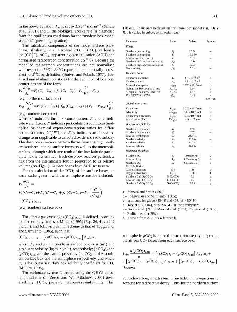
Table 1. Input parameterisation for “baseline” model run. OnlyRns is varied in subsequent model runs.

Parameter Label Value Source

Fluxes

Northern overturning Fn 28 Sv –Southern overturning Fs 16.5 Sv –Low lat. vertical mixing fli 5 Sv –Northern high lat. vertical mixing fni 10 Sv –Southern high lat. vertical mixing fsi 10 Sv –Deep mixing fns 5 Sv –

Volumes, Areas

Total ocean volume Vo 1.3×1018m3 aTotal ocean area Ao 3.5×1014m2 aMass of atmosphere Vatm 1.773×1020mol bN. high lat. box area/Total area An/Ao 0.07 cS. high lat. box area/Total area As /Ao 0.17 cVol. NDW/Vol. SDW Rns 1.43 a

(see text)

Global inventories

Phosphate Pglob 2.769×1015mol bAlkalinity Alk glob 3.12×1018mol dTotal carbon inventory Cglob 3.03×1018mol dRadiocarbon (14C) 14Cglob 3.01×106 mol d

Temperature, Salinity

Northern temperature Tn 5◦C –Southern temperature Ts 1◦C –Low lat. temperature Tl 21.5◦C –Northern salinity Sm 35.0‰ –Southern salinity Ss 34.7‰ –Low lat. salinity Sl 36.0‰ –

Restoring phosphate

Southern PO4 Ps 1.9µmol kg−1 eLow lat. PO4 Pl 0.2µmol kg−1 eNorthern PO4 Pn 0.5µmol kg−1 eRedfield RatiosCarbon/phosphate C/P 130 bOxygen/phosphate O2/P 138 fSouthern CaCO3/TCO2 S- Ca/CO2 0.2 gLow lat. CaCO3/TCO2 L- Ca/CO2 0.2 gNorthern CaCO3/TCO2 N- Ca/CO2 0.25 g

a – Menard and Smith (1966);b – Toggweiler and Sarmiento (1985);c – estimates for globe>50◦ S and 40% of>50◦ N;d – Key et al. (2004), plus 596 Gt C in the atmosphere;e – Garcia et al. (2006), Marchal et al. (1998); Najjar et al. (1992);f – Redfield et al. (1962);g – derived from Alk/P in reference b.

atmosphericpCO2 is updated at each time step by integratingthe air-sea CO2 fluxes from each surface box:

Vatmd(pCO2)atm

dt=[(pCO2)s − (pCO2)atm

]Asgsαs+

+[(pCO2)l − (pCO2)atm

]Alglαl +

[(pCO2)n − (pCO2)atm

]Angnαn

For radiocarbon, an extra term is included in the equations toaccount for radioactive decay. Thus for the northern surface



box, the mass balance equation for radiocarbon is:

Vn

dCn

dt= Fn(Cl − Cn) + fni(Ci − Cn) − Pn

C∗

P ∗+

FAO − λCn

Hereλ is the radiocarbon decay constant (1.2097 e−4 yr−1).Radiocarbon is transported as a concentration (µmol kg−1),such that the ratio of radiocarbon to total carbon (R14C) isdetermined by dividing the radiocarbon concentration by thetotal carbon concentration of the relevant box at each time-step. The normalised radiocarbon concentration is then de-termined as:

114Cbox =

(R14Cbox

R14Cstd− 1

)×1000

The radiocarbon concentrations of the various boxes are ex-pressed relative to the pre-industrial standard14C/C ratio of1.176 e−12. Biological uptake/release of radiocarbon andcosmogenic radiocarbon production are not treated explic-itly in this model. Instead these terms are diagnosed for anequilibrium atmospheric radiocarbon concentration equal tothe pre-industrial standard (14C/C=1.176 e−12). Once diag-nosed, both terms are kept constant for experiments that in-volve modifications in box-model geometry. The global ra-diocarbon inventory is also fixed at its pre-industrial value,and can be maintained at this constant level once a pre-industrial equilibrium has been attained. Atmosphere –ocean exchange of radiocarbon is calculated as formulatedfor example by (Muller et al., 2006), such that:

FAO = gAoKh

pCO2−atm

TCO2−o

(R14Catm − R14Co

)whereFAO is the atmosphere to ocean radiocarbon flux,g

is the gas piston velocity (fixed at 3 ms−1), Ao is the ex-posed ocean box area,Kh is the CO2 solubility constantfor the ocean surface and subscripts−atm and −o refer toatmospheric- and oceanic carbon concentrations or radiocar-bon ratios.

A numerical integration method (ODE-45 in Matlab’sSimulink) is used to update the box concentration at the endof each time step, until all boxes reach a steady equilibrium.In order for radiocarbon to reach equilibrium the model mustbe integrated for∼20 000 model years. In the model, a cor-rection scheme is used to check that the global inventoriesof phosphate, alkalinity and (radio-) carbon do not drift, andare all maintained at prescribed constant values. This cor-rection scheme in fact only needs to be invoked for radio-carbon, since it is the only modelled species that includesdiagnosed net input/output terms (production, decay and ter-restrial biosphere uptake). Radiocarbon inventory correctionfactors thus differ from 1 during the “wind-up” to equilib-rium, while the atmospheric input and output terms (cosmo-genic production minus biosphere uptake) are being diag-nosed. Note that box-volumes in the model do not change

during simulations (dV/dt=0). It should also be noted thatalthough the flow scheme of the box model essentially rep-resents an Atlantic Ocean (i.e. it has two deep overturning“limbs”), it is scaled to global proportions so that the vol-umes and concentrations of the atmosphere and the oceanbalance with global inventories (all of which are fixed in-put parameters). Nevertheless, the volumes of the two deep-water boxes are scaled relative to each other according to thehypothesised representation of North Atlantic and Antarcticdeep-water end-members throughout the global ocean.

The model is initiated with the concentrations of all boxesset to the global average, except for thepCO2 of the surfaceboxes and the atmosphere, which are set arbitrarily close tozero (this avoids singularities in the calculation of initial ra-diocarbon concentrations). Equilibrium outcomes were notfound to be sensitive to changes in these initial concentra-tion conditions, since global inventories are maintained. Inall model runs temperatures and salinities are also kept con-stant, in order to investigate exclusively the effect of water-mass geometry changes.

3.1 Model parameterisation and sensitivity

The parameterisation of the model’s mass transport and mix-ing rate terms is outlined in Table 1. Circulation rates forthe (modern) northern and southern overturning loops wereinitially set according to (Ganachaud and Wunsch, 2000).These export rates were then augmented in fixed proportionto each other (1:1.7) in order to achieve deep ocean radio-carbon concentrations that more closely matched the mod-ern ocean (average deep-ocean age∼1400 years) and suchthat atmospheric carbon dioxide reached an appropriate pre-industrial value (∼ 280 ppm) when restoring to modern sur-face phosphate concentration estimates (see below). Mixingrates between boxes were set arbitrarily to 10 Sv in the highlatitudes and 5 Sv for the deep-ocean and the low-latitudesurface ocean, where it can be argued that up-welling shouldbe small compared to high-latitude overturning (Gnanade-sikan et al., 2007). The sensitivity of the variable biologi-cal export was diagnosed by restoring to prescribed surfacephosphate concentrations, as described above, once appropri-ate mass transport rates were estimated (see Table 1). Withthe net biological export to the deep boxes estimated to be∼10% of export production at 100 m (Martin et al., 1987),the total biological export at 100 m in the baseline model runis ∼20 PgC yr−1. Although this value is rather high, there isample scope for reducing it by prescribing a more sluggishnet overturning rate in the model, while maintaining approx-imate pre-industrial atmosphericpCO2, and re-diagnosing(necessarily lower) biological uptake rates. As illustrated be-low, this can be done without significantly affecting the car-bon and radiocarbon distributions in the model, and indeedwithout affecting the outcome of this study. Directly tuningthe model to expected net biological export rates (closer to



∼10 PgC yr−1, Kohler et al., 2005) can therefore be safelyavoided.

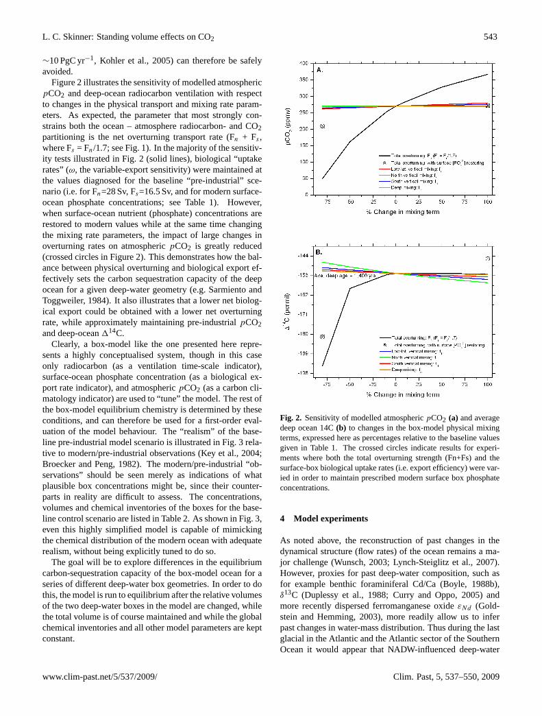
Figure 2 illustrates the sensitivity of modelled atmosphericpCO2 and deep-ocean radiocarbon ventilation with respectto changes in the physical transport and mixing rate param-eters. As expected, the parameter that most strongly con-strains both the ocean – atmosphere radiocarbon- and CO2partitioning is the net overturning transport rate (Fn + Fs ,where Fs = Fn/1.7; see Fig. 1). In the majority of the sensitiv-ity tests illustrated in Fig. 2 (solid lines), biological “uptakerates” (ω, the variable-export sensitivity) were maintained atthe values diagnosed for the baseline “pre-industrial” sce-nario (i.e. for Fn=28 Sv, Fs=16.5 Sv, and for modern surface-ocean phosphate concentrations; see Table 1). However,when surface-ocean nutrient (phosphate) concentrations arerestored to modern values while at the same time changingthe mixing rate parameters, the impact of large changes inoverturning rates on atmosphericpCO2 is greatly reduced(crossed circles in Figure 2). This demonstrates how the bal-ance between physical overturning and biological export ef-fectively sets the carbon sequestration capacity of the deepocean for a given deep-water geometry (e.g. Sarmiento andToggweiler, 1984). It also illustrates that a lower net biolog-ical export could be obtained with a lower net overturningrate, while approximately maintaining pre-industrialpCO2and deep-ocean114C.

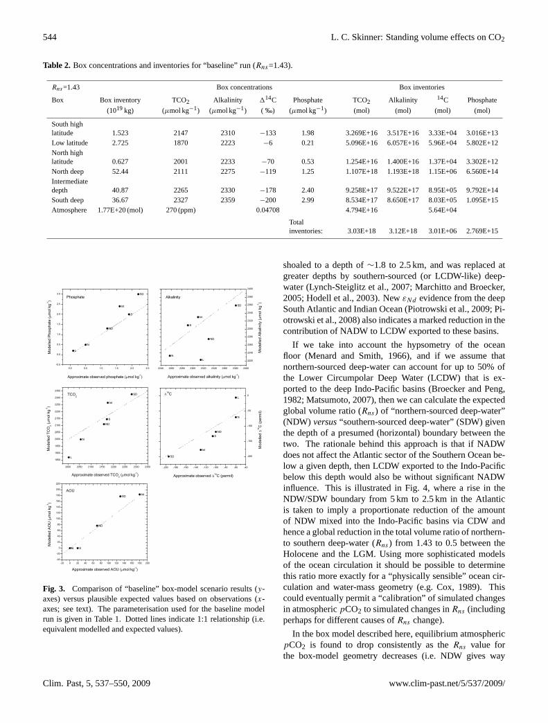
Clearly, a box-model like the one presented here repre-sents a highly conceptualised system, though in this caseonly radiocarbon (as a ventilation time-scale indicator),surface-ocean phosphate concentration (as a biological ex-port rate indicator), and atmosphericpCO2 (as a carbon cli-matology indicator) are used to “tune” the model. The rest ofthe box-model equilibrium chemistry is determined by theseconditions, and can therefore be used for a first-order eval-uation of the model behaviour. The “realism” of the base-line pre-industrial model scenario is illustrated in Fig. 3 rela-tive to modern/pre-industrial observations (Key et al., 2004;Broecker and Peng, 1982). The modern/pre-industrial “ob-servations” should be seen merely as indications of whatplausible box concentrations might be, since their counter-parts in reality are difficult to assess. The concentrations,volumes and chemical inventories of the boxes for the base-line control scenario are listed in Table 2. As shown in Fig. 3,even this highly simplified model is capable of mimickingthe chemical distribution of the modern ocean with adequaterealism, without being explicitly tuned to do so.

The goal will be to explore differences in the equilibriumcarbon-sequestration capacity of the box-model ocean for aseries of different deep-water box geometries. In order to dothis, the model is run to equilibrium after the relative volumesof the two deep-water boxes in the model are changed, whilethe total volume is of course maintained and while the globalchemical inventories and all other model parameters are keptconstant.


24

Figure 2

Figure 2. Sensitivity of modelled atmospheric pCO2 (A) and average deep ocean ∆14C (B) to changes in the

box-model physical mixing terms, expressed here as percentages relative to the baseline values given in Table 1. The crossed circles indicate results for experiments where both the total overturning strength (Fn+Fs) and the surface-box biological uptake rates (i.e. export efficiency) were varied in order to maintain prescribed

modern surface box phosphate concentrations.

Fig. 2. Sensitivity of modelled atmosphericpCO2 (a) and averagedeep ocean 14C(b) to changes in the box-model physical mixingterms, expressed here as percentages relative to the baseline valuesgiven in Table 1. The crossed circles indicate results for experi-ments where both the total overturning strength (Fn+Fs) and thesurface-box biological uptake rates (i.e. export efficiency) were var-ied in order to maintain prescribed modern surface box phosphateconcentrations.

4 Model experiments

As noted above, the reconstruction of past changes in thedynamical structure (flow rates) of the ocean remains a ma-jor challenge (Wunsch, 2003; Lynch-Steiglitz et al., 2007).However, proxies for past deep-water composition, such asfor example benthic foraminiferal Cd/Ca (Boyle, 1988b),δ13C (Duplessy et al., 1988; Curry and Oppo, 2005) andmore recently dispersed ferromanganese oxideεNd (Gold-stein and Hemming, 2003), more readily allow us to inferpast changes in water-mass distribution. Thus during the lastglacial in the Atlantic and the Atlantic sector of the SouthernOcean it would appear that NADW-influenced deep-water



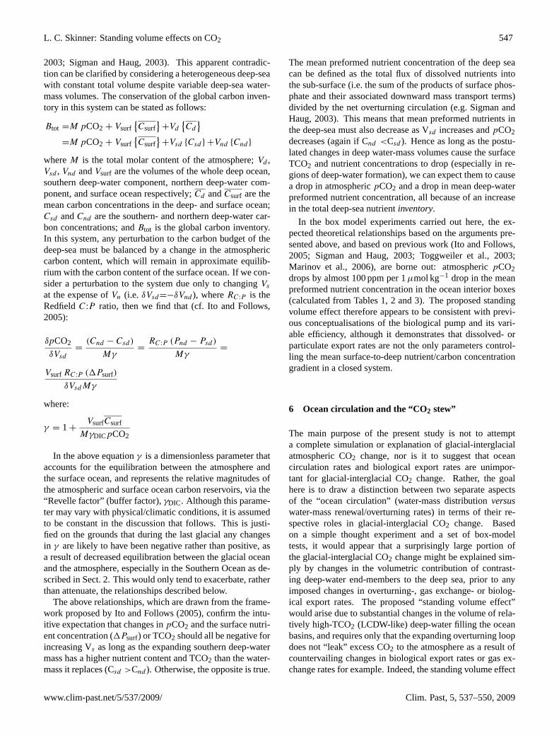
Table 2. Box concentrations and inventories for “baseline” run (Rns=1.43).

Rns=1.43 Box concentrations Box inventories

Box Box inventory TCO2 Alkalinity 114C Phosphate TCO2 Alkalinity 14C Phosphate

(1019kg) (µmol kg−1) (µmol kg−1) ( ‰) (µmol kg−1) (mol) (mol) (mol) (mol)

South highlatitude 1.523 2147 2310 −133 1.98 3.269E+16 3.517E+16 3.33E+04 3.016E+13Low latitude 2.725 1870 2223 −6 0.21 5.096E+16 6.057E+16 5.96E+04 5.802E+12North highlatitude 0.627 2001 2233 −70 0.53 1.254E+16 1.400E+16 1.37E+04 3.302E+12North deep 52.44 2111 2275 −119 1.25 1.107E+18 1.193E+18 1.15E+06 6.560E+14Intermediatedepth 40.87 2265 2330 −178 2.40 9.258E+17 9.522E+17 8.95E+05 9.792E+14South deep 36.67 2327 2359 −200 2.99 8.534E+17 8.650E+17 8.03E+05 1.095E+15Atmosphere 1.77E+20 (mol) 270 (ppm) 0.04708 4.794E+16 5.64E+04

Totalinventories: 3.03E+18 3.12E+18 3.01E+06 2.769E+15

Fig. 3. Comparison of “baseline” box-model scenario results (y-axes) versus plausible expected values based on observations (x-axes; see text). The parameterisation used for the baseline modelrun is given in Table 1. Dotted lines indicate 1:1 relationship (i.e.equivalent modelled and expected values).

shoaled to a depth of∼1.8 to 2.5 km, and was replaced atgreater depths by southern-sourced (or LCDW-like) deep-water (Lynch-Steiglitz et al., 2007; Marchitto and Broecker,2005; Hodell et al., 2003). NewεNd evidence from the deepSouth Atlantic and Indian Ocean (Piotrowski et al., 2009; Pi-otrowski et al., 2008) also indicates a marked reduction in thecontribution of NADW to LCDW exported to these basins.

If we take into account the hypsometry of the oceanfloor (Menard and Smith, 1966), and if we assume thatnorthern-sourced deep-water can account for up to 50% ofthe Lower Circumpolar Deep Water (LCDW) that is ex-ported to the deep Indo-Pacific basins (Broecker and Peng,1982; Matsumoto, 2007), then we can calculate the expectedglobal volume ratio (Rns) of “northern-sourced deep-water”(NDW) versus“southern-sourced deep-water” (SDW) giventhe depth of a presumed (horizontal) boundary between thetwo. The rationale behind this approach is that if NADWdoes not affect the Atlantic sector of the Southern Ocean be-low a given depth, then LCDW exported to the Indo-Pacificbelow this depth would also be without significant NADWinfluence. This is illustrated in Fig. 4, where a rise in theNDW/SDW boundary from 5 km to 2.5 km in the Atlanticis taken to imply a proportionate reduction of the amountof NDW mixed into the Indo-Pacific basins via CDW andhence a global reduction in the total volume ratio of northern-to southern deep-water (Rns) from 1.43 to 0.5 between theHolocene and the LGM. Using more sophisticated modelsof the ocean circulation it should be possible to determinethis ratio more exactly for a “physically sensible” ocean cir-culation and water-mass geometry (e.g. Cox, 1989). Thiscould eventually permit a “calibration” of simulated changesin atmosphericpCO2 to simulated changes inRns (includingperhaps for different causes ofRns change).

In the box model described here, equilibrium atmosphericpCO2 is found to drop consistently as theRns value forthe box-model geometry decreases (i.e. NDW gives way




26

Figure 4.

Figure 4. Illustration of how the volume ratio (Rns) of ‘northern’ (NDW) to ‘southern’ (SDW) water-masses is hypothesised to change based on water-mass boundary shoaling and given the hypsometry of the sea floor. The left hand panel shows changing water-mass ratio Rns versus the water depth of a presumed horizontal

water-mass boundary. Solid dots indicate estimated values for ‘modern’ and last glacial maximum (LGM) hydrography. The right hand panel shows how the sea floor area varies with water depth in the Atlantic and Indo-Pacific basins. Shading illustrates how Rns is calculated, by assuming that SDW fills the abyssal ocean up to the presumed water-mass boundary, while NDW fills only half of the Indo-Pacific basin and all of the

Atlantic basin above this. The volume ratio Rns for a given fill depth is thus estimated as the volume above the fill depth in the Atlantic, plus half the volume above the fill depth in the Indo-Pacific, divided by the volume below the fill depth in the Atlantic and the Indo-Pacific plus half the volume above the fill depth in the Indo-Pacific. This tempers the exaggeration in volume change that would otherwise result from treating the whole

ocean as analogous to the Atlantic.

Fig. 4. Illustration of how the volume ratio (Rns ) of “north-ern” (NDW) to “southern” (SDW) water-masses is hypothesisedto change based on water-mass boundary shoaling and given thehypsometry of the sea floor. The left hand panel shows changingwater-mass ratioRns versus the water depth of a presumed horizon-tal water-mass boundary. Solid dots indicate estimated values for“modern” and last glacial maximum (LGM) hydrography. The righthand panel shows how the sea floor area varies with water depth inthe Atlantic and Indo-Pacific basins. Shading illustrates howRns

is calculated, by assuming that SDW fills the abyssal ocean up tothe presumed water-mass boundary, while NDW fills only half ofthe Indo-Pacific basin and all of the Atlantic basin above this. Thevolume ratioRns for a given fill depth is thus estimated as the vol-ume above the fill depth in the Atlantic, plus half the volume abovethe fill depth in the Indo-Pacific, divided by the volume below thefill depth in the Atlantic and the Indo-Pacific plus half the volumeabove the fill depth in the Indo-Pacific. This tempers the exaggera-tion in volume change that would otherwise result from treating thewhole ocean as analogous to the Atlantic.

to SDW). This is shown in Fig. 5, where a shift in theNDW/SDW water-mass boundary from 5 km to 2.5 km (ora change inRns from 1.43 to 0.5) corresponds to a dropin equilibrium atmosphericpCO2 of just over 25 ppm. Thebox model volumes and chemical inventories for the hypoth-esised “glacial” water-mass geometry (2.5 km NDW/SDWwater-mass boundary,Rns=0.5) are summarised in Table 3.As expected, a “standing volume effect” such as describedhere is not going to account for the entirety of glacial-interglacialpCO2 change. However, the important and per-haps surprising observation is that this mechanism might ac-count for nearly as much of the glacial-interglacial atmo-sphericpCO2 change as has been attributed to other fun-damental mechanisms, such as sea-surface cooling, carbon-ate compensation, or ocean fertilisation (Sigman and Boyle,2000; Peacock et al., 2006; Brovkin et al., 2007).


27

Figure 5

Figure 5. Sensitivity of modelled atmospheric pCO2 to changes in the NDW/SDW volume ratio (Rns). As the water-mass boundary shoals from ~5km (modern baseline) to ~ 2.5km (last glacial), Rns is estimated to change

from 1.43 to 0.5. This results in a 26ppm drop in atmospheric pCO2 in the box model.

Fig. 5. Sensitivity of modelled atmospheric pCO2 to changes inthe NDW/SDW volume ratio (Rns ). As the water-mass boundaryshoals from 5 km (modern baseline) to 2.5 km (last glacial),Rns

is estimated to change from 1.43 to 0.5. This results in a 26 ppmdrop in atmosphericpCO2 in the box model.

5 Discussion: sustaining a “standing volume” effect

The box model experiments illustrated in Fig. 5 appearto confirm the thought experiment described in Sect. 2.0,whereby an ocean that is dominated by LCDW-like deep wa-ter holds more CO2. In order to operate effectively however,this sequestration mechanism requires three conditions: 1)there must be rather large changes in water-mass volumes(in the scenario envisaged here∼60% of the Atlantic and∼30% of the Indo-Pacific is affected by the reduced NADWcontribution); 2) the expanding water-mass must have highTCO2 relative to the water it effectively displaces; and 3) theexpanding southern overturning loop must not “leak” CO2to the atmosphere very efficiently. These three conditionsstem from the fact that the standing volume effect operatesby causing an increase in the “efficiency” of the biologicalpump (via an increase in the deep sea nutrient pool), and byenhancing the solubility pump (via an expansion of a water-mass that is colder and relatively poorly equilibrated withthe atmosphere), in both cases for a given overturning fluxand polar outcrop area. If combined with a lower globalaverage temperature, the expansion of a colder deep water-mass would further reduce the average ocean heat content.Once again, the key point is that a change in deep water-massgeometry could provide an effective means of keeping theocean interior cold (against diffusive and geothermal warm-ing from above and below), without any changes in overalloverturning rates. This could be particularly important forenhancing the vertical abyssal temperature gradient if indeedthe advection rate of cold deep-water from the poles was sig-nificantly reduced during the last glacial, relative to today.



Table 3. Box concentrations and inventories for “glacial” run (Rns=0.5).

Rns=1.43 Box inventories Box inventories

Box Box inventory TCO2 Alkalinity 114C Phosphate TCO2 Alkalinity 14C Phosphate

(1019kg) (µmol kg−1) (µmol kg−1) (‰) (µmol kg−1) (mol) (mol) (mol) (mol)

South highlatitude 1.523 2114 2293 −119 1.60 3.220E+16 3.493E+16 3.34E+04 2.437E+13Low latitude 2.725 1842 2213 11 0.00 5.019E+16 6.030E+16 5.97E+04 0.000E+00North highlatitude 0.627 1967 2222 −53 0.30 1.234E+16 1.393E+16 1.37E+04 1.881E+12North deep 29.7 2071 2261 −100 1.00 6.150E+17 6.715E+17 6.51E+05 2.970E+14Intermediatedepth 40.87 2224 2314 −162 2.10 9.087E+17 9.456E+17 8.96E+05 8.583E+14South deep 59.4 2303 2346 −190 2.70 1.368E+18 1.394E+18 1.30E+06 1.604E+15Atmosphere 1.77E+20 (mol) 244 (ppm) 20.02 4.333E+16 5.20E+04

Totalinventories: 3.03E+18 3.12E+18 3.01E+06 2.769E+15

Because the proposed standing volume effect operatesvia modulations of the biological and solubility pumps, itshould combine additively with other imposed changes ingas-exchange or nutrient utilisation in the Southern Ocean,due to sea-ice expansion, increased upper-ocean stratificationor ocean fertilisation for example. This is shown in Fig. 6,which shows that independently imposed changes in South-ern Ocean air-sea gas exchange do not attenuate the standingvolume effect at all, while a completely depleted SouthernOcean nutrient pool only attenuates the standing volume ef-fect by∼50% (due to the near elimination of the surface nu-trient pool that the expanding SDW can draw from). Oneimplication of the results shown in Fig. 6 is that imposedchanges in gas exchange or biological export will result ina greater change in atmosphericpCO2 if they are accompa-nied by an increase in the volumetric dominance of southern-sourced deep-water.

Previously, it has been suggested on the basis of first or-der principles and numerical modelling experiments that ifglobal nutrient inventories are maintained while surface nu-trients are depleted, either via reduced overturning rates orincreased biological export rates, atmosphericpCO2 willvary in proportion to the resulting average preformed nutri-ent concentration of the deep sea (Ito and Follows, 2005;Sigman and Haug, 2003; Toggweiler et al., 2003; Mari-nov et al., 2006). The average deep-sea preformed nutri-ent concentration is thus suggested to scale with atmospheicpCO2, with an estimated∼130–170 ppm change inpCO2per 1µmol kg−1 change in preformed phosphate (Ito andFollows, 2005; Sigman and Haug, 2003; Marinov et al.,2006). One way to explain the positive correlation is that anychange that acts to reduce the mean nutrient (i.e. phosphate)concentration at the ocean surface (especially in regions ofdeepwater formation, Marinov et al., 2006) will result in:(1) a reduction of the advected nutrient flux into the ocean


28

Figure 6.

Figure 6. Sensitivity of the modelled change in atmospheric pCO2 to changes in Rns when Southern Ocean gas exchange efficiency is enhanced/reduced and Southern Ocean biological export efficiency is enhanced to

100%. The sensitivity of ∆pCO2 to Rns remains positive in each case, such that a reduction in pCO2 driven by

gas exchange or biological export change would be enhanced by a reduction in Rns.

Fig. 6. Sensitivity of the modelled change in atmosphericpCO2 tochanges inRns when Southern Ocean gas exchange efficiency is en-hanced/reduced and Southern Ocean biological export efficiency isenhanced to 100%. The sensitivity ofpCO2 toRns remains positivein each case, such that a reduction inpCO2 driven by gas exchangeor biological export change would be enhanced by a reduction inRns .

interior (thus lowering the mean preformed nutrient concen-tration of deep sea); and (2) an increase in the total nutri-ent concentration of the deep-sea (due to the conservation ofocean nutrients), thus sequestering more carbon in the deepsea.

The proposed scaling between mean deep-sea preformednutrient concentrations and atmosphericpCO2 might betaken to imply that the domination of the deep sea by LCDW-like deep water (with a relatively high preformed nutrientconcentration) would cause atmosphericpCO2 to rise, con-trary to the hypothesis presented here (Toggweiler et al.,



2003; Sigman and Haug, 2003). This apparent contradic-tion can be clarified by considering a heterogeneous deep-seawith constant total volume despite variable deep-sea water-mass volumes. The conservation of the global carbon inven-tory in this system can be stated as follows:

Btot =M pCO2 + Vsurf{Csurf

}+Vd

{Cd

}=M pCO2 + Vsurf

{Csurf

}+Vsd {Csd} +Vnd {Cnd}

whereM is the total molar content of the atmosphere;Vd ,Vsd , Vnd andVsurf are the volumes of the whole deep ocean,southern deep-water component, northern deep-water com-ponent, and surface ocean respectively;Cd andCsurf are themean carbon concentrations in the deep- and surface ocean;Csd andCnd are the southern- and northern deep-water car-bon concentrations; andBtot is the global carbon inventory.In this system, any perturbation to the carbon budget of thedeep-sea must be balanced by a change in the atmosphericcarbon content, which will remain in approximate equilib-rium with the carbon content of the surface ocean. If we con-sider a perturbation to the system due only to changingVs

at the expense ofVn (i.e. δVsd=−δVnd ), whereRC:P is theRedfieldC:P ratio, then we find that (cf. Ito and Follows,2005):

δpCO2

δVsd

=(Cnd − Csd)

Mγ=

RC:P (Pnd − Psd)

Mγ=

VsurfRC:P (1Psurf)

δVsdMγ

where:

γ = 1 +VsurfCsurf

MγDICpCO2

In the above equationγ is a dimensionless parameter thataccounts for the equilibration between the atmosphere andthe surface ocean, and represents the relative magnitudes ofthe atmospheric and surface ocean carbon reservoirs, via the“Revelle factor” (buffer factor),γDIC. Although this parame-ter may vary with physical/climatic conditions, it is assumedto be constant in the discussion that follows. This is justi-fied on the grounds that during the last glacial any changesin γ are likely to have been negative rather than positive, asa result of decreased equilibration between the glacial oceanand the atmosphere, especially in the Southern Ocean as de-scribed in Sect. 2. This would only tend to exacerbate, ratherthan attenuate, the relationships described below.

The above relationships, which are drawn from the frame-work proposed by Ito and Follows (2005), confirm the intu-itive expectation that changes inpCO2 and the surface nutri-ent concentration (1Psurf) or TCO2 should all be negative forincreasing Vs as long as the expanding southern deep-watermass has a higher nutrient content and TCO2 than the water-mass it replaces (Csd >Cnd ). Otherwise, the opposite is true.

The mean preformed nutrient concentration of the deep seacan be defined as the total flux of dissolved nutrients intothe sub-surface (i.e. the sum of the products of surface phos-phate and their associated downward mass transport terms)divided by the net overturning circulation (e.g. Sigman andHaug, 2003). This means that mean preformed nutrients inthe deep-sea must also decrease as Vsd increases andpCO2decreases (again if Cnd <Csd ). Hence as long as the postu-lated changes in deep water-mass volumes cause the surfaceTCO2 and nutrient concentrations to drop (especially in re-gions of deep-water formation), we can expect them to causea drop in atmosphericpCO2 and a drop in mean deep-waterpreformed nutrient concentration, all because of an increasein the total deep-sea nutrientinventory.

In the box model experiments carried out here, the ex-pected theoretical relationships based on the arguments pre-sented above, and based on previous work (Ito and Follows,2005; Sigman and Haug, 2003; Toggweiler et al., 2003;Marinov et al., 2006), are borne out: atmosphericpCO2drops by almost 100 ppm per 1µmol kg−1 drop in the meanpreformed nutrient concentration in the ocean interior boxes(calculated from Tables 1, 2 and 3). The proposed standingvolume effect therefore appears to be consistent with previ-ous conceptualisations of the biological pump and its vari-able efficiency, although it demonstrates that dissolved- orparticulate export rates are not the only parameters control-ling the mean surface-to-deep nutrient/carbon concentrationgradient in a closed system.

6 Ocean circulation and the “CO2 stew”

The main purpose of the present study is not to attempta complete simulation or explanation of glacial-interglacialatmospheric CO2 change, nor is it to suggest that oceancirculation rates and biological export rates are unimpor-tant for glacial-interglacial CO2 change. Rather, the goalhere is to draw a distinction between two separate aspectsof the “ocean circulation” (water-mass distributionversuswater-mass renewal/overturning rates) in terms of their re-spective roles in glacial-interglacial CO2 change. Basedon a simple thought experiment and a set of box-modeltests, it would appear that a surprisingly large portion ofthe glacial-interglacial CO2 change might be explained sim-ply by changes in the volumetric contribution of contrast-ing deep-water end-members to the deep sea, prior to anyimposed changes in overturning-, gas exchange- or biolog-ical export rates. The proposed “standing volume effect”would arise due to substantial changes in the volume of rela-tively high-TCO2 (LCDW-like) deep-water filling the oceanbasins, and requires only that the expanding overturning loopdoes not “leak” excess CO2 to the atmosphere as a result ofcountervailing changes in biological export rates or gas ex-change rates for example. Indeed, the standing volume effect



will be additive with respect to accompanying changes in bi-ological export or gas exchange around Antarctica.

Although previous studies that have simulated glacial at-mospheric CO2 using complex numerical models with ac-curate bathymetry (e.g. Heinze et al., 1991) may have al-ready included the proposed standing volume effect implic-itly, none so far have tried to identify or quantify its possi-ble impact on glacial CO2 draw-down. Although one recentexception (Brovkin et al., 2007) has suggested that the ex-pansion of AABW at the expense of NADW in the glacialocean might have caused atmospheric CO2 to drop by asmuch as 43 ppm, this estimate includes the effects of changesin deep-water overturning rates (reduced NADW export rateby ∼20% and intensified AABW export rate). The proposedstanding volume effect therefore remains to be tested ade-quately using complex numerical model simulations of theglacial ocean circulation.

If the simple standing volume mechanism proposed herefor enhancing deep-sea carbon sequestration can be incor-porated into the list of “ingredients” that have contributed toglacial-interglacial CO2 change (Peacock et al., 2006; Kohleret al., 2005; Archer et al., 2000; Sigman and Boyle, 2000), itmay help to reduce or eliminate the CO2 deficit that remainsto be explained by appealing to more equivocal or controver-sial processes. More importantly however, it may also helpus to evaluate more explicitly the role of the ‘ocean circula-tion’ as an ingredient in the glacial-interglacial “CO2 stew”,as well as the triggers that repeatedly pushed the marine car-bon cycle between glacial and interglacial modes (Paillardand Parrenin, 2004; Shackleton, 2000). This is especiallytrue if the mechanisms or timescales for changing the verticalmass transport rate in the ocean differ from those for chang-ing the (vertical) redistribution of contrasting deep-waterend-members. Indeed, a de-convolution of the expected im-pacts of an altered “ocean circulation” into renewal-rate ef-fects and standing-volume effects can only gain importanceto the extent that proxy evidence for a large reduction in thenet overturning rate of the glacial ocean remains equivocal(Lynch-Steiglitz et al., 2007), and/or theoretical support forsuch a change continues to be debated (Wunsch, 2003).

Acknowledgements.The author is grateful for helpful discussionswith E. Gloor, P. Koelher, R. Toggweiler, E. Galbraith andM. McIntyre, as well as the input of two anonymous reviewers.The author would also like to acknowledge research fellowshipsprovided by The Royal Society and Christ’s College Cambridge.

Edited by: R. Zeebe

References

Adkins, J. F., McIntyre, K., and Schrag, D. P.: The salinity, tem-perature and d18o of the glacial deep ocean, Science, 298, 1769–1773, 2002.

Archer, D. and Maier-Reimer, E.: Effect of deep-sea sedimentarycalcite preservation on atmospheric co2 concentration, Nature,367, 260–263, 1994.

Archer, D., Winguth, A., Lea, D. W., and Mahowald, N.: Whatcaused the glacial/interglacial atmosphericpco2 cycles?, Rev.Geophys., 38, 159–189, 2000.

Bard, E.: Correction of accelerator mass spectrometry 14c agesmeasured in planktonic foraminifera: Paleoceanographic impli-cations, Paleoceanography, 3, 635–645, 1988.

Barker, S., Diz, P., Vautravers, M., Pike, J., Knorr, G., Hall, I.R., and Broecker, W.: Interhemispheric atlantic seesaw responseduring the last deglaciation, Nature, 457, 1097–1102, 2009.

Boyle, E.: Cadmium and d13c paleochemical ocean distributionsduring the stage 2 glacial maximum, Ann. Rev. Earth Planet. Sci.,20, 245–287, 1992.

Boyle, E. A.: The role of vertical fractionation in controlling latequaternary atmospheric carbon dioxide, J. Geophys. Res., 93,15701–715714, 1988a.

Boyle, E. A.: Cadmium: Chemical tracer fro deepwater paleo-ceanography, Paleoceanography, 3, 471–489, 1988b.

Broecker, W. S.: Glacial to interglacial changes in ocean chemistry,Prog. Oceanogr., 11, 151–197, 1982a.

Broecker, W. S.: Ocean chemistry during glacial time, Geochim.Cosmochim. Ac., 46, 1698–1705, 1982b.

Broecker, W. S. and Peng, T. H.: Tracers in the sea, Eldigio Press,Palisades, New York, USA, 690 pp., 1982.

Broecker, W. S. and Peng, T.-H.: The cause of the glacial to inter-glacial atmospheric co2 change: A polar alkalinity hypothesis,Global Biogeochem. Cy., 3, 215–239, 1989.

Brovkin, V., Ganopolski, A., Archer, D., and Rahmstorf, S.: Low-ering glacial atmospheric co2 in response to changes in oceaniccirculation and marien biogeochemistry, Paleoceanography, 22,1–14, 2007.

Cox, M. D.: An idealized model of the world ocean. Part i: Theglobal-scale water masses, J. Phys. Oceanogr., 19, 1730–1752,1989.

Curry, W. B., Duplessy, J. C., Labeyrie, L. D., and Shackleton, N.J.: Changes in the distribution of d13c of deep water sigma-co2between the last glaciation and the holocene, Paleoceanography,3, 317–341, 1988.

Curry, W. B. and Oppo, D. W.: Glacial water mass ge-ometry and the distribution ofδ13C of sigma-CO2 inthe western atlantic ocean, Paleoceanography, 20, PA1017,doi:10.1029/2004PA001021,2005.

Denman, K. L., Brasseur, G., Chidthaisong, A., Ciasis, P., Cox, P.M., Dickinson, R. E., Hauglustaine, D., Heinze, C., Holland, E.,Jacob, D., Lohmann, U., Ramachandran, S., da Silva Dias, P.L., Wofsy, S. C., and Zhang, X.: Couplings between changesin the climate system and biogeochemistry, in: Climate change2007: The physical basis. Contribution of working group i tothe fourth assessment report of the intergovernmental panel onclimate change, edited by: Solomon, S., Qin, D., Manning, M.,Chen, Z., Marquis, M., Averyt, K. B., Tignor, M., and Miller,H. L., Cambridge University Press, Cambridge, New York, 499–587, 2007.

Dugdale, R. C.: Nutrient limitation in the sea: Dynamics, identifi-cation, and significance, Limnol. Oceanogr., 12, 685–695, 1967.

Duplessy, J.-C., Shackleton, N. J., Fairbanks, R. G., Labeyrie, L.,Oppo, D., and Kallel, N.: Deep water source variations during



the last climatic cycle and their impact on global deep water cir-culation, Paleoceanography, 3, 343–360, 1988.

Ganachaud, A. and Wunsch, C.: Improved estimates of globalocean circulation, heat transport and mixing from hydrographicdata, Nature, 408, 453–457, 2000.

Garcia, H. E., Locarnini, T. P., and Antonov, J. I.: World ocean atlas2005, volume 4, Nutrients (phosphate, nitrate, silicate), US Gov-ernment Printing Office, Washington DC, USA, 396 pp., 2006.

Gildor, H. and Tziperman, E.: Physical mechanisms behind biogeo-chemical glacial-interglacial co2variations, Geophys. Res. Lett.,28, 2421–2424, 2001.

Gnanadesikan, A., de Boer, A. M., and Mignone, B. K.: A simpletheory of the pycnocline and overturning revisited, in: Oceancirculation: Mechanisms and impacts, edited by: Schmittner, A.,Chiang, C. H., and Hemming, S. R., Geophysical monograph,AGU, Washington DC, USA, 19–32, 2007.

Goldstein, S. L. and Hemming, S. R.: Long-lived isotopic trac-ers in oceanography, paleoceanography and ice-sheet dynamics,in: Treatise on geochemistry, edited by: Elderfield, H., Elsevier,453–489, 2003.

Gordon, A. L.: Comment on the south atlantic’s role in the globalcirculation, in: The south atlantic: Present and past circulation,edited by: Wefer, G., Berger, A., Siedler, G., and Webb, D. J.,Springer-Verlag, Berlin, Heidelberg, Germany, 121–124, 1996.

Heinze, C., Maier-Reimer, E., and Winn, K.: Glacialpco2 reduc-tion by the world ocean: Experiments with the hamburg carboncycle model, Paleoceanography, 6, 395–430, 1991.

Hodell, D. A., Venz, K. A., Charles, C. D., and Ninneman, U. S.:Pleistocene vertical carbon isotope and carbonate gradients in thesouth atlantic sector of the southern ocean, Geochem. Geophys.Geosys., 4, GC1004, doi:10.1029/2002GC000367, 2003.

Ito, T. and Follows, M. J.: Preformed phosphate, soft tissue pumpand atmospheric co2, J. Mar. Res., 63, 813–839, 2005.

Keeling, R. F. and Stephens, B. B.: Antarctic sea ice and the controlof pleistocene climate instability, Paleoceanography, 16, 112–131, 2001.

Keigwin, L. D. and Lehmann, S. J.: Deep circulation change linkedto heinrich event 1 and younger dryas in a mid-depth north at-lantic core, Paleoceanography, 9, 185–194, 1994.

Keigwin, L. D.: Radiocarbon and stable isotope constraints on lastglacial maximum and younger dryas ventilation in the westernnorth atlantic, Paleoceanography, 19, 1–15, 2004.

Key, R. M., Kozyr, A., Sabine, C., Lee, K., Wanninkhof, R., Bullis-ter, J. L., Feely, R. A., Millero, F. J., Mordy, C., and Peng, T.-H.:A global ocean carbon climatology: Results from the global dataanalysis project (glodap), Global Biogeochem. Cycles, 18, 1–23,2004.

Kim, S.-J., Flato, G. M., and Boer, G. J.: A coupled climate modelsimulation of the last glacial maximum, part 2: Approach to equi-librium, Clim. Dynam., 20, 635–661, 2003.

Knox, F. and McElroy, M.: Changes in atmospheric co2: Influenceof marine biota at high latitude, J. Geophys. Res., 89, 4629–4637,1984.

Kohler, P., Fischer, H., Munhoven, G., and Zeebe, R. E.: Quanti-tative interpretation of atmospheric carbon records over the lastglacial termination, Global Biogeochem. Cy., 19, 1–24, 2005.

Lynch-Steiglitz, J., Adkins, J. F., Curry, W. B., Dokken, T., Hall, I.R., Heguera, J. C., Hirschi, J. J.-M., Ivanova, E. V., Kissel, C.,Marchal, O., Marchitto, T. M., McCave, I. N., McManus, J. F.,

Mulitza, S., Ninneman, U. S., Peeters, F. J. C., Yu, E.-F., andZahn, R.: Atlantic meridional overturning circulation during thelast glacial maximum, Science, 316, 66–69, 2007.

Marchal, O., Stocker, T. F., and Joos, F.: A latitude-depth,circulation-biochemical ocean model for paleoclimate studies.Development and sensitivities, Tellus, 50B, 290–316, 1998.

Marchal, O. and Curry, W. B.: On the abyssal circulation in theglacial atlantic, J. Phys. Oceanogr., 38, 2014–2037, 2008.

Marchitto, T. M., Oppo, D. W., and Curry, W. B.: Paired benthicforaminiferal cd/ca and zn/ca evidence for a greatly increasedpresence of southern ocean water in the glacial north atlantic,Paleoceanography, 17, 10.11–10.16, 2002.

Marchitto, T. M. and Broecker, W.: Deep water mass geometry inthe glacial atlantic ocean: A review of constraints from the pa-leonutrient proxy cd/ca, Geochem. Geophys. Geosys., 7, 1–16,2005.

Marchitto, T. M., Lehman, S. J., Otiz, J. D., Fluckiger, J., and vanGeen, A.: Marine radiocarbon evidence for the mechanism ofdeglacial atmospheric co2 rise, Science, 316, 1456–1459, 2007.

Marinov, I., Gnadesikan, A., Toggweiler, J. R., and Sarmiento, J. L.:The southern ocean biogeochemical divide, Nature, 441, 964–967, 2006.

Martin, J. H., Knauer, G. A., Karl, D. M., and Broenkow, W. W.:Vertex: Carbon cycling in the northeast pacific, Deep-Sea Res.,34, 267–286, 1987.

Matsumoto, K.: Radiocarbon-based circulation age of the worldoceans, J. Geophys. Res., 112, 1–7, 2007.

Menard, H. W. and Smith, S. M.: Hypsometry of ocean basinprovinces, J. Geophys. Res., 71, 4305–4325, 1966.

Michel, E., Labeyrie, L., Duplessy, J.-C., and Gorfti, N.: Coulddeep subantarctic convection feed the worl deep basins duringlast glacial maximum?, Paleoceanography, 10, 927–942, 1995.

Millero, F. J.: Thermodynamics of the carbon dioxide system in theoceans, Geochim. Cosmochim. Ac., 59, 661–677, 1995.

Muller, S. A., Joos, F., Edwards, N. R., and Stocker, T. F.: Watermass distribution and ventilation time scales in a cost-efficient,three-dimensional ocena model, J. Climate, 19, 5479–5499,2006.

Najjar, R. G., Sarmiento, J. L., and Toggweiler, J. R.: Downwardtransport and fate of organic matter in the ocean: Simulationswith a general circulation model, Global Biogeochem. Cy. , 6,45–76, 1992.

Naviera Garabato, A. C., Polzin, K. L., King, B. A., Heywood, K.J., and Visbeck, M.: Widespread intense turbulent mixing in thesouthern ocean, Science, 303, 210–213, 2004.

Ninneman, U. S. and Charles, C. D.: Changes in the mode ofsouthern ocean circulation over the last glacial cycle revealed byforaminiferal stable isotopic variability, Earth Planet. Sci. Lett.,201, 383–396, 2002.

Oppo, D. and Fairbanks, R. G.: Atlantic ocean thermohaline cir-culation of the last 150 000 years: Relationship to climate andatmospheric co2, Paleoceanography, 5, 277–288, 1990.

Oppo, D. W., Fairbanks, R. G., Gordon, A. L., and Shackleton,N. J.: Late pleistocene southern ocean d13c variability, Paleo-ceanography, 5, 43–54, 1990.

Orsi, A. H., Johnson, G. C., and Bullister, J. L.: Circulation, mixingand production of antarctic bottom water, Prog. Oceanogr., 43,55–109, 1999.

Paillard, D. and Parrenin, F.: The antarctic ice sheet and the trig-



gering of deglaciations, Earth Planet. Sci. Lett., 227, 263–271,2004.

Peacock, S., Lane, E., and Restrepo, M.: A possible sequence ofevents for the generalized glacial-interglacial cycle, Global Bio-geochem. Cy., 20, 1–17, 2006.

Piotrowski, A., Goldstein, S. L., Hemming, S. R., and Fairbanks, R.G.: Temporal relationships of carbon cycling and ocean circula-tion at glacial boundaries, Science, 307, 1933–1938, 2005.

Piotrowski, A. M., Goldstein, S. L., Hemming, S. R., and Fairbanks,R. G.: Intensification and variability of ocean thermohaline cir-culation through the last deglaciation, Earth Planet. Sci. Lett.,225, 205–220, 2004.

Piotrowski, A. M., Goldstein, S. L., Hemming, S. R., Fairbanks,R. G., and Zylberberg, D. R.: Oscillating glacial northern andsouthern deep water formation from combined neodymium andcarbon isotopes, Earth Planet. Sci. Lett., 272, 394–405, 2008.

Piotrowski, A. M., Banakar, V. K., Scrivner, A., Elderfield, H., Galy,A., and Dennis, A.: Indian ocean circulation and productivityduring hte last glacial cycle, Earth Planet. Sci. Lett., 285, 179–189, 2009.

Redfield, A. C., Ketchum, B. H., and Richards, F. A.: The influenceof organisms on the composition of sea water, in: The sea, editedby: Hill, M. N., Wiley-Interscience, New York, USA, 26–77,1962.

Robinson, L. F., Adkins, J. F., Keigwin, L. D., Southon, J., Fernan-dez, D. P., Wang, S.-L., and Scheirer, D. S.: Radiocarbon vari-ability in the western north atlantic during the last deglaciation,Science, 310, 1469–1473, 2005.

Rutberg, R. L., Heming, S. R., and Goldstein, S. L.: Reduced northatlantic deep water flux to the glacial southern ocean inferredfrom neodymium isotope ratios, Nature, 405, 935–938, 2000.

Sabine, C., Feely, R. A., Gruber, N., Key, R. M., Lee, K., Bullister,J. L., Wanninkhof, R., Wong, C. S., Wallace, D. W. R., Tilbrook,B., Millero, F. J., Peng, T.-H., Kozyr, A., Ono, T., and Rios, A. F.:The oceanic sink for anthropogenic co2, Science, 305, 367–371,2004.

Sarmiento, J. L. and Toggweiler, R.: A new model for the role of theoceans in determining atmosphericpco2, Nature, 308, 621–624,1984.

Schulz, M., Seidov, D., Sarnthein, M., and Stattegger, K.: Mod-eling ocean-atmosphere carbon budgets during the last glacialmaximum-heinrich 1 meltwater event-bolling transition, Int. J.Earth Sci. (Geol Rundsch), 90, 412–425, 2001.

Shackleton, N. J.: The 100,000-year ice-age cycle identified andfound to lag temperature, carbon dioxide and orbital eccentric-ity., Science, 289, 1897–1902, 2000.

Shin, S. I., Liu, Z., Otto-Bliesner, B. L., Brady, E. C., Kutzbach,J. E., and Harrison, S. P.: A simulation of the last glacial max-imumclimate using the ncar-ccsm, Clim. Dynam., 20, 127–151,2003.

Siegenthaler, U. and Wenk, T.: Rapid atmospheric co2 variationsand ocean circulation, Nature, 308, 624–625, 1984.

Siegenthaler, U., Stocker, T. F., Monnin, E., Luthi, D., Schwan-der, J., Stauffer, B., Raynaud, D., Barnola, J.-M., Fischer, H.,Masson-Delmotte, V., and Jouzel, J.: Stable carbon cycle -climate relationship during the late pleistocene, Science, 310,1313–1317, 2005.

Sigman, D. M. and Boyle, E. A.: Glacial/interglacial variations inatmospheric carbon dioxide, Nature, 407, 859–869, 2000.

Sigman, D. M. and Haug, G. H.: The biological pump in the past,in: Treatise on geochemistry, edited by: Elderfield, H., Elsevier,491–528, 2003.

Skinner, L. C. and Shackleton, N. J.: Rapid transient changes innortheast atlantic deep-water ventilation-age across terminationi, Paleoceanography, 19, 1–11, 2004.

Sloyan, B. and Rintoul, S. R.: The southern limb of the global over-turning circulation, J. Phys. Oceanogr., 31, 143–173, 2001.

Speer, K., Rintoul, S. R., and Sloyan, B.: The diabatic deacon cell,J. Phys. Oceanogr., 30, 3212–3222, 2000.

Stuiver, M. and Polach, H. A.: Reporting of 14C data, Radiocarbon,19, 355–363, 1977.

Toggweiler, J. R., and Sarmiento, J. L.: Glacial to interglacialchanges in atmospheric carbon dioxide: The critical role of oceansurface water in high latitudes, in: The carbon cycle and atmo-spheric co2: Natural variations archean to present, Geophysicalmonograph, American Geophysical Union, 163–184, 1985.

Toggweiler, J. R.: Variation of atmospheric co2 by ventilation of theocean’s deepest water, Paleoceanography, 14, 571–588, 1999.

Toggweiler, J. R., Murnane, R., Carson, S., Gnanadesikan, A., andSarmiento, J. L.: Representation of the carbon cycle in box mod-els and gcms: 2. Organic pump, Global Biogeochem. Cy., 17,27.21–27.13, 2003.

Tziperman, E. and Gildor, H.: On the mid-pleistocene transitionto 100-kyr glacial cycles and the asymmetry between glacia-tion and deglaciation times, Paleoceanography, 18, PA1001,doi:10.1029/2001PA000627, 2003.

Watson, A. J. and Naveira Garabato, A. C.: The role of southernocean mixing and upwelling in glacial-interglacial atmosphericco2 change, Tellus, 58B, 73–87, 2006.

Webb, D. J. and Suginohara, N.: Vertical mixing in the ocean, Na-ture, 409, 37 pp., 2001, 2001.

Wunsch, C.: Determining paleoceanographic circulations, with em-phasis on the last glacial maximum, Quat. Sci. Rev., 22, 371–385, 2003.

Yu, J. and Elderfield, H.: Benthic foraminiferal b/ca ratios reflectdeep water carbonate saturation state, Earth Planet. Sci. Lett.,258, 73–86, 2007.

Zeebe, R. E. and Wolf-Gladrow, D.: Co2 in seawater: Equilibrium,kinetics, isotopes, Elsevier oceanography series, Elsevier, Ams-terdam NL, 2001.


glacial-interglacial atmospheric co2 change: a possible “standing

Documents