oracle® crystal ball decision optimizer · oracle® crystal ball decision optimizer oracle®...
TRANSCRIPT

Oracle® Crystal Ball Decision OptimizerOracle® Crystal Ball Suite
OptQuest User's Guide
Release 11.1.2.4.850
Crystal Ball Decision Optimizer OptQuest User's Guide, 11.1.2.4.850
Copyright © 1988, 2017, Oracle and/or its affiliates. All rights reserved.
Authors: EPM Information Development Team
This software and related documentation are provided under a license agreement containing restrictions on use anddisclosure and are protected by intellectual property laws. Except as expressly permitted in your license agreement orallowed by law, you may not use, copy, reproduce, translate, broadcast, modify, license, transmit, distribute, exhibit,perform, publish, or display any part, in any form, or by any means. Reverse engineering, disassembly, or decompilationof this software, unless required by law for interoperability, is prohibited.
The information contained herein is subject to change without notice and is not warranted to be error-free. If you findany errors, please report them to us in writing.
If this is software or related documentation that is delivered to the U.S. Government or anyone licensing it on behalf ofthe U.S. Government, then the following notice is applicable:
U.S. GOVERNMENT END USERS:
Oracle programs, including any operating system, integrated software, any programs installed on the hardware, and/ordocumentation, delivered to U.S. Government end users are "commercial computer software" pursuant to the applicableFederal Acquisition Regulation and agency-specific supplemental regulations. As such, use, duplication, disclosure,modification, and adaptation of the programs, including any operating system, integrated software, any programs installedon the hardware, and/or documentation, shall be subject to license terms and license restrictions applicable to the programs.No other rights are granted to the U.S. Government.
This software or hardware is developed for general use in a variety of information management applications. It is notdeveloped or intended for use in any inherently dangerous applications, including applications that may create a risk ofpersonal injury. If you use this software or hardware in dangerous applications, then you shall be responsible to take allappropriate fail-safe, backup, redundancy, and other measures to ensure its safe use. Oracle Corporation and its affiliatesdisclaim any liability for any damages caused by use of this software or hardware in dangerous applications.
Oracle and Java are registered trademarks of Oracle and/or its affiliates. Other names may be trademarks of their respectiveowners.
Intel and Intel Xeon are trademarks or registered trademarks of Intel Corporation. All SPARC trademarks are used underlicense and are trademarks or registered trademarks of SPARC International, Inc. AMD, Opteron, the AMD logo, and theAMD Opteron logo are trademarks or registered trademarks of Advanced Micro Devices. UNIX is a registered trademarkof The Open Group. Microsoft, Windows, PowerPoint, Word, Excel, Access, Office, Outlook, Visual Studio, Visual Basic,Internet Explorer, Active Directory, and SQL Server are either registered trademarks or trademarks of MicrosoftCorporation in the United States and/or other countries.
This software or hardware and documentation may provide access to or information about content, products, and servicesfrom third parties. Oracle Corporation and its affiliates are not responsible for and expressly disclaim all warranties of anykind with respect to third-party content, products, and services unless otherwise set forth in an applicable agreementbetween you and Oracle. Oracle Corporation and its affiliates will not be responsible for any loss, costs, or damages incurreddue to your access to or use of third-party content, products, or services, except as set forth in an applicable agreementbetween you and Oracle.
Contents
Documentation Accessibility . . . . . . . . . . . . . . . . . . . . . . . . . . . . . . . . . . . . . . . . . . . . . . . . . . . . . . . . . . . 7
Documentation Feedback . . . . . . . . . . . . . . . . . . . . . . . . . . . . . . . . . . . . . . . . . . . . . . . . . . . . . . . . . . . . . 9
Chapter 1. Welcome . . . . . . . . . . . . . . . . . . . . . . . . . . . . . . . . . . . . . . . . . . . . . . . . . . . . . . . . . . . . . . . . 11
Introduction . . . . . . . . . . . . . . . . . . . . . . . . . . . . . . . . . . . . . . . . . . . . . . . . . . . . . . . . . 11
How the Manual Is Organized . . . . . . . . . . . . . . . . . . . . . . . . . . . . . . . . . . . . . . . . . . . . 11
Screen Capture Notes . . . . . . . . . . . . . . . . . . . . . . . . . . . . . . . . . . . . . . . . . . . . . . . . . . 12
Getting Help . . . . . . . . . . . . . . . . . . . . . . . . . . . . . . . . . . . . . . . . . . . . . . . . . . . . . . . . . 12
Additional Resources . . . . . . . . . . . . . . . . . . . . . . . . . . . . . . . . . . . . . . . . . . . . . . . . . . 13
Chapter 2. Overview . . . . . . . . . . . . . . . . . . . . . . . . . . . . . . . . . . . . . . . . . . . . . . . . . . . . . . . . . . . . . . . . 15
Introduction . . . . . . . . . . . . . . . . . . . . . . . . . . . . . . . . . . . . . . . . . . . . . . . . . . . . . . . . . 15
What OptQuest Does . . . . . . . . . . . . . . . . . . . . . . . . . . . . . . . . . . . . . . . . . . . . . . . . . . 15
How OptQuest Works . . . . . . . . . . . . . . . . . . . . . . . . . . . . . . . . . . . . . . . . . . . . . . . . . 16
About Optimization Models . . . . . . . . . . . . . . . . . . . . . . . . . . . . . . . . . . . . . . . . . . . . . 17
Optimization Objectives . . . . . . . . . . . . . . . . . . . . . . . . . . . . . . . . . . . . . . . . . . . . . . . . 18
Forecast Statistics . . . . . . . . . . . . . . . . . . . . . . . . . . . . . . . . . . . . . . . . . . . . . . . . . . 18
Minimizing or Maximizing . . . . . . . . . . . . . . . . . . . . . . . . . . . . . . . . . . . . . . . . . . . 18
Requirements . . . . . . . . . . . . . . . . . . . . . . . . . . . . . . . . . . . . . . . . . . . . . . . . . . . . . 19
Requirement Examples . . . . . . . . . . . . . . . . . . . . . . . . . . . . . . . . . . . . . . . . . . . 19
Decision Variables . . . . . . . . . . . . . . . . . . . . . . . . . . . . . . . . . . . . . . . . . . . . . . . . . . . . 19
Constraints . . . . . . . . . . . . . . . . . . . . . . . . . . . . . . . . . . . . . . . . . . . . . . . . . . . . . . . . . . 20
Model and Solution Feasibility . . . . . . . . . . . . . . . . . . . . . . . . . . . . . . . . . . . . . . . . . . . . 21
Efficient Frontier Analysis . . . . . . . . . . . . . . . . . . . . . . . . . . . . . . . . . . . . . . . . . . . . . . . 21
Efficient Portfolios . . . . . . . . . . . . . . . . . . . . . . . . . . . . . . . . . . . . . . . . . . . . . . . . . 22
OptQuest and Process Capability . . . . . . . . . . . . . . . . . . . . . . . . . . . . . . . . . . . . . . . . . . 23
Chapter 3. Setting Up and Optimizing a Model . . . . . . . . . . . . . . . . . . . . . . . . . . . . . . . . . . . . . . . . . . . . . . 25
Introduction . . . . . . . . . . . . . . . . . . . . . . . . . . . . . . . . . . . . . . . . . . . . . . . . . . . . . . . . . 25
Overview . . . . . . . . . . . . . . . . . . . . . . . . . . . . . . . . . . . . . . . . . . . . . . . . . . . . . . . . . . . 25
For Users of OptQuest Versions Earlier Than 11.1.1.x . . . . . . . . . . . . . . . . . . . . . . . . 26
Developing a Crystal Ball Optimization Model . . . . . . . . . . . . . . . . . . . . . . . . . . . . . . . . 26
iii
Developing the Worksheet . . . . . . . . . . . . . . . . . . . . . . . . . . . . . . . . . . . . . . . . . . . . 26
Defining Assumptions, Decision Variables, and Forecasts . . . . . . . . . . . . . . . . . . . . . 27
Setting Crystal Ball Run Preferences . . . . . . . . . . . . . . . . . . . . . . . . . . . . . . . . . . . . . 27
Starting OptQuest . . . . . . . . . . . . . . . . . . . . . . . . . . . . . . . . . . . . . . . . . . . . . . . . . . . . . 28
Selecting the Forecast Objective . . . . . . . . . . . . . . . . . . . . . . . . . . . . . . . . . . . . . . . . . . 28
Selecting Decision Variables to Optimize . . . . . . . . . . . . . . . . . . . . . . . . . . . . . . . . . . . . 30
Specifying Constraints . . . . . . . . . . . . . . . . . . . . . . . . . . . . . . . . . . . . . . . . . . . . . . . . . 31
Specifying Constraints in Simple Entry Mode . . . . . . . . . . . . . . . . . . . . . . . . . . . . . . 31
Specifying Constraints in Advanced Entry Mode . . . . . . . . . . . . . . . . . . . . . . . . . . . . 31
Advanced Entry Example . . . . . . . . . . . . . . . . . . . . . . . . . . . . . . . . . . . . . . . . . 32
Constraints Editor and Related Buttons . . . . . . . . . . . . . . . . . . . . . . . . . . . . . . . . . . 33
Constraint Rules and Syntax . . . . . . . . . . . . . . . . . . . . . . . . . . . . . . . . . . . . . . . . . . 34
Constraints and Cell References in Advanced Entry Mode . . . . . . . . . . . . . . . . . . . . . 35
Constraint Types . . . . . . . . . . . . . . . . . . . . . . . . . . . . . . . . . . . . . . . . . . . . . . . . . . 36
Using Bulk Constraints . . . . . . . . . . . . . . . . . . . . . . . . . . . . . . . . . . . . . . . . . . . . . . 36
Rules for Bulk Constraints . . . . . . . . . . . . . . . . . . . . . . . . . . . . . . . . . . . . . . . . . 36
Bulk Constraints Example . . . . . . . . . . . . . . . . . . . . . . . . . . . . . . . . . . . . . . . . . 37
Setting Options . . . . . . . . . . . . . . . . . . . . . . . . . . . . . . . . . . . . . . . . . . . . . . . . . . . . . . . 40
Advanced Options . . . . . . . . . . . . . . . . . . . . . . . . . . . . . . . . . . . . . . . . . . . . . . . . . 41
Running Optimizations . . . . . . . . . . . . . . . . . . . . . . . . . . . . . . . . . . . . . . . . . . . . . . . . . 42
OptQuest Control Panel Buttons and Commands . . . . . . . . . . . . . . . . . . . . . . . . . . . 42
OptQuest Results Window . . . . . . . . . . . . . . . . . . . . . . . . . . . . . . . . . . . . . . . . . . . 43
Best Solution View . . . . . . . . . . . . . . . . . . . . . . . . . . . . . . . . . . . . . . . . . . . . . . 43
Solution Analysis View . . . . . . . . . . . . . . . . . . . . . . . . . . . . . . . . . . . . . . . . . . . 45
Efficient Frontier Chart . . . . . . . . . . . . . . . . . . . . . . . . . . . . . . . . . . . . . . . . . . . 47
Interpreting the Results . . . . . . . . . . . . . . . . . . . . . . . . . . . . . . . . . . . . . . . . . . . . . . . . . 48
Viewing a Solution Analysis . . . . . . . . . . . . . . . . . . . . . . . . . . . . . . . . . . . . . . . . . . . 48
Bounds Analysis . . . . . . . . . . . . . . . . . . . . . . . . . . . . . . . . . . . . . . . . . . . . . . . . 48
Sensitivity Analysis . . . . . . . . . . . . . . . . . . . . . . . . . . . . . . . . . . . . . . . . . . . . . . 49
Running a Longer Simulation of the Results . . . . . . . . . . . . . . . . . . . . . . . . . . . . . . . 49
Printing OptQuest Results . . . . . . . . . . . . . . . . . . . . . . . . . . . . . . . . . . . . . . . . . . . . 49
Viewing Charts in Crystal Ball . . . . . . . . . . . . . . . . . . . . . . . . . . . . . . . . . . . . . . . . . 50
Creating OptQuest Reports . . . . . . . . . . . . . . . . . . . . . . . . . . . . . . . . . . . . . . . . . . . 50
Extracting OptQuest Data . . . . . . . . . . . . . . . . . . . . . . . . . . . . . . . . . . . . . . . . . . . . 51
Saving Optimization Models and Settings . . . . . . . . . . . . . . . . . . . . . . . . . . . . . . . . . . . . 53
Closing OptQuest . . . . . . . . . . . . . . . . . . . . . . . . . . . . . . . . . . . . . . . . . . . . . . . . . . . . . 53
Setting Up Efficient Frontier Analysis in OptQuest . . . . . . . . . . . . . . . . . . . . . . . . . . . . . 53
Efficient Frontier Variable Bound Example . . . . . . . . . . . . . . . . . . . . . . . . . . . . . . . . 54
Transferring Settings from .opt Files . . . . . . . . . . . . . . . . . . . . . . . . . . . . . . . . . . . . . . . . 54
iv
Learning More About OptQuest . . . . . . . . . . . . . . . . . . . . . . . . . . . . . . . . . . . . . . . . . . 56
Chapter 4. OptQuest Tutorials . . . . . . . . . . . . . . . . . . . . . . . . . . . . . . . . . . . . . . . . . . . . . . . . . . . . . . . . . 57
Introduction . . . . . . . . . . . . . . . . . . . . . . . . . . . . . . . . . . . . . . . . . . . . . . . . . . . . . . . . . 57
Tutorial 1 — Futura Apartments Model . . . . . . . . . . . . . . . . . . . . . . . . . . . . . . . . . . . . . 57
Running OptQuest . . . . . . . . . . . . . . . . . . . . . . . . . . . . . . . . . . . . . . . . . . . . . . . . . 59
Tutorial 2 — Portfolio Allocation Model . . . . . . . . . . . . . . . . . . . . . . . . . . . . . . . . . . . . 63
Problem Description . . . . . . . . . . . . . . . . . . . . . . . . . . . . . . . . . . . . . . . . . . . . . . . . 63
Using OptQuest . . . . . . . . . . . . . . . . . . . . . . . . . . . . . . . . . . . . . . . . . . . . . . . . . . . 64
Creating the Crystal Ball Model . . . . . . . . . . . . . . . . . . . . . . . . . . . . . . . . . . . . . 64
Defining Decision Variables . . . . . . . . . . . . . . . . . . . . . . . . . . . . . . . . . . . . . . . . 66
Starting OptQuest and Defining the Forecast Objective . . . . . . . . . . . . . . . . . . . . 66
Selecting Decision Variables to Optimize . . . . . . . . . . . . . . . . . . . . . . . . . . . . . . 67
Specifying Constraints . . . . . . . . . . . . . . . . . . . . . . . . . . . . . . . . . . . . . . . . . . . . 68
Setting Options and Running the Optimization . . . . . . . . . . . . . . . . . . . . . . . . . 70
Interpreting the Results . . . . . . . . . . . . . . . . . . . . . . . . . . . . . . . . . . . . . . . . . . . 72
Editing the Optimization Settings . . . . . . . . . . . . . . . . . . . . . . . . . . . . . . . . . . . 73
Interpreting Results . . . . . . . . . . . . . . . . . . . . . . . . . . . . . . . . . . . . . . . . . . . . . 75
Portfolio Allocation Optimization Summary . . . . . . . . . . . . . . . . . . . . . . . . . . . 75
Glossary . . . . . . . . . . . . . . . . . . . . . . . . . . . . . . . . . . . . . . . . . . . . . . . . . . . . . . . . . . . . . . . . . . . . . . . . 77
v

vi
Documentation Accessibility
For information about Oracle's commitment to accessibility, visit the Oracle Accessibility Program website athttp://www.oracle.com/pls/topic/lookup?ctx=acc&id=docacc.
Access to Oracle SupportOracle customers that have purchased support have access to electronic support through My Oracle Support.For information, visit http://www.oracle.com/pls/topic/lookup?ctx=acc&id=info or visit http://www.oracle.com/pls/topic/lookup?ctx=acc&id=trs if you are hearing impaired.
7

8

Documentation Feedback
Send feedback on this documentation to: [email protected]
Follow EPM Information Development on these social media sites:
LinkedIn - http://www.linkedin.com/groups?gid=3127051&goback=.gmp_3127051
Twitter - http://twitter.com/hyperionepminfo
Facebook - http://www.facebook.com/pages/Hyperion-EPM-Info/102682103112642
Google+ - https://plus.google.com/106915048672979407731/#106915048672979407731/posts
YouTube - https://www.youtube.com/user/EvolvingBI
9

10
1Welcome
In This Chapter
Introduction... . . . . . . . . . . . . . . . . . . . . . . . . . . . . . . . . . . . . . . . . . . . . . . . . . . . . . . . . . . . . . . . . . . . . . . . . . . . . . . . . . . . . . . . . . . . . . .11
How the Manual Is Organized... . . . . . . . . . . . . . . . . . . . . . . . . . . . . . . . . . . . . . . . . . . . . . . . . . . . . . . . . . . . . . . . . . . . . . . . . . .11
Screen Capture Notes ... . . . . . . . . . . . . . . . . . . . . . . . . . . . . . . . . . . . . . . . . . . . . . . . . . . . . . . . . . . . . . . . . . . . . . . . . . . . . . . . . . .12
Getting Help ... . . . . . . . . . . . . . . . . . . . . . . . . . . . . . . . . . . . . . . . . . . . . . . . . . . . . . . . . . . . . . . . . . . . . . . . . . . . . . . . . . . . . . . . . . . . . .12
Additional Resources ... . . . . . . . . . . . . . . . . . . . . . . . . . . . . . . . . . . . . . . . . . . . . . . . . . . . . . . . . . . . . . . . . . . . . . . . . . . . . . . . . . . .13
IntroductionWelcome to OptQuest, an optimization feature available in Oracle Crystal Ball DecisionOptimizer.
OptQuest enhances Crystal Ball Decision Optimizer by automatically searching for and findingoptimal solutions to simulation models. Simulation models by themselves can only give you arange of possible outcomes for any situation. They do not tell you how to control the situationto achieve the best outcome
Using advanced optimization techniques, OptQuest finds the right combination of variables toproduce accurate results. Suppose you use simulation models to answer questions such as “Whatare likely sales for next month?” Now, you can find the price points that maximize monthly sales.Suppose you ask, “What will production rates be for this new oil field?” Now, you can alsodetermine the number of wells to drill to maximize net present value. Suppose you wonder,“Which stock portfolio should I pick?” With OptQuest, you can choose the one that yields thegreatest profit with limited risk.
Crystal Ball Decision Optimizer with OptQuest is easy to learn and easy to use. With its wizard-based design, you can start optimizing your own models in under an hour. All you need to knowis how to use a Crystal Ball spreadsheet model. From there, this manual guides you step by step,explaining OptQuest terms, procedures, and results.
How the Manual Is OrganizedBesides this Welcome chapter, the OptQuest User Manual includes the following additionalchapters and appendices:
l Chapter 2, “Overview”
This chapter contains a description of optimization models and their components.
11
l Chapter 3, “Setting Up and Optimizing a Model”
This chapter provides step-by-step instructions for setting up and running an optimizationin OptQuest.
l Chapter 4, “OptQuest Tutorials”
This chapter contains two tutorials designed to give you a quick overview of OptQuest’sfeatures and to show you how to use the program. Read this chapter if you need a basicunderstanding of OptQuest.
l Glossary
This section is a compilation of terms specific to OptQuest as well as statistical terms usedin this manual.
For OptQuest examples, information about how OptQuest works and optimizing performance,and a bibliography of references, see the Oracle Crystal Ball Reference and Examples Guide.
For a summary of OptQuest’s menus and a list of the commands you can execute directly fromthe keyboard, see the Oracle Crystal Ball Accessibility Guide.
Screen Capture NotesAll the screen captures in this document were taken using a Crystal Ball Run Preferences randomseed setting of 999 unless otherwise noted.
Because of round-off differences between various system configurations, you may obtain slightlydifferent calculated results from those shown in the examples.
Getting HelpAs you work in OptQuest, you can display online help in a variety of ways:
l Click the Help button in a dialog, .
l Click the Help button at the end of the Crystal Ball ribbon, .
l Press F1 in a dialog.
Note: If you press F1, Microsoft Excel help is displayed unless you are viewing theDistribution Gallery or another Crystal Ball dialog.
Tip: When help opens, the Search tab is selected. Click the Contents tab to view a table of contentsfor help.
12

Additional ResourcesOracle offers technical support, training, and additional resources to increase the effectivenesswith which you can use Crystal Ball products.
For more information about all of these resources, see the Crystal Ball Web site at:
http://www.oracle.com/crystalball
13

14
2Overview
In This Chapter
Introduction... . . . . . . . . . . . . . . . . . . . . . . . . . . . . . . . . . . . . . . . . . . . . . . . . . . . . . . . . . . . . . . . . . . . . . . . . . . . . . . . . . . . . . . . . . . . . . .15
What OptQuest Does ... . . . . . . . . . . . . . . . . . . . . . . . . . . . . . . . . . . . . . . . . . . . . . . . . . . . . . . . . . . . . . . . . . . . . . . . . . . . . . . . . . . .15
How OptQuest Works ... . . . . . . . . . . . . . . . . . . . . . . . . . . . . . . . . . . . . . . . . . . . . . . . . . . . . . . . . . . . . . . . . . . . . . . . . . . . . . . . . . . .16
About Optimization Models .. . . . . . . . . . . . . . . . . . . . . . . . . . . . . . . . . . . . . . . . . . . . . . . . . . . . . . . . . . . . . . . . . . . . . . . . . . . . . .17
Optimization Objectives ... . . . . . . . . . . . . . . . . . . . . . . . . . . . . . . . . . . . . . . . . . . . . . . . . . . . . . . . . . . . . . . . . . . . . . . . . . . . . . . . .18
Decision Variables ... . . . . . . . . . . . . . . . . . . . . . . . . . . . . . . . . . . . . . . . . . . . . . . . . . . . . . . . . . . . . . . . . . . . . . . . . . . . . . . . . . . . . . .19
Constraints.. . . . . . . . . . . . . . . . . . . . . . . . . . . . . . . . . . . . . . . . . . . . . . . . . . . . . . . . . . . . . . . . . . . . . . . . . . . . . . . . . . . . . . . . . . . . . . . . .20
Model and Solution Feasibility .. . . . . . . . . . . . . . . . . . . . . . . . . . . . . . . . . . . . . . . . . . . . . . . . . . . . . . . . . . . . . . . . . . . . . . . . . .21
Efficient Frontier Analysis.. . . . . . . . . . . . . . . . . . . . . . . . . . . . . . . . . . . . . . . . . . . . . . . . . . . . . . . . . . . . . . . . . . . . . . . . . . . . . . . . .21
OptQuest and Process Capability .. . . . . . . . . . . . . . . . . . . . . . . . . . . . . . . . . . . . . . . . . . . . . . . . . . . . . . . . . . . . . . . . . . . . . . .23
IntroductionThis chapter describes the three major elements of an optimization model: the objective, decisionvariables, and optional constraints. It also describes other elements required for models withuncertainty, such as forecast statistics and requirements, and ends with discussions of feasibility,Efficient Frontier analysis, and using optimization with Crystal Ball’s process capability features.
What OptQuest DoesMost simulation models have variables that you can control, such as how much to charge forrent or how much to invest. In Crystal Ball, these controlled variables are called decisionvariables. Finding the optimal values for decision variables can make the difference betweenreaching an important goal and missing that goal.
Obtaining optimal values generally requires that you search in an iterative or ad hoc fashion. Amore rigorous method systematically enumerates all possible alternatives. This process can bevery tedious and time consuming even for small models, and it is often not clear how to adjustthe values from one simulation to the next.
OptQuest overcomes the limitations of both the ad hoc and the enumerative methods byintelligently searching for optimal solutions to your simulation models. You describe anoptimization problem in OptQuest and then let it search for the values of decision variables thatmaximize or minimize a predefined objective. In almost all cases, OptQuest will efficiently find
15
an optimal or near-optimal solution among large sets of possible alternatives, even whenexploring only a small fraction of them.
The easiest way to understand what OptQuest does is to apply it to a simple example. “Tutorial1 — Futura Apartments Model” on page 57 demonstrates basic OptQuest operation.
How OptQuest WorksTraditional search methods work well when finding local solutions around a given starting pointwith model data that are precisely known. These methods fail, however, when searching forglobal solutions to real world problems that contain significant amounts of uncertainty. Recentdevelopments in optimization have produced efficient search methods capable of findingoptimal solutions to complex problems involving elements of uncertainty.
OptQuest incorporates metaheuristics to guide its search algorithm toward better solutions. Thisapproach uses a form of adaptive memory to remember which solutions worked well before andrecombines them into new, better solutions. Since this technique doesn’t use the hill-climbingapproach of ordinary solvers, it does not get trapped in local solutions, and it does not get thrownoff course by noisy (uncertain) model data. You can find more information on OptQuest’s searchmethodology in the publication references listed in the OptQuest section of the Oracle CrystalBall Reference and Examples Guide.
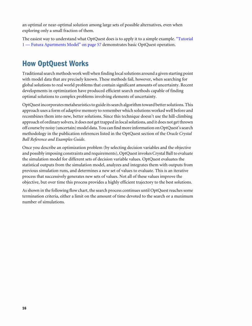
Once you describe an optimization problem (by selecting decision variables and the objectiveand possibly imposing constraints and requirements), OptQuest invokes Crystal Ball to evaluatethe simulation model for different sets of decision variable values. OptQuest evaluates thestatistical outputs from the simulation model, analyzes and integrates them with outputs fromprevious simulation runs, and determines a new set of values to evaluate. This is an iterativeprocess that successively generates new sets of values. Not all of these values improve theobjective, but over time this process provides a highly efficient trajectory to the best solutions.
As shown in the following flow chart, the search process continues until OptQuest reaches sometermination criteria, either a limit on the amount of time devoted to the search or a maximumnumber of simulations.
16
Figure 1 OptQuest Flow
About Optimization ModelsIn today's competitive global economy, people are faced with many difficult decisions. Suchdecisions may involve thousands or millions of potential alternatives. A model can providevaluable assistance in analyzing decisions and finding good solutions. Models capture the mostimportant features of a problem and present them in a form that is easy to interpret. Modelsoften provide insights that intuition alone cannot.
An OptQuest optimization model has four major elements: an objective, optional requirements,Crystal Ball decision variables, and optional constraints.
l Optimization Objectives—Elements that represents the target goal of the optimization, suchas maximizing profit or minimizing cost, based on a forecast and related decision variables.
l Requirements—Optional restrictions placed on forecast statistics. All requirements mustbe satisfied before a solution can be considered feasible.
l Decision Variables—Variables over which you have control; for example, the amount ofproduct to make, the number of dollars to allocate among different investments, or whichprojects to select from among a limited set.
l Constraints—Optional restrictions placed on decision variable values. For example, aconstraint may ensure that the total amount of money allocated among various investments
17
cannot exceed a specified amount, or at most one project from a certain group can beselected.
For direct experience in setting up a model and running an optimization, see “Tutorial 2 —Portfolio Allocation Model ” on page 63.
Optimization ObjectivesEach optimization model has one objective that mathematically represents the model’s goal asa function of the assumption and decision variable cells, as well as other formulas in the model.OptQuest’s job is to find the optimal value of the objective by selecting and improving differentvalues for the decision variables.
When model data are uncertain and can only be described using probability distributions, theobjective itself will have some probability distribution for any set of decision variables. You canfind this probability distribution by defining the objective as a forecast and using Crystal Ball tosimulate the model.
Forecast StatisticsYou cannot use an entire forecast distribution as the objective, but must characterize thedistribution using a single summary measure for comparing and selecting one distribution overanother. So, to use OptQuest, you must select a statistic of one forecast to be the objective. Youmust also select whether to maximize or minimize the objective, or set it to a target value.
The statistic you select depends on your goals for the objective. For maximizing or minimizingsome quantity, the mean or median are often used as measures of central tendency, with themean being the more common of the two. For highly skewed distributions, however, the meanmay become the less stable (having a higher standard error) of the two, and so the medianbecomes a better measure of central tendency.
The X in Y Chance statistic can be used only for requirements, not objectives.
For minimizing overall risk, the standard deviation and the variance of the objective are the twobest statistics to use. For maximizing or minimizing the extreme values of the objective, a lowor high percentile may be the appropriate statistic. For controlling the shape or range of theobjective, the skewness, kurtosis, or certainty statistics may be used. If you are working with SixSigma or another process quality program, you may want to use process capability metrics indefining the objective. For more information on these statistics, see the Glossary, online help,and the online Oracle Crystal Ball Statistical Guide.
Minimizing or MaximizingWhether you want to maximize or minimize the objective depends on which statistic you selectto optimize. For example, if your forecast is profit and you select the mean as the statistic, youwould want to maximize the profit mean. However, if you select the standard deviation as thestatistic, you may want to minimize it to limit the uncertainty of the forecast.
18
RequirementsRequirements restrict forecast statistics. These differ from constraints, since constraints restrictdecision variables (or relationships among decision variables). Requirements are sometimescalled probabilistic constraints, chance constraints, side constraints, or goals in other literature.
When you define a requirement, you first select a forecast (either the objective forecast or anotherforecast). As with the objective, you then select a statistic for that forecast, but instead ofmaximizing or minimizing it, you give it an upper bound, a lower bound, or both (a range).
If you want to perform an Efficient Frontier analysis, you can define requirements with variablebounds. For more information, see “Efficient Frontier Analysis” on page 21.
Requirement ExamplesIn the Portfolio Allocation example of Chapter 4, “OptQuest Tutorials,” the investor wants toimpose a condition that limits the standard deviation of the total return. Because the standarddeviation is a forecast statistic and not a decision variable, this restriction is a requirement.
The following are some examples of requirements on forecast statistics that you could specify:
95th percentile >= 1000
-1 <= skewness <= 1
Range 1000 to 2000 >= 50% certainty
Decision VariablesDecision variables are variables in your model that you can control, such as how much rent tocharge or how much money to invest in a mutual fund. Decision variables aren’t required forCrystal Ball models, but are required for OptQuest models. You define decision variables inCrystal Ball by clicking the Define Decision button in the Crystal Ball ribbon.
When you define a decision variable in Crystal Ball, you define its:
l Bounds—Defines the upper and lower limits for the variable. OptQuest searches forsolutions for the decision variable only within these limits.
l Type—Defines whether the variable type is discrete, continuous, binary, category, orcustom:
m Continuous — A variable that can be fractional (that is, it is not required to be an integerand can take on any value between its lower and upper bounds; no step size is requiredand any given range contains an infinite number of possible values.
m Discrete — A variable that can only assume values equal to its lower bound plus amultiple of its step size; a step size is any number greater than zero but less than thevariable's range.
m Binary — A decision variable that can be is 0 or 1 to represent a yes-no decision, where0 = no and 1 = yes.
19
m Category — A decision variable for representing attributes and indexes; can assume anydiscrete integer between the lower and upper bounds (inclusive), where the order (ordirection) of the values does not matter (nominal). The bounds must be integers.
m Custom — A decision variable that can assume any value from a list of specific values(two values or more). You can enter a list of values or a cell reference to a list of valuesin the spreadsheet. If a cell reference is used, it must include more than one cell so therewill be two or more values. Blanks and non-numeric values in the range are ignored. Ifyou enter values in a list, they should be separated by a valid list separator -- a comma,semicolon, or other value specified in the Windows regional and language settings.
For details, refer to the Oracle Crystal Ball User's Guide.
l Step Size—Defines the difference between successive values of a discrete decision variablein the defined range. For example, a discrete decision variable with a range of 1 to 5 and astep size of 1 can only take on the values 1, 2, 3, 4, or 5; a discrete decision variable with arange of 0 to 2 with a step size of 0.25 can only take on the values 0, 0.25, 0.5, 0.75, 1.0, 1.25,1.5, 1.75, and 2.0.
The cell value becomes the base case value, or starting value for the optimization.
Note: If changing the type of a decision variable causes the base case to fall outside the range ofvalues that are valid for that type, a new base case value is selected. The base case changesto the nearest acceptable value for the new type.
In an optimization model, you select which decision variables to optimize from a list of all thedefined decision variables. The values of the decision variables you select will change with eachsimulation until the best value for each decision variable is found within the available time orsimulation limit.
ConstraintsConstraints are optional settings in an optimization model. They restrict the decision variablesby defining relationships among them. For example, if the total amount of money invested intwo mutual funds must be $50,000, you can define this as:
mutual fund #1 + mutual fund #2 = 50000
OptQuest only considers combinations of values for the two mutual funds whose sum is $50,000.
Or if your budget restricts your spending on gasoline and fleet service to $2,500, you can definethis as:
gasoline + service <= 2500
In this case, OptQuest considers only combinations of values for gasoline and service at or lessthan $2,500.
Not all optimization models need constraints.
20
Model and Solution FeasibilityA feasible solution is one that satisfies all defined constraints and requirements. A solution isinfeasible when no combination of decision variable values can satisfy the entire set ofrequirements and constraints. Notice that a solution (i.e., a single set of values for the decisionvariables) can be infeasible by failing to satisfy the problem requirements or constraints, but thisdoesn’t imply that the problem or model itself is infeasible.
However, constraints and requirements can be defined in such a way that the entire model isinfeasible. For example, suppose that in the Portfolio Allocation problem in Chapter 1, theinvestor insists on finding an optimal investment portfolio with the following constraints:
Income fund + Aggressive growth fund <= 10000
Income fund + Aggressive growth fund >= 12000
Clearly, no combination of investments exists that will make the sum of the income fund andaggressive growth fund no more than $10,000 and at the same time greater than or equal to$12,000.
Or, for this same example, suppose the bounds for a decision variable were:
$15,000 <= Income fund <= $25,000
And a constraint was:
Income fund <= 5000
This also results in an infeasible problem.
You can make infeasible problems feasible by fixing the inconsistencies of the relationshipsmodeled by the constraints. OptQuest detects optimization models that are constraint-infeasibleand reports them to you.
If a model is constraint-feasible, OptQuest will always find a feasible solution and search for theoptimal solution (that is, the best solution that satisfies all constraints).
When an optimization model includes requirements, a solution that is constraint-feasible maybe infeasible with respect to one or more requirements.
After first satisfying constraint feasibility, OptQuest assumes that the user's next highest priorityis to find a solution that is requirement-feasible. Therefore, it concentrates on finding arequirement-feasible solution and then on improving this solution, driven by the objective inthe model.
Efficient Frontier AnalysisEfficient Frontier analysis calculates the curve that plots an objective value against changes to arequirement or constraint. A typical use is for comparing portfolio returns against different risklevels so that investors can maximize return and minimize risk. If you want to use this type ofanalysis, you need to define a range of values for a requirement or constraint bound. Forinstructions and more information, see “Setting Up Efficient Frontier Analysis in OptQuest” onpage 53.
21
One use for Efficient Frontier analysis is to allocate funds among a portfolio of investments inthe most efficient way. The Description page of Portfolio Revisited EF.xlsx describes thistechnique. “Efficient Portfolios” on page 22, following, offers the concepts behind it.
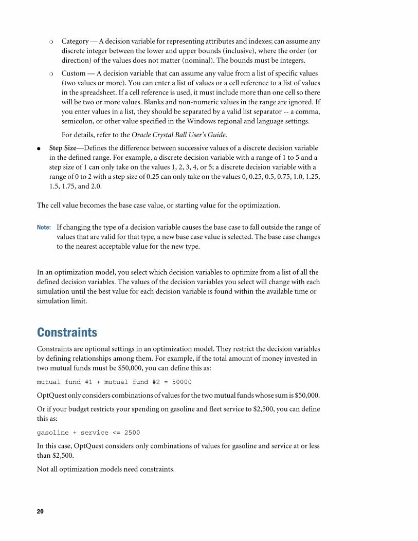
Efficient PortfoliosIf you were to examine all the possible combinations of investment strategies for the assetsdescribed for Portfolio Revisited.xlsx, you would notice that each portfolio had a specific meanreturn and standard deviation of return associated with it. Plotting the means on one axis andthe standard deviations on another axis, you can create a graph like this:
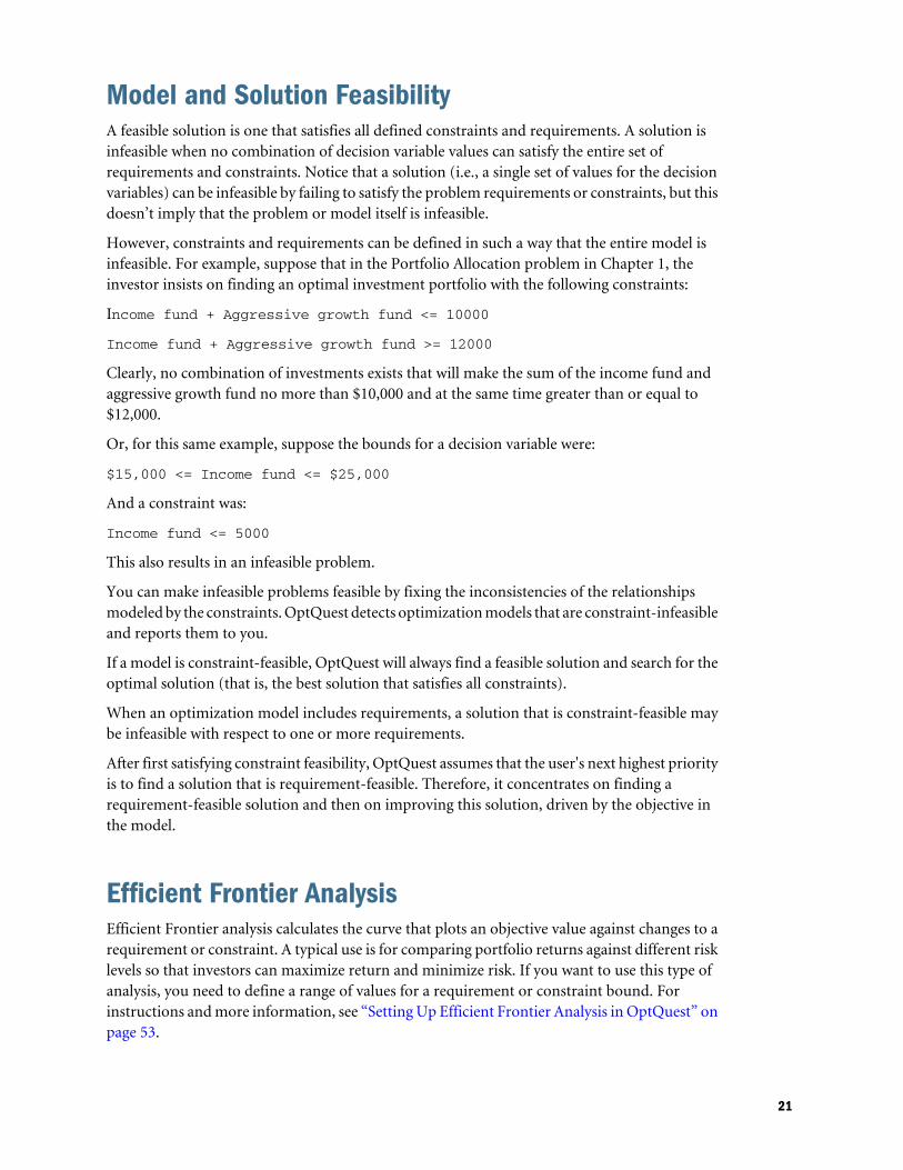
Points on or under the curve (values lower than the curve) represent possible combinations ofinvestments. Points above the curve (values higher than the curve) are unobtainablecombinations given the particular set of assets available. For any given mean return, one portfoliohas the smallest standard deviation possible. This portfolio lies on the curve at the point thatintersects the mean of return.
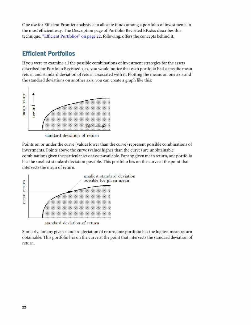
Similarly, for any given standard deviation of return, one portfolio has the highest mean returnobtainable. This portfolio lies on the curve at the point that intersects the standard deviation ofreturn.
22
Portfolios that lie directly on the curve are called efficient (see Markowitz, 1991 listed in thepublication references in the OptQuest section of the Oracle Crystal Ball Reference and ExamplesGuide), since it is impossible to obtain higher mean returns without generating higher standarddeviations, or lower standard deviations without generating lower mean returns. The curve ofefficient portfolios is often called the efficient frontier.
Portfolios with values lower than the curve are called inefficient, meaning better portfolios existwith either higher returns, lower standard deviations, or both.
The example in “Tutorial 2 — Portfolio Allocation Model ” on page 63 uses one technique tosearch for optimal solutions on the efficient frontier. This method uses the mean and standarddeviation of returns as the criteria for balancing risk and reward.
You can also use other criteria for selecting portfolios. Instead of using the mean return, youcould select the median or mode as the measure of central tendency. These selection criteriawould be called median-standard deviation efficient or mode-standard deviation efficient.Instead of using the standard deviation of return, you could select the variance, range minimum,or low-end percentile as the measure of risk or uncertainty. These selection criteria would bemean-variance efficient, mean-range minimum efficient, or mean-percentile efficient.
The mode is usually only available for discrete-valued forecast distributions where distinct valuesmay occur more than once during the simulation.
OptQuest and Process CapabilityYou can use OptQuest to support process capability programs such as Six Sigma, Design for SixSigma (DFSS), Lean principles, and similar quality initiatives. To do this, activate the CrystalBall process capability features by selecting Calculate Capability Metrics on the Statistics tab ofthe Run Preferences dialog. Once you do that, define a lower specification limit (LSL), upperspecification limit (USL), or both for a forecast in the Define Forecast dialog. (You can alsodefine an optional value target.)
Once you have defined at least one of the specification limits, you can optimize capability metricsfor that forecast. The process capability metrics are displayed with other forecast statistics in theOptQuest Objectives panel. When you copy the values back to the model, the optimized values,relevant forecast charts, and the capability metrics table are displayed in the workbook. See theOracle Crystal Ball User's Guide for more information.
23

24
3Setting Up and Optimizing a
Model
In This Chapter
Introduction... . . . . . . . . . . . . . . . . . . . . . . . . . . . . . . . . . . . . . . . . . . . . . . . . . . . . . . . . . . . . . . . . . . . . . . . . . . . . . . . . . . . . . . . . . . . . . .25
Overview ... . . . . . . . . . . . . . . . . . . . . . . . . . . . . . . . . . . . . . . . . . . . . . . . . . . . . . . . . . . . . . . . . . . . . . . . . . . . . . . . . . . . . . . . . . . . . . . . . .25
Developing a Crystal Ball Optimization Model .. . . . . . . . . . . . . . . . . . . . . . . . . . . . . . . . . . . . . . . . . . . . . . . . . . . . . . . . .26
Starting OptQuest .. . . . . . . . . . . . . . . . . . . . . . . . . . . . . . . . . . . . . . . . . . . . . . . . . . . . . . . . . . . . . . . . . . . . . . . . . . . . . . . . . . . . . . . . .28
Selecting the Forecast Objective .. . . . . . . . . . . . . . . . . . . . . . . . . . . . . . . . . . . . . . . . . . . . . . . . . . . . . . . . . . . . . . . . . . . . . . . .28
Selecting Decision Variables to Optimize ... . . . . . . . . . . . . . . . . . . . . . . . . . . . . . . . . . . . . . . . . . . . . . . . . . . . . . . . . . . . . .30
Specifying Constraints . . . . . . . . . . . . . . . . . . . . . . . . . . . . . . . . . . . . . . . . . . . . . . . . . . . . . . . . . . . . . . . . . . . . . . . . . . . . . . . . . . . .31
Setting Options... . . . . . . . . . . . . . . . . . . . . . . . . . . . . . . . . . . . . . . . . . . . . . . . . . . . . . . . . . . . . . . . . . . . . . . . . . . . . . . . . . . . . . . . . . .40
Running Optimizations... . . . . . . . . . . . . . . . . . . . . . . . . . . . . . . . . . . . . . . . . . . . . . . . . . . . . . . . . . . . . . . . . . . . . . . . . . . . . . . . . . .42
Interpreting the Results.. . . . . . . . . . . . . . . . . . . . . . . . . . . . . . . . . . . . . . . . . . . . . . . . . . . . . . . . . . . . . . . . . . . . . . . . . . . . . . . . . . .48
Saving Optimization Models and Settings ... . . . . . . . . . . . . . . . . . . . . . . . . . . . . . . . . . . . . . . . . . . . . . . . . . . . . . . . . . . . .53
Closing OptQuest.. . . . . . . . . . . . . . . . . . . . . . . . . . . . . . . . . . . . . . . . . . . . . . . . . . . . . . . . . . . . . . . . . . . . . . . . . . . . . . . . . . . . . . . . . .53
Setting Up Efficient Frontier Analysis in OptQuest .. . . . . . . . . . . . . . . . . . . . . . . . . . . . . . . . . . . . . . . . . . . . . . . . . . . . .53
Transferring Settings from .opt Files.. . . . . . . . . . . . . . . . . . . . . . . . . . . . . . . . . . . . . . . . . . . . . . . . . . . . . . . . . . . . . . . . . . . . .54
Learning More About OptQuest .. . . . . . . . . . . . . . . . . . . . . . . . . . . . . . . . . . . . . . . . . . . . . . . . . . . . . . . . . . . . . . . . . . . . . . . . . .56
IntroductionThis chapter describes how to use OptQuest, step by step. It also gives details about each of thepanels and dialogs in OptQuest.
Overview
ä To set up and optimize a model with OptQuest, follow these steps:
1 Create a Crystal Ball model of the problem.
2 Define the decision variables within Crystal Ball.
3 In OptQuest, select the forecast objective and define any requirements.
4 Select decision variables to optimize.
5 Specify any constraints on the decision variables.
6 Select optimization settings.
25
7 Run the optimization.
8 Interpret the results.
For Users of OptQuest Versions Earlier Than 11.1.1.xIf you used a version of OptQuest earlier than 11.1.1.x, be aware of some significant changes. Asyou have discovered, the user interface is redesigned to be easier to use. For added flexibility,there are now five types of decision variables.
Another difference is that .opt files are no longer used to store optimization settings. For moreinformation on saving optimization settings and options, see “Saving Optimization Models andSettings” on page 53. An .opt file viewer is provided to help you transfer settings from .opt filesto current model workbooks. For instructions, see “Transferring Settings from .opt Files” onpage 54.
Developing a Crystal Ball Optimization ModelBefore using OptQuest, you must first develop a useful Crystal Ball model. This involves buildinga well-tested spreadsheet in Microsoft Excel, and then defining assumptions and forecast cellsusing Crystal Ball. You should refine the Crystal Ball model and run several simulations to ensurethat the model is working correctly and that the results are what you expect.
Developing the WorksheetYou should build your spreadsheet model using principles of good design, since this makesunderstanding and modifying it easier.
The spreadsheet should include:
l A descriptive title.
l An input data area separate from the output and any working space. Place all input variablesin their own cells where you can later define them as assumptions or decision variables.
l A working space for all complex calculations, formulas, and data tables.
l A separate output section that provides the model results.
Examine the Portfolio Allocation spreadsheet model (Figure 23) for an example.
Notice that all assumptions are in rows 5 through 8. Rows 13 through 16 are reserved for decisionvariables, created by users during the OptQuest tutorials. Forecast cells reference these inputvariable cells in their calculations, not values directly. Therefore, you could easily change anyvalues, and the forecast calculations would be automatically updated.
Other tips that improve the usefulness of your spreadsheet are:
l Reference input data only with cell references or range names so that any changes areautomatically reflected throughout the worksheet.
26
l Use formats, such as currency or comma formats, appropriately.
l Divide complex calculations into several cells to minimize the chance for error and enhanceunderstanding.
l Place comments next to formula cells for explanation, if needed.
l Consult a reference such as those listed in the publication references in the OptQuest sectionof the Oracle Crystal Ball Reference and Examples Guide for further discussion of goodspreadsheet design.
Defining Assumptions, Decision Variables, and ForecastsOnce you build and test the spreadsheet, you can define your assumptions, decision variables,and forecasts. For more information on defining assumptions, decision variables, and forecasts,see the Oracle Crystal Ball User's Guide.
Setting Crystal Ball Run PreferencesTo set Crystal Ball run preferences, select Run Preferences in the Oracle Crystal Ball ribbon. Foroptimization purposes, you should usually use the following Crystal Ball settings:
l Trials tab — Maximum number of trials to run set to 1000.
Central-tendency statistics such as mean, median, and mode usually stabilize sufficiently at500 to 1000 trials per simulation. Tail-end percentiles and maximum and minimum rangevalues generally require at least 2000 trials.
l Sampling tab — Sampling method set to Latin Hypercube with the default bin size.
Latin Hypercube sampling increases the quality of the solutions, especially the accuracy ofthe mean statistic.
l Sampling tab — Random Number Generation set to Use Same Sequence Of RandomNumbers with an Initial Seed Value of 999.
The initial seed value determines the first number in the sequence of random numbersgenerated for the assumption cells. Then, you can repeat simulations using the same set ofrandom numbers to accurately compare the simulation results. If you do not set an initialseed value, OptQuest will automatically pick a random seed and use that starting seed foreach simulation that is run.
When your Crystal Ball forecast has extreme outliers, run the optimization with severaldifferent seed values to test the solution’s stability.
l Speed tab — Run in Normal Speed.
After you define the assumptions, decision variables, and forecasts in Crystal Ball, you can beginthe optimization process in OptQuest.
27
Starting OptQuest
ä To start OptQuest:
1 Select OptQuest in the Crystal Ball ribbon.
The OptQuest wizard starts.
2 Set up the optimization by completing each wizard panel. The first step of this process is selecting aforecast objective to optimize.
Note: This version of OptQuest does not use .opt files. If you would like to retrieve settingsfrom existing .opt files for use in this version of OptQuest, see “Transferring Settingsfrom .opt Files” on page 54.
Selecting the Forecast Objective When the OptQuest wizard starts, the Objectives panel opens, similar to Figure 15. (The firsttime you start the wizard, the Welcome screen opens. Click Next to display the Objectives panel.)
In the Objectives panel, you select a forecast statistic to maximize, minimize, or set to a targetvalue. Optionally, you can define one or more requirements either on the objective forecast oron other forecasts.
Figure 24 shows a default objective including the first forecast found in the model.
Note: You can define more than one objective but can use only one at a time. Select Exclude toeliminate an objective from the current optimization.
ä To define a forecast objective and, optionally, define requirements:
1 If you have more than one workbook open, use the Primary workbook list to select the workbook withdata to optimize.
2 Click Add Objective.
A default objective is displayed in the Objectives area.
3 Review the default objective definition. It has the format Operation, Statistic, Forecast.
a. First, if the model has more than one forecast, does the default objective include thesame forecast you want to include in the objective? If not, click the underlined forecastand replace it with your selection. If more than ten forecasts are available, MoreForecasts is displayed at the bottom of the list. You can select it to display a forecastselection dialog.
b. Next, do you want to maximize a statistic for that forecast? If you would prefer tominimize the statistic or set it to a target value, click the underlined operation and selectan alternative.
28
c. Finally, is the underlined statistic the one you prefer to use. If not, click it and select adifferent one. If you have activated Crystal Ball’s process capability features and havedefined an LSL or USL, the process capability statistics are available in the list of statistics.
Note: For many problems, the mean (expected value) of the forecast is the mostappropriate statistic to optimize, but it need not always be. For example, investorswho want to maximize the upside potential of their portfolios may want to usethe 90th or 95th percentile as the objective. The results would be solutions thathave the highest likelihood of achieving the largest possible returns. Similarly, tominimize the downside potential of the portfolio, they may use the 5th or 10thpercentile as the objective to minimize the possibility of large losses. You can useother statistics to realize different objectives. See the Glossary, online help, andthe online Oracle Crystal Ball Statistical Guide for a description of all availablestatistics.
4 Optional: Define requirements.
a. To add a requirement, click Add Requirement. A default requirement is displayed.
b. First, look at the default statistic. Is it the one you want to use? To review the list ofavailable choices, click the underlined statistic and select a different one if you want.Depending on your choice, the requirement statement could change.
c. Next, review the forecast. If you want, click the underlined forecast and select another.
d. Then, review the requirement operator. The selected statistic can be less than or equalto a selected value, greater than or equal to a selected value, or between two selectedvalues (including the values). Click the underlined limit to select another. If you selectBetween, an additional target value is displayed.
e. Finally, review and adjust the target value or values. To change a value, click it and thentype a new number over it.
f. You can repeat steps3a through 3e to add additional requirements. New requirementsare duplicates of the last one entered.
g. Optional: If you want to set variable bounds for Efficient Frontier analysis, select avariable and click Efficient Frontier. For details, see “Efficient Frontier Analysis” on page21.
Note: You can create multiple requirements without using all of them at once. If you selectExclude, that requirement is not used in the current OptQuest optimization.
5 Optional: If you have an .opt file from an earlier version of OptQuest, click Import to open the file forassistance in defining new objectives, requirements, and constraints. For details, see “TransferringSettings from .opt Files” on page 54.
6 Optional: To delete a requirement, click it and then click Delete.
7 When objective and requirement settings are complete, click Next.
The Decision Variables panel opens.
29
Selecting Decision Variables to OptimizeWhen you click Next in the Objectives panel, the Decision Variables panel opens, similar toFigure 25. It lists every decision variable, frozen or not, defined in all open Microsoft Excelworkbooks.
The next step of the optimization process is selecting decision variables to optimize. The valueof each decision variable changes with each simulation until OptQuest finds values that yieldthe best objective. For some analyses, you may fix the values of certain decision variables andoptimize the rest.
By default, all decision variables in all open workbooks are shown, even those that are frozen inyour model. Frozen decision variables have a check in the Freeze column. If you want, you canclear them and include them in the optimization. Be aware, though, that if you freeze or unfreezea decision variable, you are also changing it in your model.
OptQuest uses the limits, base case (start value), and decision variable type you entered whenyou defined the decision variables.
If you select Show Cell Locations, the following additional columns are displayed in the DecisionVariables panel: Cell Address, Worksheet, and Workbook.
ä To confirm and change selections:
1 Review the listed variables. Select Freeze for any that you do not want to include in the OptQuestoptimization.
2 Optional: Change the lower and upper bounds, base case, or decision variable type for any listed decisionvariable. Highlight the existing value and type over it. This changes the decision variable definition inyour worksheet.
Notice the following about these settings:
l The tighter the bounds you specify, the fewer values OptQuest must search to find theoptimal solution. However, this efficiency comes at the expense of missing the optimalsolution if it lies outside the specified bounds.
l By default, OptQuest uses the base case cell values in your Crystal Ball model as thesuggested starting solution. If the suggested values lie outside of the specified boundsor do not meet the problem constraints, OptQuest ignores them.
Note: You can sort decision variables in the Decision Variables panel by name, type,freeze status, cell address, worksheet, or workbook. To sort, click the columnheading. An arrow is displayed to show the direction of the sort. The sort columnand direction of the decision variables is stored as a global preference and is alsoused to set the order of the decision variables in the reports and extracted data.
3 When your decision variable selections are complete, click Next.
The Constraints panel opens.
30
Specifying Constraints In OptQuest, constraints limit the possible solutions to a model in terms of relationships amongthe decision variables. You can use the Constraints panel to specify linear and nonlinearconstraints. For example, in “Tutorial 2 — Portfolio Allocation Model ” on page 63, the totalinvestment was limited to $100,000. In the Constraints panel, this limit is expressed by theformula:
Money Market fund + Income fund + Growth and Income fund + Aggressive
Growth fund = 100000
By default, the Constraints panel opens in Simple Entry mode. In this mode, most of theconstraint formula is entered into cells in your spreadsheet. You then complete the constraintformula on the Constraints panel using a simple conditional expression like Sheet!A1 <=100.
For more information, see the following section, “Specifying Constraints in Simple Entry Mode”on page 31.
If you move to Advanced Entry mode, you can enter constraint formulas directly. See “SpecifyingConstraints in Advanced Entry Mode” on page 31.
Note: You can create multiple constraints without using all of them at once. If you selectExclude, that constraint is not used in the current OptQuest optimization.
You can now create bulk constraints by using cell ranges on either side of the constraintformula in both Simple Entry and Advanced Entry modes (“Using Bulk Constraints” onpage 36).
Specifying Constraints in Simple Entry ModeWhen you click Next in the Decision Variables panel or click Constraints in the navigation list,the Constraints panel opens, similar to Figure 26.
By default, the Constraints panel opens in Simple Entry mode. If you click Add Constraint, youcan reference cells with formulas for the left and right sides of the constraint formula and youcan select an operator. Alternatively, you can enter a value for the right side or left side. Forinformation about allowable constraint formulas, see “Constraint Rules and Syntax” on page34.
For an example of using Simple Entry mode, see “Specifying Constraints” on page 68.
Specifying Constraints in Advanced Entry Mode
ä To use the Constraints panel in Advanced Entry mode:
1 Switch to Advanced Entry mode by selecting Advanced Entry in the corner of the Constraints editor.
2 In the Constraints editor, enter a mathematical formula. You can use the buttons at the bottom of theConstraints panel to help you edit the formula.
31
For information on the Constraints editor syntax, see “Constraint Rules and Syntax” onpage 34.
You can also enter parts of a constraint formula into spreadsheet cells and then referencethose cells, separated by an operator, in a formula. See “Constraints and Cell References inAdvanced Entry Mode” on page 35.
3 Enter any additional constraints on their own lines.
4 When you are done, click Next to display the Options panel.
Note: In Advanced Entry mode, you can use Ctrl+c and Ctrl+v to copy and paste constraintsto duplicate them for further editing. You can also paste formulas from the clipboard,and this is limited to Advanced Entry mode.
Advanced Entry ExampleTo enter Advanced Entry mode, select Advanced Entry in the Constraints panel of the OptQuestwizard. A Constraints edit box opens.
At first the Constraints edit box is blank. A series of buttons near the bottom of the dialog canhelp you create a formula in it. You can enter a linear or nonlinear formula and you can enterany number of formulas, as long as each constraint formula is on its own line. For details, see“Constraints Editor and Related Buttons” on page 33.
In this case, supposed you want to create a formula that adds all the decision variable values andspecifies that they should be equal to $100,000, as discussed in “Tutorial 2 — Portfolio AllocationModel ” on page 63.
Constraints Editor Example
ä To create this formula:
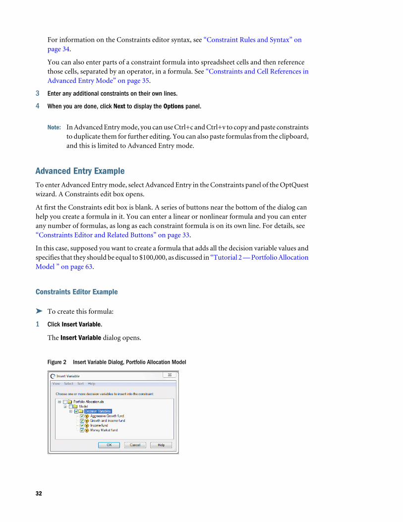
1 Click Insert Variable.
The Insert Variable dialog opens.
Figure 2 Insert Variable Dialog, Portfolio Allocation Model
32
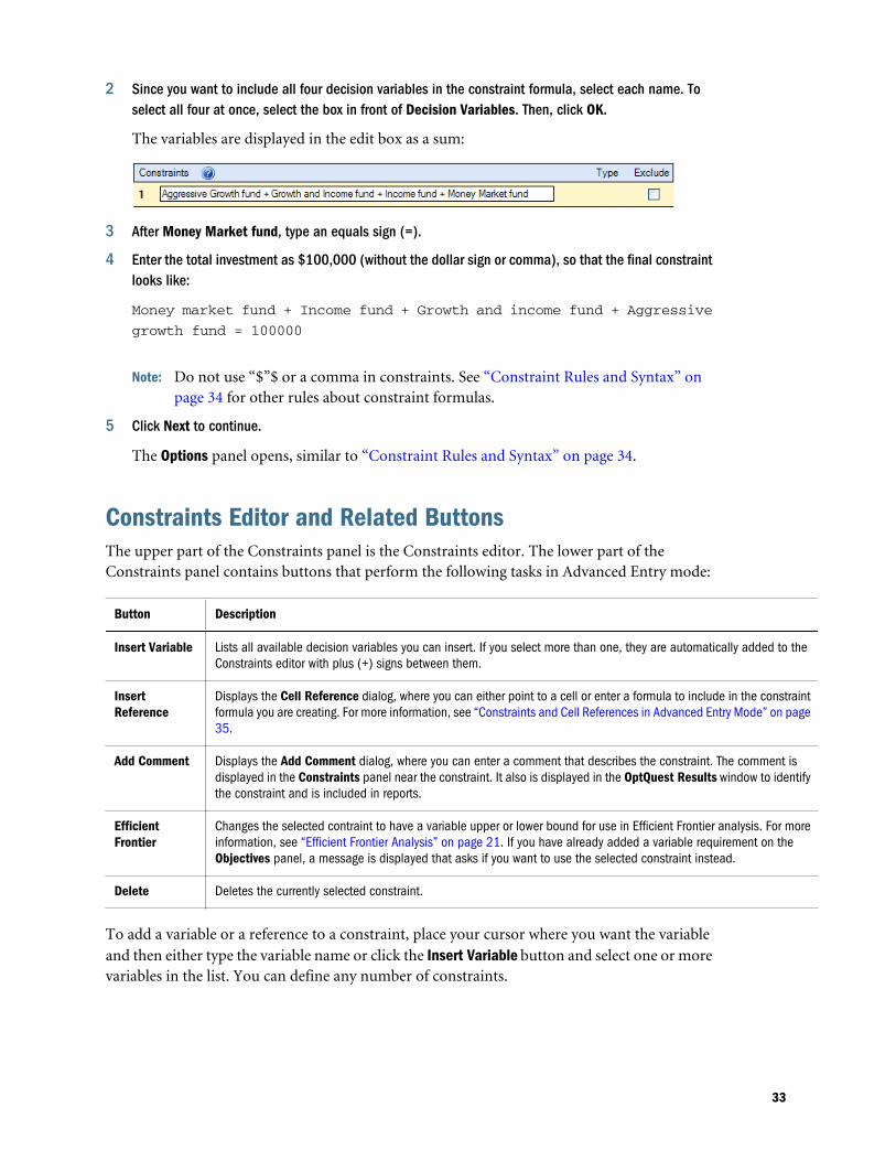
2 Since you want to include all four decision variables in the constraint formula, select each name. Toselect all four at once, select the box in front of Decision Variables. Then, click OK.
The variables are displayed in the edit box as a sum:
3 After Money Market fund, type an equals sign (=).
4 Enter the total investment as $100,000 (without the dollar sign or comma), so that the final constraintlooks like:
Money market fund + Income fund + Growth and income fund + Aggressive
growth fund = 100000
Note: Do not use “$”$ or a comma in constraints. See “Constraint Rules and Syntax” onpage 34 for other rules about constraint formulas.
5 Click Next to continue.
The Options panel opens, similar to “Constraint Rules and Syntax” on page 34.
Constraints Editor and Related ButtonsThe upper part of the Constraints panel is the Constraints editor. The lower part of theConstraints panel contains buttons that perform the following tasks in Advanced Entry mode:
Button Description
Insert Variable Lists all available decision variables you can insert. If you select more than one, they are automatically added to theConstraints editor with plus (+) signs between them.
InsertReference
Displays the Cell Reference dialog, where you can either point to a cell or enter a formula to include in the constraintformula you are creating. For more information, see “Constraints and Cell References in Advanced Entry Mode” on page35.
Add Comment Displays the Add Comment dialog, where you can enter a comment that describes the constraint. The comment isdisplayed in the Constraints panel near the constraint. It also is displayed in the OptQuest Results window to identifythe constraint and is included in reports.
EfficientFrontier
Changes the selected contraint to have a variable upper or lower bound for use in Efficient Frontier analysis. For moreinformation, see “Efficient Frontier Analysis” on page 21. If you have already added a variable requirement on theObjectives panel, a message is displayed that asks if you want to use the selected constraint instead.
Delete Deletes the currently selected constraint.
To add a variable or a reference to a constraint, place your cursor where you want the variableand then either type the variable name or click the Insert Variable button and select one or morevariables in the list. You can define any number of constraints.
33
Constraint Rules and SyntaxIn general, constraint formulas are like standard Microsoft Excel formulas. Each constraintformula:
l Is constructed of mathematical combinations of constants, selected decision variables, andother elements.
l Must each be on its own line.
l Can be linear or nonlinear. You can multiply a decision variable by a constant (linear), andyou can multiply it by another decision variable (nonlinear).
l Cannot have commas, dollar signs, or other non-mathematical symbols.
In Advanced Entry mode, decision variables can be entered directly by name but in Simple Entrymode, they can only be referenced within spreadsheet formulas by cell location or range name.
In Simple Entry mode, cell references and range names cannot be preceded by a minus sign toindicate that they should be subtracted from something unless they are part of a formulaexpression and not an isolated cell reference or range name.
If you are using the cell selector in Simple Entry mode, only simple cell references or range namesare selectable. You cannot include coefficients or mathematical operators.
Normally, constraint formulas should always refer to at least one decision variable, either directlyor indirectly. However, there may be situations where you want to set the value in a constraintformula by some other means (for example, a user-defined macro or some other process). Inthese cases, you should enter the constraint using the form cell_reference < constant. OptQuestidentifies this constraint as a constant type (since it does not include decision variables) and maywarn you that the constraint may result in no feasible solutions if care is not taken.
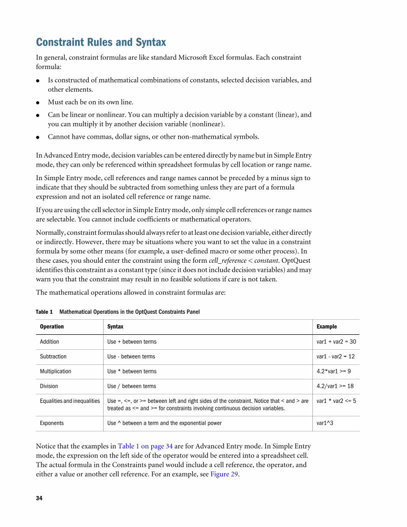
The mathematical operations allowed in constraint formulas are:
Table 1 Mathematical Operations in the OptQuest Constraints Panel
Operation Syntax Example
Addition Use + between terms var1 + var2 = 30
Subtraction Use - between terms var1 - var2 = 12
Multiplication Use * between terms 4.2*var1 >= 9
Division Use / between terms 4.2/var1 >= 18
Equalities and inequalities Use =, <=, or >= between left and right sides of the constraint. Notice that < and > aretreated as <= and >= for constraints involving continuous decision variables.
var1 * var2 <= 5
Exponents Use ^ between a term and the exponential power var1^3
Notice that the examples in Table 1 on page 34 are for Advanced Entry mode. In Simple Entrymode, the expression on the left side of the operator would be entered into a spreadsheet cell.The actual formula in the Constraints panel would include a cell reference, the operator, andeither a value or another cell reference. For an example, see Figure 29.
34
Note: Although these examples always show a formula on the left side of the operator, you canactually have a formula (or a cell reference to a formula in the spreadsheet) on either theleft or the right side.
You can also use Microsoft Excel functions and range names in constraint formulas.
If you are using Advanced Entry mode, calculations occur according to the following precedence:multiplication and division first, and then addition and subtraction. For example,5*E6+10*F7-26*G4 means: Multiply 5 times the value in cell E6, add that product to theproduct of 10 times the value in cell F7, and then subtract the product of 26 times the value incell G4 from the result. You can use parentheses to override precedence. If you are using SimpleEntry mode, you are creating formulas in Microsoft Excel and Microsoft Excel’s precedence rulesapply.
Note: Constraint formulas with cell ranges such as A1:A3 < B1:B3 are now supported inOptQuest. For details, see “Using Bulk Constraints” on page 36.
Constraints and Cell References in Advanced Entry Mode“Specifying Constraints in Simple Entry Mode” on page 31 describes how you can createformulas in spreadsheet cells and then reference them when creating constraints. You can alsouse cell references in Advanced Entry mode to simplify constraint formulas.
ä To do this in Advanced Entry mode:
1 Enter a formula for the left side of the constraint into a spreadsheet cell. The example in “SpecifyingConstraints in Simple Entry Mode” on page 31 has =SUM(C13:C16) entered into cell G13.
2 Consider what to use for the right side of the formula. It can be a single value or a formula that resolvesto a constant.
3 Decide on the relationship between the left and right side: =, <=, >=.
4 Run OptQuest and display the Constraints panel.
5 With the cursor in a constraint formula edit box, click Insert Reference. Point to the cell with the leftside of the formula and then click OK.
6 Following the cell reference, type the relationship operator.
7 Click Insert Reference again and point to the cell for the right side of the formula. Click OK again.Alternately, you can type a numeric value instead of using a cell reference
You can add additional constraints or other OptQuest settings and run the optimization whensettings are complete.
For best results, avoid putting an entire formula, including operator, in a cell and thenreferencing that cell in a constraint formula that tests whether the formula is true or false. Forexample, suppose cell G6 contains =SUM(B2:E2) >= 10. You should avoid defining a constraintas G6 = TRUE. This method does not provide OptQuest with the information it needs to improvethe solution.
35
Instead, you should break up the left-hand and right-hand parts of the equation and make surethe conditional operator (=, >=, <=) is entered in the constraints panel. In this example, cell G6could contain =SUM(B2:E2) and the constraint could be written G6 >= 10.
Constraint TypesConstraints can be linear, nonlinear, constant (in special situations), or mixed:
l Linear constraints are more efficient in generating feasible solutions to try. They are evaluatedby OptQuest before a solution is generated.
l Nonlinear constraints are evaluated by Microsoft Excel before a simulation is run. They maybe slower to evaluate if they contain many Microsoft Excel functions or refer to manyformulas in the spreadsheet. They are less efficient at generating feasible solutions.
l Constant constraints are generally an error unless a user-defined macro or the Crystal BallAuto Extract feature is used to set values in a referenced spreadsheet cell. For more aboutuser-defined macros and constant constraints, see information about the OptQuestDeveloper Kit in the Oracle Crystal Ball Developer's Guide.
l Mixed constraints are a set of bulk constraints that contain constraints of more than onetype.
When you create a constraint, its type is displayed after the formula.
Using Bulk Constraints
Subtopics
l Rules for Bulk Constraints
l Bulk Constraints Example
The bulk constraints feature of Crystal Ball Decision Optimizer enables you to combineconstraints using cell ranges such as A1:A3 < B1:B3. This is a shorthand notation for definingthree constraints: A1 < B1, A2 < B2, A3 < B3.
For rules and an example, see the topics listed at the beginning of this section.
Rules for Bulk ConstraintsConsider the following rules when creating bulk constraints:
l Bulk constraints can be entered in either Basic Entry or Advanced Entry modes.
l The right-hand side of a bulk constraint formula may consist of just a single constant or cellreference instead of a range.
l If two cell ranges are entered, they must have the same number of cells.
l If a blank cell exists in both ranges at the same point, that constraint is ignored.
36
l The Type column displays Linear, Nonlinear, or Constant if the constraints are all the same.Otherwise, the type is Mixed.
l For best performance, cell ranges should contain less than 1,000 cells.
l The Efficient Frontier button is disabled when bulk constraints are selected in theConstraints panel.
l If a bulk constraint formula has errors, an error is displayed in a red icon for the bulkconstraint.
l Each cell range must be contiguous, a single rectangular block of cells.
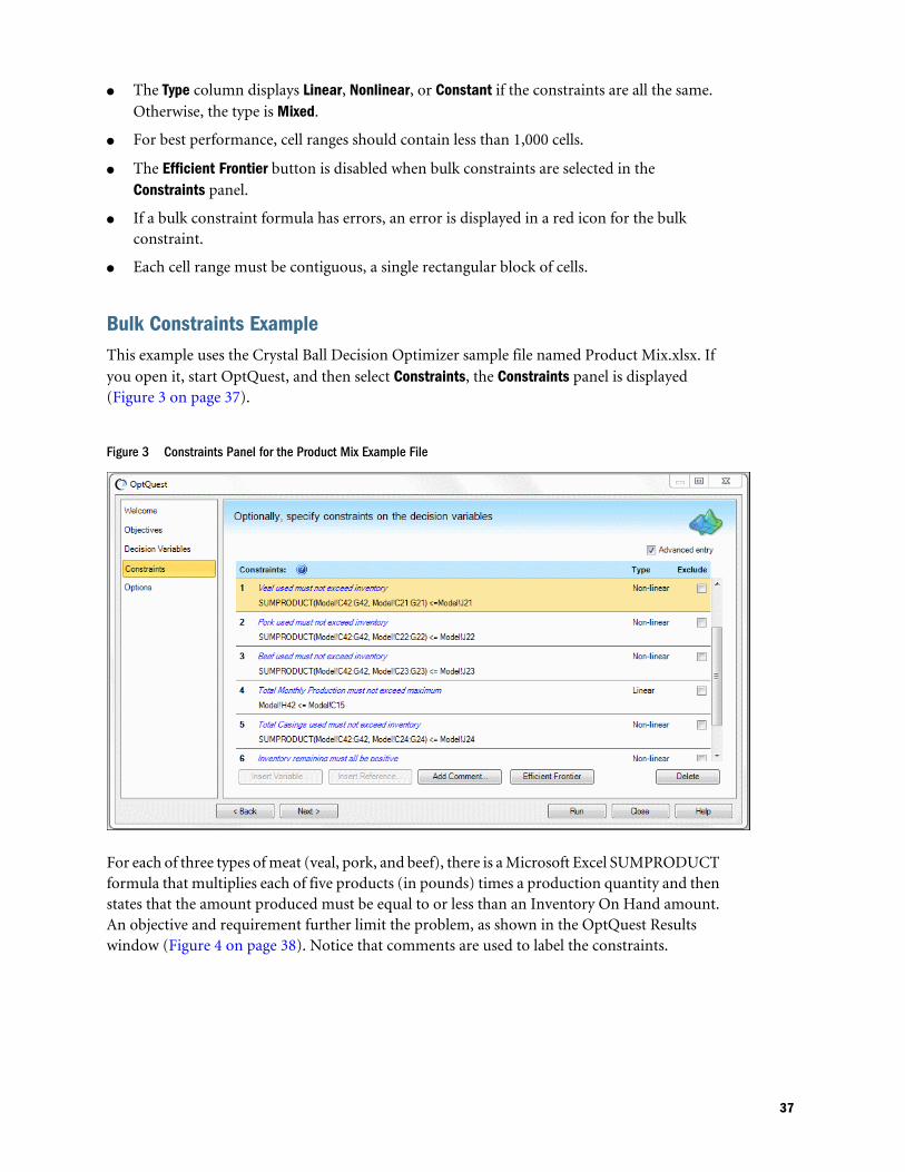
Bulk Constraints ExampleThis example uses the Crystal Ball Decision Optimizer sample file named Product Mix.xlsx. Ifyou open it, start OptQuest, and then select Constraints, the Constraints panel is displayed(Figure 3 on page 37).
Figure 3 Constraints Panel for the Product Mix Example File
For each of three types of meat (veal, pork, and beef), there is a Microsoft Excel SUMPRODUCTformula that multiplies each of five products (in pounds) times a production quantity and thenstates that the amount produced must be equal to or less than an Inventory On Hand amount.An objective and requirement further limit the problem, as shown in the OptQuest Resultswindow (Figure 4 on page 38). Notice that comments are used to label the constraints.
37
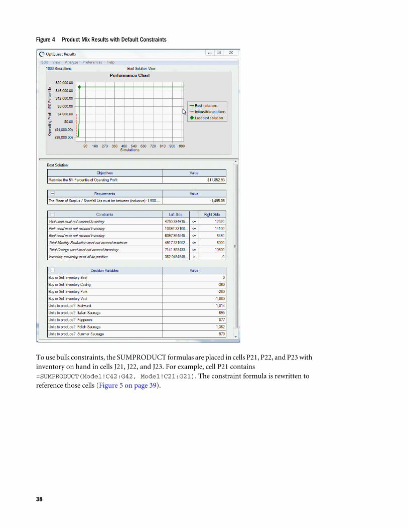
Figure 4 Product Mix Results with Default Constraints
To use bulk constraints, the SUMPRODUCT formulas are placed in cells P21, P22, and P23 withinventory on hand in cells J21, J22, and J23. For example, cell P21 contains=SUMPRODUCT(Model!C42:G42, Model!C21:G21). The constraint formula is rewritten toreference those cells (Figure 5 on page 39).
38
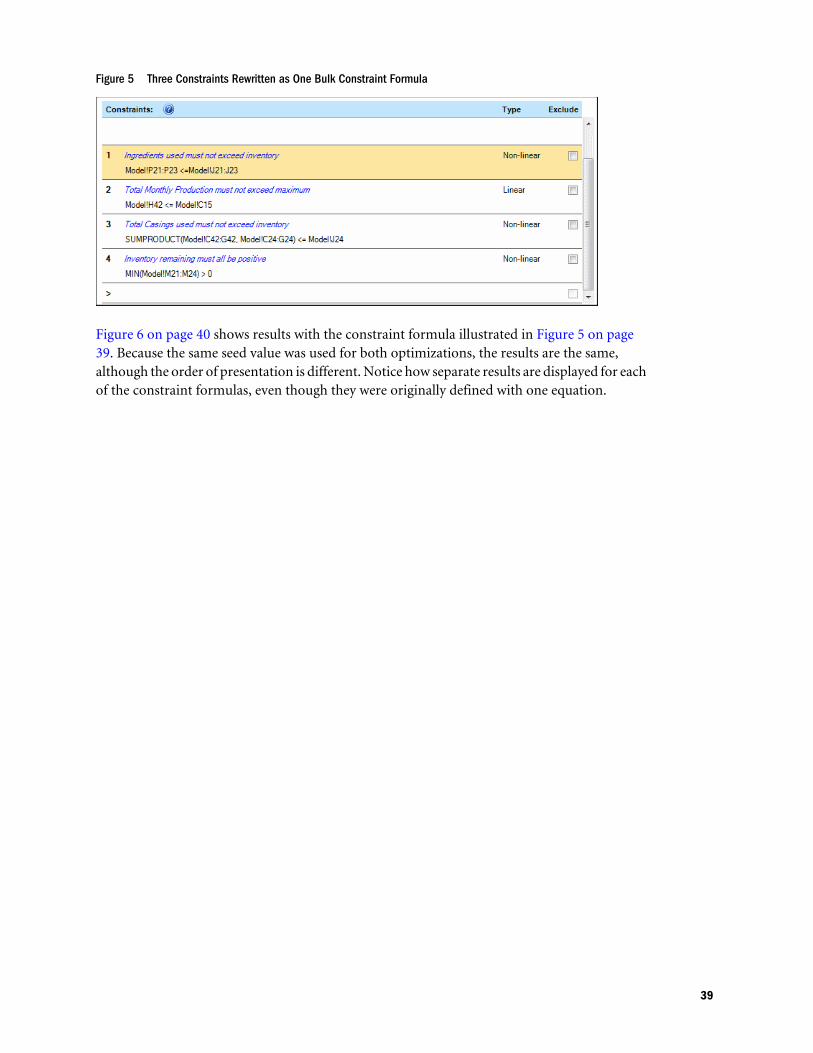
Figure 5 Three Constraints Rewritten as One Bulk Constraint Formula
Figure 6 on page 40 shows results with the constraint formula illustrated in Figure 5 on page39. Because the same seed value was used for both optimizations, the results are the same,although the order of presentation is different. Notice how separate results are displayed for eachof the constraint formulas, even though they were originally defined with one equation.
39
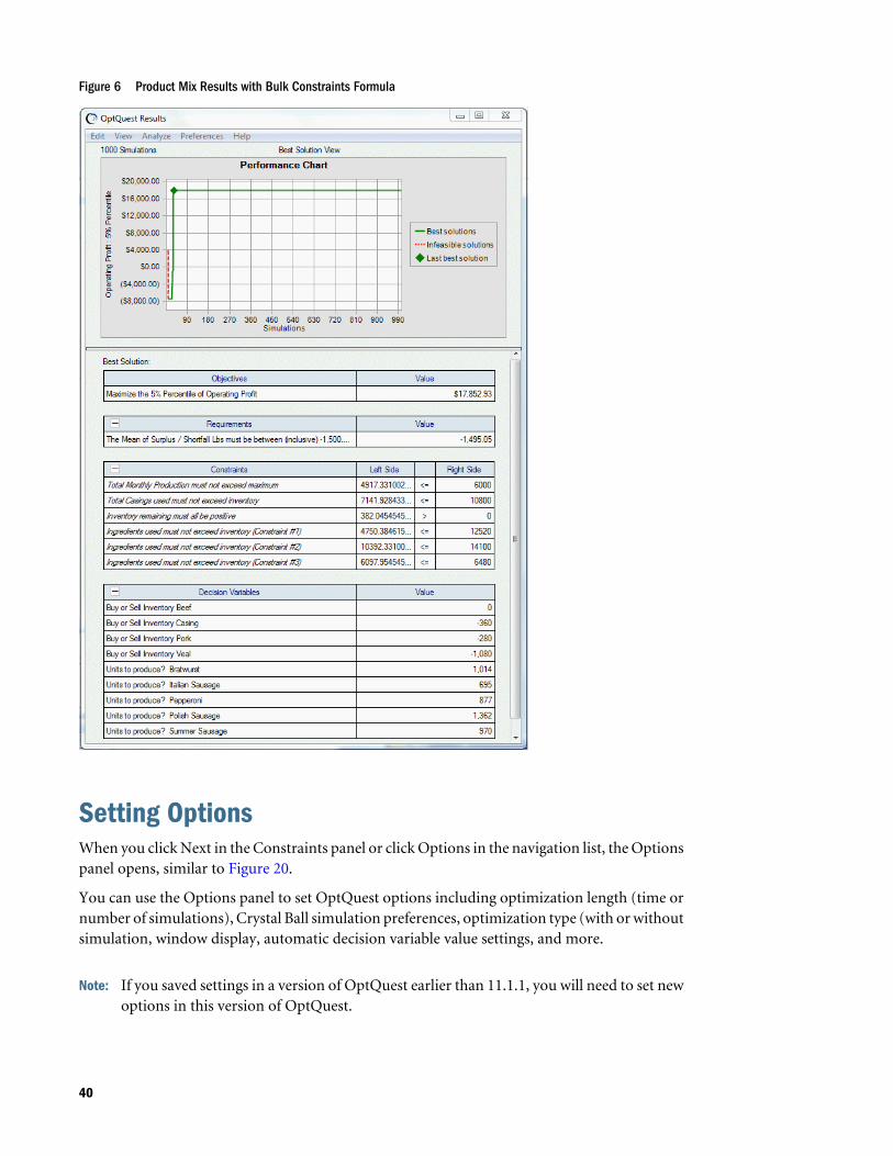
Figure 6 Product Mix Results with Bulk Constraints Formula
Setting OptionsWhen you click Next in the Constraints panel or click Options in the navigation list, the Optionspanel opens, similar to Figure 20.
You can use the Options panel to set OptQuest options including optimization length (time ornumber of simulations), Crystal Ball simulation preferences, optimization type (with or withoutsimulation, window display, automatic decision variable value settings, and more.
Note: If you saved settings in a version of OptQuest earlier than 11.1.1, you will need to set newoptions in this version of OptQuest.
40
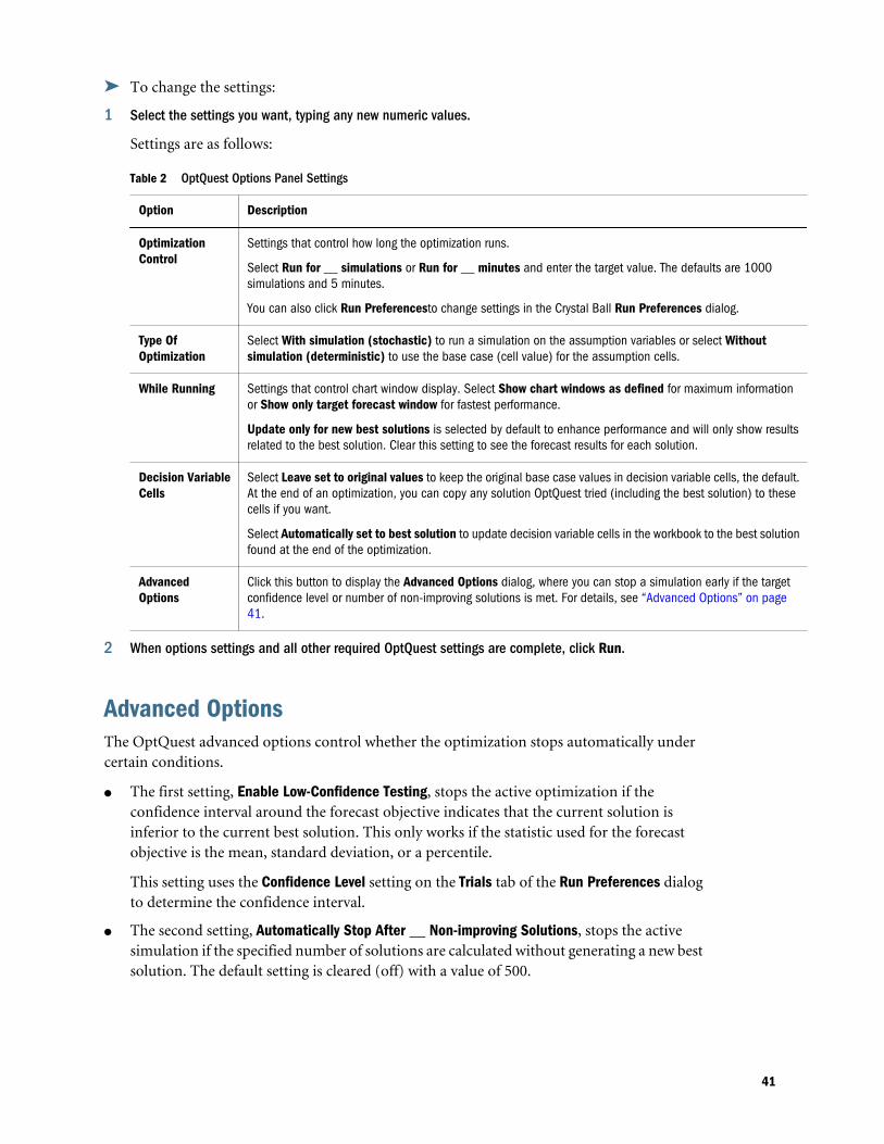
ä To change the settings:
1 Select the settings you want, typing any new numeric values.
Settings are as follows:
Table 2 OptQuest Options Panel Settings
Option Description
OptimizationControl
Settings that control how long the optimization runs.
Select Run for __ simulations or Run for __ minutes and enter the target value. The defaults are 1000simulations and 5 minutes.
You can also click Run Preferencesto change settings in the Crystal Ball Run Preferences dialog.
Type OfOptimization
Select With simulation (stochastic) to run a simulation on the assumption variables or select Withoutsimulation (deterministic) to use the base case (cell value) for the assumption cells.
While Running Settings that control chart window display. Select Show chart windows as defined for maximum informationor Show only target forecast window for fastest performance.
Update only for new best solutions is selected by default to enhance performance and will only show resultsrelated to the best solution. Clear this setting to see the forecast results for each solution.
Decision VariableCells
Select Leave set to original values to keep the original base case values in decision variable cells, the default.At the end of an optimization, you can copy any solution OptQuest tried (including the best solution) to thesecells if you want.
Select Automatically set to best solution to update decision variable cells in the workbook to the best solutionfound at the end of the optimization.
AdvancedOptions
Click this button to display the Advanced Options dialog, where you can stop a simulation early if the targetconfidence level or number of non-improving solutions is met. For details, see “Advanced Options” on page41.
2 When options settings and all other required OptQuest settings are complete, click Run.
Advanced OptionsThe OptQuest advanced options control whether the optimization stops automatically undercertain conditions.
l The first setting, Enable Low-Confidence Testing, stops the active optimization if theconfidence interval around the forecast objective indicates that the current solution isinferior to the current best solution. This only works if the statistic used for the forecastobjective is the mean, standard deviation, or a percentile.
This setting uses the Confidence Level setting on the Trials tab of the Run Preferences dialogto determine the confidence interval.
l The second setting, Automatically Stop After __ Non-improving Solutions, stops the activesimulation if the specified number of solutions are calculated without generating a new bestsolution. The default setting is cleared (off) with a value of 500.
41
Note: When confidence testing is selected, OptQuest can yield different results even when thesame seed is selected. For complete result equivalence from one optimization to the next,do not select Enable Low-Confidence Testing.
Running OptimizationsTo run an optimization, click Run at the bottom of any OptQuest wizard panel. Once theoptimization starts, you can use buttons in the Control Panel to stop, pause, continue, or restartat any time.
You cannot work in Crystal Ball or Microsoft Excel or make changes in OptQuest when runningan optimization, but you can work in other programs. Do not close Microsoft Excel, CrystalBall, or OptQuest while running an optimization.
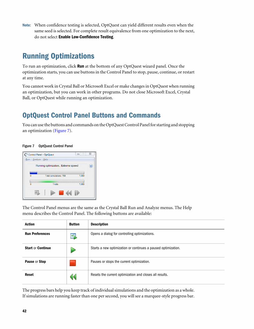
OptQuest Control Panel Buttons and CommandsYou can use the buttons and commands on the OptQuest Control Panel for starting and stoppingan optimization (Figure 7).
Figure 7 OptQuest Control Panel
The Control Panel menus are the same as the Crystal Ball Run and Analyze menus. The Helpmenu describes the Control Panel. The following buttons are available:
Action Button Description
Run Preferences Opens a dialog for controlling optimizations.
Start or Continue Starts a new optimization or continues a paused optimization.
Pause or Stop Pauses or stops the current optimization.
Reset Resets the current optimization and closes all results.
The progress bars help you keep track of individual simulations and the optimization as a whole.If simulations are running faster than one per second, you will see a marquee-style progress bar.
42
If an optimization is set to run for a maximum amount of time, the upper progress bar showselapsed time instead of number of stimulations. A notification message is displayed if theoptimization stops early because a set confidence level is reached or there has been no solutionimprovement for a set number of simulations.
If you click the More button, , a panel opens with additional information about theoptimization.
OptQuest Results WindowWhen an optimization is complete, you can view the OptQuest Results window for informationabout the current optimization. The following sections describe different Results window views:
l “Best Solution View” on page 43
l “Solution Analysis View” on page 45
l “Efficient Frontier Chart” on page 47
Best Solution ViewFigure 8 shows Best Solution view results for an OptQuest example model, Product Mix.xlsx.
43
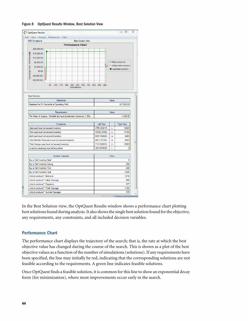
Figure 8 OptQuest Results Window, Best Solution View
In the Best Solution view, the OptQuest Results window shows a performance chart plottingbest solutions found during analysis. It also shows the single best solution found for the objective,any requirements, any constraints, and all included decision variables.
Performance Chart
The performance chart displays the trajectory of the search; that is, the rate at which the bestobjective value has changed during the course of the search. This is shown as a plot of the bestobjective values as a function of the number of simulations (solutions). If any requirements havebeen specified, the line may initially be red, indicating that the corresponding solutions are notfeasible according to the requirements. A green line indicates feasible solutions.
Once OptQuest finds a feasible solution, it is common for this line to show an exponential decayform (for minimization), where most improvements occur early in the search.
44
Best Solution Values
Each time OptQuest identifies a better solution (closer to feasibility or with a better objective)during the optimization, it plots new points in the performance chart and updates the tablesthat accompany the chart.
If you have requested an Efficient Frontier analysis, you can also display the Efficient Frontierview (“Efficient Frontier Analysis” on page 21).
Menus
The OptQuest Results window has several menus you can use to copy results to your spreadsheet,copy charts, print results, view other charts, and more. For a list of menu commands and theirshortcut keys, see the Oracle Crystal Ball Accessibility Guide.
Solution Analysis ViewIn Solution Analysis view, the OptQuest Results window lists the best solutions found duringthe optimization. By default, the top 5% of solutions are sorted by the objective value. Controlsat the bottom of the window indicate how many solutions to view. Statistics are calculated forthe solutions shown.
Note: While OptQuest is running, Solution Analysis view shows the new best solutions, exceptfor Efficient Frontier analyses. The top ten solutions still show when an Efficient Frontieranalysis is running.
To display Solution Analysis view, select View, and then Solution Analysis in the OptQuest Resultswindow menu bar.
45
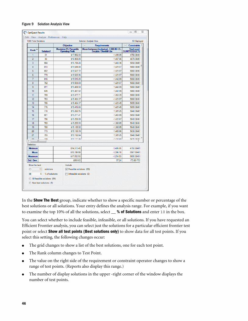
Figure 9 Solution Analysis View
In the Show The Best group, indicate whether to show a specific number or percentage of thebest solutions or all solutions. Your entry defines the analysis range. For example, if you wantto examine the top 10% of all the solutions, select __ % of Solutions and enter 10 in the box.
You can select whether to include feasible, infeasible, or all solutions. If you have requested anEfficient Frontier analysis, you can select just the solutions for a particular efficient frontier testpoint or select Show all test points (Best solutions only) to show data for all test points. If youselect this setting, the following changes occur:
l The grid changes to show a list of the best solutions, one for each test point.
l The Rank column changes to Test Point.
l The value on the right side of the requirement or constraint operator changes to show arange of test points. (Reports also display this range.)
l The number of display solutions in the upper -right corner of the window displays thenumber of test points.
46
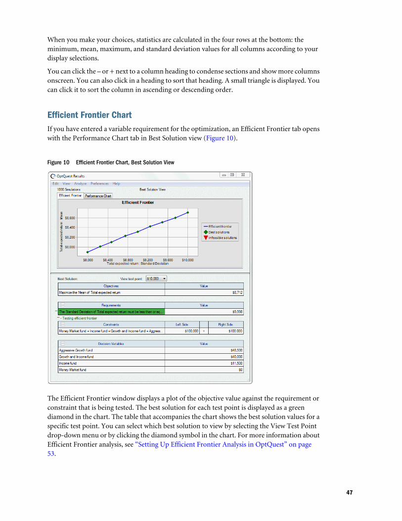
When you make your choices, statistics are calculated in the four rows at the bottom: theminimum, mean, maximum, and standard deviation values for all columns according to yourdisplay selections.
You can click the – or + next to a column heading to condense sections and show more columnsonscreen. You can also click in a heading to sort that heading. A small triangle is displayed. Youcan click it to sort the column in ascending or descending order.
Efficient Frontier ChartIf you have entered a variable requirement for the optimization, an Efficient Frontier tab openswith the Performance Chart tab in Best Solution view (Figure 10).
Figure 10 Efficient Frontier Chart, Best Solution View
The Efficient Frontier window displays a plot of the objective value against the requirement orconstraint that is being tested. The best solution for each test point is displayed as a greendiamond in the chart. The table that accompanies the chart shows the best solution values for aspecific test point. You can select which best solution to view by selecting the View Test Pointdrop-down menu or by clicking the diamond symbol in the chart. For more information aboutEfficient Frontier analysis, see “Setting Up Efficient Frontier Analysis in OptQuest” on page53.
47
Interpreting the ResultsAfter solving an optimization problem with OptQuest, you can do the following:
1. View a solution analysis to determine the robustness of the results.
2. Run a longer Crystal Ball simulation using the optimal values of the decision variables tomore accurately assess the risks of the recommended solution.
3. Use Crystal Ball’s analysis features to further evaluate the optimal solution.
Viewing a Solution Analysis
ä After the optimization is finished, interpret your optimization results:
1 Select View, and then Solution Analysis in the OptQuest Results window.
The Solution Analysis view opens with a partial listing of the solutions that OptQuest triedduring the optimization. The solutions are shown row-wise in the upper grid with a smallergrid giving the statistics for each column.
Notice that the OptQuest Results window has several menus you can use to copy results toyour spreadsheet, copy charts, print results, view other charts, and more. For a list of menucommands and their shortcut keys, see the Oracle Crystal Ball Accessibility Guide.
2 Select which solutions to view.
Along with both grids are groups of controls you can use to filter the solutions to view. Allof the controls combine to filter the set of solutions. Some controls show the number ofsolutions that will be included in parenthesis.
l In the first group, select to view only the top number or percentage of best solutions(highest or lowest objective values), all of the solutions, or only the new best solutions(corresponding to up or down “jumps” in the performance chart).
l In the next group, select whether to include feasible, infeasible, or both types of solutions.
l If you have requested an efficient frontier analysis, select a test point from the dropdownmenu in the last group. Notice that all of the solutions are considered for a particulartest point, even if they were evaluated at a previous or later test point in the optimization.
Once you have chosen a set of solutions to analyze, you can click in a column heading to sortthe solution by that heading. The small triangle indicates the direction of the sort order. Youcan also click the + or – symbol beside a group of columns to condense or expand the amountof information displayed.
Bounds AnalysisThe Solution Analysis view is useful for determining how restrictive the bounds are forrequirements or constraints, especially when there are multiple bounds involved. When viewingthe best solutions for an optimization, if most of the values for a requirement or constraint are
48
at or near a specific bound, this indicates that the requirement or constraint is having a significanteffect on the values that are obtainable for the objective.
Sensitivity AnalysisThe Solution Analysis view is useful for determining the sensitivity of decision variables withrespect to the model’s objective. When viewing the best solutions for an optimization, comparethe relative size of the ranges for each of your decision variables. Generally speaking, a decisionvariable with a smaller relative range indicates that it has a greater impact on the objective. Thisis because small changes in the decision variable can force the solutions to be less than optimal.Conversely, a decision variable with a wider relative range indicates that is has a lesser impacton the objective since different values do not seem to alter the set of best solutions.
These are general guidelines only. The results for your situation can be affected by the type andlength of the optimization, the initial bounds defined for the decision variables, and other factors.
Running a Longer Simulation of the Results
ä To more accurately assess the recommended solution, run a longer Crystal Ball simulationusing the optimal values of the decision variables.
1 If you did not select to automatically copy OptQuest results to the model workbook (set in theOptions panel), you can select Edit, and then Copy Solution to Spreadsheet in the OptQuest Resultswindow.
OptQuest copies the decision variables values from the selected solution into the MicrosoftExcel model.
2 In Crystal Ball, reset the optimization, click the Run Preferences button, and increase the maximumnumber of trials per simulation.
3 Run the simulation.
4 Use Crystal Ball analysis tools to analyze your results.
For more information on using these tools, see the Oracle Crystal Ball User's Guide.
Printing OptQuest Results
ä To print results from any OptQuest results view:
1 Run an OptQuest optimization and open the OptQuest Results window.
2 Select a view from the View menu in the OptQuest Results window menu bar.
3 Select Edit in the OptQuest Results window menu bar.
4 Select an appropriate command related to printing at the bottom of the Edit menu: Page Setup, PrintPreview, and Print.
49
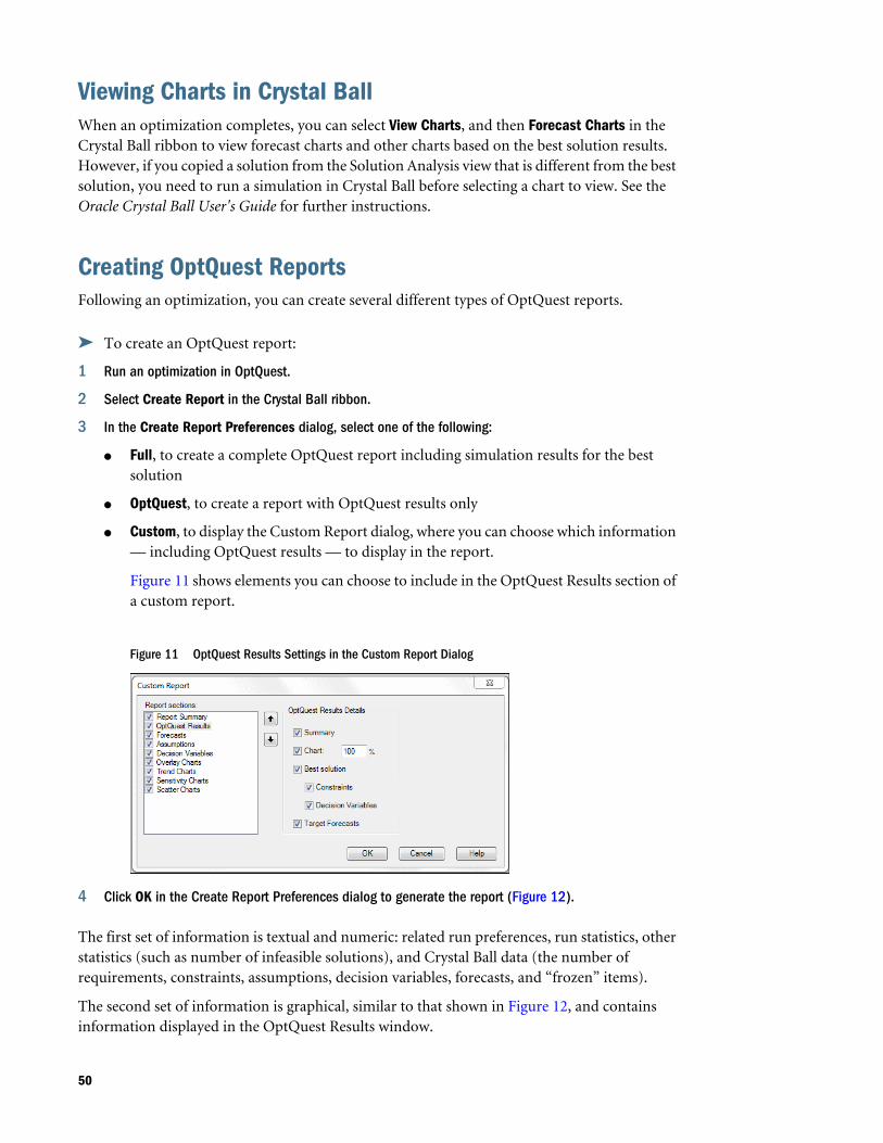
Viewing Charts in Crystal BallWhen an optimization completes, you can select View Charts, and then Forecast Charts in theCrystal Ball ribbon to view forecast charts and other charts based on the best solution results.However, if you copied a solution from the Solution Analysis view that is different from the bestsolution, you need to run a simulation in Crystal Ball before selecting a chart to view. See theOracle Crystal Ball User's Guide for further instructions.
Creating OptQuest ReportsFollowing an optimization, you can create several different types of OptQuest reports.
ä To create an OptQuest report:
1 Run an optimization in OptQuest.
2 Select Create Report in the Crystal Ball ribbon.
3 In the Create Report Preferences dialog, select one of the following:
l Full, to create a complete OptQuest report including simulation results for the bestsolution
l OptQuest, to create a report with OptQuest results only
l Custom, to display the Custom Report dialog, where you can choose which information— including OptQuest results — to display in the report.
Figure 11 shows elements you can choose to include in the OptQuest Results section ofa custom report.
Figure 11 OptQuest Results Settings in the Custom Report Dialog
4 Click OK in the Create Report Preferences dialog to generate the report (Figure 12).
The first set of information is textual and numeric: related run preferences, run statistics, otherstatistics (such as number of infeasible solutions), and Crystal Ball data (the number ofrequirements, constraints, assumptions, decision variables, forecasts, and “frozen” items).
The second set of information is graphical, similar to that shown in Figure 12, and containsinformation displayed in the OptQuest Results window.
50
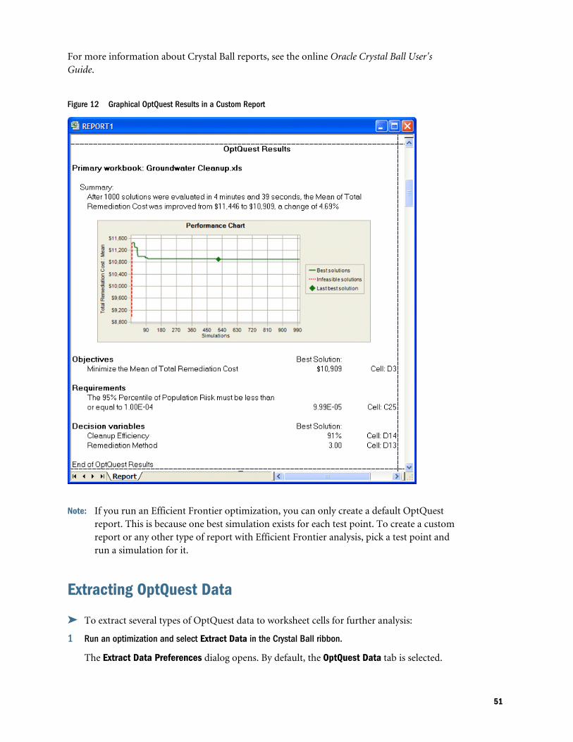
For more information about Crystal Ball reports, see the online Oracle Crystal Ball User'sGuide.
Figure 12 Graphical OptQuest Results in a Custom Report
Note: If you run an Efficient Frontier optimization, you can only create a default OptQuestreport. This is because one best simulation exists for each test point. To create a customreport or any other type of report with Efficient Frontier analysis, pick a test point andrun a simulation for it.
Extracting OptQuest Data
ä To extract several types of OptQuest data to worksheet cells for further analysis:
1 Run an optimization and select Extract Data in the Crystal Ball ribbon.
The Extract Data Preferences dialog opens. By default, the OptQuest Data tab is selected.
51
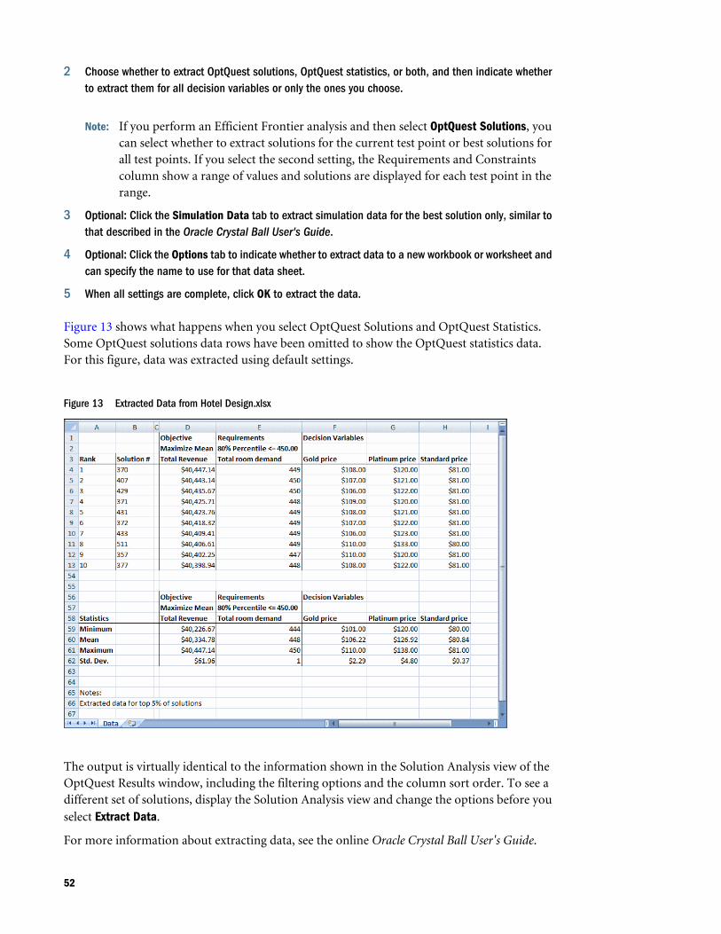
2 Choose whether to extract OptQuest solutions, OptQuest statistics, or both, and then indicate whetherto extract them for all decision variables or only the ones you choose.
Note: If you perform an Efficient Frontier analysis and then select OptQuest Solutions, youcan select whether to extract solutions for the current test point or best solutions forall test points. If you select the second setting, the Requirements and Constraintscolumn show a range of values and solutions are displayed for each test point in therange.
3 Optional: Click the Simulation Data tab to extract simulation data for the best solution only, similar tothat described in the Oracle Crystal Ball User's Guide.
4 Optional: Click the Options tab to indicate whether to extract data to a new workbook or worksheet andcan specify the name to use for that data sheet.
5 When all settings are complete, click OK to extract the data.
Figure 13 shows what happens when you select OptQuest Solutions and OptQuest Statistics.Some OptQuest solutions data rows have been omitted to show the OptQuest statistics data.For this figure, data was extracted using default settings.
Figure 13 Extracted Data from Hotel Design.xlsx
The output is virtually identical to the information shown in the Solution Analysis view of theOptQuest Results window, including the filtering options and the column sort order. To see adifferent set of solutions, display the Solution Analysis view and change the options before youselect Extract Data.
For more information about extracting data, see the online Oracle Crystal Ball User's Guide.
52
Saving Optimization Models and SettingsWhen you run an optimization, current settings on the Options panel and Advanced Optionsdialog are automatically saved in a preference file and will be applied to future optimizations.
Other settings — such as objectives, requirements, and constraint definitions — are saved inthe primary workbook selected in the dropdown list on the Objectives panel. They are saved tothe workbook when the optimization runs, however they are not saved permanently until yousave the primary workbook itself.
If you choose to copy optimization values to the model, these values are displayed as the newcell values and are also saved when the model is saved. Each workbook can have one set ofoptimization settings.
If you click Close in the OptQuest wizard before you run an optimization, OptQuest asks whetherto save the settings. If you respond Yes, current settings are saved to the workbook. Otherwise,current settings are discarded and the last saved settings remain.
Closing OptQuestTo exit OptQuest without running an optimization, click Close in the OptQuest wizard.
If you have not saved changes to the optimization settings yet, OptQuest prompts you to savethem to the primary workbook.
Setting Up Efficient Frontier Analysis in OptQuestEfficient Frontier analysis calculates the curve that plots an objective value against changes to arequirement or constraint. A typical use is for comparing portfolio returns against different risklevels so that investors can maximize return and minimize risk. For a theoretical discussion, see“Efficient Frontier Analysis” on page 21. For an illustration of an Efficient Frontier chart, seeFigure 10. For an example, see the Oracle Crystal Ball Reference and Examples Guide.
To request an Efficient Frontier analysis in OptQuest, you need to define a requirement or aconstraint with a variable bound in either the Objectives or Constraints panel of the OptQuestwizard.
ä To define a variable bound for Efficient Frontier analysis:
1 In the Objectives panel, select an existing requirement to modify or add a new one and select it.
Alternately, select a constraint in the Constraints panel.
2 Click Efficient Frontier.
3 An Efficient Frontier row opens near the requirement or constraint. Adjust the underlined elements todefine a range of values for one or both bounds of the requirement or constraint.
When you define a range for a requirement or constraint bound (instead of a single point), youalso define a number of points to check within the range by setting the step amount. OptQuest
53
runs one full optimization for each test point in the range, starting with the most limitingrequirement test point. Then, you can see the effects of tightening or loosening a requirement.
Efficient Frontier Variable Bound ExampleIn “Tutorial 2 — Portfolio Allocation Model ” on page 63, the investor wants to impose acondition that limits the standard deviation of the total return. Because the standard deviationis a forecast statistic and not a decision variable, this restriction is a requirement.
However, if the investor wants to see if a small increase in the requirement could create a sharpincrease in the investment return, the investor can set this as a requirement with a variable upperbound (since this limits the maximum standard deviation). The investor can define this upperbound with a lower limit of $8,000 and an upper limit of $10,000. For an example of thistechnique, see Portfolio Revisited EF.xlsx.
Transferring Settings from .opt FilesOptQuest versions shipped with previous releases of Crystal Ball (prior to 11.1.1.x) storedoptimization settings in .opt files. As described in “Saving Optimization Models and Settings”on page 53, this version of OptQuest saves settings in workbooks. An .opt file viewer is availableto help you transfer settings from .opt files into this version.
ä To use the .opt file viewer:
1 Open an optimization model created in a version of Crystal Ball earlier than 11.1.1. The model shouldhave at least one forecast and one decision variable defined. They can be “dummy” data cells, and youcan delete them later if you need to.
2 Select OptQuest, .
3 When the Objectives panel opens, click Import.
The Import Optimization Settings dialog opens.
4 Click Browse to locate the .opt file. When you reach its folder, double-click the file. Its settings aredisplayed in the Import Optimization Settings dialog (Figure 14, following).
54
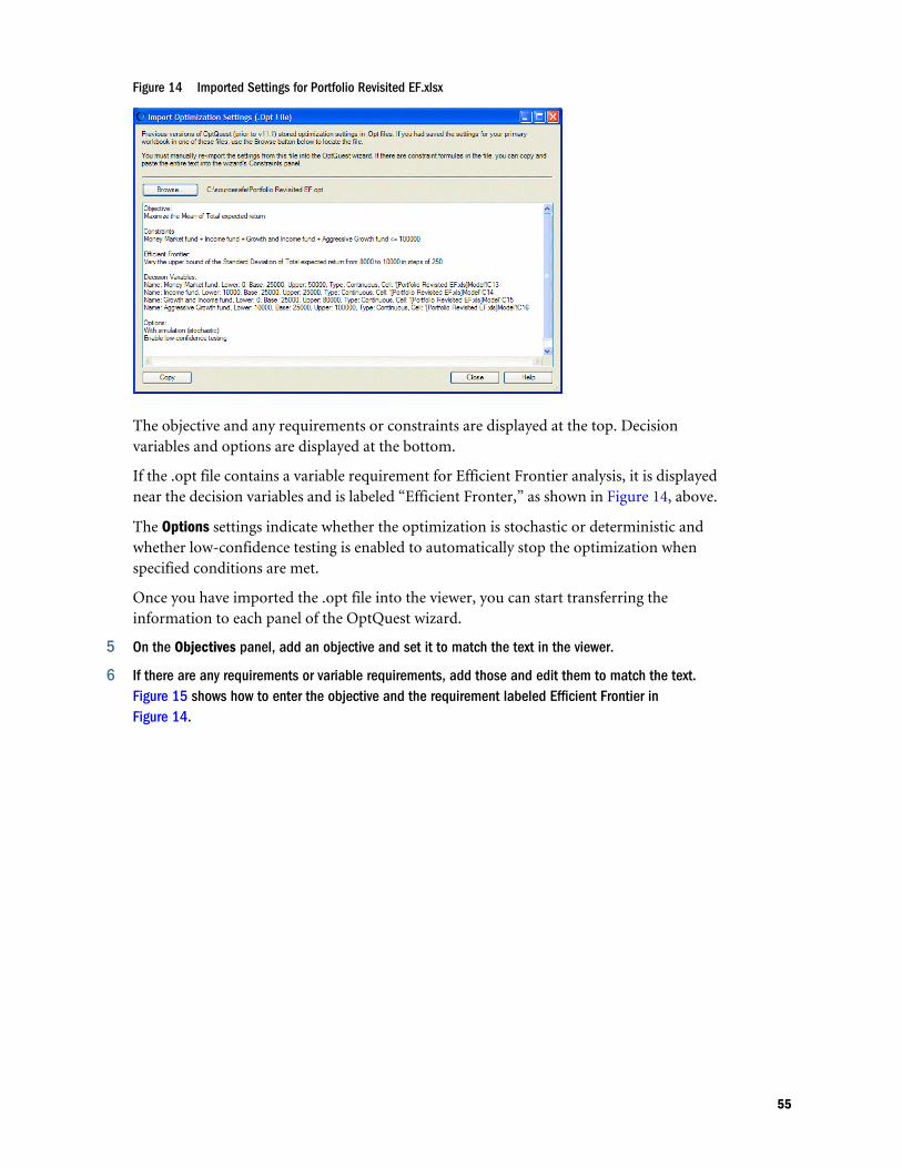
Figure 14 Imported Settings for Portfolio Revisited EF.xlsx
The objective and any requirements or constraints are displayed at the top. Decisionvariables and options are displayed at the bottom.
If the .opt file contains a variable requirement for Efficient Frontier analysis, it is displayednear the decision variables and is labeled “Efficient Fronter,” as shown in Figure 14, above.
The Options settings indicate whether the optimization is stochastic or deterministic andwhether low-confidence testing is enabled to automatically stop the optimization whenspecified conditions are met.
Once you have imported the .opt file into the viewer, you can start transferring theinformation to each panel of the OptQuest wizard.
5 On the Objectives panel, add an objective and set it to match the text in the viewer.
6 If there are any requirements or variable requirements, add those and edit them to match the text.Figure 15 shows how to enter the objective and the requirement labeled Efficient Frontier inFigure 14.
55
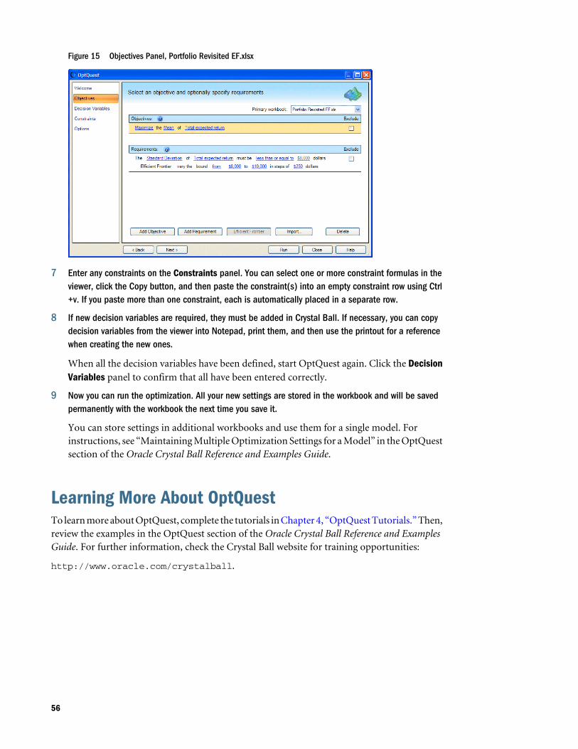
Figure 15 Objectives Panel, Portfolio Revisited EF.xlsx
7 Enter any constraints on the Constraints panel. You can select one or more constraint formulas in theviewer, click the Copy button, and then paste the constraint(s) into an empty constraint row using Ctrl+v. If you paste more than one constraint, each is automatically placed in a separate row.
8 If new decision variables are required, they must be added in Crystal Ball. If necessary, you can copydecision variables from the viewer into Notepad, print them, and then use the printout for a referencewhen creating the new ones.
When all the decision variables have been defined, start OptQuest again. Click the DecisionVariables panel to confirm that all have been entered correctly.
9 Now you can run the optimization. All your new settings are stored in the workbook and will be savedpermanently with the workbook the next time you save it.
You can store settings in additional workbooks and use them for a single model. Forinstructions, see “Maintaining Multiple Optimization Settings for a Model” in the OptQuestsection of the Oracle Crystal Ball Reference and Examples Guide.
Learning More About OptQuestTo learn more about OptQuest, complete the tutorials in Chapter 4, “OptQuest Tutorials.” Then,review the examples in the OptQuest section of the Oracle Crystal Ball Reference and ExamplesGuide. For further information, check the Crystal Ball website for training opportunities:
http://www.oracle.com/crystalball.
56
4OptQuest Tutorials
In This Chapter
Introduction... . . . . . . . . . . . . . . . . . . . . . . . . . . . . . . . . . . . . . . . . . . . . . . . . . . . . . . . . . . . . . . . . . . . . . . . . . . . . . . . . . . . . . . . . . . . . . .57
Tutorial 1 — Futura Apartments Model .. . . . . . . . . . . . . . . . . . . . . . . . . . . . . . . . . . . . . . . . . . . . . . . . . . . . . . . . . . . . . . . . . .57
Tutorial 2 — Portfolio Allocation Model . . . . . . . . . . . . . . . . . . . . . . . . . . . . . . . . . . . . . . . . . . . . . . . . . . . . . . . . . . . . . . . . . .63
IntroductionThe first tutorial, the Futura Apartments model, is an extension of the model used in the firstCrystal Ball tutorial in the Oracle Crystal Ball User's Guide and finds the optimal rent for anapartment building. This model is virtually ready to run, so you can quickly see how OptQuestworks.
The second tutorial, the Portfolio Allocation model, shows how to set up and define anoptimization yourself. This model finds the optimal set of investments that balances the risk andthe return of an investment portfolio.
Tutorial 1 — Futura Apartments ModelSuppose that you have recently purchased the Futura Apartments complex. One of your criticaldecisions is the amount of rent to charge. You have researched the situation and created aspreadsheet model to help you make a knowledgeable decision.
From the analysis of the price structures and occupancy rates of similar apartment complexes,you have estimated that demand for rental units is a linear function of the rent charged, and isexpressed as:
Number of units rented = -.1(rent per unit) + 85
for rents between $400 and $600.
In addition, you have estimated that operating costs will average about $15,000 per month forthe entire complex.
Note: You can use Predictor, supplied with Crystal Ball, to find the linear relationship of adependent variable to one or more independent variables.
57
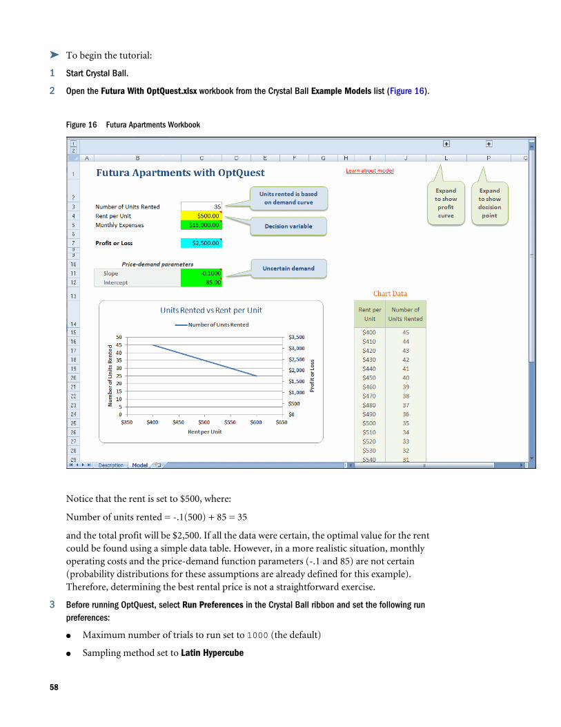
ä To begin the tutorial:
1 Start Crystal Ball.
2 Open the Futura With OptQuest.xlsx workbook from the Crystal Ball Example Models list (Figure 16).
Figure 16 Futura Apartments Workbook
Notice that the rent is set to $500, where:
Number of units rented = -.1(500) + 85 = 35
and the total profit will be $2,500. If all the data were certain, the optimal value for the rentcould be found using a simple data table. However, in a more realistic situation, monthlyoperating costs and the price-demand function parameters (-.1 and 85) are not certain(probability distributions for these assumptions are already defined for this example).Therefore, determining the best rental price is not a straightforward exercise.
3 Before running OptQuest, select Run Preferences in the Crystal Ball ribbon and set the following runpreferences:
l Maximum number of trials to run set to 1000 (the default)
l Sampling method set to Latin Hypercube
58
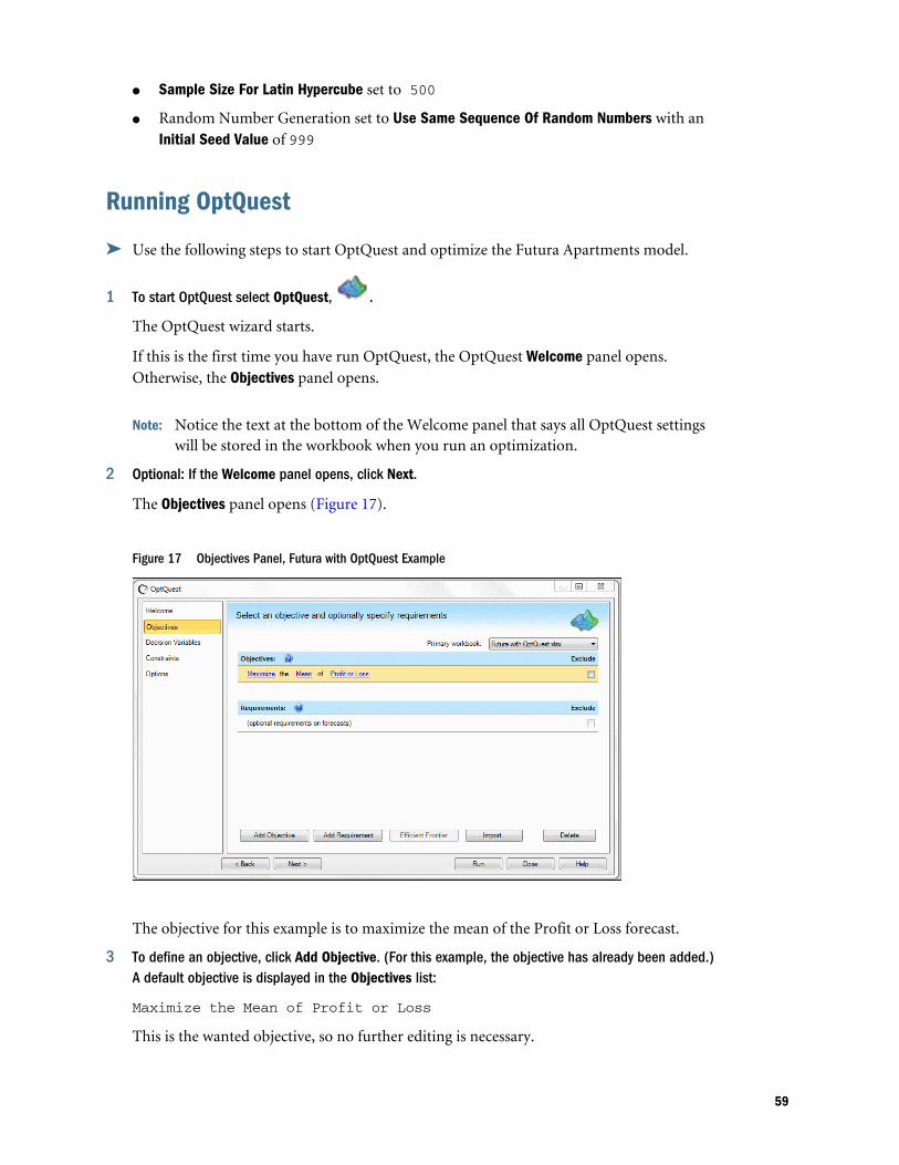
l Sample Size For Latin Hypercube set to 500
l Random Number Generation set to Use Same Sequence Of Random Numbers with anInitial Seed Value of 999
Running OptQuest
ä Use the following steps to start OptQuest and optimize the Futura Apartments model.
1 To start OptQuest select OptQuest, .
The OptQuest wizard starts.
If this is the first time you have run OptQuest, the OptQuest Welcome panel opens.Otherwise, the Objectives panel opens.
Note: Notice the text at the bottom of the Welcome panel that says all OptQuest settingswill be stored in the workbook when you run an optimization.
2 Optional: If the Welcome panel opens, click Next.
The Objectives panel opens (Figure 17).
Figure 17 Objectives Panel, Futura with OptQuest Example
The objective for this example is to maximize the mean of the Profit or Loss forecast.
3 To define an objective, click Add Objective. (For this example, the objective has already been added.)A default objective is displayed in the Objectives list:
Maximize the Mean of Profit or Loss
This is the wanted objective, so no further editing is necessary.
59
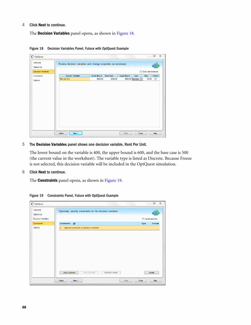
4 Click Next to continue.
The Decision Variables panel opens, as shown in Figure 18.
Figure 18 Decision Variables Panel, Futura with OptQuest Example
5 The Decision Variables panel shows one decision variable, Rent Per Unit.
The lower bound on the variable is 400, the upper bound is 600, and the base case is 500(the current value in the worksheet). The variable type is listed as Discrete. Because Freezeis not selected, this decision variable will be included in the OptQuest simulation.
6 Click Next to continue.
The Constraints panel opens, as shown in Figure 19.
Figure 19 Constraints Panel, Futura with OptQuest Example
60
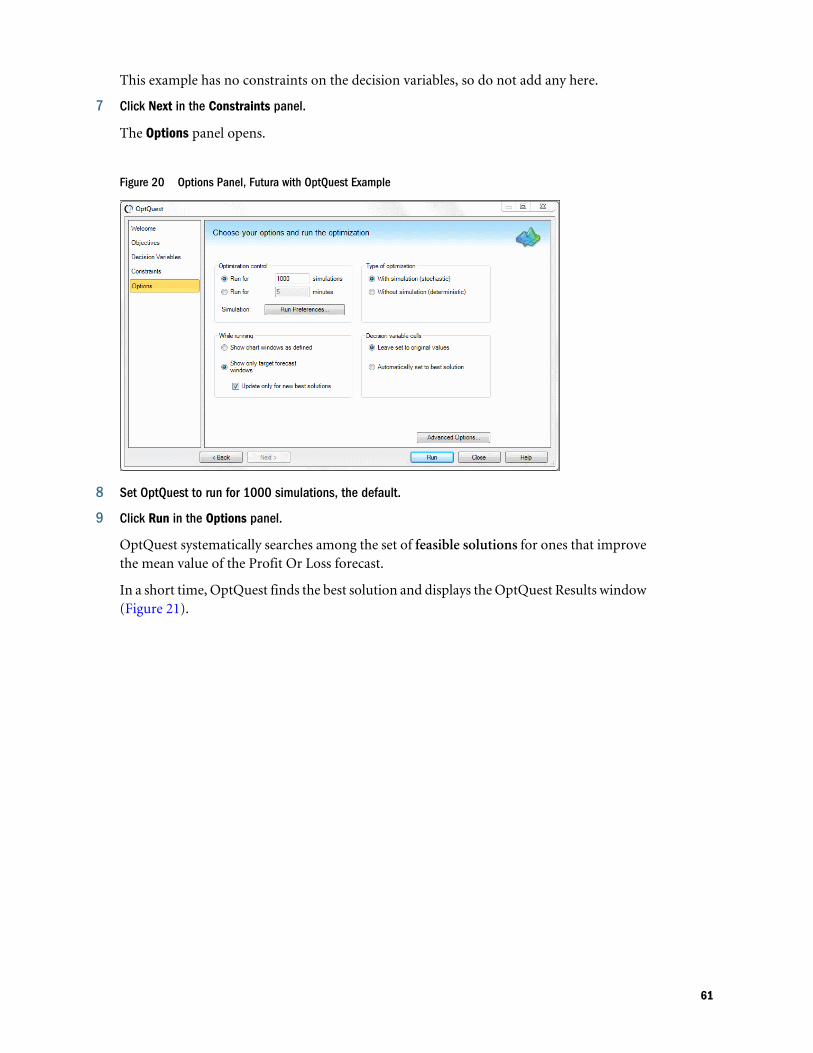
This example has no constraints on the decision variables, so do not add any here.
7 Click Next in the Constraints panel.
The Options panel opens.
Figure 20 Options Panel, Futura with OptQuest Example
8 Set OptQuest to run for 1000 simulations, the default.
9 Click Run in the Options panel.
OptQuest systematically searches among the set of feasible solutions for ones that improvethe mean value of the Profit Or Loss forecast.
In a short time, OptQuest finds the best solution and displays the OptQuest Results window(Figure 21).
61
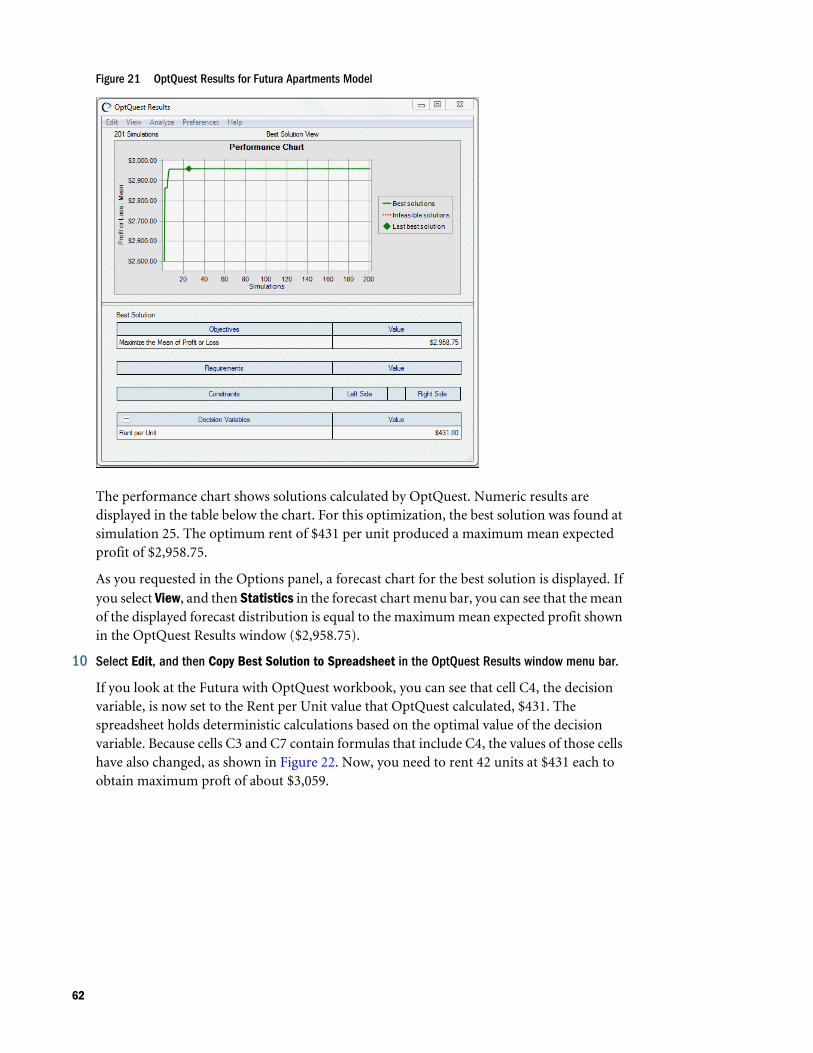
Figure 21 OptQuest Results for Futura Apartments Model
The performance chart shows solutions calculated by OptQuest. Numeric results aredisplayed in the table below the chart. For this optimization, the best solution was found atsimulation 25. The optimum rent of $431 per unit produced a maximum mean expectedprofit of $2,958.75.
As you requested in the Options panel, a forecast chart for the best solution is displayed. Ifyou select View, and then Statistics in the forecast chart menu bar, you can see that the meanof the displayed forecast distribution is equal to the maximum mean expected profit shownin the OptQuest Results window ($2,958.75).
10 Select Edit, and then Copy Best Solution to Spreadsheet in the OptQuest Results window menu bar.
If you look at the Futura with OptQuest workbook, you can see that cell C4, the decisionvariable, is now set to the Rent per Unit value that OptQuest calculated, $431. Thespreadsheet holds deterministic calculations based on the optimal value of the decisionvariable. Because cells C3 and C7 contain formulas that include C4, the values of those cellshave also changed, as shown in Figure 22. Now, you need to rent 42 units at $431 each toobtain maximum proft of about $3,059.
62
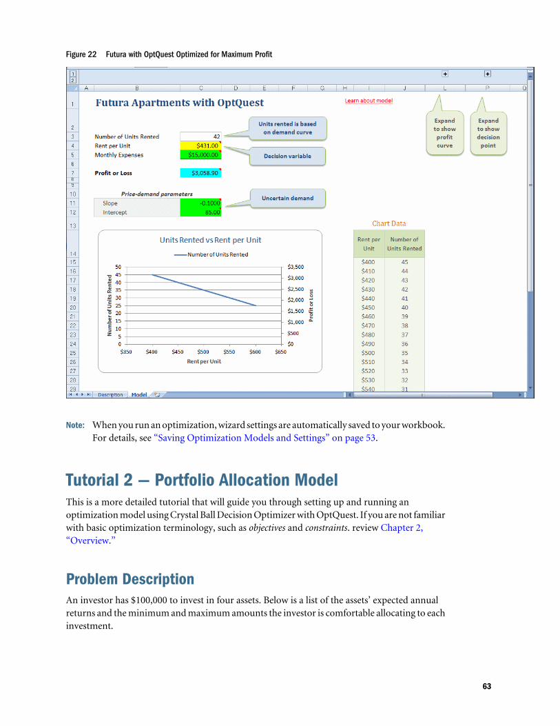
Figure 22 Futura with OptQuest Optimized for Maximum Profit
Note: When you run an optimization, wizard settings are automatically saved to your workbook.For details, see “Saving Optimization Models and Settings” on page 53.
Tutorial 2 — Portfolio Allocation Model This is a more detailed tutorial that will guide you through setting up and running anoptimization model using Crystal Ball Decision Optimizer with OptQuest. If you are not familiarwith basic optimization terminology, such as objectives and constraints. review Chapter 2,“Overview.”
Problem DescriptionAn investor has $100,000 to invest in four assets. Below is a list of the assets’ expected annualreturns and the minimum and maximum amounts the investor is comfortable allocating to eachinvestment.
63
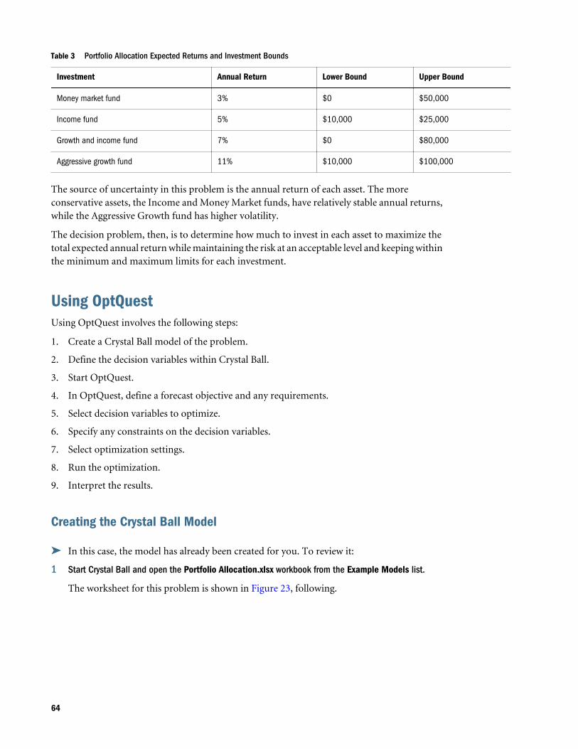
Table 3 Portfolio Allocation Expected Returns and Investment Bounds
Investment Annual Return Lower Bound Upper Bound
Money market fund 3% $0 $50,000
Income fund 5% $10,000 $25,000
Growth and income fund 7% $0 $80,000
Aggressive growth fund 11% $10,000 $100,000
The source of uncertainty in this problem is the annual return of each asset. The moreconservative assets, the Income and Money Market funds, have relatively stable annual returns,while the Aggressive Growth fund has higher volatility.
The decision problem, then, is to determine how much to invest in each asset to maximize thetotal expected annual return while maintaining the risk at an acceptable level and keeping withinthe minimum and maximum limits for each investment.
Using OptQuestUsing OptQuest involves the following steps:
1. Create a Crystal Ball model of the problem.
2. Define the decision variables within Crystal Ball.
3. Start OptQuest.
4. In OptQuest, define a forecast objective and any requirements.
5. Select decision variables to optimize.
6. Specify any constraints on the decision variables.
7. Select optimization settings.
8. Run the optimization.
9. Interpret the results.
Creating the Crystal Ball Model
ä In this case, the model has already been created for you. To review it:
1 Start Crystal Ball and open the Portfolio Allocation.xlsx workbook from the Example Models list.
The worksheet for this problem is shown in Figure 23, following.
64
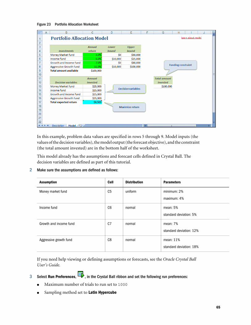
Figure 23 Portfolio Allocation Worksheet
In this example, problem data values are specified in rows 5 through 9. Model inputs (thevalues of the decision variables), the model output (the forecast objective), and the constraint(the total amount invested) are in the bottom half of the worksheet.
This model already has the assumptions and forecast cells defined in Crystal Ball. Thedecision variables are defined as part of this tutorial.
2 Make sure the assumptions are defined as follows:
Assumption Cell Distribution Parameters
Money market fund C5 uniform minimum: 2%
maximum: 4%
Income fund C6 normal mean: 5%
standard deviation: 5%
Growth and income fund C7 normal mean: 7%
standard deviation: 12%
Aggressive growth fund C8 normal mean: 11%
standard deviation: 18%
If you need help viewing or defining assumptions or forecasts, see the Oracle Crystal BallUser's Guide.
3 Select Run Preferences, , in the Crystal Ball ribbon and set the following run preferences:
l Maximum number of trials to run set to 1000
l Sampling method set to Latin Hypercube
65
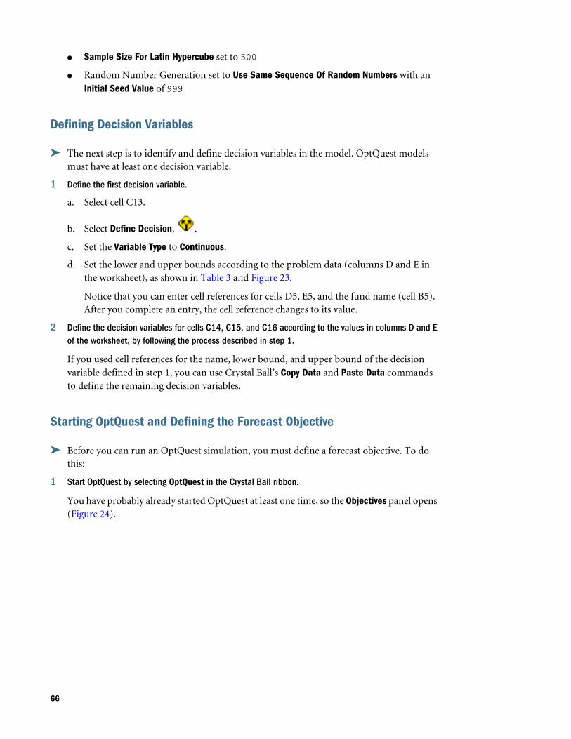
l Sample Size For Latin Hypercube set to 500
l Random Number Generation set to Use Same Sequence Of Random Numbers with anInitial Seed Value of 999
Defining Decision Variables
ä The next step is to identify and define decision variables in the model. OptQuest modelsmust have at least one decision variable.
1 Define the first decision variable.
a. Select cell C13.
b. Select Define Decision, .
c. Set the Variable Type to Continuous.
d. Set the lower and upper bounds according to the problem data (columns D and E inthe worksheet), as shown in Table 3 and Figure 23.
Notice that you can enter cell references for cells D5, E5, and the fund name (cell B5).After you complete an entry, the cell reference changes to its value.
2 Define the decision variables for cells C14, C15, and C16 according to the values in columns D and Eof the worksheet, by following the process described in step 1.
If you used cell references for the name, lower bound, and upper bound of the decisionvariable defined in step 1, you can use Crystal Ball’s Copy Data and Paste Data commandsto define the remaining decision variables.
Starting OptQuest and Defining the Forecast Objective
ä Before you can run an OptQuest simulation, you must define a forecast objective. To dothis:
1 Start OptQuest by selecting OptQuest in the Crystal Ball ribbon.
You have probably already started OptQuest at least one time, so the Objectives panel opens(Figure 24).
66
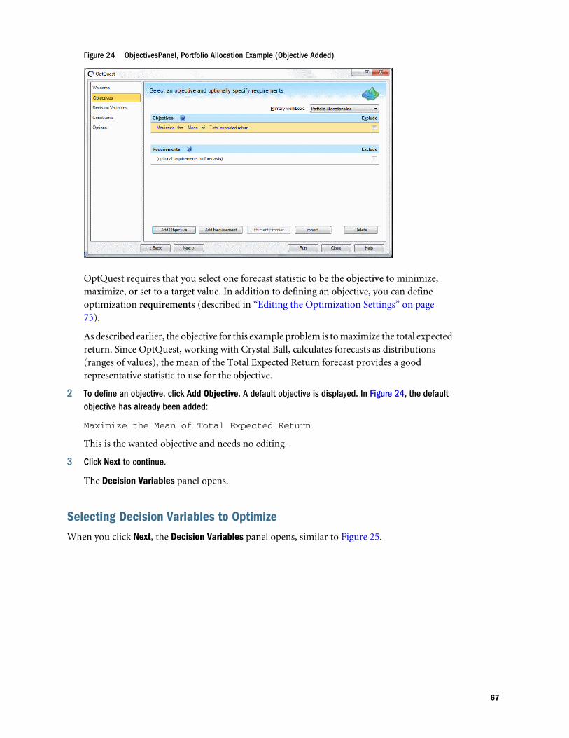
Figure 24 ObjectivesPanel, Portfolio Allocation Example (Objective Added)
OptQuest requires that you select one forecast statistic to be the objective to minimize,maximize, or set to a target value. In addition to defining an objective, you can defineoptimization requirements (described in “Editing the Optimization Settings” on page73).
As described earlier, the objective for this example problem is to maximize the total expectedreturn. Since OptQuest, working with Crystal Ball, calculates forecasts as distributions(ranges of values), the mean of the Total Expected Return forecast provides a goodrepresentative statistic to use for the objective.
2 To define an objective, click Add Objective. A default objective is displayed. In Figure 24, the defaultobjective has already been added:
Maximize the Mean of Total Expected Return
This is the wanted objective and needs no editing.
3 Click Next to continue.
The Decision Variables panel opens.
Selecting Decision Variables to OptimizeWhen you click Next, the Decision Variables panel opens, similar to Figure 25.
67
Figure 25 Decision Variables Panel with Cell Locations, Portfolio Allocation Example
Every decision variable defined in the Crystal Ball model is displayed in the Decision Variablespanel. The last column indicates whether the variable has been “frozen,” or removed from theoptimization. In Figure 25, Show cell locations is selected so cell addresses are displayed beforethe last column.
The other columns show the bounds, base case (current model value), type, and step for eachvariable.
ä The settings are correct for this example, so select Show cell locations and click Next tocontinue.
The Constraints panel opens, as shown in Figure 26.
Specifying ConstraintsWhen you click Next in the Decision Variables panel, the Constraints panel opens.
68
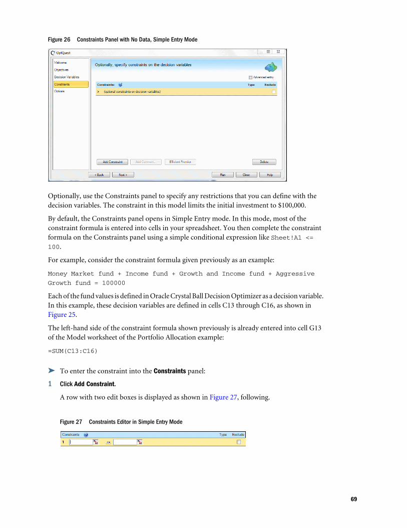
Figure 26 Constraints Panel with No Data, Simple Entry Mode
Optionally, use the Constraints panel to specify any restrictions that you can define with thedecision variables. The constraint in this model limits the initial investment to $100,000.
By default, the Constraints panel opens in Simple Entry mode. In this mode, most of theconstraint formula is entered into cells in your spreadsheet. You then complete the constraintformula on the Constraints panel using a simple conditional expression like Sheet!A1 <=100.
For example, consider the constraint formula given previously as an example:
Money Market fund + Income fund + Growth and Income fund + Aggressive
Growth fund = 100000
Each of the fund values is defined in Oracle Crystal Ball Decision Optimizer as a decision variable.In this example, these decision variables are defined in cells C13 through C16, as shown inFigure 25.
The left-hand side of the constraint formula shown previously is already entered into cell G13of the Model worksheet of the Portfolio Allocation example:
=SUM(C13:C16)
ä To enter the constraint into the Constraints panel:
1 Click Add Constraint.
A row with two edit boxes is displayed as shown in Figure 27, following.
Figure 27 Constraints Editor in Simple Entry Mode
69
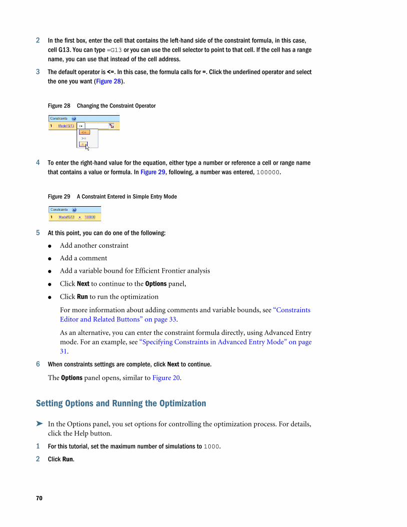
2 In the first box, enter the cell that contains the left-hand side of the constraint formula, in this case,cell G13. You can type =G13 or you can use the cell selector to point to that cell. If the cell has a rangename, you can use that instead of the cell address.
3 The default operator is <=. In this case, the formula calls for =. Click the underlined operator and selectthe one you want (Figure 28).
Figure 28 Changing the Constraint Operator
4 To enter the right-hand value for the equation, either type a number or reference a cell or range namethat contains a value or formula. In Figure 29, following, a number was entered, 100000.
Figure 29 A Constraint Entered in Simple Entry Mode
5 At this point, you can do one of the following:
l Add another constraint
l Add a comment
l Add a variable bound for Efficient Frontier analysis
l Click Next to continue to the Options panel,
l Click Run to run the optimization
For more information about adding comments and variable bounds, see “ConstraintsEditor and Related Buttons” on page 33.
As an alternative, you can enter the constraint formula directly, using Advanced Entrymode. For an example, see “Specifying Constraints in Advanced Entry Mode” on page31.
6 When constraints settings are complete, click Next to continue.
The Options panel opens, similar to Figure 20.
Setting Options and Running the Optimization
ä In the Options panel, you set options for controlling the optimization process. For details,click the Help button.
1 For this tutorial, set the maximum number of simulations to 1000.
2 Click Run.
70
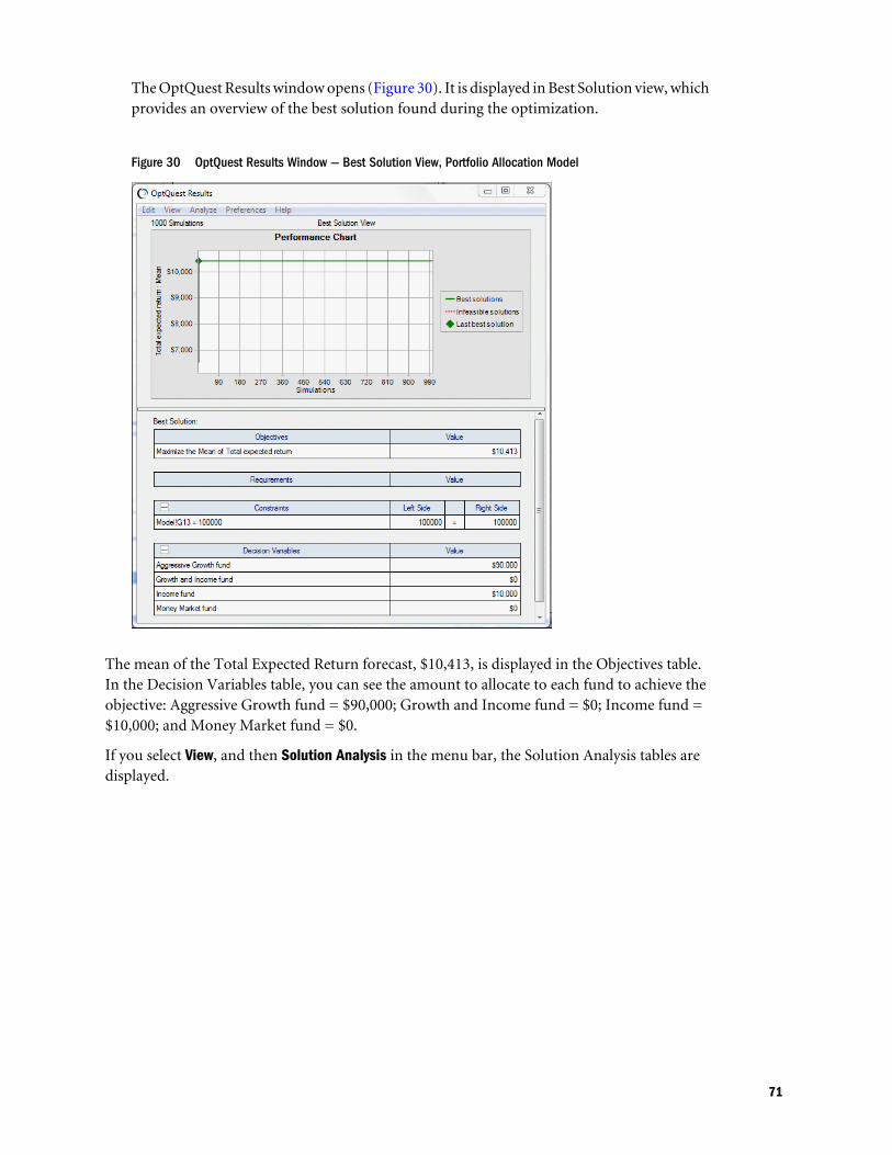
The OptQuest Results window opens (Figure 30). It is displayed in Best Solution view, whichprovides an overview of the best solution found during the optimization.
Figure 30 OptQuest Results Window — Best Solution View, Portfolio Allocation Model
The mean of the Total Expected Return forecast, $10,413, is displayed in the Objectives table.In the Decision Variables table, you can see the amount to allocate to each fund to achieve theobjective: Aggressive Growth fund = $90,000; Growth and Income fund = $0; Income fund =$10,000; and Money Market fund = $0.
If you select View, and then Solution Analysis in the menu bar, the Solution Analysis tables aredisplayed.
71
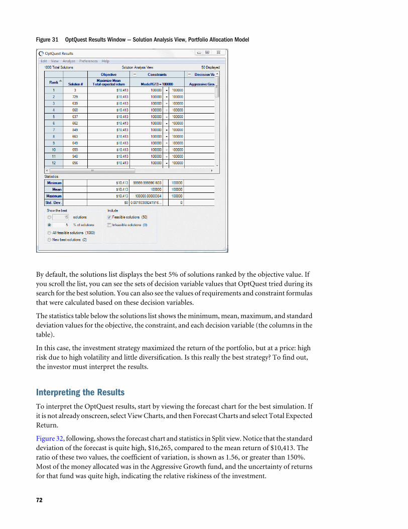
Figure 31 OptQuest Results Window — Solution Analysis View, Portfolio Allocation Model
By default, the solutions list displays the best 5% of solutions ranked by the objective value. Ifyou scroll the list, you can see the sets of decision variable values that OptQuest tried during itssearch for the best solution. You can also see the values of requirements and constraint formulasthat were calculated based on these decision variables.
The statistics table below the solutions list shows the minimum, mean, maximum, and standarddeviation values for the objective, the constraint, and each decision variable (the columns in thetable).
In this case, the investment strategy maximized the return of the portfolio, but at a price: highrisk due to high volatility and little diversification. Is this really the best strategy? To find out,the investor must interpret the results.
Interpreting the ResultsTo interpret the OptQuest results, start by viewing the forecast chart for the best simulation. Ifit is not already onscreen, select View Charts, and then Forecast Charts and select Total ExpectedReturn.
Figure 32, following, shows the forecast chart and statistics in Split view. Notice that the standarddeviation of the forecast is quite high, $16,265, compared to the mean return of $10,413. Theratio of these two values, the coefficient of variation, is shown as 1.56, or greater than 150%.Most of the money allocated was in the Aggressive Growth fund, and the uncertainty of returnsfor that fund was quite high, indicating the relative riskiness of the investment.
72
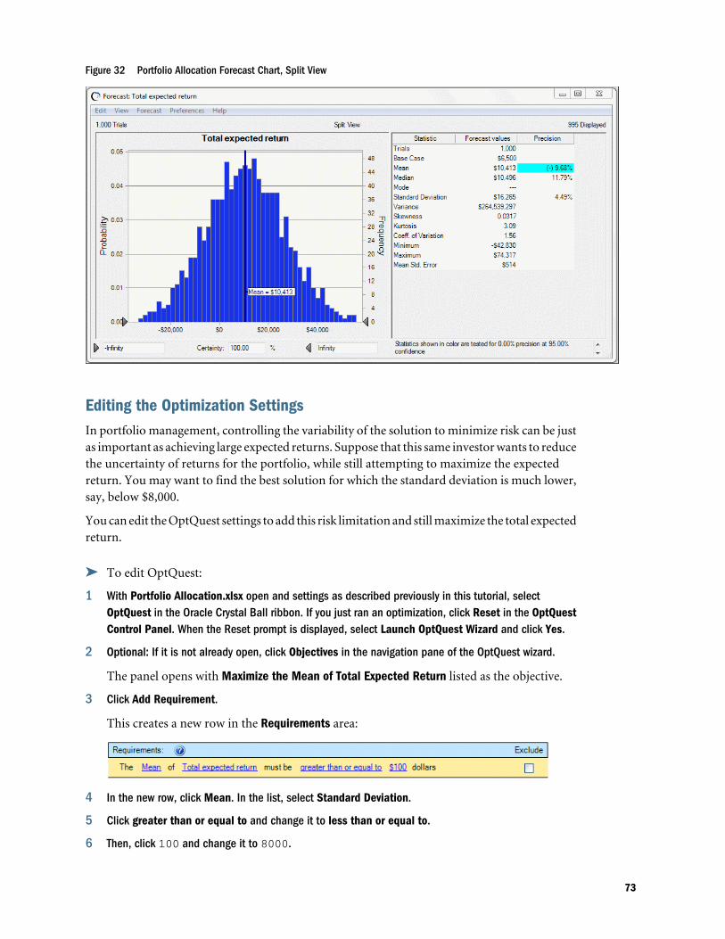
Figure 32 Portfolio Allocation Forecast Chart, Split View
Editing the Optimization SettingsIn portfolio management, controlling the variability of the solution to minimize risk can be justas important as achieving large expected returns. Suppose that this same investor wants to reducethe uncertainty of returns for the portfolio, while still attempting to maximize the expectedreturn. You may want to find the best solution for which the standard deviation is much lower,say, below $8,000.
You can edit the OptQuest settings to add this risk limitation and still maximize the total expectedreturn.
ä To edit OptQuest:
1 With Portfolio Allocation.xlsx open and settings as described previously in this tutorial, selectOptQuest in the Oracle Crystal Ball ribbon. If you just ran an optimization, click Reset in the OptQuestControl Panel. When the Reset prompt is displayed, select Launch OptQuest Wizard and click Yes.
2 Optional: If it is not already open, click Objectives in the navigation pane of the OptQuest wizard.
The panel opens with Maximize the Mean of Total Expected Return listed as the objective.
3 Click Add Requirement.
This creates a new row in the Requirements area:
4 In the new row, click Mean. In the list, select Standard Deviation.
5 Click greater than or equal to and change it to less than or equal to.
6 Then, click 100 and change it to 8000.
73
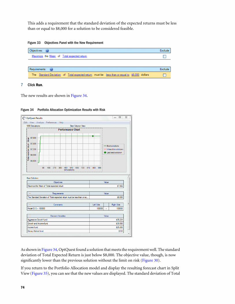
This adds a requirement that the standard deviation of the expected returns must be lessthan or equal to $8,000 for a solution to be considered feasible.
Figure 33 Objectives Panel with the New Requirement
7 Click Run.
The new results are shown in Figure 34.
Figure 34 Portfolio Allocation Optimization Results with Risk
As shown in Figure 34, OptQuest found a solution that meets the requirement well. The standarddeviation of Total Expected Return is just below $8,000. The objective value, though, is nowsignificantly lower than the previous solution without the limit on risk (Figure 30).
If you return to the Portfolio Allocation model and display the resulting forecast chart in SplitView (Figure 35), you can see that the new values are displayed. The standard deviation of Total
74
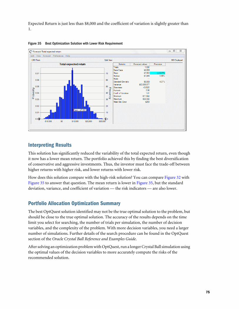
Expected Return is just less than $8,000 and the coefficient of variation is slightly greater than1.
Figure 35 Best Optimization Solution with Lower Risk Requirement
Interpreting ResultsThis solution has significantly reduced the variability of the total expected return, even thoughit now has a lower mean return. The portfolio achieved this by finding the best diversificationof conservative and aggressive investments. Thus, the investor must face the trade-off betweenhigher returns with higher risk, and lower returns with lower risk.
How does this solution compare with the high-risk solution? You can compare Figure 32 withFigure 35 to answer that question. The mean return is lower in Figure 35, but the standarddeviation, variance, and coefficient of variation — the risk indicators — are also lower.
Portfolio Allocation Optimization SummaryThe best OptQuest solution identified may not be the true optimal solution to the problem, butshould be close to the true optimal solution. The accuracy of the results depends on the timelimit you select for searching, the number of trials per simulation, the number of decisionvariables, and the complexity of the problem. With more decision variables, you need a largernumber of simulations. Further details of the search procedure can be found in the OptQuestsection of the Oracle Crystal Ball Reference and Examples Guide.
After solving an optimization problem with OptQuest, run a longer Crystal Ball simulation usingthe optimal values of the decision variables to more accurately compute the risks of therecommended solution.
75

76
Glossary
APT Arbitrage Pricing Theory.
assumption An estimated value or input to a spreadsheet
model. Assumptions capture the uncertainty of model data
using probability distributions.
bound A maximum or minimum limit you set for each
decision variable.
certainty The percentage of simulation results that fall
within a range.
coefficient of variation A measure of relative variation that
compares the standard deviation to the mean. Results can
be represented in percentages for comparison purposes.
constraint A limitation that restricts the possible solutions
to a model. You must define constraints in terms of decision
variables.
continuous A variable that can be fractional (that is, it can
take on any value between the lower and upper bounds). No
step size is required and any given range contains an infinite
number of possible values. Continuous also describes an
optimization model that contains only continuous
variables.
correlation A dependency that exists between assumption
cells.
correlation coefficient A number between -1 and 1 that
specifies mathematically the degree of positive or negative
correlation between assumption cells. A correlation of 1
indicates a perfect positive correlation, minus 1 indicates a
perfect negative correlation, and 0 indicates there is no
correlation.
decision variable A variable in your model that you can
control.
deterministic A model or system with no random variables
that yields single-valued results.
discrete variable A variable that can only assume values equal
to its lower bound plus a multiple of its step size; a step size
is any number greater than zero, but less than the variable’s
range. Discrete also describes an optimization model that
contains only discrete variables.
distribution See probability distribution.
efficient frontier The curve that plots an objective value
against changes to a requirement or constraint. A typical use
is for comparing portfolio returns against different risk
levels.
efficient portfolio Combinations of assets for which it is
impossible to obtain higher returns without generating
higher risk or lower risk without generating lower returns.
An efficient portfolio lies directly on the efficient frontier.
EOQ Economic Order Quantity.
feasible solution A solution that satisfies any constraints
imposed on the decision variables, as well as any
requirements imposed on forecast statistics.
final value The last value that is calculated for a forecast
during a simulation. The final value is useful for when a
forecast contains a function that accumulates values across
the trials of a simulation, or is a function that calculates the
statistic of another forecast.
forecast A statistical summary of the mathematical
combination of the assumptions in a spreadsheet model,
output graphically or numerically. Forecasts are frequency
distributions of possible results for the model.
forecast objective One forecast from a model that OptQuest
uses as the primary goal of the optimization. OptQuest
maximizes or minimizes a statistic of the forecast’s
distribution.
77
forecast statistic Summary values of a forecast distribution,
such as the mean, standard deviation, or variance. You
control the optimization by maximizing or minimizing
forecast statistics or setting them to a target value.
frequency distribution A chart that graphically summarizes a
list of values by sub-dividing them into groups and
displaying their frequency counts.
heuristic An approximate and self-educating technique for
improving solutions.
inventory Any resource set aside for future use, such as raw
materials, semifinished products, and finished products.
Inventory also includes human, financial, and other
resources.
inventory level The amount of inventory on hand, not
counting ordered quantities not received.
inventory position The amount of inventory on hand plus any
amount on order but not received, less any back orders.
kurtosis The measure of the degree of peakedness of a curve.
The higher the kurtosis, the closer the points of the curve lie
to the mode of the curve. A normal distribution curve has
a kurtosis of 3.
Latin hypercube sampling A sampling method that divides an
assumption’s probability distribution into intervals of equal
probability. The number of intervals corresponds to the
Sample Size option available in the Crystal Ball Run
Preferences dialog. A random number is then generated for
each interval.
Compared with conventional Monte Carlo sampling, Latin
hypercube sampling is more precise because the entire range
of the distribution is sampled in a more even, consistent
manner. The increased accuracy of this method comes at
the expense of added memory requirements to hold the full
Latin hypercube sample for each assumption.
linear A mathematical relationship where all terms in the
formulas can only contain a single variable multiplied by a
constant. For example, 3x - 1.2y is a linear relationship since
both the first and second term involve only a constant
multiplied by a variable.
maximum The largest value in a dataset.
mean The familiar arithmetic average of a set of numerical
observations: the sum of the observations divided by the
number of observations.
mean standard error The standard deviation of the
distribution of possible sample means. This statistic gives
one indication of how accurate the simulation is.
median The value midway (in terms of order) between the
smallest possible value and the largest possible value.
metaheuristic A family of optimization approaches that
includes genetic algorithms, simulated annealing, tabu
search, scatter search, and their hybrids.
minimum The smallest value in a dataset.
mixed A type of optimization model that has both discrete
and continuous decision variables.
mode The value that, if it exists, occurs most often in a data
set.
model A representation of a problem or system in a
spreadsheet application such as Excel.
multiobjective optimization A technique that combines
multiple, often conflicting objectives, such as maximizing
returns and minimizing risks, into one objective.
nonlinear A mathematical relationship where one or more
terms in the formulas are nonlinear. Terms such as x2, xy,
1/x, or 3.1x make nonlinear relationships. See linear.
NPV Net Present Value. The NPV equals the present value
minus the initial investment.
objective A forecast formula in terms of decision variables
that gives a mathematical representation of the model’s
goal.
optimal solution The set of decision variable values that
achieves the best outcome.
optimization A process that finds the optimal solution to a
model.
optimization model A model that seeks to maximize or
minimize some quantity (the objective), such as profit or
risk.
order quantity The standard amount of product you reorder
when inventory reaches the reorder point.
percentile A number on a scale of zero to one hundred that
indicates the percent of a probability distribution that is
equal to or below a value (default definition).
78
performance For an optimization program, the ability to find
high-quality solutions as fast as possible.
probability The likelihood of an event.
probability distribution A set of all possible events and their
associated probabilities.
random number A mathematically selected value which is
generated (by a formula or selected from a table) to conform
to a probability distribution.
random number generator A method implemented in a
computer program that is capable of producing a series of
independent, random numbers.
range The difference between the largest and smallest values
in a data set.
rank correlation A method whereby Crystal Ball replaces
assumption values with their ranking from lowest value to
highest value (1 to N) prior to computing the correlation
coefficient. This method lets you ignore the distribution
types when correlating assumptions.
RAROC A multiobjective function that calculates the Risk-
adjusted Return On Capital.
reorder point The inventory position when you reorder.
requirement A restriction on a forecast statistic that requires
the statistic to fall between specified lower and upper limits
for a solution to be considered feasible.
risk The uncertainty or variability in the outcome of some
event or decision.
risk factor A number representing the riskiness of an
investment relative to a standard, such as U.S. Treasury
bonds, used especially in APT.
safety stock The additional quantity kept in inventory above
planned usage rates.
seed value The first number in a sequence of random
numbers. A given seed value produces the same sequence of
random numbers for assumption values every time you run
a simulation.
sensitivity The amount of uncertainty in a forecast cell that
is a result of both the uncertainty (probability distribution)
and model sensitivity of an assumption or decision variable
cell.
sensitivity analysis The computation of a forecast cell’s
sensitivity with respect to the assumption or decision
variable cells.
simulation A set of Crystal Ball trials. OptQuest finds optimal
solutions by running multiple simulations for different sets
of decision variable values.
skewed An asymmetrical distribution.
skewness The measure of the degree of deviation of a curve
from the norm of an asymmetric distribution. The greater
the degree of skewness, the more points of the curve lie on
one side of the peak of the curve as compared to the other
side. A normal distribution curve, having no skewness, is
symmetrical.
spreadsheet model Any spreadsheet that represents an actual
or hypothetical system or set of relationships.
standard deviation The square root of the variance for a
distribution. A measurement of the variability of a
distribution, that is, the dispersion of values around the
mean.
step size Defines the difference between successive values of
a discrete decision variable in the defined range. For
example, a discrete decision variable with a range of 1 to 5
and a step size of 1 can take on only the values 1, 2, 3, 4, or
5; a discrete decision variable with a range of 0 to 17 with a
step size of 5 can take on only the values 0, 5, 10, and 15.
stochastic A model or system with one or more random
variables.
STOIIP Stock Tank Oil Initially In Place. STOIIP is the
estimated reserves of an oil field in millions of barrels
(mmbbls).
trial A three-step process in which Crystal Ball generates
random numbers for assumption cells, recalculates the
spreadsheet models, and displays the results in a forecast
chart. A Crystal Ball simulation is made up of multiple trials.
variable A quantity that might assume any one of a set of
values and is usually referenced by a formula.
79
variance The square of the standard deviation, where
standard deviation is approximately the average of the sum
of the squares of the deviations of a number of observations
(n) from their mean value (except the sum is divided by n-1
instead of n, which would yield a true average).
Variance can also be defined as a measure of the dispersion,
or spread, of a set of values about a mean. When values are
close to the mean, the variance is small. When values are
widely scattered about the mean, the variance is larger.
wizard A feature that leads you through the steps to create
and run an optimization model. This wizard presents panels
for you to complete in the proper order.
80