optimode user reference
TRANSCRIPT

7/21/2019 OptiMode User Reference
http://slidepdf.com/reader/full/optimode-user-reference 1/339
OptiModeUser’s Reference
Waveguide Optics Modeling Software System
Version 3.1 distributed with OptiBPM 12.1for Windows® XP, Vista, Windows 7

7/21/2019 OptiMode User Reference
http://slidepdf.com/reader/full/optimode-user-reference 2/339

7/21/2019 OptiMode User Reference
http://slidepdf.com/reader/full/optimode-user-reference 3/339
OptiModeUser’s ReferenceWaveguide Optics Modeling Software Systems
Copyrigh t © 2013 Optiwave All rights reserved.
All OptiMode documents, including this one, and the information contained therein, is copyright material.
No part of this document may be reproduced, stored in a retrieval system, or transmitted in any form or by any means whatsoever,including recording, photocopying, or faxing, without prior written approval of Optiwave.
Disclaimer Optiwave makes no representation or warranty with respect to the adequacy of this documentation or the programs which it
describes for any particular purpose or with respect to its adequacy to produce any particular result. In no event shall Optiwave, itsemployees, its contractors or the authors of this documentation be liable for special, direct, indirect or consequential damages,
losses, costs, charges, claims, demands, or claim for lost profits, fees or expenses of any nature or kind.

7/21/2019 OptiMode User Reference
http://slidepdf.com/reader/full/optimode-user-reference 4/339
Contact Information
Technical Support
Tel (613) 224-4700 E-mail [email protected]
Fax (613) 224-4706 URL www.optiwave.com
General Enquiries
Tel (613) 224-4700 ext.0 E-mail [email protected] (613) 224-4706 URL www.optiwave.com
Sales
Tel (613) 224-4700 ext.249 E-mail [email protected]
Fax (613) 224-4706 URL www.optiwave.com

7/21/2019 OptiMode User Reference
http://slidepdf.com/reader/full/optimode-user-reference 5/339
Table of Contents
Table of Contents........................................................................................................1
Overview of OptiMode ..............................................................................................15
Motivati on ..............................................................................................................................15
What is OptiMode? ................................................................................................................15
Graphics...................................................................................................................15
Overview of OptiMode appl ications ........................................................................17
OptiMode appl ications..........................................................................................................17
Installing OptiMode...................................................................................................19
Hardware and software requirements .................................................................................19
Protection key ..........................................................................................................19
OptiMode directory...................................................................................................19
Installation................................................................................................................20
Installing OptiMode on Windows 2000/XP ...............................................................20
Technical support.....................................................................................................20
Vectoral Modal Analysis for Anisotropic Waveguide............................................21
Introduct ion ...........................................................................................................................21
Vectoral Mode Calculation .......................................................................................21
Appendix I ..............................................................................................................................24
E-Formulation...........................................................................................................24
Full H-vector Formulation.........................................................................................25
H-Vectorial Modal Analysis for Anisotropic Waveguide ...........................................29
Appendix II .............................................................................................................................31
H-Formulation ..........................................................................................................31
References .............................................................................................................................32

7/21/2019 OptiMode User Reference
http://slidepdf.com/reader/full/optimode-user-reference 6/339
Fiber Mode Solvers ...................................................................................................35
Introduct ion ...........................................................................................................................35
Real-valued formulation .......................................................................................................36
Debye Potential .....................................................................................................................36
Separation of Variab les ........................................................................................................38
Solu tion of the linear system ...............................................................................................39
Dispersion equat ion ..............................................................................................................40
LP Modes ...............................................................................................................................42
References .............................................................................................................................44
Finite Difference Mode Solver..................................................................................45
Introduct ion ...........................................................................................................................45
Magnetic Formulation ...........................................................................................................46
Magnetic Fini te Difference Equat ions .................................................................................47
Impli cit ly Restarted Arnold i Method (IRAM).......................................................................48
Transparent Boundary Cond it ion (TBC) .............................................................................54
References .............................................................................................................................56
OptiMode Tutorial 1 - Getting Started .....................................................................59
Starting OptiMode ....................................................................................................59
Open a new project ..................................................................................................60
To enable the Auto Define Example Profiles feature ...............................................61
Adjust the Layout View.............................................................................................62
Add a Waveguide for Analysis .................................................................................63
OptiMode Tutor ial 2 - Define Materials and Waveguide Prof iles ..........................71
Turn off the Auto Define Example feature................................................................71
Adding new materials...............................................................................................72
Adding a Fiber Profile...............................................................................................74

7/21/2019 OptiMode User Reference
http://slidepdf.com/reader/full/optimode-user-reference 7/339
Defining the project ..................................................................................................76
Add a waveguide for analysis ..................................................................................78
Mode solver settings ................................................................................................79
Find the modes ........................................................................................................80View Results in the OptiMode Analyzer ...................................................................81
OptiMode Tutorial 3 - Parameter Scanning ............................................................83
Define User Parameters...........................................................................................83
Define a parameter sweep.......................................................................................86
Specify Graphical Output .........................................................................................87
Run a Sweep............................................................................................................88
Viewing scanned results ..........................................................................................89
OptiMode Tutorial 4 - Mul ti-level Scanning ............................................................91
Set the wavelength...................................................................................................91
Specify a two-level scan of User Parameters ..........................................................91
Create parameter levels ...........................................................................................93
Specify a graphical display with legend ...................................................................94
Run the simulation ...................................................................................................95
Specify more than one graph...................................................................................96
OptiMode Tutorial 5 - Photonic Crystal Fibre and VB Script ................................99
Define Materials and Profile .....................................................................................99
Use Generate Layout Script...................................................................................103
Write your own script..............................................................................................104
Script for photonic crystal fibre...............................................................................106
Finding modes of photonic crystals........................................................................108
References ...........................................................................................................................109
OptiMode XS Layout Designer...............................................................................111
Main parts of the GUI ..........................................................................................................111
Layout Window.......................................................................................................112
Layout Designer Dialog..........................................................................................112

7/21/2019 OptiMode User Reference
http://slidepdf.com/reader/full/optimode-user-reference 8/339
Refractive Index window ........................................................................................112
Scripting window ....................................................................................................113
Notes window.........................................................................................................113
Output window .......................................................................................................114
Main menu bar .....................................................................................................................115
Toolbars ...............................................................................................................................115
OptiMode Layout Designer menus and buttons ..................................................117
File menu..............................................................................................................................117
Edit menu .............................................................................................................................118
View menu............................................................................................................................119
Layout Menu ........................................................................................................................121
Solv ing Menu .......................................................................................................................121
Tools menu ..........................................................................................................................122
Preferences menu ...............................................................................................................122
Window menu ......................................................................................................................123
Help menu ............................................................................................................................123
OptiMode Layout Designer functions ...................................................................125
New.......................................................................................................................................125
Initial Properties dialog box ....................................................................................125
Default Waveguide properties................................................................................126
3D Wafer Properties tab.........................................................................................127
Profiles and Materials:............................................................................................129
Open .....................................................................................................................................130
Save As ................................................................................................................................130
Wafer Propert ies..................................................................................................................131
Wafer Properties dialog box...................................................................................131
Default Waveguide ..............................................................................................................131

7/21/2019 OptiMode User Reference
http://slidepdf.com/reader/full/optimode-user-reference 9/339
Prof iles and Materials .........................................................................................................132
Toolbars ...............................................................................................................................132
Output Window ....................................................................................................................132
3D Graph Items ....................................................................................................................132
Solver Parameters ...............................................................................................................136
Run Script ............................................................................................................................136
Generate Template Scri pt ...................................................................................................136
Generate layou t script ........................................................................................................137
Generate scanning script ...................................................................................................137
Dispersion script ing............................................................................................................137
Parameter Sweep ................................................................................................................138
Sweep Data vs Final Data......................................................................................140
Spread Tools..........................................................................................................141
Level Functions ......................................................................................................143
Parameter Functions..............................................................................................144
Run Optimization.................................................................................................................144
Optimization Resul ts ...........................................................................................................145
Analyzer Fi le Path ...............................................................................................................146
3D Graph Settings ...............................................................................................................148
Region of Interest...................................................................................................148
Height Plot Settings................................................................................................149
Axis Settings ..........................................................................................................150
Image Map Settings ...............................................................................................150
Palette Settings ......................................................................................................152
Data Clamping Settings .........................................................................................152
Refractive Index View .........................................................................................................154
Data Visualizer for 64-bit Applications..............................................................................155
Zooming in and out - All views ...............................................................................155

7/21/2019 OptiMode User Reference
http://slidepdf.com/reader/full/optimode-user-reference 10/339
Pan, move - All views.............................................................................................155
Rotation - Height Plot (Surface) view only .............................................................155
Pan - Height Plot (Surface) view only ....................................................................155
Rotation-spin - Height Plot (Surface) view only......................................................155Zoom in and out - Height Plot (Surface) view only .................................................155
Point Selection .......................................................................................................155
Layout Objects ........................................................................................................157
Waveguide vs. wafer ...........................................................................................................157
Waveguide width and wafer width.....................................................................................157
Depth descript ion ................................................................................................................159
Init ial data.............................................................................................................................160
User Inter face of a Parameterized posit ion of a Layout Shape ......................................160
Adding and edi ting layout ob jec ts via the Layout design dialog ...................................161
Cross Section Waveguide Propert ies dialog box ............................................................161
Regions ................................................................................................................................163
Substrate Region ...................................................................................................163
User File Region ....................................................................................................164
Solv ing .................................................................................................................................167
Variables and Functions dialog box .......................................................................167
Solver Parameters .................................................................................................172
Profi le Designer.......................................................................................................181
Prof ile Designer ...................................................................................................................181
Main parts of the GUI .............................................................................................181
Main menu bar .......................................................................................................183Toolbars .................................................................................................................184
Library Browser toolbar ..........................................................................................184
..............................................................................................................................................186

7/21/2019 OptiMode User Reference
http://slidepdf.com/reader/full/optimode-user-reference 11/339
Profi le Designer menus ..........................................................................................187
File menu..............................................................................................................................187
Edit menu .............................................................................................................................187
View menu............................................................................................................................187
Tools menu ..........................................................................................................................187
Help menu ............................................................................................................................188
Prof ile Designer functions .....................................................................................189
Library Browser ...................................................................................................................189
Compare Libraries...............................................................................................................189
Edit Var iables and Functions .............................................................................................193
Mode Solver(s).....................................................................................................................193
Wafer tab................................................................................................................194
Waveguide tab .......................................................................................................195
Mesh, Mode and Wavelength Setti ngs ..............................................................................195
Mode Settings ......................................................................................................................196
Options.................................................................................................................................198
Profi les .....................................................................................................................199
Channel Profi le ....................................................................................................................199
Channel Prof ile toolbar .......................................................................................................201
2D Profile Definition ...............................................................................................201
3D profile definition ................................................................................................201
Slanted Walls on waveguide profiles Feature ........................................................203
Fiber profile ............................................................................................................204
2D profile definition ................................................................................................206
3D profile definition ................................................................................................207
Diffusion process library.........................................................................................207
Ti: Linb03 profi le - Titanium dif fus ion in lithium n iobate.................................................208

7/21/2019 OptiMode User Reference
http://slidepdf.com/reader/full/optimode-user-reference 12/339
Mg: LiNb03 prof ile - Magnesium di ffusion in li thium niobate .........................................212
Mg: Pro Toolbar ....................................................................................................212
Process definition...................................................................................................213
Group I ...................................................................................................................213
Group II ..................................................................................................................213
Dopant constant ....................................................................................................213
Dispersion factor ....................................................................................................213
Distribution constant...............................................................................................213
Distribution power factor ........................................................................................214
H+:LiNb03 prof ile - Proton Exchange ................................................................................214
Proton Exchange toolbar........................................................................................215
Process definition...................................................................................................215
Annealing process..................................................................................................215
Diffusion depth before annealing ...........................................................................215
Proton source.........................................................................................................215
Process parameters...............................................................................................215
Exchange ...............................................................................................................215
Maximum refractive index change on the surface..................................................216
Annealing process parameters ..........................................................................................216
User Defined Prof iles ..........................................................................................................217
Definition of user defined profiles...........................................................................217
Types of user defined profiles ................................................................................218
Function declaration...............................................................................................218
Function arguments ...............................................................................................218
Argument associations...........................................................................................219
System Variables ...................................................................................................219
Function body execution ........................................................................................222
Function domain (Limits)........................................................................................222
User Func tion Profi le ..........................................................................................................223
User function profile - Function declaration............................................................223
User function profile—Function body .....................................................................224
7/21/2019 OptiMode User Reference
http://slidepdf.com/reader/full/optimode-user-reference 13/339
User function profile—Function limit ......................................................................224
User function profile - Function evaluation .............................................................225
User Function Profile toolbar..................................................................................225
User Function definition .........................................................................................225Profile function tab .................................................................................................227
User variables tab ..................................................................................................227
User functions/DLLs tab.........................................................................................228
Material constants tab ............................................................................................228
User DLL profile .....................................................................................................229
User DLL profile - Function declaration..................................................................229
User DLL profile - Location (Function body) ..........................................................230
User DLL profile - Location specification................................................................230
Example .................................................................................................................231
User DLL profile - Function limit.............................................................................231
User DLL profile - Function evaluation ...................................................................232
User DLL Profile toolbar.........................................................................................233
User DLL function definition ...................................................................................233
Arguments Association Table ................................................................................234
Center point of a prof ile......................................................................................................235
Channel Profile.......................................................................................................235
Fiber Profile............................................................................................................237
Diffused and User Defined Profiles ........................................................................238
Materials...................................................................................................................239
Dielectric Material...................................................................................................240
Diffused Material ....................................................................................................246
FDTD-Dispersive....................................................................................................248
OptiMode 3D Mode Solver......................................................................................257
Introduction ............................................................................................................257
Main parts of the GUI .............................................................................................257
Main menu bar .......................................................................................................261
Toolbars .................................................................................................................261
7/21/2019 OptiMode User Reference
http://slidepdf.com/reader/full/optimode-user-reference 14/339
OptiMode 3DMSim menus and buttons ................................................................263
File menu ...............................................................................................................263
View menu .............................................................................................................263
Solve menu ............................................................................................................264
Data menu..............................................................................................................264
Preferences menu..................................................................................................265
Help menu..............................................................................................................265
OptiMode Solver functions.................................................................................................265
Mode Found...........................................................................................................265
Status Bar ..............................................................................................................267
3D Graph Items......................................................................................................267
Customize ..............................................................................................................267
Toolbars tab ...........................................................................................................267
Commands tab.......................................................................................................269
Data menu..............................................................................................................270
Save Modal Indexes...............................................................................................271
Save Mode(s).........................................................................................................272
Iterated Results ......................................................................................................274
3D Graph Settings..................................................................................................275
OptiMode Analyzer..................................................................................................277
Main parts of the GUI .............................................................................................277
Main menu bar .......................................................................................................282
Toolbars .................................................................................................................283
OptiMode Analyzer menus and buttons............................................................................283
File menu ...............................................................................................................283
View Menu .............................................................................................................285
Export menu...........................................................................................................286
Preferences menu..................................................................................................286
Help menu..............................................................................................................287
OptiMode Analyzer functions.............................................................................................288

7/21/2019 OptiMode User Reference
http://slidepdf.com/reader/full/optimode-user-reference 15/339
Customize ..............................................................................................................288
Export menu details ...............................................................................................288
Refractive Index .....................................................................................................289
Preferences menu details ...................................................................................................290
Appendix A: Opti2D Graph Control .......................................................................291
User interface features .......................................................................................................292
Information windows ..............................................................................................292
Info-window ...........................................................................................................293
Legend ...................................................................................................................294
Graph toolbox.........................................................................................................294
Graph tools ..........................................................................................................................295
Graph menu ...........................................................................................................296
Graph Menu button ................................................................................................297
Tools ......................................................................................................................297
Windows.................................................................................................................298
Printing and exporting files.....................................................................................298
Print to BMP file .....................................................................................................299
Print to EMF file......................................................................................................299
Copy image to clipboard ........................................................................................299
Utilities....................................................................................................................300
Help........................................................................................................................300
Displays..................................................................................................................301
Graph Properties dialog .........................................................................................302
X-Axis.....................................................................................................................302
Y-Axis.....................................................................................................................303
Curve......................................................................................................................304
Grid ........................................................................................................................305
Fonts ......................................................................................................................306
Legend ...................................................................................................................306
General ..................................................................................................................307
Label Management ................................................................................................307

7/21/2019 OptiMode User Reference
http://slidepdf.com/reader/full/optimode-user-reference 16/339
Appendix B: Fi le Formats.......................................................................................309
Generic fi le format...............................................................................................................309
Data file formats.....................................................................................................309
Real Data 3D File Format: BCF3DPC....................................................................310
Files that follow the BCF3DPC format ...................................................................310
Example: Real refractive index in OptiMode [*.rri] .................................................310
Complex Data 3D File Format: BCF3DCX.............................................................311
Files that follow the BCF3DCX format ...................................................................312
Example: Complex field Mode values [*.f3d]..........................................................312
User Refractive Index Distribution File Format .....................................................313
Example .................................................................................................................313
Default format for 3D Refractive Index Distribution (*.rid) ......................................313
Example .................................................................................................................314
Complex Data 3D Vectorial File Format: BCF3DCXV ...........................................314
Appendix C: Parser supported funct ions .............................................................317
Supported functions ...............................................................................................317
Mathematical constants .........................................................................................321
Physical constants .................................................................................................321
System variables....................................................................................................322
Notes......................................................................................................................323
Function Limits and _FnRslt_............................................................................................324
Examples ...............................................................................................................324
Operators and their precedence ............................................................................326
Appendix D: Creating a DLL profi le ......................................................................327
Overview ................................................................................................................327
Phase 1: Edit..........................................................................................................327Phase 2: Compile...................................................................................................327
Phase 3: Link .........................................................................................................328
Summary................................................................................................................328
Creating a dynamically l inked library (DLL) for User DLL profile using Microsof t Visual

7/21/2019 OptiMode User Reference
http://slidepdf.com/reader/full/optimode-user-reference 17/339
Stud io VC6++.......................................................................................................................328
Appendix E: Batch Processing ..............................................................................331
Overview ................................................................................................................331Stucture of the Batch Command Line ....................................................................331
Example of a Batch Processing File ......................................................................332
Example of stdout output, format in ascii ...............................................................332
Automatic loading of VB script from command line................................................332

7/21/2019 OptiMode User Reference
http://slidepdf.com/reader/full/optimode-user-reference 18/339

7/21/2019 OptiMode User Reference
http://slidepdf.com/reader/full/optimode-user-reference 19/339
OVERVIEW OF OPTIMODE
15
Overview of OptiMode
Motivation A major work flow in optical design is the modal analysis of 3D waveguides. InOptiBPM and OptiFDTD the mode solver can be accessed from an input plane.However it is desired to have an environment in the Cross Section (x-y plane) wheremode solving projects (complete with solver and analyser) can be run. It is convenientto be able to run a series of simulations scanning a range of identified parameters insuch a fashion as to locate the most optimal parameter value. In addition, simulationof waveguide dispersion, an important quantity, must be done from a wavelengthscan.
What is OptiMode?
The OptiMode suite of software is meant to be used for the mode solving and analysisportion of design work flow. Applications are presented with the same look and feelas the OptiBPM and OptiFDTD products. Experience with either of those tools willhelp in using this.
Note: Mode solving functionality in OptiBPM, Profile Designer and OptiFDTD isthe same as before, but the solving engine used, M3DSim has been replaced bythe OptiMode Solver. The new solving engine now uses a project file which canbe developed, solved and have results analyzed separately from the otherOptiwave products.
Graphics
OptiMode has state-of-the-art graphics that enable you to view, manipulate, and printfield amplitude, phase, effective index distribution, and other calculated data.
The graphical features include:
• Topographical view of the 3D graphs
• Color height coding
• Solid modeling in 3D graphics
• Adding customizable colors

7/21/2019 OptiMode User Reference
http://slidepdf.com/reader/full/optimode-user-reference 20/339
OVERVIEW OF OPTIMODE
16

7/21/2019 OptiMode User Reference
http://slidepdf.com/reader/full/optimode-user-reference 21/339
OVERVIEW OF OPTIMODE APPLICATIONS
17
Overview of OptiMode applications
OptiMode applicationsOptiMode consists of the following applications:
• OptiMode XS Designer: Creates a layout of waveguide cross sections on awafer that is saved in a file with the extension .mxd .
• OptiMode Solver: Processes data files designed in OptiMode XS LayoutDesigner (.mxd ). A successful solver run produces results which are stored in afile with extension .m3a. It also has some rudimentary viewing features that youcan use to monitor the progress while the simulation is running.
• OptiMode Analyzer: Loads and analyzes the result files produced by the Solver(.m3a). Contains extensive viewing options and analysis features, and has thefacilities to export data to other file formats.

7/21/2019 OptiMode User Reference
http://slidepdf.com/reader/full/optimode-user-reference 22/339
OVERVIEW OF OPTIMODE APPLICATIONS
18

7/21/2019 OptiMode User Reference
http://slidepdf.com/reader/full/optimode-user-reference 23/339
INSTALLING OPTIMODE
19
Installing OptiMode
Before installing OptiMode, ensure the system requirements described below areavailable.
Hardware and software requirements
OptiMode requires the following minimum system configuration:
• Microsoft Windows with Service Pack 3, Vista or Windows 7
• PC with Pentium 4 processor or equivalent
• 1GB of RAM (recommended)
• 400 MB free hard disk space
• 1024 x 768 graphics resolution, minimum 256 colors
• Internet Explorer 5.5
Protection key
A hardware protection key is supplied with the software.
Note: Please ensure that the hardware protection key is NOT connected duringthe installation of OptiMode.
To ensure that OptiMode operates properly, verify the following:
• The protection key is properly connected to the parallel/USB port of the computer.
• If you use more than one protection key, ensure that there is no conflict betweenthe OptiMode protection key and the other keys.
Note: Use a switch box to prevent protection key conflicts. Ensure that the cablebetween the switch box and the computer is a maximum of one meter long.
OptiMode directory
By default, the OptiMode installer creates an OptiMode directory on your hard disk.The OptiMode directory contains the following subdirectories:
• \bin – executable files, dynamic linked libraries, and help files
• \doc – OptiMode Manuals and OptiMode User Guides
• \samples – OptiMode examples

7/21/2019 OptiMode User Reference
http://slidepdf.com/reader/full/optimode-user-reference 24/339
INSTALLING OPTIMODE
20
Installation
OptiMode can be installed on Windows XP, Vista or Windows 7. We recommend thatyou exit all Windows programs before running the setup program.
Installing OptiMode on Windows 2000/XP
To install OptiMode on Windows 2000/XP, perform the following procedure.
Step Action
1 Log on as the Administrator; or log on to an account with Administratorprivileges.
2 Insert the OptiMode installation CD into your CD ROM drive.
3 On the Taskbar, click Start and select Run.
4 The Run dialog box appears.
5 In the Run dialog box, type F:\setup.exe, where F is your CD ROM drive.
6 Click OK and follow the screen instructions and prompts.
7 When the installation is complete, remove the CD from the CD ROM driveand reboot your computer.
Technical support
Phone (613) 224-4700—Monday to Friday, 8:30 a.m. to 5:00 p.m. EasternStandard Time
Fax (613) 224-4706
E-Mail [email protected]
URL www.optiwave.com

7/21/2019 OptiMode User Reference
http://slidepdf.com/reader/full/optimode-user-reference 25/339
VECTORAL MODAL ANALYSIS FOR ANISOTROPIC W AVEGUIDE
21
Vectoral Modal Analysis for AnisotropicWaveguide
Introduction
Modal analysis for optical waveguides is one of the most important areas in modelingand simulation of guided wave photonic devices. The problem of the numericalboundary condition is expected to become much more accurate for the leaky modes,as the modal fields at the edges of the computation window are traveling waves andthe modal leakage is extremely sensitive to the reflection from the artificial boundary.Since Perfectly Matched Layer (PML) boundary condition is applied to the modalanalysis of optical waveguides it is possible to handle leaky modes. The PML will haveno effects on the evanescent fields of the guided modes, but will attenuate thetraveling field of the leaky modes. Thus, it is possible to simulate the leaky modes in
an ARROW waveguide structure [5].
Vectoral Mode Calculation
One can cast the Helmholtz equation into the following matrix form:
Where
and
The differential operators are defined as:
(1)
(2)
(3)
(4)
Ae t β2e t=
β n0k 0=
e te x
e y
=
A A xx A xy
A yx A yy
=
A xx e x1
s y----
∂∂ y-----
1
s y----
∂e x
∂ y--------⎝ ⎠
⎛ ⎞ 1
s x----
∂∂ x-----
1
s xε zz
-----------∂ ε xx e x( )
∂ x--------------------
1
s x----
∂∂ x-----
1
s yε zz
-----------∂ ε yx e x( )
∂ y-------------------- k 0
2ε xx e x+ + +=

7/21/2019 OptiMode User Reference
http://slidepdf.com/reader/full/optimode-user-reference 26/339
VECTORAL MODAL ANALYSIS FOR ANISOTROPIC W AVEGUIDE
22
Equation 1is a full-vectorial equation. The vectorial properties of the electromagneticfield are included. causes the polarization dependence. and
induces the polarization coupling between the two propagations. The
discontinuities of the normal component of electric field at index interfaces, which isresponsible for vectorial properties, have been considered in the formulation. The FDmethod is used in the numerical solution of the vectorial wave equation, written interms of the transverse components of the field. As a result, a conventionaleigenvalue problem obtained without the presence of spurious modes, due to theimplicit inclusion of the divergence conditions.
Equation 1 can be written as a conventional eigenvalue problem:
where , is the unit matrix and is the eigenvector given by
The transverse electric field components and , at any mesh point areobtained from the eigenvector for each propagating mode. In order to solveEquation 8, we use a solver that is based on Implicitly Restarted Arnold Method [10]available in MatLab Software and in a public domain library ARPACK(http://www.cacm.rice.edu/software/ARPACK). Using the Arnold Method, it is possibleto solve large sparse problems by finding only selected eigenvalues which may belocated in various parts of the spectrum. For instance, in waveguide problems one istypically interested in a few dominant modes which correspond to the eigenvalues
with the largest real part. The most suitable technique for finding the dominant modesinvolves the shift-invert strategy in which eigenproblem Equation 1 is converted to theeigenproblem:
(5)
(6)
(7)
(8)
(9)
(10)
A xye y1
s y---- – ∂∂ y-----
1
s x----
∂e y
∂ x--------
⎝ ⎠⎛ ⎞ 1
s x----
∂∂ x-----
1
s xε zz
-----------∂ ε xye y( )
∂ x--------------------
1
s x----
∂∂ x-----
1
s yε zz
-----------∂ ε yy e y( )
∂ y-------------------- k 0
2ε xy e y+ + +=
A yxe x1
s y---- – ∂∂ x-----
1
s y----
∂e x
∂ y--------
⎝ ⎠⎛ ⎞ 1
s y----
∂∂ y-----
1
s xε zz
-----------∂ ε xxe x( )
∂ x--------------------
1
s y----
∂∂ y-----
1
s yε zz
-----------∂ ε yx e x( )
∂ y-------------------- k 0
2ε yx e x+ + +=
A yye y1
s x---- – ∂∂ x-----
1
s x----
∂e y
∂ x--------
⎝ ⎠⎛ ⎞ 1
s y----
∂∂ y-----
1
s xε zz
-----------∂ ε xye y( )
∂ x--------------------
1
s y----
∂∂ y-----
1
s yε zz
-----------∂ ε yy e y( )
∂ y-------------------- k 0
2ε yy e y+ + +=
A xx A yy≠ A xy 0≠ A yx 0≠
A β2 I – ( )e t 0=
β2 I e t
e t e x1 1, e x1 2, … e xN N , … e y1 1, e y1 2, … e yN N ,, , , , , , , ,( )T =
e x e y i j,( )e t
A σ I – ( ) 1 – x
1
β2 σ – -------------- x=

7/21/2019 OptiMode User Reference
http://slidepdf.com/reader/full/optimode-user-reference 27/339
VECTORAL MODAL ANALYSIS FOR ANISOTROPIC W AVEGUIDE
23
where is the shift. When an iterative solver is applied, the product of matrix operatorand some varying vector is repeatedly calculated. In the modified eigenproblemEquation 65, instead of calculating the inverse of matrix directly, a sparse
decomposition of the matrix is performed.
Consequently, when product is required, a linear system ofequations is solved instead. The convergence rate in the shift-invert mode in iterative method depends on the shift . In the waveguide analysis itis convenient to choose the shift so that . In this case, the dominantmodes correspond to the eigenvalues of Equation 10 possessing the largestmagnitude.
σ
A σ I – ) LU
y A σ I – ( ) 1 –
x= A σ I – ( ) y x=σ
σ εma x=

7/21/2019 OptiMode User Reference
http://slidepdf.com/reader/full/optimode-user-reference 28/339
VECTORAL MODAL ANALYSIS FOR ANISOTROPIC W AVEGUIDE
24
Appendix I
E-Formulation
The full vectorial wave equation is given by:
Considering into Equation 1, we get:
The term is null.
We can separate Equation 2 into two equations, one for longitudinal terms andanother for transversal terms:
for longitudinal terms and
for the transversal terms.
By substituting Equation 3 into the first right hand term of Equation 4, we get:
We can write:
(1)
(2)
(3)
(4)
(5)
(6)
∇ ∇× E k 02
– × ε˜ E 0=
∇˜
∇˜
t
∂∂ z-----e z+=
∇˜
t ∇˜
t E t×× ∇˜
t ∇˜
t E ze z ∇˜
t ∂∂ z----- e z E t×( )×+××
∂∂ z----- e z ∇
˜t E t×( )×[ ]+ +
+∂∂ z----- e z ∇
˜t E ze z×( )×[ ]
∂∂ z----- e z
∂∂ z----- e z E t×( )⎝ ⎠
⎛ ⎞×+ k 02εt
˜
E t=
z-- e z ∇t E t×( )×[
∇˜
t ∇˜
t E ze z ∇˜
t
∂∂ z----- e z E t×( )×+×× k 0
2ε zz E z=
∇˜
t ∇˜
t E t×× ∂∂ z----- e z ∇
˜t E ze z×( )×[ ] ∂
∂ z----- e z
∂∂ z----- e z E t×( )⎝ ⎠
⎛ ⎞×+ + k 02εt
˜ E t=
∇t ∇t E t×× ∇t ∇t e t×× jk 0n0 z – ( )exp=
E t x y z, ,( ) e t x y z, ,( ) jk 0n0 z – ( )exp=

7/21/2019 OptiMode User Reference
http://slidepdf.com/reader/full/optimode-user-reference 29/339
VECTORAL MODAL ANALYSIS FOR ANISOTROPIC W AVEGUIDE
25
By substituting Equation 6 into the second right hand term of Equation 4, we get:
The third term can be rewritten as:
Now, by using Equation 5 in the left side of Equation 8, we get:
Full H-vector Formulation
The FD-VBPM based on the E and H fields are equivalent and yield almost identicalresults [11].
Similar to the vector wave equation for the electric field, the equation for the magneticfield considering transversely scaled version of PML is:
here .
The double-curl Equation 1 involves three vector components of the magnetic field,while strictly only two are needed. Incorporating the divergence-free condition intoEquation 1, we can reduce the number of components in the field equation to the twotransverse components of the magnetic field hx and hy only. To achieve this purpose,we separate the transverse and longitudinal components of Equation 1.
On the transverse plane, Equation 1 becomes:
Now, using an appropriate reference refractive index , and slowly varying envelopeapproximation (SVEA), we assume the following form of the solution:
(7)
(8)
(9)
(1)
(2)
∂∂ z----- e z ∇˜ t E ze z×( )×[ ] e z ∇˜ t jk 0n0e z
∂e z
∂ z-------+ – ⎝ ⎠
⎛ ⎞×× jk 0n0 z – ( )exp=
∂∂ z----- e z
∂∂ z----- e z E t×( )⎝ ⎠
⎛ ⎞× ∂2 E t
∂ z2---------- – =
∂2
E t
∂ z2---------- k 0
2n0
2e t 2 jk 0n0
∂e t
∂ z-------
∂2e t
∂ z2--------- – +⎝ ⎠
⎛ ⎞ jk 0n0 z – ( )exp=
∇ κ˜
∇ H ×× k 02μ0 H – 0=
κ˜
ε˜
1 – =
∇˜
t k zz ∇˜
H t×[ ]× ∂∂ z----- e z κt ∇ H ze z×( )×[ ]+
n0

7/21/2019 OptiMode User Reference
http://slidepdf.com/reader/full/optimode-user-reference 30/339
VECTORAL MODAL ANALYSIS FOR ANISOTROPIC W AVEGUIDE
26
By using Equation 3 into Equation 2, we can recast Equation 1 in the following form:
with
From divergence condition, we get:
By using Equation 3 into Equation 6, we get:
By substituting Equation 7 into Equation 4, we get the following vectorial waveequation written in terms of the transverse components of magnetic field:
or
To obtain Equation 9, we assume that the permittivity along the propagation directionis often slow, as is observed in real devices. Therefore, has been neglected.Similar to the E-formulation, the elimination of the axial component using the
(3)
(4)
(5)
(6)
(7)
(8)
(9)
H t x y z, ,( ) h t x y z, ,( ) jk 0n0 z – ( )exp=
∇˜
t k zz ∇˜
h t×[ ]× e z κt ∇˜
t ∂h z
∂ z-------- jk 0n0h z – ⎝ ⎠
⎛ ⎞ e z×× 2 jk 0n0 p∂ h t
∂ z-------- k 0
2n0
2 ph t p
∂2 h t
∂ z2
---------- – + k 02 h t=+
p k yy k – yx
k – xy k xx
=
∇ μ0 H t( )⋅ 0=
∇˜
t h t⋅ – ∂h z
∂ z------- jk 0n0h z – =
∇˜
t k zz ∇˜
h t×[ ]× e z κt ∇˜
t ∇˜
t h t⋅( )e z×[ ]× – 2 jk 0n0 p∂ h t
∂ z-------- k 0
2n0
2 ph t p
∂2 h t
∂ z2
---------- – + + k 02 h t=
2 jk 0n0 p∂ h t
∂ z-------- p
∂2 h t
∂ z2
---------- – ∇˜
t k zz ∇˜
h t×[ ]× – e z κt ∇˜
t ∇˜
t h t⋅( )e z×[ ]× k 02n0
2 ph t – k 0
2 h t+ +=
∂ p ∂ z ⁄

7/21/2019 OptiMode User Reference
http://slidepdf.com/reader/full/optimode-user-reference 31/339
VECTORAL MODAL ANALYSIS FOR ANISOTROPIC W AVEGUIDE
27
divergence condition guarantees the complete elimination of spuriousmodes, and drastically reduced computation efforts and resources, compared to theformulation which uses three field components.
We can rewrite Equation 9:
where the operator is defined as:
Here, the matrix can also be written in components:
The differential operators are defined by the following equations:
(10)
(11)
(12)
(13)
(14)
(15)
(16)
∇˜
B⋅ 0=
∂∂ z----- 2 jk 0n0 p p
∂∂ z----- – ⎝ ⎠
⎛ ⎞ h t Mh t=
h t
Mh t ∇t k zz ∇ h t×[ ]× – e z κt ∇t ∇t h t⋅( )e z×[ ]× k 02n0
2 ph t – k 0
2 h t+ +=
Mh t
M xx M xy
M yx M yy
h x
h y
=
M
M M xx M xy
M yx M yy
=
M xxh x
1
s y----
∂∂ y-----
k zz
s y------
∂h x
∂ y--------
⎝ ⎠⎛ ⎞ k yx
s y-------
∂∂ y-----
1
s x----
∂h x
∂ x--------
⎝ ⎠⎛ ⎞ –
k yy
s x-------
∂∂ x-----
1
s x----
∂h x
∂ x--------
⎝ ⎠⎛ ⎞ k 0
2n0
2k yy h x – k 0
2h x+ +=
M yy h y1
s y---- – ∂
∂ y-----
k zz
s y------
∂h y
∂ x--------⎝ ⎠
⎛ ⎞ k yx
s y-------
∂∂ y-----
1
s y----
∂h y
∂ y--------⎝ ⎠
⎛ ⎞ – k yy
s x-------
∂∂ x-----
1
s y----
∂h y
∂ y--------⎝ ⎠
⎛ ⎞ k 02n0
2k yx h x – +=
M yx h x1
s x---- – ∂
∂ x-----
k zz
s y------
∂h x
∂ y--------⎝ ⎠
⎛ ⎞ k yx
s x-------
∂∂ x-----
1
s x----
∂h x
∂ x--------⎝ ⎠
⎛ ⎞ – k xx
s y-------
∂∂ y-----
1
s x----
∂h x
∂ x--------⎝ ⎠
⎛ ⎞ k 02n0
2k xy h x – +=

7/21/2019 OptiMode User Reference
http://slidepdf.com/reader/full/optimode-user-reference 32/339
VECTORAL MODAL ANALYSIS FOR ANISOTROPIC W AVEGUIDE
28
The discontinuities of and across the index interfaces alongand directions are responsible for the polarization dependence (i. e. ) andcoupling (i. e. and ).
The solution to Equation 9 can be written in an exponential form
which can also be approximated by a weighed finite-difference form
Here we get
for paraxial approximation and
for wide angle-Padé(1,1).
As in the E-Formulation description, we can apply the Padé recursion formula
AS in E-formulation, we can derive wide-angle BPM considering high order Padé, asthe parameter is introduced to control the schemes used to solve the finite-difference equations.
(17)
(18)
(19)
(20)
(21)
(22)
M yy h y
1
s x----
∂∂ x-----
k zz
s x------
∂h y
∂ x--------
⎝ ⎠⎛ ⎞ k xx
s y-------
∂∂ y-----
1
s y----
∂h y
∂ x--------
⎝ ⎠⎛ ⎞ k xy
s x------- –
∂∂ x-----
1
s y----
∂h y
∂ y--------
⎝ ⎠⎛ ⎞ k 0
2n0
2k xxh y – k 0
2h y+ +=
∂h y ∂ x ⁄ ∂h x ∂ y ⁄ y x h xx h yy≠
h xy h yx 0≠
h t x y z Δ z+, ,( ) h t x y z, ,( ) j M Δ z – ( )exp=
D jΔ zα N +( ) h t x y z Δ z+, ,( ) D j – Δ z 1 α – ( ) N ( ) h t x y z, ,( )=
D p=
N M
2k 0n0
-------------=
D p M
4k 02n0
2------------- ,+=
N M
2k 0n0
-------------=
∂∂ z-----i 1+
M j2k 0n0
∂∂ z-----
i
– ------------------------------=
a

7/21/2019 OptiMode User Reference
http://slidepdf.com/reader/full/optimode-user-reference 33/339
VECTORAL MODAL ANALYSIS FOR ANISOTROPIC W AVEGUIDE
29
We can recast Equation 19 in the following form
where and are field vectors at two sequential steps and , , andand are nonsymmetric complex band matrices. By solving Equation 23, we cansimulate the propagation of the beam in anisotropic materials, such as thepolarization dependence and coupling, due to both the material and geometricaleffects. The system in Equation 23 is solved efficiently by the well established sparsematrix solver "bicgstab" (BiConjugate Gradients Stabilized method).
H-Vectorial Modal Analysis for Anisotropic Waveguide
Assuming and regarding as an effective refractive index, Equation23 is reduced to a basic equation for the guided-mode analysis of anisotropic opticalwaveguides. Hence, from (9) we get the following Helmholtz equation:
One can cast the Helmholtz equation into the following matrix form:
where
and
The differential operators are defined as:
(23)
(24)
(25)
(26)
(27)
Aht
l 1+ Bht
l=
ht
lht
l 1+l l 1+ B
∂ ∂ z ⁄ 0= n0
∇t k zz ∇ h t×[ ]× – e z κt ∇t ∇t h t⋅( )e z×[ ]× k 02 h t+ + k 0
2n0
2 ph t=
Ah t β2 h t=
β k 0n0=
h t
h x
h y
=
A A xx A xy
A yx A yy
=
7/21/2019 OptiMode User Reference
http://slidepdf.com/reader/full/optimode-user-reference 34/339
VECTORAL MODAL ANALYSIS FOR ANISOTROPIC W AVEGUIDE
30
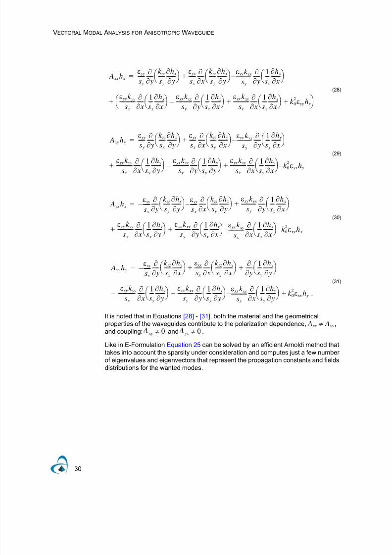
It is noted that in Equations [28] - [31], both the material and the geometricalproperties of the waveguides contribute to the polarization dependence, ,and coupling: and .
Like in E-Formulation Equation 25 can be solved by an efficient Arnoldi method thattakes into account the sparsity under consideration and computes just a few numberof eigenvalues and eigenvectors that represent the propagation constants and fieldsdistributions for the wanted modes.
(28)
(29)
(30)
(31)
A xx h x
ε yy
s y
------ ∂∂ y-----
k zz
s y
-----∂h x
∂ y--------⎝ ⎠
⎛ ⎞ ε yx
s x
------ ∂∂ x-----
k zz
s y
-----∂h x
∂ y--------⎝ ⎠
⎛ ⎞ ε yyk yx
s y
------------ – ∂
∂ y-----
1
s x
----∂h x
∂ x--------⎝ ⎠
⎛ ⎞+=
+ ε yyk yy
s x
------------ ∂∂ x----- 1
s x
----∂h x
∂ x--------⎝ ⎠⎛ ⎞ ε yx k xx
s y
------------ ∂∂ y----- 1
s x
----∂h x
∂ x--------⎝ ⎠⎛ ⎞ – ε yx k xy
s x
------------ ∂∂ x----- 1
s x
----∂h x
∂ x--------⎝ ⎠⎛ ⎞ k 0
2ε yy h x+ +⎝ ⎠⎛ ⎞
A xy h y
ε yy
s y
------ ∂∂ y-----
k zz
s x
-----∂h x
∂ y--------⎝ ⎠
⎛ ⎞ ε yx
s x
------ ∂∂ x-----
k zz
s y
-----∂h y
∂ x--------⎝ ⎠
⎛ ⎞ ε yy k yx
s y
------------ – ∂
∂ y-----
1
s y
----∂h y
∂ x--------⎝ ⎠
⎛ ⎞+=
+ε yy k yy
s x
------------ ∂∂ x-----
1
s y
----∂h y
∂ y--------⎝ ⎠
⎛ ⎞ ε yx k xx
s y
------------ ∂∂ y-----
1
s y
----∂h y
∂ y--------⎝ ⎠
⎛ ⎞ – ε yx k xy
s x
------------ ∂∂ x-----
1
s y
----∂h y
∂ x--------⎝ ⎠
⎛ ⎞ k 02
– ε yx h y+
A yx h x
ε xy
s x
------ – ∂
∂ y-----
k zz
s y
-----∂h x
∂ y--------⎝ ⎠
⎛ ⎞ ε yx
s x
------ – ∂
∂ x-----
k zz
s y
-----∂h x
∂ y--------⎝ ⎠
⎛ ⎞ ε xy k yx
s y
------------ ∂∂ y-----
1
s x
----∂h x
∂ x--------⎝ ⎠
⎛ ⎞+=
+ε xy k yy
s x
------------ ∂∂ x-----
1
s x
----∂h x
∂ y--------⎝ ⎠
⎛ ⎞ ε xx k xx
s y
------------ ∂∂ y-----
1
s x
----∂h x
∂ x--------⎝ ⎠
⎛ ⎞ ε yx k xy
s x
------------ – ∂
∂ x-----
1
s x
----∂h x
∂ x--------⎝ ⎠
⎛ ⎞ k 02
– ε xy h x+
A yy h y
ε xy
s x
------ – ∂
∂ y-----
k zz
s x
-----∂h y
∂ x--------⎝ ⎠
⎛ ⎞ ε xx
s x
------ ∂∂ x-----
k zz
s x
-----∂h y
∂ x--------⎝ ⎠
⎛ ⎞ ∂∂ y-----
1
s y
----∂h y
∂ y--------⎝ ⎠
⎛ ⎞+ +=
ε xyk yy
s x-------------- – ∂∂ x----- 1
s y----∂h y
∂ y--------⎝ ⎠⎛ ⎞ ε xx k xx
s y------------ ∂∂ y----- 1
s y----∂h y
∂ y--------⎝ ⎠⎛ ⎞ ε xx k xy
s x
------------ – ∂∂ x----- 1s y----∂h y
∂ y--------⎝ ⎠⎛ ⎞ k 02ε xx h y .+ +
A xx A yy≠ xy 0≠ yx 0≠

7/21/2019 OptiMode User Reference
http://slidepdf.com/reader/full/optimode-user-reference 35/339
VECTORAL MODAL ANALYSIS FOR ANISOTROPIC W AVEGUIDE
31
Appendix II
H-Formulation
The full vectorial wave equation for is given by:
By substituting into Equation 1 we get:
The term is null.
We can separate Equation 2 into one for longitudinal terms and another one fortransversal terms:
for longitudinal terms, and
By substituting
into the first right hand term of Equation 4, we get:
(1)
(2)
(3)
(4)
(5)
(6)
H
∇ κ˜
∇ H ×× k 02μ0 H – 0=
∇˜
∇˜
t
∂∂ z-----e z+=
∇˜
t k zz ∇˜
t H t×( )× ∇˜
t κ˜
t ∇˜
t H ze z×( )× ∇˜
t κ˜
t
∂∂ z----- e z H t×( )×+ +
+∂∂ z----- e z κ zz ∇
˜t H t×( )×[ ]
∂∂ z----- e z κ
˜t ∇˜
t H ze z×( )×[ ] ∂
∂ z----- e z κ
˜t
∂∂ z----- e z H t×( )⎝ ⎠
⎛ ⎞×+ +
= k 02κ
˜t H t k 0
2k zz H ze z+
∂∂ z----- e z κ zz ∇
˜t H t×( )×[ ]
∇˜
t κt ∇˜
t H ze z×( )× ∇˜
t κt
∂∂ z----- e z H t×( )×+ k 0
2
k zz H ze z=
∇˜
t k zz ∇˜
t H t×( )× ∂
∂ z----- e z κ
˜t ∇˜
t H ze z×( )×[ ] ∂
∂ z----- e z κ
˜t
∂∂ z----- e z H t×( )⎝ ⎠
⎛ ⎞×+ + k 02κ˜
t H t=
H t x y z, ,( ) h t x y z, ,( ) jk 0n0 z – ( )exp=
∇t k zz ∇t H t×( )× ∇t k zz ∇t h t×( )× jk 0n0 z – ( )exp=

7/21/2019 OptiMode User Reference
http://slidepdf.com/reader/full/optimode-user-reference 36/339
VECTORAL MODAL ANALYSIS FOR ANISOTROPIC W AVEGUIDE
32
By substituting Equation 5 into the second right hand term of Equation 4, we get:
The third term of Equation 4 can be rewritten as:
By substituting Equation 5 into the second right hand term of Equation 4, we get:
Where
References
[1] [Berenger, 1994] J. P. Berenger, "A Perfectly Matched Layer for the Absorption ofElectromagnetic Waves," J. Comput. Phys., No. 114, 1994, pp. 185-200.
[2] [Teixeira, 1998] F. L. Teixeira and W. C. Chew, " Systematic Derivation of Anisotropic PML Absorbing Media in Cylindrical and Spherical Coordinates", IEEE Microwave and GuidedLett.,vol. 8, No. 6, pp. 371-373, 1998.
[3] [Huang, 1993] W. P. Huang, C. L. Xu, "Simulation of Three-Dimensional Optical Waveguidesby a Full-Vector Beam Propagation Method”, IEEE J. Quant. Electron., vol. 29, No.10, pp. 2639-2649, 1992.
[4] [Huang, 1992 A] W. P. Huang, C. L. Xu, S. T. Chu and S. K. Chaudhuri, " The Finite-DifferenceVector Beam Propagation Method. Analysis and Assessment”, IEEE J. Light. Techn., vol.10,No.,3, pp. 295-305, 1992.
[5] [Huang, 1996A] W. P. Huang, C. L. Xu, W. Lui, and K. Yokoyama, "The Perfectly Matched LayerBoundary Condition for Modal Analysis of Optical Waveguides: Leaky Mode Calculations",IEEE Photon. Techn. Lett., vol. 8, No. 5, pp. 652-654, May 1996.
(7)
(8)
(9)
(10)
∂∂ z----- e z κ
˜t ∇˜
t H ze z×( )×[ ] e z κ˜
t ∇˜
t
∂h z
∂ z------- jk 0n0h z – ⎝ ⎠
⎛ ⎞ e z×× jk 0n0 z – ( )exp=
∂∂ z----- e z κ
˜t
∂∂ z----- e z H t×( )⎝ ⎠
⎛ ⎞× ∂
∂ z----- p
∂ ht
∂ z-------⎝ ⎠
⎛ ⎞ – =
∂∂ z----- p
∂ ht
∂ z-------⎝ ⎠
⎛ ⎞ – k 02n0
2 ht 2 jk 0n0 p
∂ ht
∂ z------- p
∂ ht
2
∂ z2-------- – +⎝ ⎠
⎛ ⎞ jk 0n0 z – ( )exp=
p k yy k yx –
k xy – k xx
.=

7/21/2019 OptiMode User Reference
http://slidepdf.com/reader/full/optimode-user-reference 37/339
VECTORAL MODAL ANALYSIS FOR ANISOTROPIC W AVEGUIDE
33
[6] [Huang, 1996] W. P. Huang, C. L. Xu, W. Lui, and K. Yokoyama, "The Perfectly Matched Layer(PML) Boundary Condition for the Beam Propagation Method", IEEE Photon. Techn. Lett., vol.8, No. 5, pp. 649-651, May 1996.
[7] [Huang, 1992 B] W. P. Huang and C. L. Xu, "A Wide-Angle Vector Beam Propagation Method”,
IEEE Photon. Techn. Lett., vol. 4, No. 10, pp. 1118-1120, 1992.[8] [Hadley, 1992] G. R. Hadley, "Wide-Angle Beam Propagation using Padé Approximant
Operators", Opt. Lett., vol. 17, No. 20, pp. 1426-1428, 1992.
[9] [Van, 1992] H. A. Van Der Vorst, "Bi-CGSTAB: A Fast and Smooth Converging Variant of Bi-CGfor the Solution of Nonsymmetric Linear System”, SIAM J. Sci. Statist. Comput., vol. 13, pp.631-644, 1992.
[10] [Mielewski, 1998] J. Mielewski and M. Mrozowski, “Application of the Arnoldi Method in FEM Analysis of Waveguides", IEEE Microwave and Guided Lett. vol. 8, No.1, pp. 7-9, 1998.
[11] [Huang, 1991] W. P. Huang, C. L. Xu, and S. K. Chaudhuri, " A Finite-Difference Vector BeamPropagation Method based on H-Fields”, IEEE Photon. Tech. Lett., vol. 3, pp. 1117-1120, 1991.
[12] [Huang, 1994] Xu, C. L., W. P. Huang, J. Chrostowski, and S. K. Chaudhuri, "A Full-VectorialBeam Propagation Methods for Anisotropic Waveguides”, IEEE J. Lightwave Tech., vol.12, No.11, pp. 1926-1931.

7/21/2019 OptiMode User Reference
http://slidepdf.com/reader/full/optimode-user-reference 38/339
VECTORAL MODAL ANALYSIS FOR ANISOTROPIC W AVEGUIDE
34

7/21/2019 OptiMode User Reference
http://slidepdf.com/reader/full/optimode-user-reference 39/339
35
Fiber Mode Solvers
Introduction
Many kinds of optical fiber can be described, or in the case of graded index fibers,approximated by, a series of concentric layers of loss-less dielectric. When the indexcontrast in the structure is small, it is common to use the scalar wave equation to
obtain the linearly-polarized modes (LP modes). However, when the index contrastbecomes larger, the LP approximation becomes inaccurate, and a full vector analysisis necessary [1]. Within any one of the concentric layers, the field components are alllinear combinations of Ordinary and Modified Bessel functions, and the solution is amatter of matching the tangential field components of adjacent layers, leading to thesolution of a linear system. There are some choices to make about the best way toarrange the linear system (see Ref. [2] for a complete treatment) but probably the bestchoice for a general, quick algorithm is the method of Yeh and Lindgren [3]. Themethod has intuitive appeal in its similarity to the transfer matrix method used for theanalysis of planar waveguides [4]. Both methods use a matrix to express the fields atone side of a layer given their values at the other side, and the whole structure is thencharacterized by cascading the layers by matrix multiplication. For vector fields infibers, there is no natural separation into TE and TM polarization, so one must includethe two tangential components for both electric and magnetic field simultaneously. Intotal there are four transverse components at the layer boundaries, so the transfermatrix in fiber is a 4x4 matrix, instead of 2x2.
The method used by the Optiwave fiber mode solvers is different from the previousworks in three ways. The 4x4 matrix method for vector modes in fibers isimplemented with these improvements to make the algorithm faster in execution time,and more reliable in the finding of modes, particularly in cases where the modes arealmost degenerate. The first improvement involves a reformulation of the basicequations to make a real-valued numerical implementation. Since it is loss-lessmodes on a fiber of loss-less material that is being sought, there is no reason toinclude complex numbers in the formulation. Real-valued implementation uses lesscomputer resources. Second, the complete transfer across one layer boundaryrequires a matrix inverse. It is better to find this inverse analytically, rather than relyon numerical inversion at each stage. The layer matrix can be decomposed into two4x4 matrices, and the new matrices are of a form where it is easy to find the inverseby inspection, thereby finding the analytic solution to the original inversion problem.Third, it is usual to construct the dispersion function (the zeros of which are located atthe modal indices) as the determinant of the 4x4 matrix system. While this istheoretically correct, it is not the most intuitive prescription. Worse, the determinant

7/21/2019 OptiMode User Reference
http://slidepdf.com/reader/full/optimode-user-reference 40/339
is not the most convenient construction for locating the zeros, particularly in the casewhere two zeros are very close to each other. Optiwave uses an eigen-value analysisthat splits the dispersion function into two functions. This splitting resolves the almostdegenerate pairs and helps the simple-minded computer algorithms to find the zerosof the dispersion function (i.e. the modes) more reliably.
Real-valued formulation
The time independent Maxwell curl equations with a positive time convention ( )are
and the divergence equations are
The factor j does not suit the current purpose, so make the substitution
where is the free space impedance, so that h and E have the sameunits. Then
where . Eliminating the h gives the electric wave equation
Debye Potential
For finding electromagnetic fields in a cylindrical geometry it is convenient to usecylindrical coordinates r, and z, and Debye potentials parallel to the axis of rotation,
[2]
(1)
(2)
(3)
(4)
(5)
(6)
(7)
e jωt
E∇× jωμ 0H – = H∇× jωε 0εE=
∇ εE( )⋅ 0= ∇ H⋅ 0=
h jη0H – =
η0 μ 0 ε ⁄ 0=
E∇× k h= h∇× k εE=
k ω μ 0ε 0=
∇ ∇ E k 2
– ×× εE 0=
θ
z
E ∇ zψ( )× 1
k ε-----∇ ∇ zϕ( )××
+=
h ∇ zϕ( )× 1
k ---∇ ∇ zψ( )××+=
7/21/2019 OptiMode User Reference
http://slidepdf.com/reader/full/optimode-user-reference 41/339
FIBER MODE SOLVERS
37
It is supposed that the permittivity is constant in the region in which the aboveequations apply. The fibers are defined as a series of concentric layers of constantdielectric, so for the fiber mode solver, the region is the annulus between the layerboundaries. Equation 6 and Equation 7 are applied in a piecemeal way. Strictlyspeaking, the , and should have subscripts to indicate to which layer thesolution applies, but they are dropped here to simplify the representation. The
complete solution for the multilayer fiber will be constructed by using a separate pairof functions for each layer, and by matching the tangential field components at thelayer boundaries
The divergence of the curl of any vector field is identically zero. Therefore the choiceof (6) and (7) to represent the electric and magnetic fields means that the divergenceequations (2) will automatically be satisfied. In the remainder of this section, we showthat if the two potentials and are solutions to the scalar Helmholtz equation, then(6) will be a solution to the Maxwell wave equation (5), at least within any given layer.In subsequent sections, the particular solution for the mode will be found by observingthe boundary conditions imposed by physical considerations on E and h.
Suppose is a continuous function of position that satisfies the Helmholtz equation
in 3 dimensions
Consider the following equation, true for any satisfying (9) in a region of constantpermittivity.
Associate the first two terms together and apply the vector identity
to get
The right hand side of (11) is a gradient of a scalar function, so the curl of the left handside must be zero. take the curl of (11)
(8)
(9)
(10)
(11)
(12)
ψ ϕ ε
ψ ϕ
ψ
∇2ψ k 2εψ+ 0=
ψ
∇ ∇ zψ( )⋅[ ] ∇2zψ( ) – k
2εzψ – ∇∂ψ∂ z-------=
∇ ∇ ⋅( ) ∇2 ∇ ∇ ××= –
∇ ∇ zψ( )×× k 2εzψ – ∇∂ψ
∂ z-------=
∇ ∇ ∇ zψ( ) k 2ε∇ zψ( )× – ××× 0=

7/21/2019 OptiMode User Reference
http://slidepdf.com/reader/full/optimode-user-reference 42/339
FIBER MODE SOLVERS
38
and define E by the first term of (6). With E defined this way, the Maxwell electricwave equation (5) follows, and therefore this E is a possible solution for electric field.
Solutions defined from the function solely (that is to say, solutions with = 0), willhave electric fields of the form
from which we can see there is no longitudinal (z) component to the electric field, i.e.these are transverse electric fields. The magnetic field associated with thesetransverse electric fields is constructed from the first Maxwell curl equation in (4):
which is the second term of (7).
The same sequence (7) - (11) can be applied to the function to give transversemagnetic fields, and the electric components of these are given as the second termof (6). A linear superposition of transverse magnetic and transverse electric fields willgive solutions that are neither transverse magnetic nor transverse electric. In fact,most modes of the fiber are of this hybrid kind. In the hybrid case, equations (6) and(7) are used as written, and the relative value of the and is now important, sinceit is a specific linear combination that matches the boundary conditions at the layerboundaries.
Separation of Variables
The potentials themselves are solutions of the scalar Helmholtz equation, and theparticular solution is found by observing the boundary conditions imposed by physicalconsiderations on E and h. The potentials are supposed to form modes, so a solutionwhere the variables are separated is appropriate
and a similar expression applies for the other Debye potential, . The Helmholtzequation (8) is expanded in cylindrical co-ordinates, and then (15) is substituted.Forregions where is constant, the radial functions follow the Ordinary or ModifiedBessel equation, and so the solutions are linear combinations of Bessel functions ofinteger order v. In any given layer,
(13)
(14)
(15)
(16)
ψ ϕ
E ∇ ψz( ) r
r --=× ∂ψ
∂θ------- θ∂ψ
∂r ------- – =
h 1
k ---∇ ∇ zψ( )××=
ϕ
ψ ϕ
ψ r θ z, ,( ) ψν r ( ) j νθ β z – ( )[ ]exp=
ϕ
ε
ϕν r ( ) AJ ν ur ( ) BY ν ur ( )+= ψν r ( ) CJ ν ur ( ) DY ν ur ( )+=
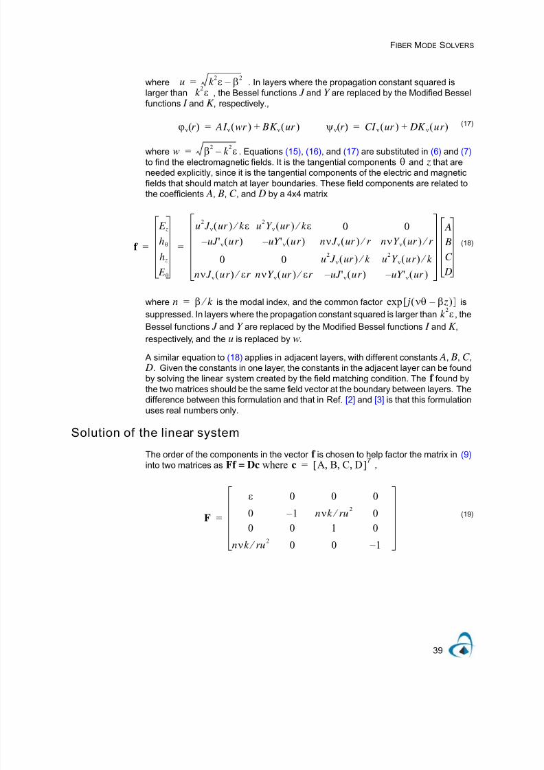
7/21/2019 OptiMode User Reference
http://slidepdf.com/reader/full/optimode-user-reference 43/339
FIBER MODE SOLVERS
39
where . In layers where the propagation constant squared islarger than , the Bessel functions J and Y are replaced by the Modified Besselfunctions I and K , respectively.,
where . Equations (15), (16), and (17) are substituted in (6) and (7) to find the electromagnetic fields. It is the tangential components and z that areneeded explicitly, since it is the tangential components of the electric and magneticfields that should match at layer boundaries. These field components are related tothe coefficients A, B, C , and D by a 4x4 matrix
where is the modal index, and the common factor is
suppressed. In layers where the propagation constant squared is larger than , the
Bessel functions J and Y are replaced by the Modified Bessel functions I and K ,
respectively, and the u is replaced by w.
A similar equation to (18) applies in adjacent layers, with different constants A, B, C , D. Given the constants in one layer, the constants in the adjacent layer can be foundby solving the linear system created by the field matching condition. The f found bythe two matrices should be the same field vector at the boundary between layers. The
difference between this formulation and that in Ref. [2] and [3] is that this formulationuses real numbers only.
Solution of the linear system
The order of the components in the vector f is chosen to help factor the matrix in (9) into two matrices as Ff = Dc where ,
(17)
(18)
(19)
u k 2ε β2
– =k
2ε
ϕν r ( ) AI ν wr ( ) BK ν ur ( )+= ψν r ( ) CI ν ur ( ) DK ν ur ( )+=
w β2k
2ε – =θ
f
E z
hθ
h z
E θ
u2 J ν ur ( ) k ε ⁄ u
2Y ν ur ( ) k ε ⁄ 0 0
uJ 'ν ur ( ) – uY 'ν ur ( ) – nν J ν ur ( ) r ⁄ nνY ν ur ( ) r ⁄
0 0 u2 J ν ur ( ) k ⁄ u
2Y ν ur ( ) k ⁄
nν J ν ur ( ) εr ⁄ nνY ν ur ( ) εr ⁄ uJ 'ν ur ( ) – uY 'ν ur ( ) –
A
B
C
D
= =
n β k ⁄ = j νθ β z – ( )[ ]expk
2ε
c A B C D, , ,[ ]T =
F
ε 0 0 0
0 1 – nνk ru2 ⁄ 0
0 0 1 0
nνk ru 2 ⁄ 0 0 1 –
=

7/21/2019 OptiMode User Reference
http://slidepdf.com/reader/full/optimode-user-reference 44/339
FIBER MODE SOLVERS
40
The advantage of this factoring is that it is easy to find the expressions for and. is found by two row reductions and by inverting the 2x2 matrices in the
block diagonal. These matrices are required to find the coefficients in the next layer.If are the coefficients in the m-th layer, then the coefficients in the next layer isfound from the matrix product,
The use of the factored matrix means four matrix multiplications instead of two arerequired to cross the boundary, but it avoids having to find the matrix inversenumerically.
Dispersion equation
The matrix to describe the whole multilayer can be written as one 4x4 matrix, theproduct of all layers, one layer of which is shown in (21). The dispersion equation isusually constructed by setting the determinant of this 4x4 matrix product to 0, but thisis not a good choice from the numerical point of view. In the limit of low index contrast,the modal indices can be very close to each other, making them hard to find bynumerical methods, which tend to skip over closely spaced zeros. A more convenient
condition comes from using rectangular matrices at the first and last layers, which arespecial cases. In the first layer, which contains r = 0, coefficients and mustbe zero, so the first matrix, , is 4 x 2 consisting of the first and third columns of theD matrix in (20). Similarly, in the last layer, it is the coefficients and that mustgo to zero in (17), since those contain solutions with unphysical growth. The lastmatrix will be of size 2 x 4, and consist of the first and third rows of . Theproduct of all these matrices will be of size 2x2, which we call S(n). (The dependenceon n is written explicitly since it is the modal index to be found). A mode is obtainedat a modal index n when a non-trivial solution is found to ,
The condition det(S) = 0 is sufficient for a non-trivial solution. However this conditioncan be inconvenient for the case of certain modes of the low index contrast fiber. Forexample, consider a step index fiber with radius 2 , having a core index of 1.46and a cladding of 1.45. For order zero ( ), the determinant of S will vary withthe modal index n as shown in Figure 1.
(20)
(21)
(22)
D
u2 J ν k ⁄ u
2Y ν k ⁄ 0 0
uJ 'ν uY 'ν 0 0
0 0 u2 J ν k ⁄ u2Y ν k ⁄ 0 0 uJ 'ν uY 'ν
=
F 1 –
D 1 –
F 1 –
D 1 –
cm
cm 1+ Dm 1+
1 – r m( )Fm 1+ r m( )Fm
1 – r m( )Dm r m( )cm=
B0 D0
D0
A M C M
Iν
D M
1 – D
1 –
0 S n( ) A0
C0
=
μmν 0=
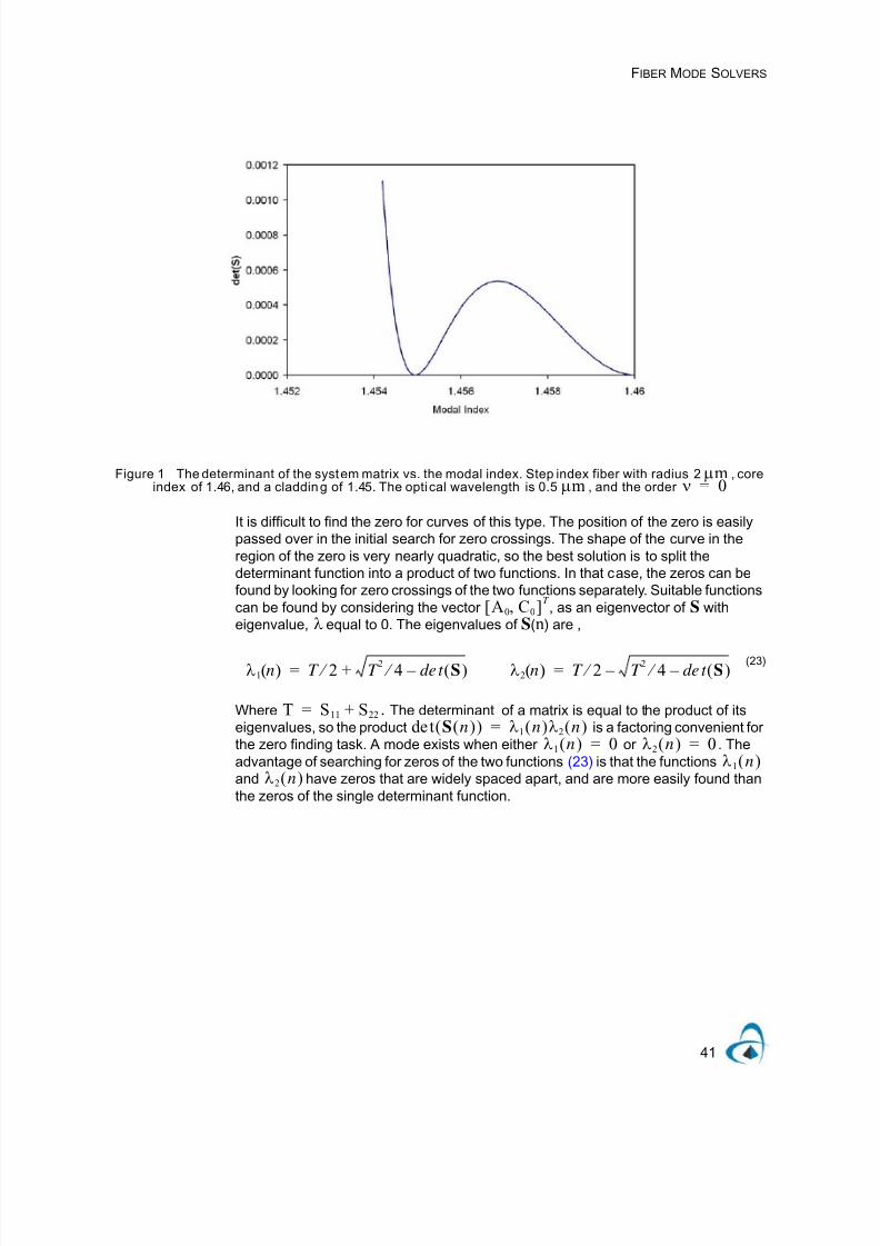
7/21/2019 OptiMode User Reference
http://slidepdf.com/reader/full/optimode-user-reference 45/339
FIBER MODE SOLVERS
41
Figure 1 The determinant of the system matrix vs. the modal index. Step index fiber with radius 2 , coreindex of 1.46, and a cladding of 1.45. The optical wavelength is 0.5 , and the order
It is difficult to find the zero for curves of this type. The position of the zero is easilypassed over in the initial search for zero crossings. The shape of the curve in theregion of the zero is very nearly quadratic, so the best solution is to split thedeterminant function into a product of two functions. In that case, the zeros can befound by looking for zero crossings of the two functions separately. Suitable functionscan be found by considering the vector , as an eigenvector of S witheigenvalue, equal to 0. The eigenvalues of S(n) are ,
Where . The determinant of a matrix is equal to the product of itseigenvalues, so the product is a factoring convenient forthe zero finding task. A mode exists when either or . Theadvantage of searching for zeros of the two functions (23) is that the functionsand have zeros that are widely spaced apart, and are more easily found thanthe zeros of the single determinant function.
(23)
μmμm ν 0=
A0 C0,[ ]T
λ
λ1 n( ) T 2 ⁄ T 2
4 ⁄ de t S( ) – += λ2 n( ) T 2 ⁄ T 2
4 ⁄ de t S( ) – – =
T S11 S22+=det S n( )( ) λ1 n( )λ2 n( )=
λ1 n( ) 0= λ2 n( ) 0=λ1 n( )
λ2 n( )

7/21/2019 OptiMode User Reference
http://slidepdf.com/reader/full/optimode-user-reference 46/339
FIBER MODE SOLVERS
42
Figure 2 Plot of the eigenvalues and determinant vs modal index.
Figure 3 Expanded view of the zero crossing region
LP Modes
Linearly Polarized modes can be found with the same style of approach as above, bya transfer matrix analysis of multilayer fibers.In the LP analysis, the initial excitation isassumed to have a linear polarization, and so a modal analysis supporting only one

7/21/2019 OptiMode User Reference
http://slidepdf.com/reader/full/optimode-user-reference 47/339
FIBER MODE SOLVERS
43
field component is used. It can be shown this is a good approximation for fibers withlow refractive index contrast, as shown below.
Consider again the wave equation of (5), but this time use the vector identity (10) directly on the electric wave equation instead of introducing the Debye potential. The
result is
From the Maxwell divergence equation (2)
so that
In the case of low index contrast waveguides, such as are found in most optical fibers,the last term in (26) is negligible. The last term is the only one that contributes tocoupling among the field components of the electric field, so if this term is neglected,the model will be a polarization preserving model. If the excitation was a linearpolarization parallel to the X axis, the model could be further simplified by consideringonly the X component of (26). This shows that for the LP model, the governingequation for the field is the Helmholtz equation (8) applied to the field component .
The solution for LP modes is constructed in a similar way as for the vector modes.The is constructed in each layer as a linear combnation of Bessel functions (16) and (17), except this time only two coefficients, and , are required, since only
one function needs to be constructed. The physical consideration at the layerboundaries is the continuity of and its derivative. The two conditions are related tothe two coefficients A and B for each layer by 2x2 matrices. The modes are found bysetting up a calculation that assumes and for the first (inner most)layer, and then calculating the coefficients in each subsequent layer by matrixmanipulations. The last layer has the condition that the coefficient ( ) of the Besselfunction must be zero, since this Bessel function is not bounded at infinity. Thislast coefficient is a function of the order and the modal index n, so the modes arefound by finding the zeros of .
(24)
(25)
(26)
∇2E ∇ ∇ E⋅( )E – k
2+ εE 0=
0 ∇ εE( )⋅ E ∇ε ε ∇ E⋅( )+⋅= =
∇2E k
2εE ∇ E ∇ε
ε
-------⋅⎝ ⎠
⎛ ⎞+ + 0=
E x
E x
A1 B1
E x
A1 1= B1 0=
A M
Iνν
A M n( )

7/21/2019 OptiMode User Reference
http://slidepdf.com/reader/full/optimode-user-reference 48/339
FIBER MODE SOLVERS
44
References
[1] K. Okamoto, Fundamentals of Optical Waveguides, (Academic Press, San Diego, 2000).
[2] C. Tsao, Optical Fibre Waveguide Analysis, (Oxford University Press, 1992), Part III
[3] C. Yeh and G. Lindgren, "Computing the propagation characteristics of radially stratified fibers:an efficient method", Applied Optics 16(2) p483-493 (1977)
[4] J. Chilwell and I. Hodgkinson, "Thin-films field-transfer matrix theory of planar multilayerwaveguides and reflection from prism-loaded waveguide", Journal of the Optical Society of
America A, 1 p742-753 (1984)
7/21/2019 OptiMode User Reference
http://slidepdf.com/reader/full/optimode-user-reference 49/339
45
Finite Difference Mode Solver
Introduction
This mode solver uses a magnetic field based formulation of the difference equationsto convert the mode solving problem into a problem of finding eigenvectors of a largesystem of linear equations. The formulation is due to Lüsse [1]. Once the linear
system is found from this formulation, the modes can be found by findingeigenvectors, and for this we use the Implicitly Restarted Arnoldi Method (IRAM), asimplemented by ARPACK [2]. In OptiMode, the boundary condition applied at theedges of the calculation window can be of the Dirichlet type (magnetic field goes tozero at the window boundaries), or the user can select “Transparent BoundaryConditions” (TBC). In the TBC case, the algorithm will try to match the optical field atthe boundary to a plane wave with propagation constant constructed from theapproximate modal field available at intermediate stages of the simulation. Thispropagation constant is complex, so it should be able to accommodate leakingradiation as well as the more common exponential decay of the field.
The operation of the IRAM and the TBC are controlled from settings parameters inOptiMode. These parameters are found in the FD tab of the Solver Parameters dialog
box (Fig. 2). The parameters that control the eigenvector solving are Tolerance, Max.Steps, Preview Mode, Skip Value, and Dimension of the Krylov Subspace. Thistechnical background is intended to explain what these parameters mean and howthey influence the mode solving. The values of the parameters are pre-set to valuesthat seem to work well for most cases. However, there could be exceptional cases inwhich the user will need to modify those parameters. This technical background isprovided to help the user understand what these parameters do and what mighthappen if they are changed.
We provide a summary of the Lüsse formulation of the finite difference equations foroptical magnetic field. Then we show an overview of how the IRAM works, not in greatdetail, but simply enough to show the meaning of the OptiMode Settings parameters.Then we show how the TBC is constructed, so that its behaviour can be understood.

7/21/2019 OptiMode User Reference
http://slidepdf.com/reader/full/optimode-user-reference 50/339
Magnetic Formulation
Inside a dielectric, the time independent Maxwell curl equations with a positive timeconvention ( ) are
and the divergence equations are
In the magnetic formulation, the electric field is eliminated from (1) by taking the curlof the second equation and substituting from the first. For regions of constantpermittivity , there are no gradients of , and the equation simplifies to
In view of the vector identity , and the property ofhaving zero divergence, (3) becomes
where is the free space wavenumber.
It is true that it is usually the electric field, and not the magnetic field, that is of interestfor applications. The motivation for solving the problem with a magnetic formulation isthat the waveguide structure is created by introducing discontinuities in electricpermittivity, , and not magnetic permeability, . When matching boundary
conditions at layer boundaries, the normal component of the electric field isdiscontinuous, since it is the electric displacement, , and not the electricfield that is to be made continuous. Since the permeability is the vacuum leveleverywhere, all components of the magnetic field are continuous at all boundaries.The finite difference representation of continuous functions is more accurate thandiscontinuous functions, and therefore a finite difference formulation based on themagnetic field gives more accurate results than one based on electric fields.
The electric fields are still needed for applications. These fields can be calculated afterthe fact by taking the curl of the magnetic field (using the second equation in (1)) byfinite differences. Explicitly,
(1)
(2)
(3)
(4)
(5)
(6)
e jω t
E∇× jωμ 0H – = H∇× jωε 0εE=
∇ εE( )⋅ 0= ∇ H⋅ 0=
ε ε
H∇×∇× ω2μ0ε0εH=
A∇×∇× ∇ ∇ A⋅( ) ∇2A – =
H
∇2H k
2εH+ 0=
k ω μ0ε0=
ε μ
D εε 0E=μ0
E x η – 0
k ε-------- 1
β---
y x∂
2
∂∂ H x 1
β---
y2
2
∂∂ H y β H y – +
⎝ ⎠⎜ ⎟⎛ ⎞=
E y
η0
k ε-----
1
β---
x2
2
∂
∂ H x 1
β---
x y∂
2
∂∂ H y β H x – +
⎝ ⎠⎜ ⎟⎛ ⎞
=

7/21/2019 OptiMode User Reference
http://slidepdf.com/reader/full/optimode-user-reference 51/339
FINITE DIFFERENCE MODE SOLVER
47
In the mode solving problem, the permittivity does not vary with z, and so thesolution for the magnetic field can be expected to be an harmonic function of z:
and (7) in (4) gives
Since the is unknown, the mode solving problem is really an eigenvector problemwith as the eigenvalue, and the function or as theeigenfunction.
Magnetic Finite Difference Equations
In order to reduce the partial differential equation into difference equations for solving,a mesh needs to be defined and applied. The mesh used is shown in Fig. 1 below. Itshows a sample of the mesh at a point P that is not on one of the calculation windowboundaries. The magnetic fields are defined at the nodes (dots at the intersections),and the permittivity is defined in the rectangular regions bounded by the nodes. Thepermittivity inside the rectangular regions , , , and is taken to beconstant, so inside each of these regions, the equations (8) and (9) apply.
Figure 1 Mesh for the finite diff erence equation. The magnetic field is defined at points N, S, E, W, and P.The permittivity is defined in the rectangular regions bounded by the nodes.
(7)
(8)
(9)
ε
H x y z, ,( ) h x y,( )e
jβ z –
=
∂2h x
x2∂
---------- ∂2
h x
y2∂
---------- k 2εh x+ + β2
h x=
∂2h y
x2∂
---------- ∂2
h y
y2∂
---------- k 2εh y+ + β2
h y=
ββ2 h x x y,( ) h y x y,( )
ε NE ε NW εSE εSW

7/21/2019 OptiMode User Reference
http://slidepdf.com/reader/full/optimode-user-reference 52/339
FINITE DIFFERENCE MODE SOLVER
48
The mesh is in the transverse plane, and (8) and (9) do not, by themselves, introducecoupling between the field components and . The couplingcomes from matching the transverse components of electric and magnetic fields atthe boundaries.
In Ref [1], the magnetic fields inside the rectangular regions are expanded to the
second order in derivatives defined at the centre point, P. Those expansions are usedto estimate what the longitudinal components and will be at the horizontaland vertical boundaries between the points N, S, E, W, and P. Once this is done, anequation involving the magnetic field components at the nodes is eventually obtained:
Equation (10) comes mostly from (8) for . In the matching of transversecomponents of the fields, another term involving appears. This is the term that isresponsible for the coupling of and . In the finished finite differenceformulation, the derivative of with respect to x is replaced by a centred finitedifference. Note that if at this particular node, it happens that the permittivity is thesame on the north side of the boundary as on the south (i.e. it is a vertical boundary),no coupling will occur, or at least there will be no contribution from the componentof this node.
This equation (and a similar one for ) is applied to each node in the mesh. Let thenumber of nodes be n. It is the repeated application of this equation, and theadjustment of the meaning of the N, S, W, E, and P designations, that generates alarge system of linear equations. The values of the x and y components of themagnetic field are collected in a vector of dimension n x 1, called , say. Theequations on the left form an n x n matrix that multiplies , and the right handside has the original vector representing the magnetic field, multiplied by theeigenvalue . In vector-matrix form, the problem looks like
and to find the modal indices ( ) and modes, , is a matter of solvinga classical eigenvector problem.
Implici tly Restarted Arnoldi Method (IRAM)
The repeated application of (10) for every node, and the application of a similarequation for leads to an eigenvector problem of a large system of linear
(10)
(11)
h x x y,( ) h y x y,( )
e z h z
h xE
Δ x2
-------- h xW
Δ x2
-------- h xN
Δ y2
-------- εSE
ε NE εSE +---------------------
εSW
ε NW εSW +----------------------+
h xS
Δ y2
-------- ε NE
ε NE εSE +---------------------
ε NW
ε NW εSW +----------------------+
h xP
k 2ε NW εSW
ε NW εSW +----------------------
k 2ε NE εSE
ε NE εSE +---------------------
2
Δ y
2--------
2
Δ x
2-------- – – +
h y∂ x∂
------- 1
Δ y------
ε NW εSW –
ε NW εSW +----------------------
ε NE εSE –
ε NE εSE +---------------------+
+ +
+
+
+ β2h xP=
h x
h y
h x h y
h y
h y
h y
vQ v
β2
Qv β2v=
nmo d β k ⁄ = v
h y
7/21/2019 OptiMode User Reference
http://slidepdf.com/reader/full/optimode-user-reference 53/339
FINITE DIFFERENCE MODE SOLVER
49
equations. The Finite Difference Mode Solver uses the Implicitly Restarted ArnoldiMethod as described in Ref. [2] to find the eigenvectors of this system, and therebyfind the modes of the waveguide.
The Implicitly Restarted Arnoldi Method looks for the modes inside a Krylov
Subspace. This subspace is constructed from the mode operator, and from anarbitrary (could be random) starting magnetic field, here described as a vector, .The Krylov subspace is the space spanned by powers of the when applied to the initial vector :
The IRAM constructs a basis for the dimensional Krylov subspace by theGram-Schmidt process. For example, a basis for a 2 dimensional Krylov subspace,
, can be constructed from and . A vector perpendicular tocan be found by subtracting the component from :
This vector is parallel to the second basis vector, , which is found once isdivided by its length, . It is easy to show that this length is
The above inner product of with occurs frequently, so the matrix componentsare defined
With this definition, the effect of including another power of can be written in termsof the new basis vectors
Following the Gram-Schmidt process, a vector in the Krylov subspace that isperpendicular to both and can be constructed from subtracting theprojections of onto the first two basis vectors
Normalizing as before, and rearranging terms shows how the space generatedfrom can be represented in terms of the basis vectors
(12)
(13)
(14)
(15)
(16)
(17)
(18)
v1
K m Q v1 ),( Qv1
K m Q v1,( ) span v1 Qv1 Q2v1 Q
3v1 …Q
mv1, , , ,{ }=
m 1+
K 1 Q v1 ),( v1 Qv1 v1
v1 Qv1
w2 Qv1 v1T Qv1( )v1 – =
v2 w2
w2
T w2
w2
T w2 v2
T Qv1=
v Q
hij vi
T Qv j=
Q
Qv1 h11v1 h21v2+=
v1 v2
Qv2
w3 Qv2 h – 12v1 h22v2 – =
w3
Q2v1
Qv2 h12v1 h+ 22v2 h32v3+=

7/21/2019 OptiMode User Reference
http://slidepdf.com/reader/full/optimode-user-reference 54/339
FINITE DIFFERENCE MODE SOLVER
50
The Gram-Schmidt process can be followed in as many steps as necessary to createa basis for the Krylov subspace.
An important point to note is that the dimension of , (and therefore thenumber of basis vectors needed to span it), might be less than m + 1. Let’s suppose
that the mode solving problem was asked to find the first k modes, where k < m. Letus also suppose that the initial vector happened to be a linear combination ofthese k modes. Modes are solutions to the eigenproblem of equation (11). Let the ithmode field be represented by , and let its propagation constant (eigenvalue) be
. Call the subspace spanned by those k modes , to represent a subspace ofk dimensions. Then
When the second vector to span the Krylov subspace is calculated, it is apparent it is
also a linear combination of the k eigenvectors, and is therefore still in the subspace,. It is easy to see that this situation is not changed by multiplying by again,
and so
for any power of . ( can be 1, 2, ... up to ). Therefore the dimension of thisKrylov subspace, is fewer than the m + 1 vectors in the span (12). Forthis choice of , the Krylov subspace has dimension k ( < m), and some of thevectors in (12) have linear dependence on others.
When is a member of the subspace , the Gram-Schimdt process mustterminate at k, since having m basis vectors is not possible in . The terminationwill be seen at the kth step of the process, in trying to calculate a vector perpendicularto the previous k basis vectors. Equation (17) showed the generation of the 3rd vector,the kth will be formed from
When this is done with , the must be zero, and the Gram-Schmidtprocess will terminate. Because of the termination, the search for modes will takeplace in a space of dimension k ( 1, 2, maybe 10) rather than in the space of thevectors themselves. The vectors have dimension equal to the number of nodes in the
mesh of Fig. 1. This is typically some number on the order of 105
or 106
. Thistermination greatly simplifies the problem!
Of course, a random choice of is unlikely to be a member of , but the IRAMstrategy is to use iterative processes that effectively change the initial choice ofto a vector inside (or not far from) the subspace .
(19)
(20)
(21)
(22)
K m Q v1 ),(
v1
ei
βi
2S k
v1 x1e1 x2e2 … xk ek + + += S k ∈
Qv1 β1
2 x1e1 β2
2 x2e2 … βk
2 xk ek + + += S k ∈
S k Q
Q jv1 S k ∈
Q j ∞K m Q v1 ),(
v1
v1 S k S k
wk 1+ Qvk h – 1k v1 h2k v2 … hkk vk – – – =
v1 S k ∈ wk 1+
v1 S k
v1
S k

7/21/2019 OptiMode User Reference
http://slidepdf.com/reader/full/optimode-user-reference 55/339
FINITE DIFFERENCE MODE SOLVER
51
In the FD tab of the Solver Parameters dialog box of OptiMode, both k and m aredefined as shown in Fig. 2.
Figure 2 Solver Parameter dialog box of OptiMode disp laying the tab for the Finite Difference mode solver(FD). Dimension of Krylov Subspace (m) and number of modes to find (k) are defined here.
In this example, the IRAM will construct a basis for a Krylov subspace of dimensionm. The default for the dimension of the Krylov subspace is 100. This number was theresult of many mode solving trials. For typical mode solving problems, this numberwas found to be close to optimum. This will involve making m copies of the field
initially found on the defined mesh. m = 100 will occupy a lot of RAM, but it seems tomake the mode solver find the mode more quickly. If this mesh is already very large,there is a possibility to create an out-of-memory error, because the mode solverrequires at least m times the storage required for a single mode. If the memory isexhausted for your problem, try again with a smaller number for m (the dimension ofthe Krylov subspace). m can be made as small as twice the number of modes sought(k) and still get correct results, even if it takes longer to find them.
The first choice of will probably not be anywhere near , so the IRAM beginsa process of shifted Q-R iteration to move away from unwanted eigenvalues andcloser to the desired ones. When the Q-R iteration process is finished, The algorithmrestarts (the R in IRAM). It reduces the dimension of the working space to k, but thenew subspace is different because the QR iterations indirectly change the starting
vector, . The result is usually movement toward the desired solution space .This leaves a new set of vectors spanning a new k dimensional space, and thealgorithm starts the Arnoldi process again to build the dimension up to m. Thenanother Q-R process will start to move closer to . See Ref [2] for details. If youwatch the computer’s Task Manager while the algorithm runs, you might see the usedRAM cycle as the dimension of the space cycles from k to m and back. After many
v1 S k
v1 S k
S k

7/21/2019 OptiMode User Reference
http://slidepdf.com/reader/full/optimode-user-reference 56/339
FINITE DIFFERENCE MODE SOLVER
52
iterations the stopping condition will be met, and at this point the generalization ofequation (18) will appear as
If the is now inside , the last coefficient in the sum will be zero. This is evidentfrom the definition of . If really is inside , is also inside and itmust be perpendicular to , making . In the practicalimplementation of the mode solving problem, won’t be exactly zero, but theIRAM process finishes when it is small enough to be negligible. Once the problem isin the form of (23) with the last term very small, it is easy to find the modes andpropagation constants.
To see this, make the following change in notation. Define an n x k matrix , thecolumns of which are made from the k Arnoldi basis vectors of size n x 1,
and form a k x k matrix from the coefficients of equation (15). Now consider .Equations (16) and (18) show how the first two columns of are formed in termsof and the found in the first three columns of . The reader can find thefollowing columns by following the Gram-Schmidt process further. Note that hasall zero elements for those below the first subdiagonal, because the ith column of
is a linear combination of the first i + 1 basis vectors . (A matrix of this formis called “Hessian”).
All of the columns of , except for the last one, are calculated by . The lastcolumn (kth column), according to (23) will need to include a term . This isn’tavailable in , so the relation is made complete by adding the last column explicitly:
is the kth unit column vector in a k dimensional space, and the transpose is. Putting this row vector after the column vector serves
to put in the last column of a k x k matrix with zeros elsewhere. The secondterm on the right adds the missing column in the relation. From the above discussion,
(23)
(24)
(25)
(26)
Qvk h1k v1 h+ 22v2 … hkk vk hk 1 k ,+ vk 1++ + +=
v1 S k
hij v1 S k Qvk S k
vk 1+ hk 1 k ,+ 0=hk 1 k ,+
V k
vk
V k v1 v2 v3 … vk , , , ,[ ]=
hij QV k
QV k
hij vk V k
H k
QV k vk
H k
h11 h12 h13
h21
h22
h23
0 h32 h33
… h1 k 1 – , h1k
… h2 k 1 – ,
h2k
… h3 k 1 – , h3k
0 0 h43
… … …
0 0 …
… h4 k 1 – , h4k
… … …
0 hk k 1 – , hkk
=
QV k V k H k
vk 1+
V k
QV k V k H k hk 1 k ,+ vk 1+ ek
T +=
ek
ek
T 0 0 0 … 1, , , ,( )= vk 1+
vk 1+

7/21/2019 OptiMode User Reference
http://slidepdf.com/reader/full/optimode-user-reference 57/339
FINITE DIFFERENCE MODE SOLVER
53
the is expected to be small, and it becomes a measure of the accuracy of thesolution.
The k modes we are looking for are inside . These modes can be found by findingthe eigenvectors of the matrix . This greatly simplifies the problem. The matrix
is n x n, where n is the number of nodes in the finite difference mesh. n is typicallyon the order of 105 or 106. On the other hand is k x k, and k is probably of orderof 10 or so. The reduction to (26) simplifies the problem by many orders of magnitude.
The k modes inside are a linear combination of the basis for that space. Let avector, of size k x 1, , represent an arbitrary vector in this space
Now let be an eigenvector of , and let the corresponding eigenvalue be .
It is easy to show that, within an accuracy specified by , the defined in (27) is an eigenvector of with eigenvalue :
If the last term in (23) is zero, then is an exact eigenpair solution for . If thelast term is not exactly zero, then the pair is called a Ritz Pair, and the norm of(29) is a measure of how accurately the Ritz Pair approximates the true eigenvector.
The number the above equation (30) evaluates to is called the Ritz estimate of theRitz Pair, .
The IRAM will stop when the user specified tolerance has been met, or the maximumnumber of steps has been exceeded. The tolerance is calculated from the userspecified number in the Tolerance field of the Solver Parameters dialog box shown inFig. 2. The maximum number of steps is from the field called Max. Steps. Letting thetolerance be , the IRAM will stop when the following condition is met:
where is the machine precision, or when Max. Steps is exceeded.
When the mode solver is running, while the iterations are taking place, the value in(31) is exceeded, but it is still informative to observe at least one of the Ritz vectors.
(27)
(28)
(29)
(30)
(31)
hk 1 k ,+
S k
H k
Q H k
S k
s
x V k s S k ∈=
s H k θ
H k s θs=
hk 1 k ,+ xQ θ
Qx θx – QV k s θV k s – QV k s V k H k s – = =
QV k V k H k – ( )= s hk 1 k ,+ vk 1+ ek
T s=
x θ,( ) Qx θ,( )
Qx θx – hk 1 k ,+ vk 1+ ek
T s hk 1 k ,+ ek
T s= =
x θ,( )
t
hk 1 k ,+ ek T s max ε M H k t θ,( )≤
ε M

7/21/2019 OptiMode User Reference
http://slidepdf.com/reader/full/optimode-user-reference 58/339
FINITE DIFFERENCE MODE SOLVER
54
In a long calculation, the user can see if the mode solver is approaching a modesolution or not. If not, the simulation can be stopped, and corrective action taken.
OptiMode calculates one of the Ritz vectors by (27) while the IRAM is going throughits iterations. This is the field displayed in the simulator while the calculation is taking
place. You can select which Ritz vector to view with the entry in the Preview Modefield in the Solver Parameters dialog box (Fig. 2). Selecting 1 in this field will calculateand display the first Ritz vector, the current approximation to the fundamental mode.Entering 2 in this field will calculate and display the second Ritz vector, anapproximation to the next higher mode, and so on. The fields don’t change very muchfrom one iteration to the next, so to save execution time you might not want tocalculate and view a Ritz vector for every iteration. If you want to observe every 10thiteration, enter 10 in the Skip Value field (10 is the default value for Skip Value).
Transparent Boundary Condi tion (TBC)
The equation (10) applies to nodes inside the mesh. Nodes on the boundaries needa different formula because at least one of the N, S, E, or W nodes will be outside of
the mesh and therefore not included in the calculation. The situation for a node on theSouth boundary is illustrated in Fig. 3.
Figure 3 South boundary. The S node is outside the mesh, and not part of the simulation .
One kind of boundary condition is to just take the value at S to be zero. This is theDirichlet boundary condition, where all field components are taken to be zero at (orone mesh point beyond) the simulation window boundary. This boundary will be usedif the Use TBC checkbox is not selected in the Solver Parameters dialog box (Fig. 2).
If the Use TBC checkbox in the Solver Parameters dialog box is selected, the valueof the magnetic field at S will be estimated. When the mode solving starts, S will betaken as 0 for the initial iterations of IRAM, and the mode will be found with Dirichletboundary conditions. Once this is done, the as found in equation (8) or (9) shouldbe very close to the value with TBC. Let represent the first propagation constantfound, the one having the Dirichlet boundary condition.
ββ D

7/21/2019 OptiMode User Reference
http://slidepdf.com/reader/full/optimode-user-reference 59/339
FINITE DIFFERENCE MODE SOLVER
55
The region outside the calculation window boundary (south of P), is without feature,of constant permittivity, and so the magnetic field (either x component or y) willapproximately follow
the approximation being due to the being only an approximation to thepropagation constant.
The solution of the magnetic field of a single mode in a region of constant permittivitycan be represented as a plane wave
Here the origin of the coordinate system is at the point P. As such, the
desired value of the magnetic field at S is
and this value can be used for the node outside the calculation window when applyingfinite difference equations like (10).
To calculate the appropriate value for the wavenumber, . Put (33) in (32)
The solution with Dirichlet boundary conditions provides an estimate of the magneticfield at the nodes of the mesh, and these values can be used to estimate the value of
(and therefore ) at P along the South boundary. This can be done byfinite differences of the three nodes W, P, and E. With the estimated this way, the
can be calculated as
where the branch cut of the square root is selected so as to have a positive real part,so that the magnitude of is something smaller than . In this release the inequation (10) is estimated by putting (36) in (34). On the other boundaries (N, E, andW), a similar strategy is used.
(32)
(33)
(34)
(35)
(36)
∂
2
h x
2∂-------- ∂
2
h y
2∂-------- k 2ε β D2 – ( )h+ + 0=
β D
h x y,( ) hPe ax b y+( )
=
x y,( )
hS hPe b – Δ y
=
b
a2
b2
k 2ε β D
2 – + + 0=
∂2h x
2∂ ⁄ aa
b
b β D
2k
2ε – a2
– =
hS hP hS

7/21/2019 OptiMode User Reference
http://slidepdf.com/reader/full/optimode-user-reference 60/339
FINITE DIFFERENCE MODE SOLVER
56
References
[1] P. Lüsse, P. Stuwe, J. Schüle, H-G Unger, “Analysis of Vectorial Mode Fields in OpticalWaveguides by a New Finite Difference Method”, Journal of Lightwave Technology, 12(3), p487-493 (1994)
[2] R.B. Lehoucq, D.C. Sorensen, C. Yang, “ARPACK User’s Guide”, SIAM (1998)

7/21/2019 OptiMode User Reference
http://slidepdf.com/reader/full/optimode-user-reference 61/339
FINITE DIFFERENCE MODE SOLVER
57

7/21/2019 OptiMode User Reference
http://slidepdf.com/reader/full/optimode-user-reference 62/339
FINITE DIFFERENCE MODE SOLVER
58

7/21/2019 OptiMode User Reference
http://slidepdf.com/reader/full/optimode-user-reference 63/339
OPTIMODE TUTORIAL 1 - GETTING STARTED
59
OptiMode Tutorial 1 - Getting Started
This section describes how to create a design, run a simulation, view the simulationresults, and save the design project. More details, like how to define materials andwaveguide profiles, will be shown in the next lesson. The following lessons willintroduce more features, one at a time.
Starting OptiMode
To start OptiMode, perform the following procedure
1 On the Taskbar, click Start
2 Select Programs > Optiwave Software > OptiBPM (or OptiFDTD) > CrossSection Layout Designer
Figure 1 New Cross Section Layout Designer.

7/21/2019 OptiMode User Reference
http://slidepdf.com/reader/full/optimode-user-reference 64/339
OPTIMODE TUTORIAL 1 - GETTING STARTED
60
When the application opens, it will look something like Fig. 1. The toolbars might notbe exactly as shown. They might run off the end of the window. Drag and drop thetoolbars until they are all displayed, as in Fig. 1. The toolbars can also be placed onthe left or right sides of the window, or they can be placed off the window altogether.The placement of the toolbars is remembered by Windows. It will not be necessary
to adjust the toolbars again.
Open a new project
To open a new project
1 go to File>>New, or click the New button in the toolbar. This will open theInitial Properties dialog box as shown in Fig. 2
2 Click OK
Figure 2 Initial Properties dialog box
Note If your Initial Properties dialog box has nothing in the Profile field, then your copyof OptiMode has the Auto Define Example Profiles feature disabled. To enable it,follow the procedure below. If your Initial Properties dialog box looks like the one in
Figure 2, you can skip this step, and proceed directly to step Adjust the Layout Viewbelow.

7/21/2019 OptiMode User Reference
http://slidepdf.com/reader/full/optimode-user-reference 65/339
OPTIMODE TUTORIAL 1 - GETTING STARTED
61
To enable the Auto Define Example Profiles feature
1 Leave the Initial Properties dialog box by clicking Cancel
2 Open any sample project (a file with extension .mxd) from the samplesdirectory
3 Go to Preferences >> Layout Options to get the Layout Properties dialog box(Figure 3)
4 Select the “Auto Define Example Profiles and Materials for a new Project”check box.
5 Click OK.
6 Close the project. It is not necessary to save it.
7 Go back to Open a New Project above. The Initial Properties dialog boxshould now be as in Figure 2
Figure 3 Layout Properties dialog box, and the Auto Define feature.

7/21/2019 OptiMode User Reference
http://slidepdf.com/reader/full/optimode-user-reference 66/339
OPTIMODE TUTORIAL 1 - GETTING STARTED
62
Adjust the Layout View
Click on the zoom buttons + and - until the 10 x 10 view of the transverse plane fillsyour workspace as in Figure 4
Figure 4 Layout View
The Layout View in OptiMode is the transverse plane. The horizontal axis is X, andthe vertical, Y. The optical propagation follows Z, perpendicular to this plane. Thesubstrate is in the half space Y < 0, and the cladding in the half space Y > 0. In thisexample, the substrate and cladding consist of different materials, and this difference

7/21/2019 OptiMode User Reference
http://slidepdf.com/reader/full/optimode-user-reference 67/339
OPTIMODE TUTORIAL 1 - GETTING STARTED
63
is noted by the cross hatch shading in the substrate region. In examples that have nosubstrate ( e.g. in simulations of optical fibres), the material in region Y < 0 is set tobe the same material as found in the region Y > 0. In that case, the cross hatchshading will disappear, indicating a homogeneous transverse plane.
Add a Waveguide for Analys is
To add a waveguide click on the Add a Waveguide Cross Section button
Figure 5 the Add a Waveguide Cross Section button
A waveguide will appear in the Layout view of OptiMode XS Designer. The details ofthe new waveguide can be accessed in one of 3 ways:
1 Right click on the waveguide and select Properties
2 Double click on the new line in the Layout Properties box
3 Select the waveguide in the Layout and enter the short cut keys Alt-Enter 4 You can also double click on the waveguide. However this method has the
potential to move the waveguide by mistake. One can open this way if theposition is also to be reviewed or modified.
Any of these actions will open the XS Linear Waveguide Properties box

7/21/2019 OptiMode User Reference
http://slidepdf.com/reader/full/optimode-user-reference 68/339
OPTIMODE TUTORIAL 1 - GETTING STARTED
64
Figure 6 the XS Linear Waveguide Propert ies box
Changing any of the numbers in the Position fields will move the waveguide (afterclicking OK). Note that the waveguide can also be moved by dragging and droppingin the Layout. The numbers in the position fields will change accordingly. Some of
the fields have an fx notation. This means this field can be defined by a User DefinedParameter instead of literally with a number. Clicking on the fx opens the Variablesand Functions dialog box for managing User Defined Parameters. (But there will bemore to say on that later!)
The Label is a name for this structure that will become useful when defining layoutsby VB Script.
The Profile combo box selects which waveguide profile will be used. The waveguideprofile is taken from the list defined in the Profile Designer. The Profile Designer isanother application in which materials and waveguide profiles are defined.WG_Channel_Example is sample waveguide already created when OptiMode hasthe Auto Define Example Profiles feature enabled.
Open the Profile Designer by clicking Profiles In Use in the XS Linear WaveguideProfiles dialog box (Figure 6). This will appear as in Figure 7.

7/21/2019 OptiMode User Reference
http://slidepdf.com/reader/full/optimode-user-reference 69/339
OPTIMODE TUTORIAL 1 - GETTING STARTED
65
Figure 7 The Profile Designer. The materials and Profiles shown are the ones that appear when the AutoDefine Example Profiles feature is enabled. The Profi le Designer can also be opened from the OptiMode XS
Designer from Edit >> Profiles and Materials...
Two profiles are already defined, one a channel and the other a fibre. There are alsoseveral materials defined that support the profiles. Double clicking any of the itemsin the list will open a box in the main window. Viewing and editing the data for thematerial or profile is possible from that box.
Note that the data is contained in a tree with top heading OptiMode XS Designer.There is another top level heading, the Master. The Master (when expanded by
clicking on the + sign) has the same tree structure, but with different entries. TheMaster contains items defined in previous sessions of OptiMode. Any item draggedand dropped to the Master will still be there when a new project is started. This featuremight be convenient if you have materials and profiles that are often used.
Return to the OptiMode XS Designer, and close the XS Linear Waveguide Propertiesbox. Save the new project with a name such as “Lesson1-Getting started”.

7/21/2019 OptiMode User Reference
http://slidepdf.com/reader/full/optimode-user-reference 70/339
OPTIMODE TUTORIAL 1 - GETTING STARTED
66
When the new project is saved, the new heading of the tree in the Profile Designerwill take the name of the new project. If other projects are opened, (OptiMode orOptiBPM), they appear in the Profile Designer labelled according to the projectnames. This makes it easy to move profile and material definitions from one projectto another. Once the waveguide profile is defined in OptiMode, it is not necessary to
define it again in later propagation analysis in OptiBPM or OptiFDTD.
1 Go to Solving ... >> Solver Parameters... to get the Solver Parameters dialogbox
2 Change the Number of Points in Mesh to 201 by 201
3 Click OK
Figure 8 Adjus ting the mesh in Solver Parameters
To start the mode solver,
1 Go to Solving... >> Solve ADI
2 Click Run...
The mode solver will find one mode (the fundamental mode). When asked if you wantto launch the OptiMode Analyzer, select Yes. The mode solver will close, and the
OptiMode Analyzer will open, as in Figure 9.

7/21/2019 OptiMode User Reference
http://slidepdf.com/reader/full/optimode-user-reference 71/339
OPTIMODE TUTORIAL 1 - GETTING STARTED
67
Figure 9 The OptiMode Analyzer
The Analyzer is a separate application for review and analysis of results created bythe mode solver. The simulator creates a file with the same name as the project, but
with extension .m3a. This file contains the results of the mode solving calculation, aswell as details about the original waveguide structure, and other details about themode solving project. The .m3a file is a permanent archive file in the same folder asthe project (.mxd file). At a later time, the Analyzer can be run and the results file(.m3a file) opened. In this way you can review mode solving results without having torun the mode solver again.

7/21/2019 OptiMode User Reference
http://slidepdf.com/reader/full/optimode-user-reference 72/339
OPTIMODE TUTORIAL 1 - GETTING STARTED
68
The Analyzer opens with a read-only copy of the Layout view. The other items in theIteration tree show the refractive index distribution after applying the mesh to theLayout, the Modal Field on the same mesh as Refractive Index distribution, and apage of data and settings used in this simulation.
If the Refractive Index item is selected, the refractive index distribution after applyingthe mesh is displayed, as in Figure 10. The relevant toolbars will turn off and on.Figure 10 is the display after clicking on the Pallet button in the 3D Graph toolbar. ThePallet shows the colour code for the refractive index display.
Figure 10 the refractive index distribution
If the cursor is placed on the distribution, a flying label will appear showing the meshpoint and the value of the refractive index at that point. For example, the label inFigure 10 means that at row 66 and column 104, the refractive index is 1.5.

7/21/2019 OptiMode User Reference
http://slidepdf.com/reader/full/optimode-user-reference 73/339
OPTIMODE TUTORIAL 1 - GETTING STARTED
69
Selecting Modal Field will show the modal field on the same mesh as the Refractiveindex distribution as in Figure 11.
Figure 11 The Modal Field disp lay
The modal index and polarization appears in the Modes toolbar. The field is a combobox. If more than one mode was found in the mode solving, the other modes can beselected by this combo box. The Minor Field component can also be found by
selecting the Ey tab on the main window.
A summary of Solver Parameters, User Defined Parameters, and Modal Results aredisplayed when Solver Information is Selected, as shown in Figure 12

7/21/2019 OptiMode User Reference
http://slidepdf.com/reader/full/optimode-user-reference 74/339
OPTIMODE TUTORIAL 1 - GETTING STARTED
70
Figure 12 The Solver Parameter information.
The Analyzer can also access and display data from more complex projects thatcontain User Defined Parameters and have scripts that call the simulator many times.For example, one can investigate the effect of varying one or more parameters in awaveguide design by defining User Parameters, changing their values, andautomatically running the simulator for each value. Each running of the simulatorcreates a new Iteration, displayed in the Iterations toolbar of the Analyzer. In projects
with more than one running of the simulator, the Iterations toolbar contains a combobox that can select a specific case. All data in the Layout, Refractive Index, ModalField, and Solver Information is updated to display the relevant iteration.

7/21/2019 OptiMode User Reference
http://slidepdf.com/reader/full/optimode-user-reference 75/339
OPTIMODE TUTORIAL 2 - DEFINE M ATERIALS AND W AVEGUIDE PROFILES
71
OptiMode Tutorial 2 - Define Materials andWaveguide Profi les
This tutorial describes how to define materials and waveguide profiles. The examplewill simulate an optical fibre with a depressed cladding layer.
Turn off the Auto Define Example feature
1 Open the project created in the last tutorial, Lesson1-GettingStarted.mxd.
2 Go to Preferences >> Layout Options to get the layout Properties dialog box
3 Unselect the “Auto define example profiles and materials for a new project”as in Figure 1.
4 Click OK
5 Close the project (it is not necessary to save it).
Figure 1 unselect the auto example feature
Now OptiMode is ready to start a new project with no previous materials or profiles.
To start1 Click New
2 In the Initial Properties dialog box, click Profiles and Materials
This will open an empty profile designer.

7/21/2019 OptiMode User Reference
http://slidepdf.com/reader/full/optimode-user-reference 76/339
OPTIMODE TUTORIAL 2 - DEFINE M ATERIALS AND W AVEGUIDE PROFILES
72
Adding new materials
In the profile designer, right click on the item labelled Dielectric under the headingMaterials
Select NewThis creates a new material with the name Dielectric1. The properties are found inthe main window, as in Figure 2
Figure 2 New Material in Profile Designer

7/21/2019 OptiMode User Reference
http://slidepdf.com/reader/full/optimode-user-reference 77/339
OPTIMODE TUTORIAL 2 - DEFINE M ATERIALS AND W AVEGUIDE PROFILES
73
To define the material for the core of the optical fibre
1 Change the name from “Dielectric1” to “core”
2 Enter 1.463 in the real part of refractive index, leave the imaginary part 0
3 Click store
Figure 3 defining a material for the core of the optical fibre
Note that the name in the list of Dielectrics has changed to “core”. Perform the sameaction (1 to 3 above) to define materials for the cladding and depressed claddingaccording to Table 1 and Figure 4.
Table 1: material definitions
Material name Refractive Index
Core 1.463
Cladding 1.459
DepressedClad 1.457

7/21/2019 OptiMode User Reference
http://slidepdf.com/reader/full/optimode-user-reference 78/339
OPTIMODE TUTORIAL 2 - DEFINE M ATERIALS AND W AVEGUIDE PROFILES
74
Figure 4 materials for depressed clad fibre
Adding a Fiber Prof ile
To define a single layer Fiber Profile
1 Right click on the Fiber item in the Profiles list
2 Select new
3 Set Rx and Ry to 4.0
4 Select the material “core” from the combo box
5 Click Add
This will add a layer called Layer1 with semi-radii Rx and Ry both equal to 4,consisting of material “core”, as shown in Figure 5. Corrections can be made byselecting and using the Apply button.

7/21/2019 OptiMode User Reference
http://slidepdf.com/reader/full/optimode-user-reference 79/339
OPTIMODE TUTORIAL 2 - DEFINE M ATERIALS AND W AVEGUIDE PROFILES
75
Figure 5 Fiber Profile with one layer.
To add a second layer to the fibre (the depressed layer)
1 Change the layer name to Layer 2
2 Set Rx and Ry to 5.0
3 Select the material “DepressedClad” from the combo box
4 Click Add
5 Click Store
The result should look like Figure 6.

7/21/2019 OptiMode User Reference
http://slidepdf.com/reader/full/optimode-user-reference 80/339
OPTIMODE TUTORIAL 2 - DEFINE M ATERIALS AND W AVEGUIDE PROFILES
76
Figure 6 the depressed clad Fiber Profile
Defining the project
Now return to the Initial Properties dialog box, and
1 Enter 10 in the Width field
2 Select FibrePro1 from the combo box
This selection means that, when in the layout designer, creating a new waveguide willtake these properties, unless otherwise specified.
1 Click the 3D Wafer Properties tab
2 Enter 20 for Width
3 Select the material Cladding in the Cladding panel
4 Set the Thickness to 10
5 Select the material Cladding in the Substrate panel
6 Set the Thickness to 10
7 Click OK
8 Save the project with the name Lesson2-OpticalFibre
The OptiMode XS Designer should now appear as in Figure 7

7/21/2019 OptiMode User Reference
http://slidepdf.com/reader/full/optimode-user-reference 81/339
OPTIMODE TUTORIAL 2 - DEFINE M ATERIALS AND W AVEGUIDE PROFILES
77
If any errors were made, they can be corrected after saving the project by going toEdit >> Default waveguide... or Edit >> Wafer Properties...
Figure 7 the space for optical fibre analysis
Note that the half space in Y < 0 does not have the cross hatch shading as in“OptiMode Tutorial 1 - Getting Started” on page 59. That is because in this example,the Cladding space (Y > 0) is filled with the same material as the Substrate space (Y< 0).

7/21/2019 OptiMode User Reference
http://slidepdf.com/reader/full/optimode-user-reference 82/339
OPTIMODE TUTORIAL 2 - DEFINE M ATERIALS AND W AVEGUIDE PROFILES
78
Add a waveguide for analysis
As in tutorial 1, to add a waveguide, click on the Add a Waveguide Cross Sectionbutton. The waveguide (a multilayer optical fibre, this time) will appear as in Figure 8.
Figure 8 Multilayer optical fibre

7/21/2019 OptiMode User Reference
http://slidepdf.com/reader/full/optimode-user-reference 83/339
OPTIMODE TUTORIAL 2 - DEFINE M ATERIALS AND W AVEGUIDE PROFILES
79
Mode solver settings
To find the modes on this optical fibre, it is necessary to specify the wavelength andwhich modes should be sought. This is controlled from the Solver Parameters dialogbox. This information depends on the kind of mode solver to be used. Since the
profile is a circularly symmetric fibre, we can use the Fibre mode solvers (either LP orFull Vector solver). The mode solver can be directed to look at a range of Orders (theangular mode number), and to look for a specified number of modes within each order(the search starts from the highest mode index and searches in a downwarddirection). For example, setting the Order to 0 and number of modes to 1 will find theLP(0,1) mode (the fundamental mode) in the LP mode solver. To find the fundamentalmode in the vector mode solver, set the Order to 1 and the number of modes to 1.This will find the HE(1,1) mode (the fundamental vector mode).
1 Go to Solving >> Solver Parameters...
2 Select the Fibre tab
3 Enter 0.6328 for the Wavelength
4 In Order panel, set From to 0 and To to 35 Set the Max, Mode Count to 3
6 Click OK
Figure 9 the settings for fibre mode solving
This will make the mode solver look for all modes with Order (angular mode number)from 0 to 3. It will look for up to 3 modes in each order. (If there are fewer than 3modes, the mode solver will stop the search in that Order at the last mode).
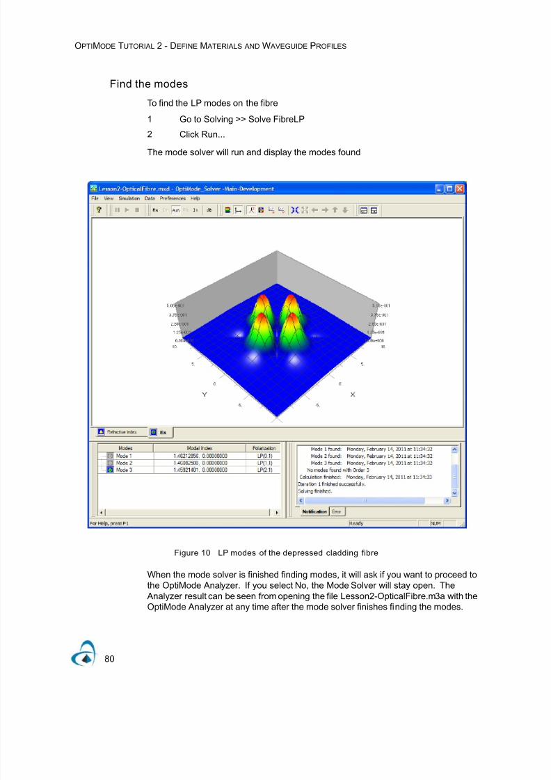
7/21/2019 OptiMode User Reference
http://slidepdf.com/reader/full/optimode-user-reference 84/339
OPTIMODE TUTORIAL 2 - DEFINE M ATERIALS AND W AVEGUIDE PROFILES
80
Find the modes
To find the LP modes on the fibre
1 Go to Solving >> Solve FibreLP
2 Click Run...
The mode solver will run and display the modes found
Figure 10 LP modes of the depressed cladding fibre
When the mode solver is finished finding modes, it will ask if you want to proceed tothe OptiMode Analyzer. If you select No, the Mode Solver will stay open. The
Analyzer result can be seen from opening the file Lesson2-OpticalFibre.m3a with theOptiMode Analyzer at any time after the mode solver finishes finding the modes.

7/21/2019 OptiMode User Reference
http://slidepdf.com/reader/full/optimode-user-reference 85/339
OPTIMODE TUTORIAL 2 - DEFINE M ATERIALS AND W AVEGUIDE PROFILES
81
In the OptiMode Solver, clicking on a mode in the Mode Found window will changethe main window to display the field pattern of that mode. Note that 3 modes wererequested for each of the Orders 0, 1, 2, and 3, but no more than one mode was foundfor each Order. In the case of Order 3, no modes could be found (there is a sentencein the Notification Window explaining this).
View Results in the OptiMode Analyzer
A permanent record of the mode solving session is made by the simulator. The filehas the same name as the OptiMode project with the file extension .m3a. To view therecord of this simulation
Open the OptiMode Analyzer from the Start Menu
Go to File >> Open, and navigate to the file Lesson2-OpticalFibre.m3a
The Analyzer has items under the Iteration heading with graphical display of refractiveindex distribution and modal index and field, similar to the mode solver. The modeindices are found in a combo box that select which mode field will be displayed. Thereis also a Solver Information Page, as shown in Figure 11.

7/21/2019 OptiMode User Reference
http://slidepdf.com/reader/full/optimode-user-reference 86/339
OPTIMODE TUTORIAL 2 - DEFINE M ATERIALS AND W AVEGUIDE PROFILES
82
Figure 11 The Solver Parameters page in the OptiMode Analyzer
The Solver Parameters heading records that these modes were found by the FibreLPmode solver, and what parameters were given for finding modes, as well as thewavelength. The next heading is User Parameters. Our example doesn’t have anyof these, but they will be introduced in the next tutorial, “OptiMode Tutorial 3 -Parameter Scanning” on page 83.

7/21/2019 OptiMode User Reference
http://slidepdf.com/reader/full/optimode-user-reference 87/339
OPTIMODE TUTORIAL 3 - P ARAMETER SCANNING
83
OptiMode Tutorial 3 - Parameter Scanning
This tutorial demonstrates User Parameters, scanning of parameters, and graphicaldisplay of scanned results. The analysis is done on the same structure as in theprevious tutorial, “OptiMode Tutorial 2 - Define Materials and Waveguide Profiles” onpage 71. In this tutorial, the effect of the width of the depressed cladding on modalindex will be investigated. To do this, User Parameters will be defined for the radiusof the fibre core and the width of the cladding. A sequence of dialog boxes thatarranges parameter scanning will be demonstrated, as well as how to requestgraphical display of the scanned results.
The starting point of this tutorial is the end of the previous tutorial. Open the finishedTutorial 2 project, and save it under a new name for this tutorial. Alternately, openOptiMode Cross Section Designer, navigate to the supplied sample Lesson2-OpticalFibre.mxd, open that and save it under a new name.
Define User Parameters
User Parameters are defined in the Variables and Functions dialog box. This box isopened from Solving >> Edit Parameters... , or from clicking on any field that has thefx on the left side of the field. This project will define two User Parameters, one forthe radius of the fibre core and the other for the thickness of the depressed cladding.
3 Go to Solving >> Edit Parameters...
4 In the User Variables tab, enter the name “core_radius” in the Name field
5 Enter 4.0 in the Expression field
6 Click Verify
7 Click Add/Apply
The new User Parameter will appear in the User Variables tab in the lower panel ofthe box, as in Figure 1

7/21/2019 OptiMode User Reference
http://slidepdf.com/reader/full/optimode-user-reference 88/339
OPTIMODE TUTORIAL 3 - P ARAMETER SCANNING
84
Figure 1 The Variables and Functions dialog box
1 Repeat steps 2 to 5 to add another User Parameter, the width of thedepressed cladding, “width_dc”.
2 Set value of width_dc to 1.
These parameters are globally defined in the project. Sometimes it is worth definingthem if the parameter is used in many places. All instances of the parameter can bechanged by applying a new value once in the Variables and Functions dialog box. Inthis tutorial, the parameter definition is used to scan the value according to a scheduledefined in the Parameter Sweep Definition dialog box.
The core radius and width of depressed clad layer are used in the profile definitionand the width of the waveguide in the layout. To put the parameters in the profiledefinition
1 Go to Edit >> Profiles and Materials to open the Profile Designer
2 Double click on FiberPro1 to open the Profile definition in the main window
3 Select Layer 1 in the layer list
4 Write “core_radius” in the Rx and Ry fields
5 Click Apply
After this, update the second layer radius with a radius of “core_radius + width_dc”(one can write expressions as well as parameters in the fx fields)

7/21/2019 OptiMode User Reference
http://slidepdf.com/reader/full/optimode-user-reference 89/339
OPTIMODE TUTORIAL 3 - P ARAMETER SCANNING
85
1 Select Layer 2 in the layer list
2 Write “core_radius + width_dc” in the Rx and Ry fields
3 Click Apply
4 Click Store
The FiberPro1 profile will have layer widths defined by the User Parameters as inFigure 2.
Figure 2 Parameterized layer width definitions for the fiber profile
The actual size of the optical fibre is determined by the width of the waveguide in thelayout. We will set this width to 2 (core_radius + width_dc), so that the fibre has coreand cladding according to the numerical value of the parameters. (If the waveguidewidth is another value, the Rx and Ry values determine only the ratio of layer widths).

7/21/2019 OptiMode User Reference
http://slidepdf.com/reader/full/optimode-user-reference 90/339
OPTIMODE TUTORIAL 3 - P ARAMETER SCANNING
86
To set the waveguide width,
1 Double click on the waveguide in the Layout Properties window to open theXS Linear Waveguide Properties dialog box
2 In the width field, write 2 * (core_radius + width_dc), as in Figure 3.
3 Click OK
Figure 3 Parameterized Waveguide Properties
Note that changing the core_radius or width_dc parameter will make the Layout andrefractive index distribution change accordingly.
Define a parameter sweep
OptiMode can be made to perform many simulations with various values of the UserParameters. Use this feature if you want to understand how your structure changeswith changes in geometry or material parameters.
1 Go to Tools >> Parameter Sweep to open the Parameter Sweep Definitiondialog box
2 Click on Parameters to open the Parameter Selection dialog box. Allparameters defined in the project are displayed in this box
3 Select the parameter width_dc and click OK
The Parameter Sweep Definition dialog box now has the parameter width_dc listedunder Level 1
1 Right click on Level1
2 Select Set Iteration Count
3 Set the iteration number to 11
4 Click OK
The Parameter Sweep Definition dialog box should appear as in Figure 4.

7/21/2019 OptiMode User Reference
http://slidepdf.com/reader/full/optimode-user-reference 91/339
OPTIMODE TUTORIAL 3 - P ARAMETER SCANNING
87
Figure 4 the Parameter Sweep Definition dialog box
The box indicates the simulation will be performed 11 times, and the value of width_dcwill be according to the table for each iteration. Each number in the list can be editedin this dialog box, and the number will be used in the simulation. There are SpreadTools in the lower right to assign values automatically. To use the Linear Tool
1 Click on the width_dc at the top of the column of iterations. This will selectthe whole column.
2 Click on the Linear button. This will open the Parameter Iteration Spreaddialog box
3 Enter 0.0 as the start value, and 5.0 as the end value
4 Click OK
The values for width_dc will now be 0, 0.5, 1.0, 1.5, and so on up to 5.0 in a linearsequence.
Specify Graphical Output
If this project is run with this parameter sweep definition, the mode solver will be called11 times, with the parameter width_dc set according to the list in the ParameterSweep Definition dialog box. All results are sent to the same Analyzer file, and theresult of each iteration is selected for viewing by using the Iteration combo box.OptiMode can also display the modal index in the form of a graph, with the parameteron the x axis. To request a graph like this

7/21/2019 OptiMode User Reference
http://slidepdf.com/reader/full/optimode-user-reference 92/339
OPTIMODE TUTORIAL 3 - P ARAMETER SCANNING
88
1 In the Parameter Sweep Definition dialog box, click Graphs...
2 In the User Defined Graphs dialog box, click Add to add a graph to get the Add/Edit dialog box
3 Enter Modal Index for the Graph Title
4 Enter n for the Y axis title
5 For Y axis values, select Modal Index
6 Enter dc thickness for the x axis title
7 Select Mode Data - Polarization for the Legend
8 Click OK
9 Click OK
10 Click OK to return to the OptiMode XS Designer
Run a Sweep
Now run the project by going to Solving >> Solve FibreLP. The dialog box displayedbefore running is shown in Figure 5.
Figure 5 the Solver Parameters dialog box.
Note that the check box Use Sweep Script has been selected. This is done
automatically by OptiMode when a parameter sweep is defined. If you don’t want torun the sweep, unselect this check box, and one simulation will be done with UserParameters as currently defined in the Variables and Functions dialog box.
During the running you’ll see the mode solver go through the 11 iterations, and theresults will scroll past in the Mode Found window. Open the Analyzer when asked.
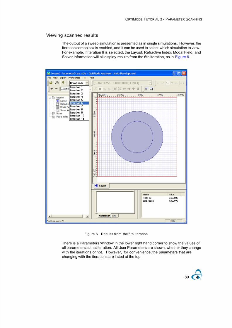
7/21/2019 OptiMode User Reference
http://slidepdf.com/reader/full/optimode-user-reference 93/339
OPTIMODE TUTORIAL 3 - P ARAMETER SCANNING
89
Viewing scanned results
The output of a sweep simulation is presented as in single simulations. However, theIteration combo box is enabled, and it can be used to select which simulation to view.For example, if Iteration 6 is selected, the Layout, Refractive Index, Modal Field, and
Solver Information will all display results from the 6th iteration, as in Figure 6.
Figure 6 Results from the 6th iteration
There is a Parameters Window in the lower right hand corner to show the values ofall parameters at that iteration. All User Parameters are shown, whether they changewith the iterations or not. However, for convenience, the parameters that arechanging with the iterations are listed at the top.

7/21/2019 OptiMode User Reference
http://slidepdf.com/reader/full/optimode-user-reference 94/339
OPTIMODE TUTORIAL 3 - P ARAMETER SCANNING
90
There is a new item on the navigator pane, the Modal Index graph we requested asgraphical output. It is independent of iterations and found at the bottom of the list.
1 Select Modal Index, the graph will appear in the main window.
2 In the graph, right click and select Legend. This should appear as in Figure 7
Figure 7 Graphical output of parameter sweep
The graph shows the modal index of all the modes as a function of the thickness ofthe depressed cladding layer. It seems to affect the higher order modes more stronglythan the fundamental mode, and the increased thickness causes the highest mode,LP(0,2), to cut-off.

7/21/2019 OptiMode User Reference
http://slidepdf.com/reader/full/optimode-user-reference 95/339
OPTIMODE TUTORIAL 4 - MULTI-LEVEL SCANNING
91
OptiMode Tutorial 4 - Multi-level Scanning
This tutorial demonstrates scanning of parameters on two levels and graphical displayusing a Legend.
The starting point of this tutorial is the end of the previous tutorial. Open the finishedTutorial 3 project, and save it under a new name for this tutorial. Alternately, openOptiMode Cross Section Designer, navigate to the supplied sample Lesson3-OpticalFibre.mxd, open that and save it under a new name to start this tutorial.
At a longer wavelength, 1.3 , the depressed cladding fibre of this sample isusually single mode. In this tutorial the influence of the cladding thickness on thefundamental modal index will be investigated. At the same time, the simulation willbe done for different values of core radius. The graphical presentation of results willclearly show the relevant trend.
Set the wavelength
The first step is to change the wavelength of the project:
Go to Solving >> Solver Parameters, and change the wavelength to 1.3 , as inFigure 1.
Figure 1 set the wavelength to 1.3
Specify a two-level scan of User Parameters
The simulation will sweep through the same range of thickness of cladding layer asbefore. However, the radius of the core parameter will be included.
μm
μm
μm

7/21/2019 OptiMode User Reference
http://slidepdf.com/reader/full/optimode-user-reference 96/339
OPTIMODE TUTORIAL 4 - MULTI-LEVEL SCANNING
92
3 Go to Tools >> Parameter Sweep
4 Click Parameters...
5 Select core_radius (as well as width_dc)
6 Click OK
7 In the Parameter Sweep dialog box, select Level1. It should look like Figure 2
Figure 2 More than one User Parameter in the sweep
The two selected User Parameters are shown with their current values and the defaultnumber of iterations. The desired number of iterations can be set, and the value ofeach parameter can be defined as already described in Tutorial 3.
In this tutorial, we show how to arrange a two level parameter scan, where theparameter on the lower level sweeps through the whole range while the upper levelparameters are held constant. The upper level parameter is then changed to the nextvalue on its list, and the lower level parameters are swept through their ranges again.
In the special case of two-level scan, it is possible to arrange graphical output with the
higher level parameter in the legend of the graph. This tutorial will show how tospecify a multi-level scan with that kind of graphical display.

7/21/2019 OptiMode User Reference
http://slidepdf.com/reader/full/optimode-user-reference 97/339
OPTIMODE TUTORIAL 4 - MULTI-LEVEL SCANNING
93
Create parameter levels
1 In the Parameter Sweep Definition dialog box, Right click on Level 1 andselect Add Level. The two parameters will now be found under Level 2
2 Drag and drop the core_radius parameter under Level 1, so that width_dc is
under Level 2, and core_radius is under Level 1.3 Right click on Level 1, and set the Iteration Count to 3.
4 Select core_radius column and click Linear...
5 In the Parameter Iteration Spread dialog box set the start value to 3 and theend to 5, as in Figure 3
Figure 3 Level 1 of the multi -level sweep

7/21/2019 OptiMode User Reference
http://slidepdf.com/reader/full/optimode-user-reference 98/339
OPTIMODE TUTORIAL 4 - MULTI-LEVEL SCANNING
94
6 Select Level 2, and repeat steps 3, 4, and 5, but make the Iteration Count 11and make the range of width_dc go from 0 to 5, as in Figure 4
Figure 4 Level 2 of the multi -level sweep
With the Parameter Sweep dialog box in this condition, OptiMode will start thesimulator with core_radius = 3, and will run 11 simulations for all values of width_dcfrom 0 to 5. Then it will set core_radius = 4, and will run another 11 simulations for allthe width_dc values. Finally, it will set core_radius = 5, and find all modes for all thewidth_dc values. All 33 iterations can be reviewed in the Analyzer, and the values ofwidth_dc and core_radius are displayed in the Parameters Window for each iteration.
Specify a graphical display with legend
The kind of two-level sweep is best displayed as a graph with the Level 2 parameteron the X axis and the Level 1 parameter in the legend. To do this
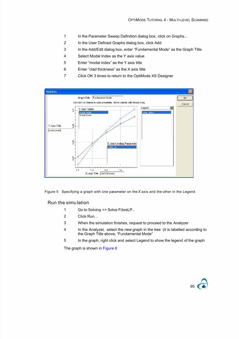
7/21/2019 OptiMode User Reference
http://slidepdf.com/reader/full/optimode-user-reference 99/339
OPTIMODE TUTORIAL 4 - MULTI-LEVEL SCANNING
95
1 In the Parameter Sweep Definition dialog box, click on Graphs...
2 In the User Defined Graphs dialog box, click Add
3 In the Add/Edit dialog box, enter “Fundamental Mode” as the Graph Title
4 Select Modal Index as the Y axis value
5 Enter “modal index” as the Y axis title
6 Enter “clad thickness” as the X axis title
7 Click OK 3 times to return to the OptiMode XS Designer
Figure 5 Specifying a graph with one parameter on the X axis and the other in the Legend
Run the simulation
1 Go to Solving >> Solve FibreLP...
2 Click Run...
3 When the simulation finishes, request to proceed to the Analyzer
4 In the Analyzer, select the new graph in the tree (it is labelled according tothe Graph Title above, “Fundamental Mode”
5 In the graph, right click and select Legend to show the legend of the graph
The graph is shown in Figure 6

7/21/2019 OptiMode User Reference
http://slidepdf.com/reader/full/optimode-user-reference 100/339
OPTIMODE TUTORIAL 4 - MULTI-LEVEL SCANNING
96
Figure 6 Graphical output wit h one parameter on the X axis and the other in the Legend
This graph shows the same decrease in modal index with increasing depressedcladding thickness as seen in the previous tutorial. It also shows that this effect ismore pronounced if the fibre core radius is reduced.
Specify more than one graph
It is possible to request more than one graph for display in the Analyzer. Other datamay be of interest, for example, it happens that not all combinations of fibres with
core_radius and width_dc in this simulation are single mode. Some have a secondmode. To see this, one can request another graph with the same X axis and Legend,but with number of modes found in the Y axis (instead of fundamental mode index).To do this

7/21/2019 OptiMode User Reference
http://slidepdf.com/reader/full/optimode-user-reference 101/339
OPTIMODE TUTORIAL 4 - MULTI-LEVEL SCANNING
97
1 Go to Tools >> Parameter Sweep
2 In the Parameter Sweep Definition dialog box, click on Graphs...
3 In the User Defined Graphs dialog box, click Add
4 In the Add/Edit dialog box, enter Mode Count as the title
5 Enter “number of modes” as the Y axis title
6 Select Mode Count as the Y axis Value
7 Enter “clad thickness” as the X axis title
Figure 7 graph of number of modes
8 Click OK 3 times to return to the OptiMode XS Designer
9 Go to Solving >> Solve FibreLP...
10 Click Run...
11 After the Analyzer loads, select the Mode Count graph.
12 In the graph, right click and select Legend
In the resulting graph of Mode Count (Figure 8), we can see the fibre is a single mode
waveguide except for the cases core_radius = 5 and width_dc = 0 or 0.5.

7/21/2019 OptiMode User Reference
http://slidepdf.com/reader/full/optimode-user-reference 102/339
OPTIMODE TUTORIAL 4 - MULTI-LEVEL SCANNING
98
Figure 8 Number of modes found in each simulation

7/21/2019 OptiMode User Reference
http://slidepdf.com/reader/full/optimode-user-reference 103/339
OPTIMODE TUTORIAL 5 - PHOTONIC CRYSTAL FIBRE AND VB SCRIPT
99
OptiMode Tutorial 5 - Photonic Crystal Fibre andVB Script
In this tutorial, we make the hexagonal crystal lattice fibre of Reference 1. Thephotonic crystal fibre consists of an array of holes parallel to the fibre axis. In thisproblem the material of substrate and cladding will be set to the glass of the fibre. TheFibre Profile, defined with a single layer of air as the material, can be used to definea circular hole in the fibre. One can place as many holes as needed to make the arrayof the photonic crystal fibre. Although it is possible to do this by hand, the job is rathertedious. OptiMode has a VB Script that can be used for automatic placement of theholes. This tutorial will introduce the script and show how it can be used to constructthe photonic crystal fibres of Reference [3].
Define Materials and Profile
The photonic crystal fibre needs only two materials and one profile. One material is Air (for the holes), and the other is the glass of the fibre.
13 Go to File >> New to start a new project
14 Click on Profiles and Materials to open the Profile Designer
15 Create the glass material. Call it “SiO2” and set its refractive index to 1.45.
16 The Profile is a Fiber Profile. Call it “Hole” and make it one layer of Air, withsemi-radii Rx = 1 and Ry = 1. (Figure 1)
The Rx and Ry serve only to define the relative semi-axes. The actual diameter ofthe hole will be the width of the waveguide in the layout, not yet defined.

7/21/2019 OptiMode User Reference
http://slidepdf.com/reader/full/optimode-user-reference 104/339
OPTIMODE TUTORIAL 5 - PHOTONIC CRYSTAL FIBRE AND VB SCRIPT
100
Figure 1 Material and Profile definitions. This profile will make a circular hole.

7/21/2019 OptiMode User Reference
http://slidepdf.com/reader/full/optimode-user-reference 105/339
OPTIMODE TUTORIAL 5 - PHOTONIC CRYSTAL FIBRE AND VB SCRIPT
101
1 In the Initial Properties dialog box, set the Default Width to 1.0, and theDefault Waveguide to Hole.
2 In the 3D Wafer Properties tab, Set the width to 25
3 Set both Cladding and Substrate materials to SiO2, and their widths to 12
(Figure 2)4 Save the project.
Figure 2 Initial Properties
1 Click on the waveguide item to put a new circular waveguide in the Layout.
2 Drag and drop the waveguide to some random place.
3 Repeat two or three times to get a few waveguides scattered through theLayout, as in Figure 3

7/21/2019 OptiMode User Reference
http://slidepdf.com/reader/full/optimode-user-reference 106/339
OPTIMODE TUTORIAL 5 - PHOTONIC CRYSTAL FIBRE AND VB SCRIPT
102
Figure 3 Layout with 3 holes

7/21/2019 OptiMode User Reference
http://slidepdf.com/reader/full/optimode-user-reference 107/339
OPTIMODE TUTORIAL 5 - PHOTONIC CRYSTAL FIBRE AND VB SCRIPT
103
Use Generate Layout Script ...
1 Click on the Scripting tab. (It should be empty.)
2 Go to Tools >> Generate Layout Script...
3 The dialog box will warn about overwriting any script that is currently there.Click Yes.
The following text will appear in the Scripting tab
WGMgr.DeleteAll
Dim WGCrossSection1
Set WGCrossSection1 = WGMgr.CreateObj ( "WGLinearXS",
"WGCrossSection1" )
WGCrossSection1.SetStart -5.55, 2.85
WGCrossSection1.SetAttr "WidthExpr", "1"
WGCrossSection1.SetProfileName "Hole"
Dim WGCrossSection2
Set WGCrossSection2 = WGMgr.CreateObj ( "WGLinearXS",
"WGCrossSection2" )
WGCrossSection2.SetStart 4.2, 4.85
WGCrossSection2.SetAttr "WidthExpr", "1"
WGCrossSection2.SetProfileName "Hole"
Dim WGCrossSection3
Set WGCrossSection3 = WGMgr.CreateObj ( "WGLinearXS",
"WGCrossSection3" )
WGCrossSection3.SetStart 2.3, -3.55
WGCrossSection3.SetAttr "WidthExpr", "1"
WGCrossSection3.SetProfileName "Hole"
To see the function of this script, do the following1 Return to the Layout page
2 Select the waveguides in the Layout and delete them all
3 Go to Tools >> Run Script
The waveguides will re-appear. The new waveguides have been created by thescript. The script can be used to create waveguides and arrange them in the Layout.

7/21/2019 OptiMode User Reference
http://slidepdf.com/reader/full/optimode-user-reference 108/339
OPTIMODE TUTORIAL 5 - PHOTONIC CRYSTAL FIBRE AND VB SCRIPT
104
In this script, note there are 3 paragraphs, one for each object in the layout. The firstline defines a variable in VB. In the second line, the variable is made into an objectby the Set command. This is done by the OptiMode supplied structure WGMgr, whichhas a function named CreateObj that will create a new object in the layout. The firstargument of the function, “WGLinearXS”, indicates that the new layout object should
be a waveguide (instead of a Substrate Layers or a user defined refractive indexdistribution). The second argument gives the new waveguide a unique name. Thatis the name that appears in the Label field of the XS Linear Waveguide Propertiesdialog box for that waveguide. The third line positions the waveguide in the X, Yplane. (If those numbers are changed, an the script run again, the waveguides in thelayout will move to the new location). The fourth line sets the width of the waveguideto 1.0, and the last line specifies which Profile should be used to define thiswaveguide’s cross section profile.
Write your own script
The environment in which these lines are written is a VB Script environment, soanything that can be done in VB Script can be done here by writing the appropriate
code. For example, instead of creating three waveguides by writing threeparagraphs, the three could be made from a single paragraph that is contained in aVB For - Next loop. There are, however, two things that should change for eachiteration of the loop. One is the name of the new waveguide, since each waveguidemust have a unique name. The other is the position. There isn’t much point increating three identical waveguides in the same place. To create a unique name, thestring concatenation feature of VB can be used. A name can be given as a prefix, andthe suffix, added by string concatenation, can be made up from the loop countingindex, as in the script below.
'Make waveguides in a loop
Option Explicit ' do not permit variables that have not been declared
WGMgr.DeleteAll ' delete all waveguides currently in the layout
Dim loop_index, waveguide_object, hole_diameter, x_coord, waveguide_name
hole_diameter = 5
For loop_index = 1 To 3
'unique name for the new waveguide "HoleNumber_x" ( x = 1, 2, or 3)
waveguide_name = "HoleNumber_" & CStr( loop_index)
Set waveguide_object = WGMgr.CreateObj("WGLinearXS", waveguide_name)
x_coord = - 12 + 6 * loop_index
waveguide_object.SetStart x_coord, 0.0 MsgBox("WG name is " & waveguide_name & ", WG position is "_&
CStr(x_coord) )
waveguide_object.SetAttr "WidthExpr", CStr( hole_diameter)
waveguide_object.SetProfileName "Hole"
Next

7/21/2019 OptiMode User Reference
http://slidepdf.com/reader/full/optimode-user-reference 109/339
OPTIMODE TUTORIAL 5 - PHOTONIC CRYSTAL FIBRE AND VB SCRIPT
105
The apostrophe makes comments of any characters following it. Option Explicit is a
good idea, it will prevent the confusion that results when a variable is miss-spelt by
mistake. CStr( ) is a standard VB function that takes a numerical variable and
converts it to a string. Some of the of the functions used need strings in their
arguments, even though the data being passed are numbers. The MsgBox commandis useful for checking the program is running as expected, but later you might want to
make it a comment so it won’t stop the execution. The underscore at the end of the
MsgBox line permits the command definition to be continued on the next line. After
running the script, the Layout should appear as in Figure 4.
Figure 4 Layout after running the Make waveguides in a loop script.
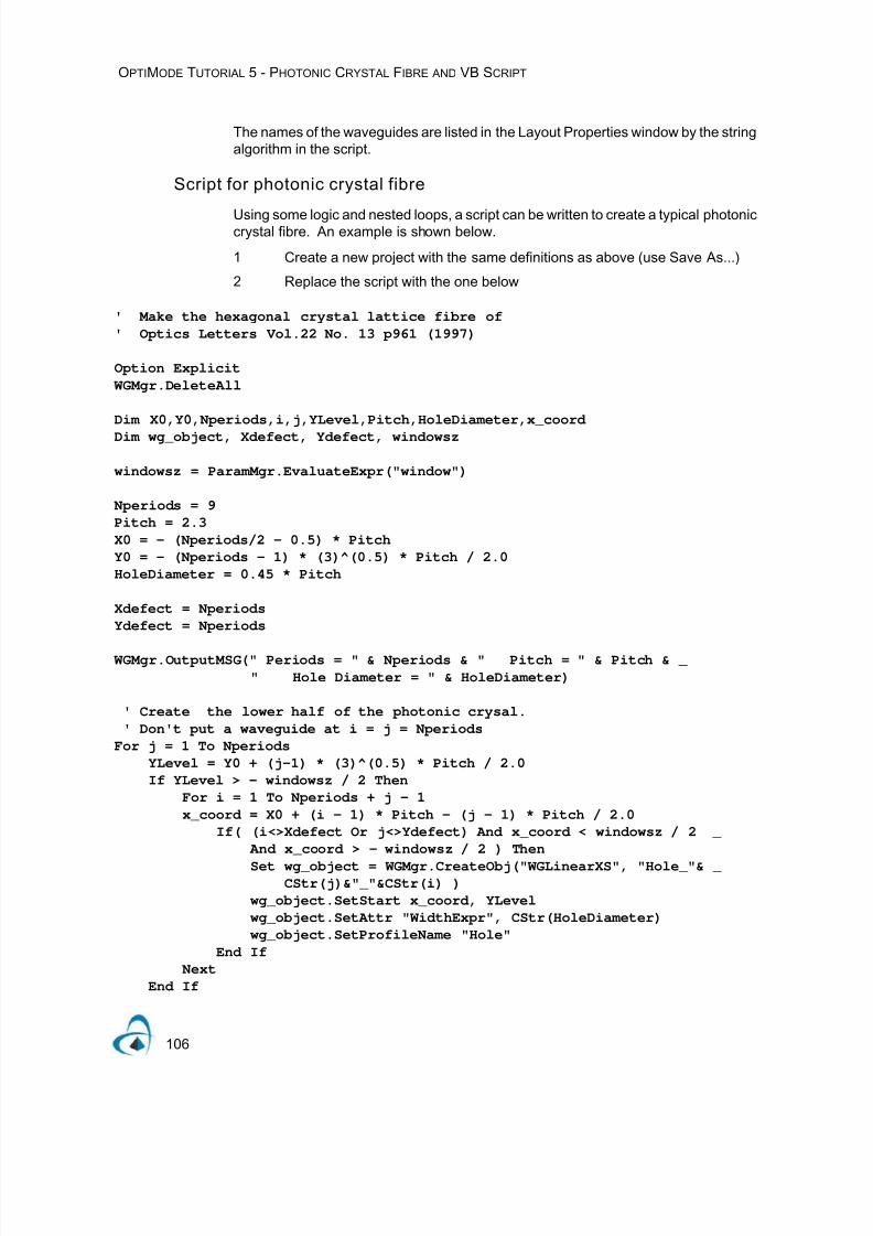
7/21/2019 OptiMode User Reference
http://slidepdf.com/reader/full/optimode-user-reference 110/339
OPTIMODE TUTORIAL 5 - PHOTONIC CRYSTAL FIBRE AND VB SCRIPT
106
The names of the waveguides are listed in the Layout Properties window by the stringalgorithm in the script.
Script for photonic crystal fibre
Using some logic and nested loops, a script can be written to create a typical photoniccrystal fibre. An example is shown below.
1 Create a new project with the same definitions as above (use Save As...)
2 Replace the script with the one below
' Make the hexagonal crystal lattice fibre of
' Optics Letters Vol.22 No. 13 p961 (1997)
Option Explicit
WGMgr.DeleteAll
Dim X0,Y0,Nperiods,i,j,YLevel,Pitch,HoleDiameter,x_coord
Dim wg_object, Xdefect, Ydefect, windowsz
windowsz = ParamMgr.EvaluateExpr("window")
Nperiods = 9
Pitch = 2.3
X0 = - (Nperiods/2 - 0.5) * Pitch
Y0 = - (Nperiods - 1) * (3)^(0.5) * Pitch / 2.0
HoleDiameter = 0.45 * Pitch
Xdefect = Nperiods
Ydefect = Nperiods
WGMgr.OutputMSG(" Periods = " & Nperiods & " Pitch = " & Pitch & _
" Hole Diameter = " & HoleDiameter)
' Create the lower half of the photonic crysal.
' Don't put a waveguide at i = j = Nperiods
For j = 1 To Nperiods
YLevel = Y0 + (j-1) * (3)^(0.5) * Pitch / 2.0
If YLevel > - windowsz / 2 Then
For i = 1 To Nperiods + j - 1
x_coord = X0 + (i - 1) * Pitch - (j - 1) * Pitch / 2.0
If( (i<>Xdefect Or j<>Ydefect) And x_coord < windowsz / 2 _
And x_coord > - windowsz / 2 ) Then
Set wg_object = WGMgr.CreateObj("WGLinearXS", "Hole_"& _CStr(j)&"_"&CStr(i) )
wg_object.SetStart x_coord, YLevel
wg_object.SetAttr "WidthExpr", CStr(HoleDiameter)
wg_object.SetProfileName "Hole"
End If
Next
End If

7/21/2019 OptiMode User Reference
http://slidepdf.com/reader/full/optimode-user-reference 111/339
OPTIMODE TUTORIAL 5 - PHOTONIC CRYSTAL FIBRE AND VB SCRIPT
107
Next
' Create the upper half of the photonic crystal
For j = Nperiods + 1 To 2 * Nperiods - 1
YLevel = Y0 + (j-1) * (3)^(0.5) * Pitch / 2.0
If YLevel < windowsz / 2 ThenFor i = 1 To 3 * Nperiods - j - 1
x_coord = X0 + (i - 1) * Pitch + (j - 2 * Nperiods + 1) _
* Pitch / 2.0
If x_coord < windowsz / 2 And x_coord > - windowsz / 2 Then
Set wg_object = WGMgr.CreateObj("WGLinearXS", "Hole_" _
&CStr(j) &"_"&CStr(i) )
wg_object.SetStart x_coord, YLevel
wg_object.SetAttr "WidthExpr", CStr(HoleDiameter)
wg_object.SetProfileName "Hole"
End If
NextEnd If
Next
When this script is run, the layout creates a photonic crystal lattice as shown in Figure5.
Figure 5 Photonic crys tal fibre of Ref. 1
7/21/2019 OptiMode User Reference
http://slidepdf.com/reader/full/optimode-user-reference 112/339
OPTIMODE TUTORIAL 5 - PHOTONIC CRYSTAL FIBRE AND VB SCRIPT
108
Finding modes of photonic crystals
To find the mode of a photonic crystal fibre, several settings are required. The meshneeds to be quite fine. The mode is always lossy, only complex modes exist, so theComplex mode solver must be called, (not the real one). The boundary condition
should allow the losses, so it should be set to TBC (Transparent Boundary Condition).The waveguide has high index contrast, so a full vector solution is the most accurate.The ADI mode solver needs a Gaussian field as an initial guess of the mode. Formost waveguides, this is based on the waveguide dimensions, and the waveguideused is marked with a G in the Waveguide Properties window. However, this is not agood choice for photonic crystals, since the mode is not likely to be centred on one ofthe holes. As a result, it is better to specify the starting field manually. To make thesesettings for this example
1 Go to Solving >> Solver parameters >> ADI tab
2 In Solver panel, select Complex
3 In Mode Panel, select Full Vector Initial Excitation along X
4 Number of points in Mesh = 350 in X an Y5 Number of Modes = 1
6 Wavelength = 1.55
In the Settings tab
1 Click Properties in the Starting Field panel
2 Select type User Defined
3 For the Center Point enter X = 0 and Y = 0
4 For Width, enter Halfwidth X = 1 and Halfwidth Y = 1
5 Click OK
6 Click OK
Then start the mode solver from Solving >> Solve ADI >> Run ... The result shouldbe as in Figure 6.

7/21/2019 OptiMode User Reference
http://slidepdf.com/reader/full/optimode-user-reference 113/339
OPTIMODE TUTORIAL 5 - PHOTONIC CRYSTAL FIBRE AND VB SCRIPT
109
Figure 6 Photonic Crystal mode for fibre of Ref. 1
References
[3] T.A. Birks, J.C. Knight, P. St. J. Russell, “Endlessly single-mode photonic crystal fiber”, OpticsLetters Vol.22 No. 13 p961-963 (1997)

7/21/2019 OptiMode User Reference
http://slidepdf.com/reader/full/optimode-user-reference 114/339
OPTIMODE TUTORIAL 5 - PHOTONIC CRYSTAL FIBRE AND VB SCRIPT
110

7/21/2019 OptiMode User Reference
http://slidepdf.com/reader/full/optimode-user-reference 115/339
OPTIMODE XS L AYOUT DESIGNER
111
OptiMode XS Layout Designer
When you create a new project in OptiMode XS Layout Designer, the followingwindow appears.
Figure 1 OptiMode Project Layout Window
Main parts of the GUI
The OptiMode Layout Designer GUI contains six main windows:
• Layout window
• Layout Designer dialog
• Ref Index
• Scripting
• Notes
• Output

7/21/2019 OptiMode User Reference
http://slidepdf.com/reader/full/optimode-user-reference 116/339
OPTIMODE XS L AYOUT DESIGNER
112
Layout Window
Figure 2 Layout window is a schematic view of the transverse plane
The Layout window is a schematic view of the transverse plane. The cross sectionsof the waveguides are shown as their exact ideal shapes. This is in contrast to theRefractive Index view, where the view shows the refractive index after application ofthe calculation mesh. In the Layout view, all shapes can be moved by mouse, and therelevant dialog boxes for properties can be opened as well.
Layout Designer Dialog
Figure 3 Layout Desinger Window
This dialog is used to edit the cross section layout and its components.
Refractive Index window
The Refractive Index window displays the refractive index of the main layout.

7/21/2019 OptiMode User Reference
http://slidepdf.com/reader/full/optimode-user-reference 117/339
OPTIMODE XS L AYOUT DESIGNER
113
Figure 4 Refractive Index disp lay
Scripting window
The Scripting window displays the Visual Basic script code to be used in the project.
Figure 5 Scripting Window
Notes window
Write important notes that you can refer to at any time. You can write the notes in anyformat, and they are saved with the layout. The notes you write in the Notes windowappear in the Open dialog box when you select the project file.

7/21/2019 OptiMode User Reference
http://slidepdf.com/reader/full/optimode-user-reference 118/339
OPTIMODE XS L AYOUT DESIGNER
114
Figure 6 Notes Window
Output window
The Output window can be moved around from its original location. The Notification
and Error tabs are there as tools to display any notifications or errors that may occurin the application. The Error tab is only for layout objects.
Figure 7 Output Window

7/21/2019 OptiMode User Reference
http://slidepdf.com/reader/full/optimode-user-reference 119/339
OPTIMODE XS L AYOUT DESIGNER
115
Main menu bar
The Main menu bar contains the menus that are available in OptiMode LayoutDesigner. Many of these menu items are also available as buttons on the toolbars.
Figure 8 Main Menu bar
Toolbars
Select the toolbars that you want to have availble in the main layout window.
File
Contains the buttons to perform all typicalwindows application actions. Available in
all views.
Scripting
Available in all views.
3D Graph
Only available in the Ref Index 2D XZ
Plane view.
Ref Idx. View Type
Only availale in the Ref Index view.
Tools
Only available in layout view.
Zoom
Only available in layout view.

7/21/2019 OptiMode User Reference
http://slidepdf.com/reader/full/optimode-user-reference 120/339
OPTIMODE XS L AYOUT DESIGNER
116

7/21/2019 OptiMode User Reference
http://slidepdf.com/reader/full/optimode-user-reference 121/339
OPTIMODE L AYOUT DESIGNER MENUS AND BUTTONS
117
OptiMode Layout Designer menus and buttons
This section describes the menus and buttons available in OptiMode LayoutDesigner.
File menu
File menu item Toolbar
button
Description
New (Ctrl+N)Create a new project. When a new project is created, the Initial Properties dialogbox appears.
Open (Ctrl+O)Opens an existing project. Select the project from the Open dialog box.
Close — Closes the active project. You are prompted to save changes.
Save (Ctrl+S)Saves the active project under the current name in the default location.
Save As —
Saves the current project with a different name and in a location that you select.
The SaveAs dialog box contains a special feature that allows you to write a quick
memo about the file for future reference.
Print (Ctrl+P)Prints the active project.
Print Preview — Displays how the printed page will appear.
Print Setup — Allows you to set up the printer, page size, orientation, and allows you to set otherprinting options.
Recent files — Lists the most recent files that you worked on.
Exit — Closes OptiMode Layout Designer .
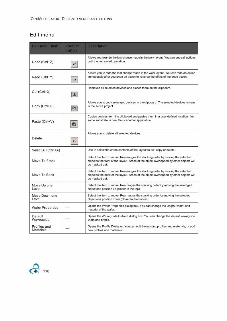
7/21/2019 OptiMode User Reference
http://slidepdf.com/reader/full/optimode-user-reference 122/339
OPTIMODE L AYOUT DESIGNER MENUS AND BUTTONS
118
Edit menu
Edit menu item Toolbar
button
Description
Undo (Ctrl+Z)
Allows you to undo the last change made in the work layout. You can undo all actions
until the last saved opetation.
Redo (Ctrl+Y)
Allows you to redo the last change made in the work layout. You can redo an action
immediately after you undo an action to reverse the effect of the undo action.
Cut (Ctrl+X)
Removes all selected devices and places them on the clipboard.
Copy (Ctrl+C) Allows you to copy selectged devices to the clipboard. The selected devices remainin the active project.
Paste (Ctrl+V)
Copies devices from the clipboard and pastes them in a user-defined location_the
same substrate, a new file or another application.
Delete
Allows you to delete all selected devices.
Select Al l (Ctrl+A) Use to select the entire contents of the layout to cut, copy or delete.
Move To FrontSelect the item to move. Reaaranges the stacking order by moving the selected
object to the front of the layout. Areas of the object overlapped by other objects willbe masked out.
Move To BackSelect the item to move. Reaaranges the stacking order by moving the selected
object to the back of the layout. Areas of the object overlapped by other objects will
be masked out.
Move Up oneLevel
Select the item to move. Rearranges the stacking order by moving the selectged
object one position up (closer to the top).
Move Down oneLevel
Select the item to move. Rearranges the stacking order by moving the selected
object one position down (closer to the bottom).
Wafer Properties —Opens the Wafer Properties dialog box. You can change the length, width, and
material of the wafer.
DefaultWaveguide
—Opens the Waveguide Default dialog box. You can change the default waveguide
width and profile.
Profiles andMaterials
—Opens the Profile Designer. You can edit the existing profiles and materials, or add
new profiles and materials.

7/21/2019 OptiMode User Reference
http://slidepdf.com/reader/full/optimode-user-reference 123/339
OPTIMODE L AYOUT DESIGNER MENUS AND BUTTONS
119
View menu
View menu i tem Too lbar
button
Description
Toolbars — For more information, see “Toolbars” on page 115. When you select a toolbar, a
check mark appears next to the name of the toolbar in the Toolbars menu.
Status Bar — Select to display the Status Bar. Displays the coordinates of the cursor position.
Output Window — Select to display the Output Window. Displays notification and error messages
regarding the script.
Color Spectrum —Select to display the Color Spectrum. Displays the colors available for thewaveguides in the layout. By default the COlor Spectrum is selected.
Workbook Mode — Allows you to switch between open layout files using the Tab key. If you do notchoose this method for switching between files, use the windows menu.
3D Graph Items
PaletteToggles the Visualizer Palette on or off.
AxisToggles the Axis on or off.
Height Plot
This button will toggle to the 3D view. If this button is selected, the Plane view and
Visualizer button will be disabled.
For each data element in the data array (matrix), there is a (x,y,z) point. The x value
= data element’s column index to x (horizontal position), its row index = y (verticalposition), and its data elements value = z (refractive index value). Depending on the
current GraphStyle (Height Plot Settings), these points may be displayed as
individual points, or connected to form either lines or a surface.
Image Map
For each data element in the matrix, there is a (x,y) point. The x value = dataelement’s column index, the y value = row index, and the color is based on thecurrent color Palette. The collection of points is drawn as a 2D image.
Note: For the Avis2D toolbar to be activated, the Refractive Index tab must be
selected. This can also be found under the View menu, in case this toolbar is notdisplayed.
Plane View (XZ)Toggles the (XZ) view on or off.
Plane View (YZ)Toggles the (YZ) view on or off.
Zoom InIncreases the image in the layout by 1.00000 times for the first ten clicks.
Zoom OutDecreases the image in the layout by 1.00000 times for each click.
Pan LeftIs available only if the Zoom In option has been activated. The Pan Left command
moves the selected area to the left.

7/21/2019 OptiMode User Reference
http://slidepdf.com/reader/full/optimode-user-reference 124/339
OPTIMODE L AYOUT DESIGNER MENUS AND BUTTONS
120
Pan RightMoves the selected area to the right.
Pan UpMoves the selected area upwards.
Pan DownMoves the selected area downwards.
Refractive Index Data Type
RealOptical field described by real numbers.
ImaginaryOptical field described by imaginary numbers.
View menu i tem Too lbar
button
Description

7/21/2019 OptiMode User Reference
http://slidepdf.com/reader/full/optimode-user-reference 125/339
OPTIMODE L AYOUT DESIGNER MENUS AND BUTTONS
121
Layout Menu
Solving Menu
Layout menu
item
Toolbar
button
Description
Select
This command allows you to select any object in the layout. This command also
returns your cursor to regular mode if something else has been selected.
Zoom
Allows you to increase or decrease the magnification of the current view.
Snap to Grid
Controls the coordinates for drawing and moving waveguides and input planes.
Coordinates are “snapped” (i.e. set) to the nearest grid intersection on the layout.
Solving menu
item
Toolbar
button
Description
Edit Parameters —Opens the Parameters and the Functions dialog box. You can add or modify
parameters, user variations, and user functions.
Solver Parameters —
Opens the Solver Parameters dialog box with the currently available solving taboptions. You can set solver specific parameters, set the number of modes to find,
define the Mesh Parameters and wavelength, and select to run the simulation from
script.
Solve ADI —Displays the Solver Parameters dialog box with only the ADI tab. Click OK to start
the ADI solve.
Solve AnIso —Displays the Solver Parameters dialog box with only the AnIso tab. Click OK to startthe AnIso solve.
Solve FibreLP —Displays the Solver Parameters dialog box with only the Fibre tab. Click OK to start
the FibreLP solve.
Solve FibreVector —Displays the Solver Parameters dialog box with only the Fibre tab. Click OK to start
the FibreVectore solve.
Solve FiniteDifference
—Displays the Solver Parameters dialog box with only the Fibre tab. Click OK to startthe Finite Difference solve.

7/21/2019 OptiMode User Reference
http://slidepdf.com/reader/full/optimode-user-reference 126/339
OPTIMODE L AYOUT DESIGNER MENUS AND BUTTONS
122
Tools menu
Preferences menu
Tools menu
item
Toolbar button Description
ParameterSweep
—This displays the Parameter Sweep dialog.
RunOptimization
—This displays the Optimization dialog for engaging the optimizer.
OptimizationResults
—Display the latest optimization results.
Run Script — Runs the VBScript listed in the Scripting tab.
GenerateTemplate Scrip t
—Generates a template script.Overwrites the current script and appears in theScripting window.
Generate LayoutScript
—Generates a layout script. Overwrites the current script and appears in the
Scripting window..
GenerateScanning Script —
Generates a scanning script. Overwrites the current script and appears inthe Scripting window.
GenerateDispersionScript
—Generates a dispersion producting script. Overwrites the current script and
appears in the Scripting window.
Preferences
menu item
Toolbar button Description
3D Graph Settings
Saves the settings from the Visualizer dialog boxes. The settings that you choose for the 3D view are restored the next time
you open OptiBPM.
You must be in the Ref. Index layout, and you must clear the Save On Close option.
Region OfInterest
—In the Region of Interest dialog box, you can change the properties of the
axis direction. You can select a region for viewing the data then enter this
data into the edit field.
Height PlotSettings
—In the Height Plot Setting properties box, you can select five different
styles: Wireframe, Surface, Barchart, Lines, and Points.
Axis Setti ngs —Displays the Axi s Setti ngs dialog box. You can select settings for the X, Y,
and Z axes.
Image MapSettings
—Opens the Image Map Settings dialog box. You can can set the image
orientation, aspect ratio, and grid density.
Palette Settings —Opens the Palette Settings dialog box. You can select different settings for
the palette.
Data ClampingSettings
—Opens the Data Clamping Settings dialog box. You can select different
settings for the refractive index XZ-plane axis and the sampling resolution.

7/21/2019 OptiMode User Reference
http://slidepdf.com/reader/full/optimode-user-reference 127/339
OPTIMODE L AYOUT DESIGNER MENUS AND BUTTONS
123
Window menu
Help menu
Show sliceselector
— A slider opens and you can move through the entire propagation length to
see each individual graph slice.
Save 3D GraphSettings
—
To enable the Save 3D Graph Settings menu item, the Ref. Index tab must
be selected, and the Save On Close menu item must be unchecked.
Selecting Save 3D Graph Settings saves the settings from the 3D GraphDialog boxes, accessed in the View menu, or by right-clicking the R.I. View.
The next time OptiBPM Layout Designer runs, these settings will be
restored.
Save On Close — Saves the settings automatically when you close OptiBPM.
Refractive Index View
3D Slice (XYPlane)
Displays the 3D slice view of XY plane.
Epsilon Displays the various components of the XY plane.
Window menu
item
Toolbar button Description
Cascade — Arranges all open project layout windows in a cascading format.
Tile — Arranges all open project layout windows in a tile format.
Arrange Icons — Arranges minimized open windows along the bottom of the layout window.
Open files — List of all OptiMode files that are currently open.
Help menu
item
Toolbar button Description
Help Topics — Provides information on OptiMode.
About OptiModeDesigner
Provides information about Optiwave - mailing address, telephone and fax
numbers, e-mail address, and URL.
Preferences
menu item
Toolbar button Description

7/21/2019 OptiMode User Reference
http://slidepdf.com/reader/full/optimode-user-reference 128/339
OPTIMODE L AYOUT DESIGNER MENUS AND BUTTONS
124

7/21/2019 OptiMode User Reference
http://slidepdf.com/reader/full/optimode-user-reference 129/339
OPTIMODE L AYOUT DESIGNER FUNCTIONS
125
OptiMode Layout Designer functions
This section contains descriptions of the functions and dialog boxes that you accessfrom OptiMode Layout Designer menus. Note: Standard Windows functions anddialog boxes are not described.
New
When you click New, the Initial Properties dialog box opens.
Figure 9 Initial Properties Dialog box
Initial Properties dialog box
After choosing New from the File menu, you must define the default waveguide crosssection and wafer parameters in the Initial Properties dialog box. In the Initial
Properties dialog box, you define the initial data for new waveguide objects. You canchange this data at any time during your work. When you enter a symbolic nameinstead of numeric data, the program searches for known names, if the parameter isnot recognized, the program considers it as a new parameter and prompts for itsvalue.
Entry boxes that are marked by the symbol can accept expressions. When youenter an expression instead of numeric data, the program parses the expression intoparameters. If any parameter is not recognized, the program considers it as a newparameter and prompts for its value. When you open the Initial Properties dialog box,only the default settings for waveguides are available. You must create the profilesand materials that you want to use. You can then replace the default settings with theprofiles and materials that you create.
f χ
f χ

7/21/2019 OptiMode User Reference
http://slidepdf.com/reader/full/optimode-user-reference 130/339
OPTIMODE L AYOUT DESIGNER FUNCTIONS
126
You can set the following properties in the Initial Properties dialog box:
• Default Waveguide Properties
• 3D Wafer Properties
These settings can be changed at any time using the Edit menu.
Note: Any profile or material that begins with the word =default‘ (case insensitive)is automatically copied into the library associated with the layout.
Default Waveguide properties
In the Default Waveguide dialog box, the value entered in the Width box is used indrawing waveguides from the library. A profile specifies the default waveguide profileby name. If there are no profiles listed, you can click the Profiles and Materials
button to display the Profile Designer and define a new profile. For more information,refer to the “Profile Designer” on page 181.
Figure 10 Default Waveguide Properties tab
Width: The default width of the waveguide drawn in the layout.
Profile: The Profile (defined in the Profile Designer) used by default for waveguidesdrawn in the layout.
Note: If no profile has been selected, you will be prompted to specify a defaultwaveguide profile.

7/21/2019 OptiMode User Reference
http://slidepdf.com/reader/full/optimode-user-reference 131/339
OPTIMODE L AYOUT DESIGNER FUNCTIONS
127
Figure 11 Missing Default Waveguide prompt
Profiles and Materials: Click here to open the Profile Designer to define and editProfiles and Materials.
3D Wafer Properties tab
This tab specifies the width, substrate, cladding, and the boundaries of the calculationwindow. Entry boxes that are marked by the f x symbol can accept expressions. Whenyou enter an expression instead of numeric data, the program parses the expressioninto parameters. If any parameter is not recognized, the program considers it as a newparameter and prompts for its value. For 3D wafers, the wafer thickness is the sum ofthe cladding and substrate data. The 3D Wafer Properties tab helps to define thewafer default properties.
Figure 12 3D Wafer Properties tab

7/21/2019 OptiMode User Reference
http://slidepdf.com/reader/full/optimode-user-reference 132/339
OPTIMODE L AYOUT DESIGNER FUNCTIONS
128
Width: This is the width of the calculation window. The simulation will be performedon a region where the X coordinates span from –Width / 2 to +Width / 2.
Cladding: The combo box specifies the material to be used in the cladding. Thecladding is on top of the substrate. (Cladding exists in region 0 < Y < Thickness).
Substrate: The combo box specifies the material to be used in the substrate. Thesubstrate is below the cladding. (Substrate exists in region – Thickness < Y < 0).
Figure 13 Orientation of 3D Coordinate System
Figure 13 is drawn from a point of view of being behind the screen when the screenis displaying the Layout view. In this view, the orientation is such that the user is
looking toward the source of the light. The user is at a position of positive z lookingtoward z = 0. All representations of the transverse plane have this orientation inOptiwave software.

7/21/2019 OptiMode User Reference
http://slidepdf.com/reader/full/optimode-user-reference 133/339
OPTIMODE L AYOUT DESIGNER FUNCTIONS
129
Profiles and Materials:
To create the profiles and materials, click Profiles and Materials. The Profile
Designer appears.
Figure 14 Profile Designer
The Profile Designer initially displays the Master Library Contents and the OptiModeXS Designer Library contents of your layout. These are located in the browser on theleft hand side of the screen. You define the materials and channels to use for theproject in the Profile Designer (for more information on the Profile Designer,“ProfileDesigner” on page 181.
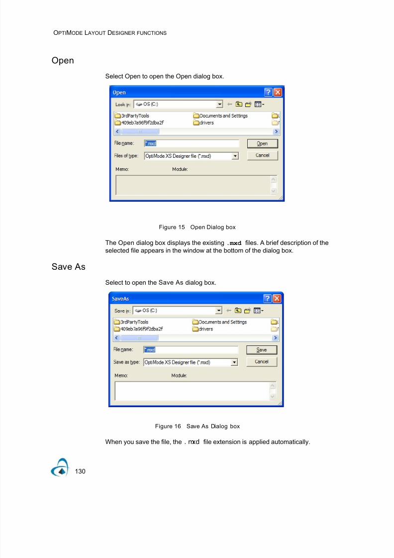
7/21/2019 OptiMode User Reference
http://slidepdf.com/reader/full/optimode-user-reference 134/339
OPTIMODE L AYOUT DESIGNER FUNCTIONS
130
Open
Select Open to open the Open dialog box.
Figure 15 Open Dialog box
The Open dialog box displays the existing .mxd files. A brief description of theselected file appears in the window at the bottom of the dialog box.
Save As
Select to open the Save As dialog box.
Figure 16 Save As Dialog box
When you save the file, the . mxd file extension is applied automatically.

7/21/2019 OptiMode User Reference
http://slidepdf.com/reader/full/optimode-user-reference 135/339
OPTIMODE L AYOUT DESIGNER FUNCTIONS
131
Wafer Properties
Wafer Properties dialog box
Select Wafer Properties to change the wafer properties.
Figure 17 Wafer Properties dialog box - Wafer Dimensions tab
For a description of the fields see the .3D Wafer Properties tab. section on page 28.
Default Waveguide
Select Default Waveguide to change the default waveguide cross section width andprofile.
Figure 18 Default Waveguide Dialog box

7/21/2019 OptiMode User Reference
http://slidepdf.com/reader/full/optimode-user-reference 136/339
OPTIMODE L AYOUT DESIGNER FUNCTIONS
132
Waveguide Default Width: The default width of a waveguide added to the project.
Waveguide Default Profi le: The Profile (defined in the Profile Designer) used bydefault for waveguides added to the project.
Profile Designer:Opens the “Profile Designer” to define and edit Profiles andMaterials.
Profiles and Materials
To open the Profile Designer and create a new material, click Profile Designer . Formore information, “Profile Designer” on page 181
Toolbars
Select the toolbars that you want to make available for the project that you are workingon.
Output Window
The Output Window displays notifications and error messages.
3D Graph Items
To view the following items in the layout, from the View menu, select 3D Graph Items,and then select the item that you want to view. A check mark appears beside theselected item.
Note: The 3D Graph Items are only available in the Ref. Index 2D XZ Plane
View window.
Figure 19 Graph Items - selected items

7/21/2019 OptiMode User Reference
http://slidepdf.com/reader/full/optimode-user-reference 137/339
OPTIMODE L AYOUT DESIGNER FUNCTIONS
133
Palette: Displays the color palette beside the graph.
Figure 20 Palette
For more information on the palette, see .Palette Settings. on page 43.
Ax is : Displays the X-Axis and Y-Axis around the graph.
Height Plot: Displays the height plot view of the graph.
Figure 21 Height Plot view
Image Map: Displays the image map view of the graph.

7/21/2019 OptiMode User Reference
http://slidepdf.com/reader/full/optimode-user-reference 138/339
OPTIMODE L AYOUT DESIGNER FUNCTIONS
134
Figure 22 Image Map view
Plane View (XZ): Displays the plane view along the X and Z axes.
Figure 23 Plane View (XZ)

7/21/2019 OptiMode User Reference
http://slidepdf.com/reader/full/optimode-user-reference 139/339
OPTIMODE L AYOUT DESIGNER FUNCTIONS
135
Plane View (YZ): Displays the plane view along the X and Y axes.
Edit Parameters: Select Edit Parameters to open the Variables and Functions
dialog box.
Figure 24 Variables and Functions dialog box
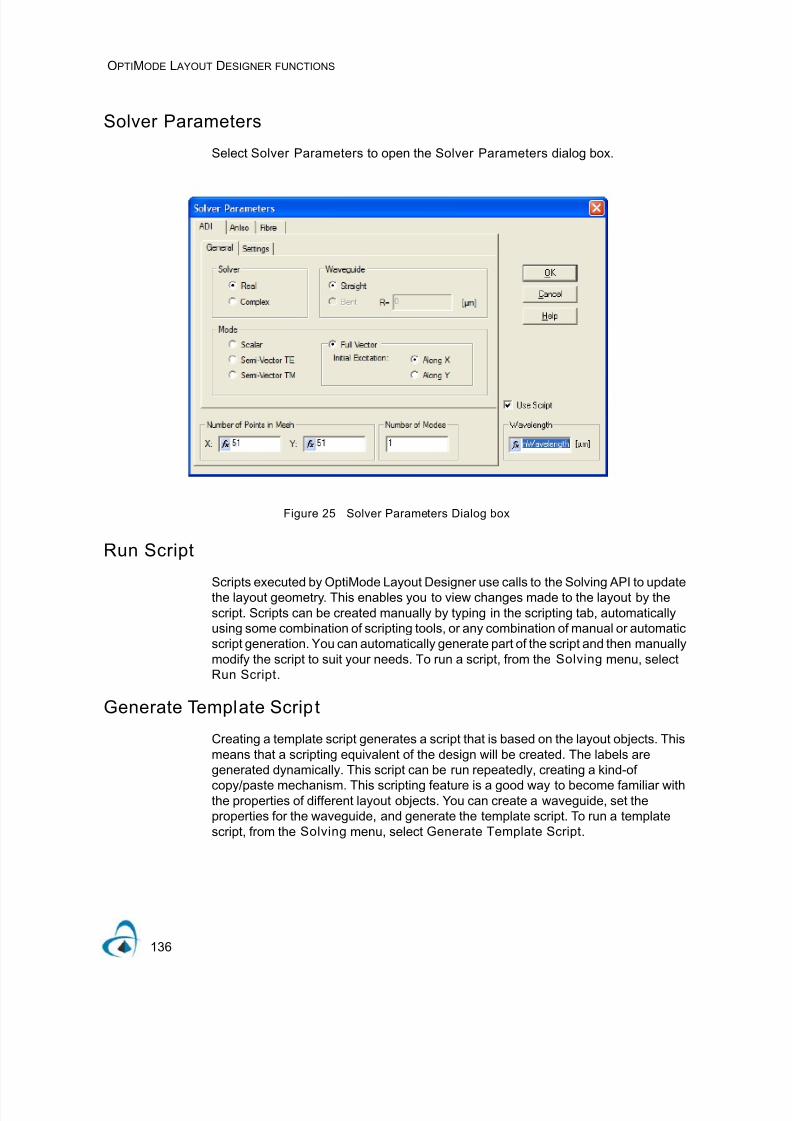
7/21/2019 OptiMode User Reference
http://slidepdf.com/reader/full/optimode-user-reference 140/339
OPTIMODE L AYOUT DESIGNER FUNCTIONS
136
Solver Parameters
Select Solver Parameters to open the Solver Parameters dialog box.
Figure 25 Solver Parameters Dialog box
Run Script
Scripts executed by OptiMode Layout Designer use calls to the Solving API to updatethe layout geometry. This enables you to view changes made to the layout by thescript. Scripts can be created manually by typing in the scripting tab, automaticallyusing some combination of scripting tools, or any combination of manual or automaticscript generation. You can automatically generate part of the script and then manuallymodify the script to suit your needs. To run a script, from the Solving menu, selectRun Script.
Generate Template Script
Creating a template script generates a script that is based on the layout objects. Thismeans that a scripting equivalent of the design will be created. The labels aregenerated dynamically. This script can be run repeatedly, creating a kind-of
copy/paste mechanism. This scripting feature is a good way to become familiar withthe properties of different layout objects. You can create a waveguide, set theproperties for the waveguide, and generate the template script. To run a templatescript, from the Solving menu, select Generate Template Script.

7/21/2019 OptiMode User Reference
http://slidepdf.com/reader/full/optimode-user-reference 141/339
OPTIMODE L AYOUT DESIGNER FUNCTIONS
137
Generate layout script
Creates a layout script that is an exact representation of the layout design. Like thetemplate scripts, the layout script generates script equivalents for waveguides, andinput planes. However, the IDs for the objects will be the same as the IDs in the layout.
Generate scanning script
A scanning script is used primarily as a mechanism to scan parameters. You can scanparameters and manipulate waveguides together in a single script. For example, youcan create a layout with all waveguides having a width set to a .ParamWidth.parameter. When the scanning script runs, the .ParamWidth. value will update asrequired, thus changing all waveguide widths at the same time.
Dispersion scripting
To create a Dispersion script (using an existing layout with at least one waveguide),
click the .Generate Dispersion Script. option in the Solving menu. The DispersionScan dialog box appears.
Figure 26 Dispersion Scan Dialog box
Initial: Wavelength used for the first simulation, a real value in microns.
Final: Wavelength used for the last simulation, a real value in microns. This value hasto be greater than the value in Initial.
Steps: The number of wavelengths to be used. The script will linearly divide the rangedefined by Initial and Final wavelengths to compute the wavelength used at any
given step. The default value is 3. The value cannot be less than three because firstand second order derivatives will be calculated. Note: When using dispersionscripting, Solver Parameters are updated.
To open the Solver Parameters dialog box and define the solver parameters, fromthe Solving menu, select Solver Parameters. In Wavelength, the variable.ScanWavelength” appears which follows the interval defined by Initial and Final
wavelengths. The .Use Script. option is automatically selected.
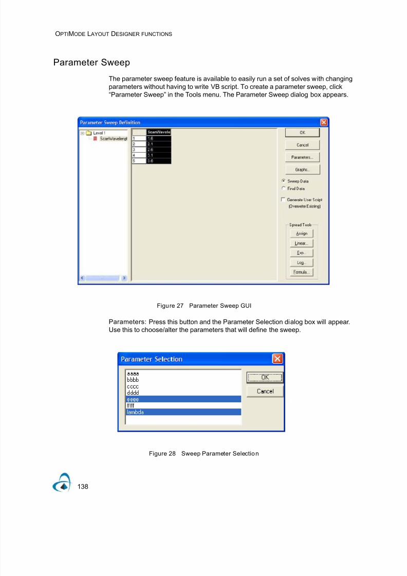
7/21/2019 OptiMode User Reference
http://slidepdf.com/reader/full/optimode-user-reference 142/339
OPTIMODE L AYOUT DESIGNER FUNCTIONS
138
Parameter Sweep
The parameter sweep feature is available to easily run a set of solves with changingparameters without having to write VB script. To create a parameter sweep, click“Parameter Sweep” in the Tools menu. The Parameter Sweep dialog box appears.
Figure 27 Parameter Sweep GUI
Parameters: Press this button and the Parameter Selection dialog box will appear.Use this to choose/alter the parameters that will define the sweep.
Figure 28 Sweep Parameter Selection

7/21/2019 OptiMode User Reference
http://slidepdf.com/reader/full/optimode-user-reference 143/339
OPTIMODE L AYOUT DESIGNER FUNCTIONS
139
Graphs: To define 2D results graphs in the output, choose the Graphs button. The“User Defined Graphs” dialog will appear.
Figure 29 2D Graph Summary
To remove a graph, choose the graph in the “User Defined Graphs” list and click“Remove”.
To Add or Edit a graph, click the appropriate button and teh following dialog willappear.

7/21/2019 OptiMode User Reference
http://slidepdf.com/reader/full/optimode-user-reference 144/339
OPTIMODE L AYOUT DESIGNER FUNCTIONS
140
Figure 30 2D Graph Definition
In the Add/Edit graph dialog, the graph title and X/Y axis names can be entered. Thelist boxes present what values can be put on the axis and how data sets will begrouped in the legend. Defined graphs will be shown at the bottom of the browser tree
by name in the Analyzer.
Figure 31 2D Results Graph Selection
Sweep Data vs Final Data
The Sweep/Final radio buttons toggle between views of the data ranges and the finaldata used for a given iteration step.

7/21/2019 OptiMode User Reference
http://slidepdf.com/reader/full/optimode-user-reference 145/339
OPTIMODE L AYOUT DESIGNER FUNCTIONS
141
Figure 32 Sweep Range Data
Figure 33 Sweep Final Values
In the above examples, lambda has a sweep range of .15 to .55. But when the solverruns, the value at iteration one will be 8, at two, 7, etc. Ranges can be defined forparameters but the final values used in the sweep can be overrideen separately. Innormal use, setting a range will set the final values to be the same by default and no
further changes need to be made.
Spread Tools
The various buttons in this frame can be used to generate ranges in the parametercolumns according to function. First select a column in the parameter grid, thenchoose a function:

7/21/2019 OptiMode User Reference
http://slidepdf.com/reader/full/optimode-user-reference 146/339
OPTIMODE L AYOUT DESIGNER FUNCTIONS
142
Assign: Assigns a single value to all rows of the parameter
Figure 34 Assign Spread Tool
Linear/Exp/Log: Assigns a Linear/Exp/Log range of values to the rows of theparameter.
Figure 35 Range Spread Tool
Formula: Takes a user-defined function and computes a range of values to the rowsof the parameter.

7/21/2019 OptiMode User Reference
http://slidepdf.com/reader/full/optimode-user-reference 147/339
OPTIMODE L AYOUT DESIGNER FUNCTIONS
143
Figure 36 User Function Spread Tool
Level Functions
Figure 37 Sweep Folder Node Options
Right-click on the folder icon of the display tree to:
• Set the number of iterations to sweep over
• Add/Remove levels to sweep
• Add more parameters

7/21/2019 OptiMode User Reference
http://slidepdf.com/reader/full/optimode-user-reference 148/339
OPTIMODE L AYOUT DESIGNER FUNCTIONS
144
Parameter Functions
Figure 38 Sweep Parameter Node Options
Right-click on a parameter in the display tree to:
• Remove a aparameter from the sweep
Move a parameter between levels by left-clicking on it and drag/drop it into anotherfolder.
This effectively sets the variance dependencies.
Figure 39 Sweep Parameter Movement Options
Run Optimization
To run an optimization of selected parameters in the project, select “run Optimization”from the Tools menu.

7/21/2019 OptiMode User Reference
http://slidepdf.com/reader/full/optimode-user-reference 149/339
OPTIMODE L AYOUT DESIGNER FUNCTIONS
145
Figure 40 Optimization Settings
Pick the parameters to optimize from the list on the left. Use the Add/Add All/Remove/Remove All buttons to move parameters in and out of the selected rightside list. Before choosing “Optimize”, the following options can be set:
• The deviance for each parameter
• The Merit function and tolerance
• The type of solve to use (Complex ADI, Real ADI, Aniso, FiberVector,FiberLP)
• The type of optimizer to use (Golden Search, Modified Powell, Nelder-Mead Simplex)
Optimization Results
To view optimization results, choose “Optimization Results” from the tools menu.
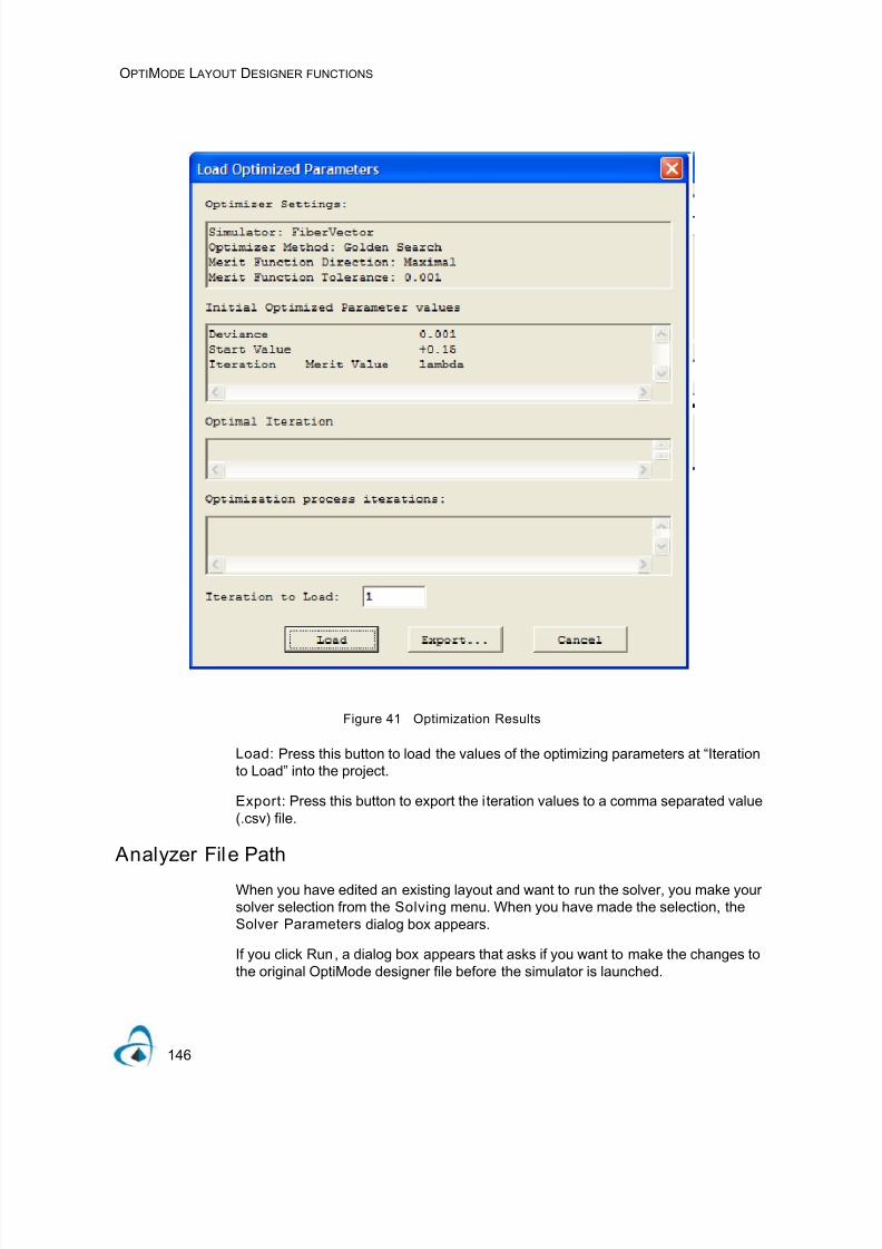
7/21/2019 OptiMode User Reference
http://slidepdf.com/reader/full/optimode-user-reference 150/339
OPTIMODE L AYOUT DESIGNER FUNCTIONS
146
Figure 41 Optimization Results
Load: Press this button to load the values of the optimizing parameters at “Iterationto Load” into the project.
Export: Press this button to export the iteration values to a comma separated value(.csv) file.
Analyzer File Path
When you have edited an existing layout and want to run the solver, you make yoursolver selection from the Solving menu. When you have made the selection, theSolver Parameters dialog box appears.
If you click Run , a dialog box appears that asks if you want to make the changes tothe original OptiMode designer file before the simulator is launched.

7/21/2019 OptiMode User Reference
http://slidepdf.com/reader/full/optimode-user-reference 151/339
OPTIMODE L AYOUT DESIGNER FUNCTIONS
147
Figure 42 OptiMode Designer File Change Dialog box
If you click “Yes”, the original layout design file is changed to reflect the modificationsyou made to the design, and then the simulator is launched. If you click “No”, the Analyzer Fi le Path dialog box appears, asking for the file path/name for thetemporary simulation results file to be created. Click the Browse button to change the
default location. The results saved in this temporary file are used by the OptiMode Analyzer when the simulation is complete.
Figure 43 Analyzer File Path Dialog box

7/21/2019 OptiMode User Reference
http://slidepdf.com/reader/full/optimode-user-reference 152/339
OPTIMODE L AYOUT DESIGNER FUNCTIONS
148
3D Graph Settings
You must click the Ref. Index (n) – 3D XY Plane View tab before you can select itemsfrom the 3D Graph Settings submenu.
Figure 44 Graph Settings Menu and Submenu
Region of Interest
To change the start and end positions of the X and Y axes, from the .Preferences.
menu, select .3D Graph settings > Region o f Interest.. The Region of Interest
dialog box appears.
Note: The start and end values must be integers between 0 and 500.
Figure 45 Region of Interest Dialog box

7/21/2019 OptiMode User Reference
http://slidepdf.com/reader/full/optimode-user-reference 153/339
OPTIMODE L AYOUT DESIGNER FUNCTIONS
149
Height Plot Settings
To change the appearance of the graph, from the .Preferences. menu, select .3D
Graph settings > Height Plot Settings.. The Height Plot Settings dialog boxappears.
Note: Height Plot Settings is only available when the graph is in 3D view.
Figure 46 Height Plot Settings Dialog box
Style: Under Style, you can select from five different styles for the graph.
Rendering: Under Rendering, you can select the type of color interpolation.
Highlighting: The surface area has a more realistic image. However, the highlightscan make it difficult to determine the true color value of the region in the graph.
Depth cue: Fades out less prominent parts of the graph, providing an enhancedperception of the graph.
Hidden Line: This retrieves the line segments that are behind part of the graph. Thiswill not take effect unless the graph style is Wireframe or Lines.
Show Grid: This displays grid lines in the graph.
Grid Density slider: Move the slider to adjust the spacing of the grid lines.
• Low—grid lines are spaced far apart
• High—grid lines are spaced close together

7/21/2019 OptiMode User Reference
http://slidepdf.com/reader/full/optimode-user-reference 154/339
OPTIMODE L AYOUT DESIGNER FUNCTIONS
150
Axis Settings
To change the appearance of the axes, from the “Preferences” menu, select “3D
Graph settings > Axis Settings”. The Axis Settings dialog box appears.
Figure 47 Axis Settings Dialog box
Show Axis: This displays the graph axes.
Font Auto Detail: This changes the font size automatically according to the size ofthe graph window.
Use Axis Scales: Determines how the array data values are scaled. These can bescaled either to the graph‘s X and Y coordinate axes or to the graph‘s z coordinateaxis.
Ax is Style: There are 21 styles available from the drop-down menu. These stylesdetermine how many faces of the view volume are to be displayed.
X-Axis: This setting will include the label, major ticks and minor ticks.
Y-Axis: This setting will include the label, major ticks and minor ticks.
Z-Axis: This setting will include the label, major ticks and minor ticks.
Image Map Settings
To change the appearance of the graph, from the .Preferences. menu, select .3D
Graph settings > Image Map Settings.. The Image Map Settings dialog boxappears.
Note: Image Map Settings is only available when the graph is in the image mapview.

7/21/2019 OptiMode User Reference
http://slidepdf.com/reader/full/optimode-user-reference 155/339
OPTIMODE L AYOUT DESIGNER FUNCTIONS
151
Figure 48 Image Map Settings Dialog box
Image orientation: Under Image orientation, you can adjust the position of the Yand X axes.
Y: Move the Y axis to the left or to the right of the graph.
X: Move the X axis to the top or to the bottom of the graph.
Aspect ratio: Under Aspect ratio, you can select to view the graph in Real
dimensions (one-to-one ratio) or Window dimensions (fits to screen). The ratio ofwidth to height is maintained by the number of points in the array (Y or X) when thegraph window is resized.
Grid Density slider: Move the slider to adjust the spacing of the grid lines.
• Low—grid lines are spaced far apart
• High—grid lines are spaced close together
Linear Filter: Select Linear Filter to blend the adjacent colors of the Image Mapgraphs. If you do not select Linear Filter , the graph will have a tiled appearance.
Show Grid: Displays the grid lines are displayed along the graph.

7/21/2019 OptiMode User Reference
http://slidepdf.com/reader/full/optimode-user-reference 156/339
OPTIMODE L AYOUT DESIGNER FUNCTIONS
152
Palette Settings
To select the color palette or to change how data values for the graph map to colorsin the palette, from the Preferences menu, select 3D Graph settings > Palette
Settings. The Palette Settings dialog box appears.
Figure 49 Palette Settings Dialog box
Use Palette: The current color palette is enabled for graphing.
Auto Ad just : Determines how the data values for a graph are mapped to colors. Ifyou select this option, the minimum data value in the region of interest maps to thebottom of the palette color range, and the maximum data value maps to the top of thepalette color range. All other values map to the color palette proportionally.
Show Palette: Displays the color palette to the right of the graph.
Show Labels: Displays the labels to the right of the color palette. It has no effect ifthe color palette is not shown.
Palette Id: Changes the palette which is used to map data values to colors.
Palette Range: Determines how the data values for a graph map to the current colorpalette. If you do not select Auto Adjust , the palette range has no effect.
Data Clamping Settings
To change the refractive index and the sampling resolution for the graph, from the“Preferences” menu, select “3D Graph settings > Data Clamping Settings”. The
Data Clamping dialog box appears.
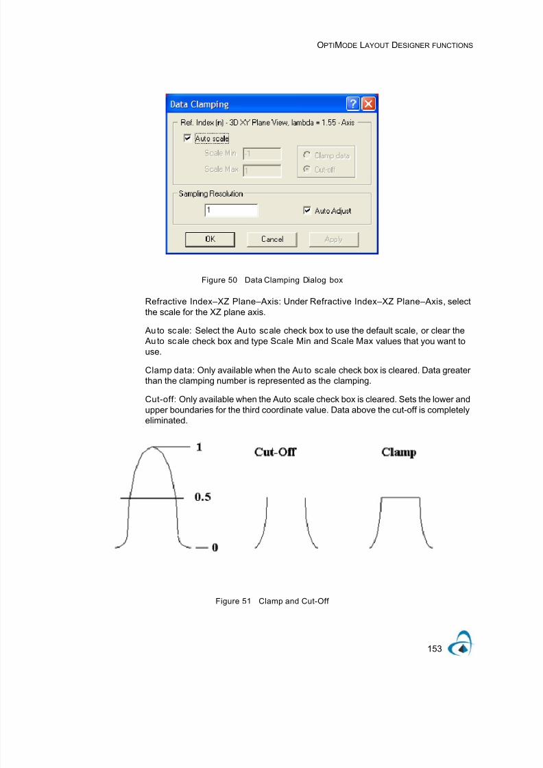
7/21/2019 OptiMode User Reference
http://slidepdf.com/reader/full/optimode-user-reference 157/339
OPTIMODE L AYOUT DESIGNER FUNCTIONS
153
Figure 50 Data Clamping Dialog box
Refractive Index–XZ Plane–Axis: Under Refractive Index–XZ Plane–Axis, selectthe scale for the XZ plane axis.
Au to scale: Select the Auto scale check box to use the default scale, or clear the Au to scale check box and type Scale Min and Scale Max values that you want touse.
Clamp data: Only available when the Auto scale check box is cleared. Data greaterthan the clamping number is represented as the clamping.
Cut-off: Only available when the Auto scale check box is cleared. Sets the lower andupper boundaries for the third coordinate value. Data above the cut-off is completelyeliminated.
Figure 51 Clamp and Cut-Off

7/21/2019 OptiMode User Reference
http://slidepdf.com/reader/full/optimode-user-reference 158/339
OPTIMODE L AYOUT DESIGNER FUNCTIONS
154
Sampling Resolution: If the resolution is set to 1, there is a one-to-one mapping ofdata points to the points in the graph. If the resolution is set to 2, only one out of fourdata points is displayed. Higher incrementing of the resolution value decreases thedetail level of the graph. For example, a resolution of 3 would draw one out of 16points.
Note: Using a lower resolution value (for example 1) enables a more accuratedepiction of the data values in the graph, but can result in slow rendering whendata sets are large.
Auto Ad just : Determines whether the level of detail for graphing will be handledautomatically or with a resolution number. If you select the Auto Adjust check box,the resolution of the graph is adjusted dynamically so that the performance matchesthe demands set by any user activity.
Refract ive Index View
Under Refractive Index View, you can:
• view a 2D (XZ plane) slice of the graph
• view a 3D (XY plane) slice of a graph
Figure 52 RIDX View

7/21/2019 OptiMode User Reference
http://slidepdf.com/reader/full/optimode-user-reference 159/339
OPTIMODE L AYOUT DESIGNER FUNCTIONS
155
Data Visualizer for 64-bit Applications
The 64-bit versions of Layout Designer, Simulators, and Analyzer feature a newredesigned data visualizer (e.g., for the display of the refractive index, etc.). Theinteraction with the visualizer differs from the previous 32-bit version visualizer and is
summarized below.
All interactions with the visualizer are performed using the mouse and keyboardshortcuts. The specifics differ depending on the Height Plot (Surface) or Image Mapview type. The color palette is enabled by default and is situated at the right side ofthe view. The palette and axes can be toggled using the provided GUI functionality.
Zooming in and out - All views
Zooming in and out can be performed using the middle mouse scroll wheel.
Pan, move - All views
Pressing the Right-Mouse-Button and moving the mouse can be used to pan aroundthe view area.
Rotation - Height Plot (Surface) view only
Pressing the Left-Mouse-Button and moving the mouse can be used to rotate thecamera view.
Pan - Height Plot (Surface) view only
Pressing the SHIFT-key + Left-Mouse-Button can be used to pan the view area
Rotation-spin - Height Plot (Surface) view only
Pressing the CTRL-key + Left-Mouse-Button can be used to spin the camera
Zoom in and out - Height Plot (Surface) view only
Pressing the SHIFT-key + CTRL-key + Left-Mouse-Button can be used to zoom thecamera.
The current orientation of the view is shown by the three X-Y-Z axes displayed in thelower left corner of the window. These axes are aligned with the dimensions and axesof the displayed objects.
Switching between the view types will reset the plot (camera) to its default state.
Point Selection
The user has the ability to select a grid point of the displayed objects in Height Plot(Surface) and Image Map views. A click with the Left-Mouse-Button anywhere withinthe object will select the closest data grid point. Information about the data point isprovided in the status text displayed at the bottom of the window.

7/21/2019 OptiMode User Reference
http://slidepdf.com/reader/full/optimode-user-reference 160/339
OPTIMODE L AYOUT DESIGNER FUNCTIONS
156

7/21/2019 OptiMode User Reference
http://slidepdf.com/reader/full/optimode-user-reference 161/339
L AYOUT OBJECTS
157
Layout Objects
There are basically three types of objects available for use in the OptiMode designer:• A cross section waveguide
• A substrate layer definition
• A refractive index file definition
You can place any number of any cross section waveguides in the layout. You canresize and move waveguides anywhere in the wafer by changing their properties.Only one refractive index file definition can be used.
Waveguide vs. wafer
Waveguide width and wafer width
Waveguide width and wafer width are independent—the waveguide can control itswidth. The wafer width is scaled to match the waveguide width at every point alongthe waveguide. All elements in a wafer are scaled by the same factor.
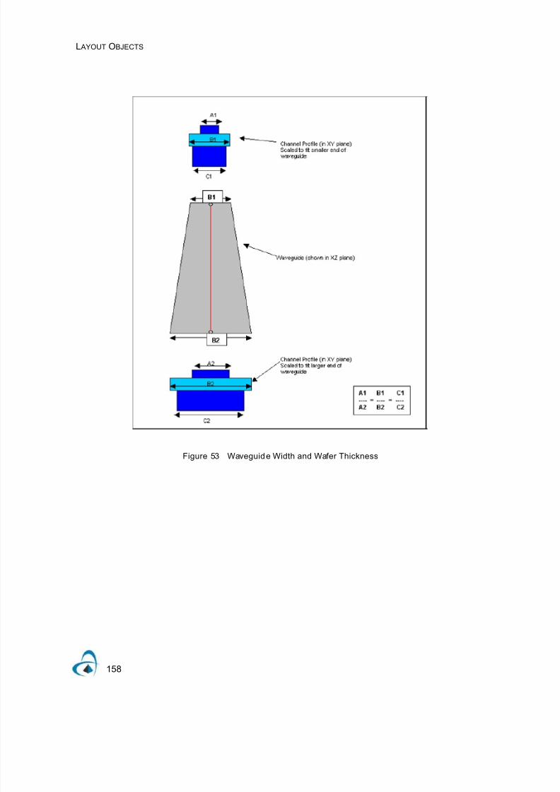
7/21/2019 OptiMode User Reference
http://slidepdf.com/reader/full/optimode-user-reference 162/339
L AYOUT OBJECTS
158
Figure 53 Waveguide Width and Wafer Thickness

7/21/2019 OptiMode User Reference
http://slidepdf.com/reader/full/optimode-user-reference 163/339
L AYOUT OBJECTS
159
Depth description
In OptiMode, the coordinate system is different from the OptiBPM layout view.OptiMode deals with a cross section of the wafer and therefore Y is the OptiBPMdepth and X is profile centering (OptiBPM Y).
Figure 54 Coordinate System
The fiber profile origin is at the center point of the profile. The channel profile origin isat the bottom of the profile. The diffuse profiles are always fixed at a depth = 0.0, andextend down into the substrate.
Figure 55 Depth / Y- value

7/21/2019 OptiMode User Reference
http://slidepdf.com/reader/full/optimode-user-reference 164/339
L AYOUT OBJECTS
160
Depth = 0 at the substrate-cladding interface
Depth < 0 in the substrate
Depth > 0 in the cladding
Depth = cladding thickness at the top of the wafer
Depth = -1 * substrate thickness at the bottom of the wafer
Initial data
The program needs initial data for display and solving. You can change these valuesat any time. Data entry boxes that are marked by the f x symbol can contain anexpression. When you enter a symbolic parameter name instead of numeric data, theprogram looks for known names. If the parameter is not recognized, the programconsiders it a new parameter and prompts for its value. The cladding is a box that youdesign devices in. The width is along the discretization mesh in the X-direction. Theheight is along the discretization mesh in the Y-direction. All refractive indices can becomplex numbers.
User Interface of a Parameterized posi tion of a Layout Shape
Position of most of the shapes placed on the Layout, like cross section waveguides,can be parameterized with user-defined parameters. In such cases, a coordinate(horizontal or vertical) of the layout object position is calculated from the Expressionand Offset values:
Position = Expression + Offset
Parameterization is a very useful feature. Take for example when it is required toadjust the position of a group of waveguides all at the same time. When a group ofwaveguide positions are parameterized with respect to a specific parameter, you caneasily reposition all the waveguides in the group to a desired location by changing the
value of the parameter.
Figure 56 Typical user interface of parameterized Horizontal coordinates
Expression: Accepts arithmetical expressions. You can use standard mathematicalfunctions like sin(), cos(), sqrt(), etc. as well as your own parameters and functionsdefined in the .Edit Parameters. dialog box found under the menu .Simulation ->
Edit parameters..
Offset: Accepts numerical values. The Offset value is added to the value of theExpression, which combined produce the final value of the waveguide Position.Therefore if the position of the waveguide is parameterized (in the Expression), youcan still move the waveguide in the layout designer to adjust the position manually,without affecting the Expression.
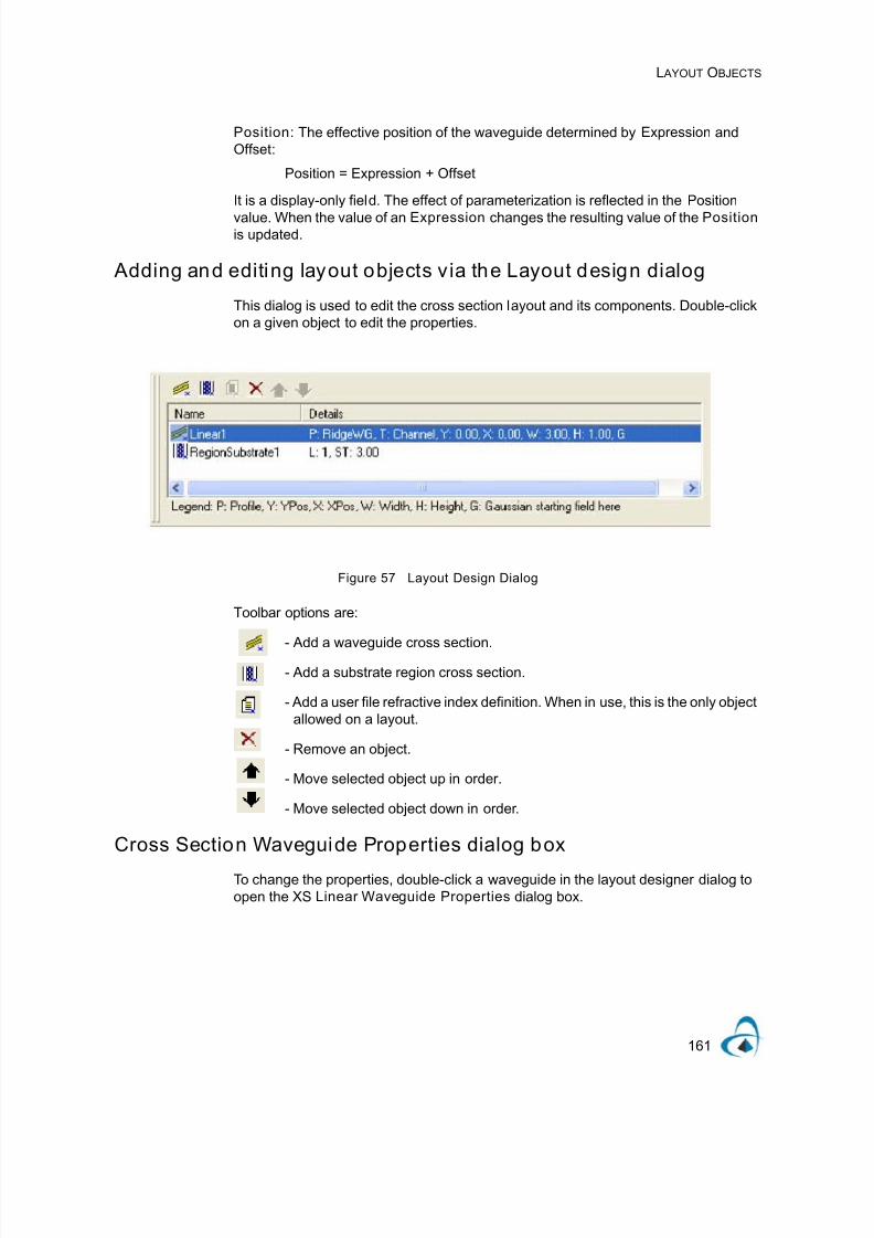
7/21/2019 OptiMode User Reference
http://slidepdf.com/reader/full/optimode-user-reference 165/339
L AYOUT OBJECTS
161
Position: The effective position of the waveguide determined by Expression andOffset:
Position = Expression + Offset
It is a display-only field. The effect of parameterization is reflected in the Position
value. When the value of an Expression changes the resulting value of the Positionis updated.
Adding and editing layout objects v ia the Layout design dialog
This dialog is used to edit the cross section layout and its components. Double-clickon a given object to edit the properties.
Figure 57 Layout Design Dialog
Toolbar options are:
- Add a waveguide cross section.
- Add a substrate region cross section.
- Add a user file refractive index definition. When in use, this is the only objectallowed on a layout.
- Remove an object.
- Move selected object up in order.
- Move selected object down in order.
Cross Section Waveguide Properties dialog box
To change the properties, double-click a waveguide in the layout designer dialog toopen the XS Linear Waveguide Properties dialog box.

7/21/2019 OptiMode User Reference
http://slidepdf.com/reader/full/optimode-user-reference 166/339
L AYOUT OBJECTS
162
Figure 58 Linear Waveguide Properties Dialog box
X Position: Type the center for the waveguide. The center is the position of thewaveguide in the X-direction with respect to the width of the wafer.
Expression: can contain parameters defined using the Edit Parameters dialog boxfound under the Simulation menu > Edit parameters.
Offset: enter value to use with Expression that sets the exact position of thewaveguide.
Position: exact horizontal position of waveguide determined by Expression andOffset.
Remember that these coordinates are different from OptiBPM where you would beviewing from the top of the waveguide.
Y Position: Represents the position on the y-axis of the waveguide with respect to
the top of the substrate. It can be scanned as a parameter. This is equivalent to thedepth in OptiBPM.
Width: Type the width for the waveguide. The width is measured in microns. It can bescanned as a parameter.
Height: Displays the thickness of the waveguide.
Label: The label is a default name that you can change. The new label must beunique among all the labels.
Profile: Every waveguide must be assigned a profile. Select a profile from the Profile
dropdown list. To add profiles to this list, click the Profiles In Use button.
Profiles in Use: Click Profiles in Use to open the Profile Designer and createprofiles and materials. For more information on creating profiles and materials,“Profile Designer” on page 181

7/21/2019 OptiMode User Reference
http://slidepdf.com/reader/full/optimode-user-reference 167/339
L AYOUT OBJECTS
163
Regions
There are two regions available in OptiMode Layout Designer:
• Substrate Region
• User File Region
Substrate Region
Substrate Region dialog box
To access the properties of the Substrate Region, double-click a substrate regionobject in the layout designer dialog to open the Substrate Region dialog box.
Figure 59 Substrate Region Dialog box
Name: The name is a default label that you can change. The new label must beunique among all the labels.
OK: Click to save changes to the region.
Cancel: Click to cancel operation.
Help: Click to load Help files.
Substrate tab
Profile and Material in Use: Click Profile and Material in Use to open the Profile
Designer .

7/21/2019 OptiMode User Reference
http://slidepdf.com/reader/full/optimode-user-reference 168/339
L AYOUT OBJECTS
164
Substrate Layers
The Substrate layers window displays the names of the substrate layers and thesettings for each layer.
Figure 60 Substrate Layers window
Delete: Click Delete to delete the layer selected in the Substrate layers window.
Add/Ed it : Click Add or Edit to open the Layers dialog box and add a layer to theSubstrate layers window.
Figure 61 Layers Dialog box
Thickness: Specify the layer thickness.
Material: Specify the layer material.
Material in Use: Click .Material in Use. to open the Profile Designer.
User File Region
User File Region dialog box
To access the properties of the User File Region, double-click the user file region inthe layout designer dialog to open the User File Region dialog box.

7/21/2019 OptiMode User Reference
http://slidepdf.com/reader/full/optimode-user-reference 169/339
L AYOUT OBJECTS
165
Figure 62 User File Region Dialog box
Name: The name is a default label that you can change. The new label must beunique among all the labels.
OK: Click to save changes to the region.
Cancel: Click to cancel operation.
Help: Click to load Help files.
3D User File tab
Wafer Width X: Displays the wafer width in the x-direction as loaded from the datafile.
Wafer Width Y: Displays the wafer width in the y-direction as loaded from the data file.
Nx: The number of mesh points in the x-direction taken from the selected fi le.
Ny: The number of mesh points in the y-direction taken from the selected fi le.
Propagation Type: Displays the type of the refractive index distribution data fileformat. There are two data file format types:
Propagation Dependent: Contains a refractive index distribution slice for everycalculation step. If the file is short of data slices, then the last loaded refractive index
distribution slices fed to the calculation engine for every remaining calculation stepwithin the User File Region.
Propagation Independent: Contains a single refractive index distribution slice. Theslice is loaded from the file and fed to the calculation engine for every calculation stepwithin the User File Region. The refractive index distribution is the same at everycalculation step, so the program does not need to read the refractive index slice aftereach step.
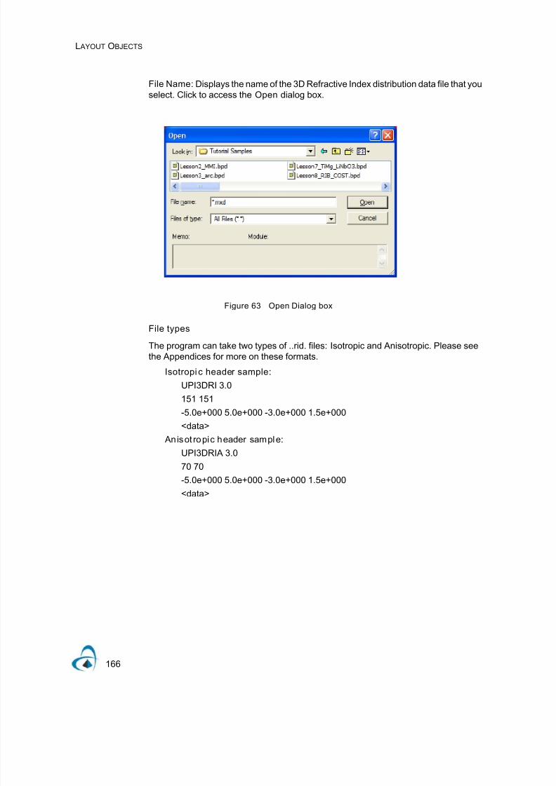
7/21/2019 OptiMode User Reference
http://slidepdf.com/reader/full/optimode-user-reference 170/339
L AYOUT OBJECTS
166
File Name: Displays the name of the 3D Refractive Index distribution data file that youselect. Click to access the Open dialog box.
Figure 63 Open Dialog box
File types
The program can take two types of ..rid. files: Isotropic and Anisotropic. Please seethe Appendices for more on these formats.
Isotropi c header sample:
UPI3DRI 3.0
151 151
-5.0e+000 5.0e+000 -3.0e+000 1.5e+000<data>
An isot ropic header sample:
UPI3DRIA 3.0
70 70
-5.0e+000 5.0e+000 -3.0e+000 1.5e+000
<data>

7/21/2019 OptiMode User Reference
http://slidepdf.com/reader/full/optimode-user-reference 171/339
L AYOUT OBJECTS
167
Solving
After you complete a design project in OptiMode Layout Designer that contains all ofthe required elements, you can run a solver. This section describes the solvingparameters.
Variables and Functions dialog box
The Variables and Functions dialog box is the editing environment where you canadd or modify user variables and user functions. To open the Variables and
Functions dialog box, from the OptiMode Layout Designer Simulation menu, selectEdit Parameters.
Figure 64 Variables and Functions Dialog box
User Variable tab A user variable is helpful for constructing user functions. The user variable has asymbolic name and a numerical value determined by an expression. The expressiondefining the variable can be a mathematical formula containing existing parameters,variables, and functions. For example, type the name Myvar and assign to it theexpression 2*pi/Lambda.
Name: Must be unique across all variables.

7/21/2019 OptiMode User Reference
http://slidepdf.com/reader/full/optimode-user-reference 172/339
L AYOUT OBJECTS
168
Expression: Any single line mathematical equation that can be parsed by theOptiMode parser. For more information, “Appendix C: Parser supported functions” onpage 317
Value: After the Name and Expression are entered, click Verify to display the value
in the edit field.
Verify button : Click to evaluate the expression and display the result in the read onlyedit box.
Add/App ly button: Click to add a new variable or change existing variables.
User Variables tab: The User Variables tab displays the list of all the defined uservariables and their expressions.
Figure 65 User Variables tab
User Functions/DLL‘s tab: A list of user functions that have been defined and DLLfunctions that have been introduced so far, using the user function and user DLLfunction.
Figure 66 User Functions/DLLs tab

7/21/2019 OptiMode User Reference
http://slidepdf.com/reader/full/optimode-user-reference 173/339
L AYOUT OBJECTS
169
User Function tab
A user function has a name and a number of symbolic arguments.
Figure 67 User Function tab
To specify the user function, enter its name followed by the arguments list inparentheses—for example, Myfun(x,y), where x and y are the arguments. Thefunction is defined by an expression that can be a mathematical formula containingthe arguments, existing parameters, user variables, and functions. At the moment offunction definition, the arguments do not have numerical values. The function is notevaluated even if expressed with the help of additional parameters and user variableshaving numerical values well defined. The function definition forms only a template.
The function will be evaluated in numerical simulations only after assigning values tothe function arguments. For example, the function can be defined as:Myvar*Width*exp(-(x*x+y*y)), where =Width‘ is a parameter equal to 4 and =Myvar‘ isa user variable equal to 3. Still, the function value is not determined since the valuesof x and y is not known. You can limit the function by specifying the argument limits,for example enter the expression: x*x+y*y<1 to limit the function domain by a circleof radius 1. This function can also be limited by using the variable_FnRslt_ which isthe function value. For example, enter the Limits expression: abs( _FnRslt_ )<1 toassure that the function is clipped when its absolute value is equal to or exceeds 1.Click Add/Apply, add the function definition to the list of user functions. _FnRslt_
represents a result value of the base function execution for a given set of arguments.(These are predefined for use in the Domain Function expressions.)
Parser Function Declaration
In the function specification box, you provided the function name, dltn, followed by theargument list in parenthesis, (x,y,W). Generally, in the function expression box, youcan use the arguments and other variables. However, you may choose not to usesome of the arguments in your expression. In the present expression, we use all thearguments x, y, and W, as well as the parameters, Dx, Dy, and F, and the uservariables, C0 and d, previously introduced. Notice that the program offers an

7/21/2019 OptiMode User Reference
http://slidepdf.com/reader/full/optimode-user-reference 174/339
L AYOUT OBJECTS
170
extensive list of mathematical functions that are pre-defined. Here, we used the errorfunction, erf(...), and the exponent function, exp(...), from the pre-defined functionlibrary. Notice that only the parameters and user variables have numerical values,while the function arguments x,y and W are not determined yet. Their values will comelater from the layout (see below about the Argument Association dialog box).
Example Select the User Process tab. Assign the user function to the user processas follows:
Function name: upr1(x,y,W)
Expression : dltn(x,y,W)
Process name: UserDef1:LiNbO3
Now, your function is ready to be used in the user process definition. We will assignthe index profile function dltn(x,y,W) to the user process function upr1(x,y,W).
To assign the function expression you can just drag the string 'dltn(x,y,W)' from the
User Functions tab below and drop it in the Expression box of the User Process tab.
Function specification: Specifies the function name and the parameter list.
Expression: Declares a single line function that can be parsed by the parser.
Limits: Define a set of limits on the function parameters or the function result.
Use limi ts check box: Determines whether or not the limits are used.
Verify button: Click to evaluate the expression and displays the result in the read onlyedit box.
Add/App ly button: Click to add a new variable or change the existing variable.
User Variables tab: Displays the list of all the defined user variables and theirexpressions.
User Functions/DLL‘s tab: A list of user functions that have been defined and DLLfunctions that have been introduced so far, using the user function and user DLLfunctions.
DLL Function tab
A DLL file with the extension *. dl l contains computer code describing the processfunction.

7/21/2019 OptiMode User Reference
http://slidepdf.com/reader/full/optimode-user-reference 175/339
L AYOUT OBJECTS
171
Figure 68 DLL Function tab
You can assign a diffusion process function defined in a Dynamic Link Library (DLL). A DLL file contains computer code describing the process function. To apply afunction defined in the DLL you must provide the exact name and number ofarguments of the DLL function. This is done in the Function Specification box. Nextyou must provide the name of the DLL where the specified function is defined. Theprogram assumes that user DLLs are placed in the "\UserDLLs" subdirectory.
Alternatively, you may browse to a DLL to provide the full path. To ensure that yourfunction specification agrees with the selected DLL, press Verify. The arguments ofthe process function must be linked to the layout variables as for other user
processes. To link these variables, press Assign.
Function specification: The function specification has to match the functionprovided by the DLL.
DLL: Name of the DLL that contains function code.
Verify button: Click to evaluate the expression and displays the result in the read onlyedit box.
Add/App ly button: Click to add a new variable or change the existing variable.
User Variables tab: Displays the list of all the defined user variables and theirexpressions.
User Functions/DLL‘s tab: A list of user functions that have been defined and DLLfunctions that have been introduced so far, using the user function and user DLLfunctions.

7/21/2019 OptiMode User Reference
http://slidepdf.com/reader/full/optimode-user-reference 176/339
L AYOUT OBJECTS
172
Solver Parameters
To open the Solver Parameters dialog box, from the Solver menu, select Solver
Parameters.
ADI General TabThis tab displays parameters used in the Alternate Direction Implicit simulationmethod.
Figure 69 ADI Solver Parameters Dialog box – ADI General tab
Solver : ADI solver can be real or complex. The real solver deals will find modes withreal effective index (real propagation constant), and the complex solver can find lossyor leaky modes as well as the real ones.
Real: Use this option when you want to find an ideal lossless guided mode. The modalindex will be a real number.
Complex: Use this option when you expect the mode will have losses. The loss couldresult either from lossy materials in the waveguide or from a leaky waveguide.
Waveguide: The mode solving will be done on a straight waveguide. Mode solvingon bent waveguides is currently unavailable.
Mode
Scalar : The solver works in the simplest scalar mode.
Semi-Vector TE: The solver finds transverse electric modes.

7/21/2019 OptiMode User Reference
http://slidepdf.com/reader/full/optimode-user-reference 177/339
L AYOUT OBJECTS
173
Semi-Vector TM: The solver finds transverse magnetic modes.
Full Vector : For this option, you can select the initial excitation field: along the X or Ydirection.
Initial Excitation along X:If the initial field is parallel to the x axis, you can expect tofind a quasi-TE mode.
Initial Excitation along Y: If the initial field is parallel to the y axis, you can expect tofind a quasi-TM mode this way.
Use Script: If this checkbox is enabled, the simulation will proceed according to VBScript commands found in the Scripting page. Otherwise, the simulation is performedonce according to current settings, ignoring any script written in the Scripting page.
Wavelength: This is the optical wavelength, in microns, to be used in this modesolving. The fx symbol means that the value can be specified as a User Parameterinstead of a number.
Number of poin ts in Mesh: Enter the number of points along X and Y meshdirections.
X: The width of the calculation window will have a mesh with this number of points.
Y: The height of the calculation window will be meshed with the number of points.
Number of Modes: Maximum number of guided modes to be found.

7/21/2019 OptiMode User Reference
http://slidepdf.com/reader/full/optimode-user-reference 178/339
L AYOUT OBJECTS
174
ADI Sett ings tab
Figure 70 ADI Settings tab
Starting Field: The starting field is for initial excitation of the waveguide. By default,the Gaussian option is selected. You can modify the Gaussian field by clickingProperties and entering your data in the Gaussian Starting field dialog box. You canselect a Gaussian field or supply a user-defined field from file.
Gaussian : In the Gaussian Starting Field, you can set up the Gaussian starting fieldfor the BPM simulation. The Gaussian field is defined by:
where x is the transverse layout coordinate, x0 is the center position, and is the fieldhalf-width.
File: Use this option if you want to supply your own starting field from a file.
Properties: Clicking the Properties button will prompt the Gauss Field Parametersdialog box.
E x( ) x x0 –
σ-------------
⎝ ⎠⎛ ⎞
2
– exp=
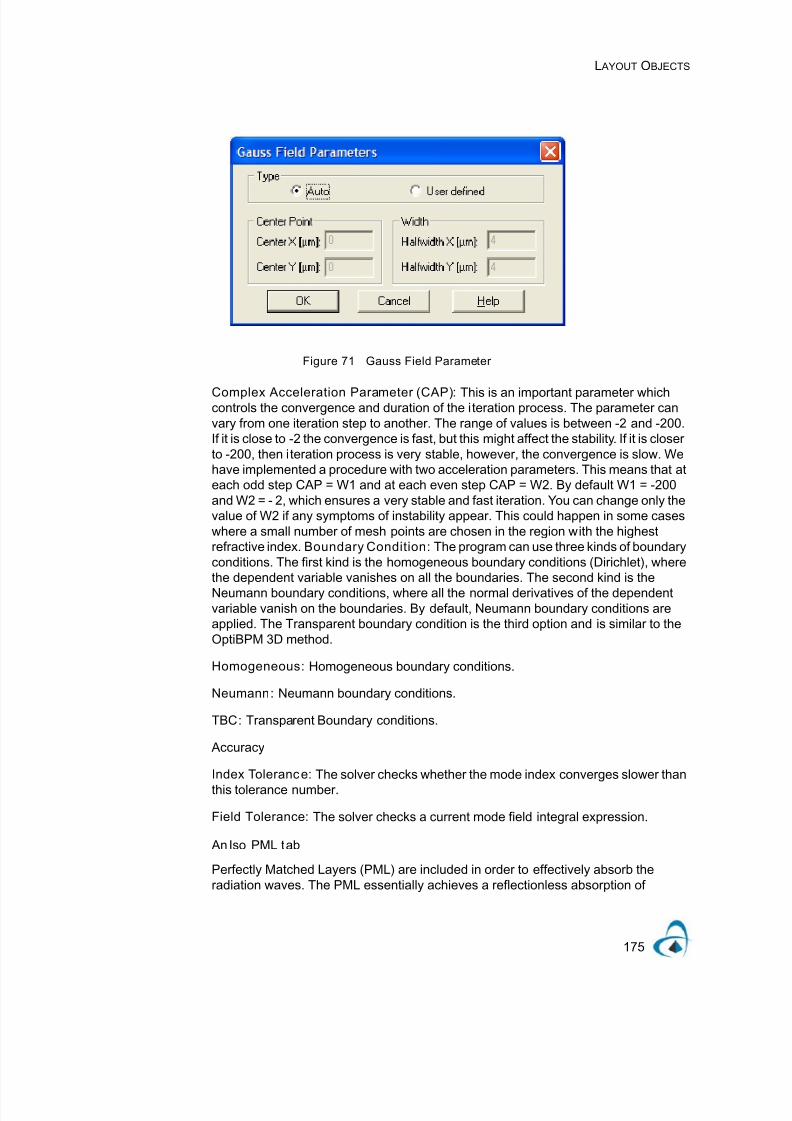
7/21/2019 OptiMode User Reference
http://slidepdf.com/reader/full/optimode-user-reference 179/339
L AYOUT OBJECTS
175
Figure 71 Gauss Field Parameter
Complex Acceleration Parameter (CAP): This is an important parameter whichcontrols the convergence and duration of the iteration process. The parameter canvary from one iteration step to another. The range of values is between -2 and -200.If it is close to -2 the convergence is fast, but this might affect the stability. If it is closerto -200, then iteration process is very stable, however, the convergence is slow. Wehave implemented a procedure with two acceleration parameters. This means that ateach odd step CAP = W1 and at each even step CAP = W2. By default W1 = -200and W2 = - 2, which ensures a very stable and fast iteration. You can change only thevalue of W2 if any symptoms of instability appear. This could happen in some caseswhere a small number of mesh points are chosen in the region with the highestrefractive index. Boundary Condition: The program can use three kinds of boundaryconditions. The first kind is the homogeneous boundary conditions (Dirichlet), wherethe dependent variable vanishes on all the boundaries. The second kind is the
Neumann boundary conditions, where all the normal derivatives of the dependentvariable vanish on the boundaries. By default, Neumann boundary conditions areapplied. The Transparent boundary condition is the third option and is similar to theOptiBPM 3D method.
Homogeneous: Homogeneous boundary conditions.
Neumann: Neumann boundary conditions.
TBC: Transparent Boundary conditions.
Accuracy
Index Tolerance: The solver checks whether the mode index converges slower than
this tolerance number.
Field Tolerance: The solver checks a current mode field integral expression.
An Iso PML tab
Perfectly Matched Layers (PML) are included in order to effectively absorb theradiation waves. The PML essentially achieves a reflectionless absorption of

7/21/2019 OptiMode User Reference
http://slidepdf.com/reader/full/optimode-user-reference 180/339
L AYOUT OBJECTS
176
electromagnetic waves in the continuum limit as the mesh discretization size goes tozero. The absorption inside the PML operates through conductive losses, so that anexponential decay for the field inside the PML is obtained. When a PML regionsurrounds the computational domain, the spurious reflection from the grid boundariescan be made exponentially smaller. It is demonstrated that PML is extremely effective
in absorbing out-going traveling waves of a wide special spectrum.
Figure 72 AnIso PML tab
Number of Layers: Thickness of PML region in mesh points for calculation.
Theoretical Reflection Coefficient: Theoretical reflection coefficient R at theinterface between the computational window and the PML medium.
Power of the Grading Polynomial: The power of the function that defines the PMLparameters (Power of the Grading Polynomial).
Use Script: If this checkbox is enabled, the simulation will proceed according to VBScript commands found in the Scripting page. Otherwise, the simulation is performedonce according to current settings, ignoring any script written in the Scripting page.
Wavelength: This is the optical wavelength, in microns, to be used in this modesolving. The fx symbol means that the value can be specified as a User Parameterinstead of a number.
Number of poin ts in Mesh: Enter the number of points along X and Y meshdirections.
X: The width of the calculation window will have a mesh with this number of points.
Y: The height of the calculation window will be meshed with the number of points.
Number of Modes: Maximum number of guided modes to be found.
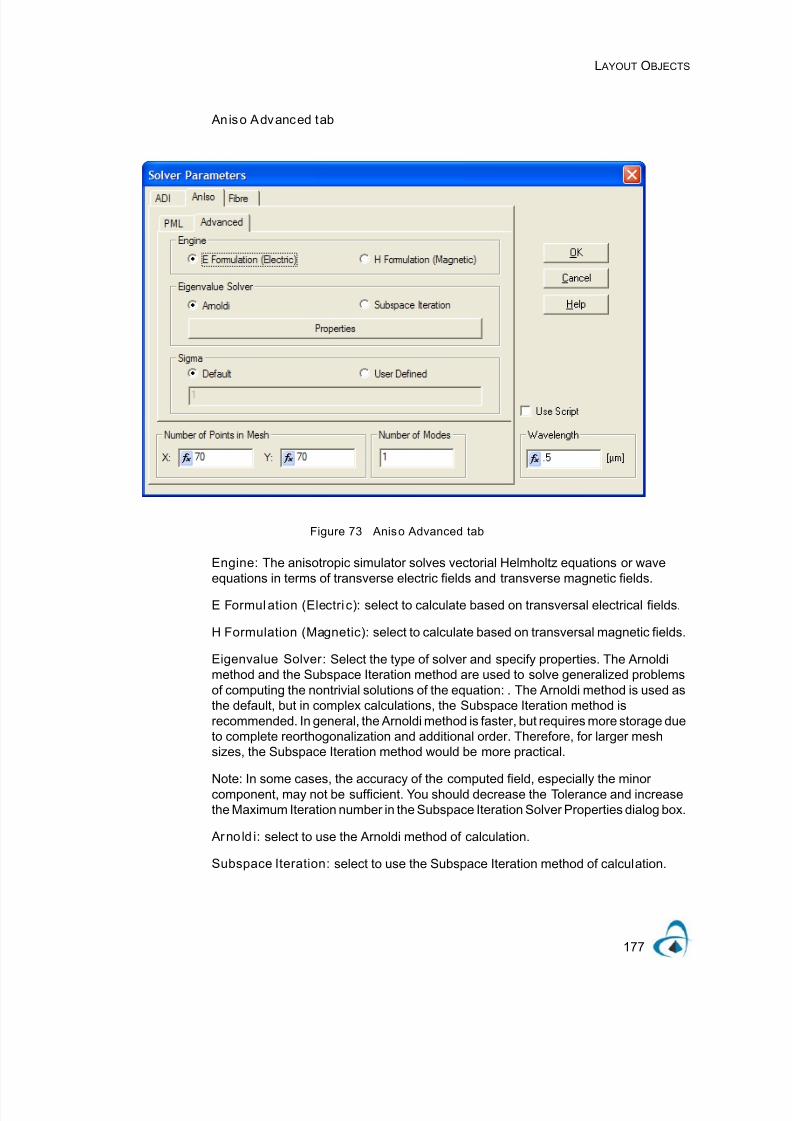
7/21/2019 OptiMode User Reference
http://slidepdf.com/reader/full/optimode-user-reference 181/339
L AYOUT OBJECTS
177
An iso Advanced tab
Figure 73 Aniso Advanced tab
Engine: The anisotropic simulator solves vectorial Helmholtz equations or waveequations in terms of transverse electric fields and transverse magnetic fields.
E Formulation (Electri c): select to calculate based on transversal electrical fields.
H Formulation (Magnetic): select to calculate based on transversal magnetic fields.
Eigenvalue Solver : Select the type of solver and specify properties. The Arnoldimethod and the Subspace Iteration method are used to solve generalized problemsof computing the nontrivial solutions of the equation: . The Arnoldi method is used asthe default, but in complex calculations, the Subspace Iteration method isrecommended. In general, the Arnoldi method is faster, but requires more storage dueto complete reorthogonalization and additional order. Therefore, for larger meshsizes, the Subspace Iteration method would be more practical.
Note: In some cases, the accuracy of the computed field, especially the minorcomponent, may not be sufficient. You should decrease the Tolerance and increasethe Maximum Iteration number in the Subspace Iteration Solver Properties dialog box.
Arno ld i: select to use the Arnoldi method of calculation.
Subspace Iteration: select to use the Subspace Iteration method of calculation.

7/21/2019 OptiMode User Reference
http://slidepdf.com/reader/full/optimode-user-reference 182/339
L AYOUT OBJECTS
178
Properties: click to open the properties dialog box of the selected method (seedialogs for Arnoldi properties and for Subspace Iteration properties).
Sigma: Sigma is the starting value used to find the modal index. For anisotropiccalculations, sigma is the highest element (absolute value) of the permittivity tensor
for the anisotropic structure.
Default: default sigma value for mode solving calculations.
User Defined: user-defined sigma value for mode solving calculations. Select toactivate field to enter value. This value should be as close as possible to the squareof the modal index.
Fiber tab
Figure 74 Fiber tab
Order : All fiber modes have an angular mode number for azimuthal variations calledOrder. This integer is the first integer in the mode name. For example, LP (0, 3) is alinearly polarized mode with no variation of the field in the azimuth.
Order From / To: The Fiber mode solver will find modes of all Orders within thespecified From and To range. The calculation will be done one Order at a time. Allmodes in the current Order are found before the next Order is calculated. If thenumber of modes found is greater than Max. Mode Count, the calculation of thecurrent Order will stop and the algorithm will go on to the calculation of the next Order.

7/21/2019 OptiMode User Reference
http://slidepdf.com/reader/full/optimode-user-reference 183/339
L AYOUT OBJECTS
179
Max. Mode Count: Within each Order, this Max number will limit the number ofmodes found in each Order. Once it has found Max modes in order n, it will stop thecalculation of Order n and go on to the calculation of modes with Order n + 1.
Accuracy, Modal Index Tolerance: This is the level of accuracy in the modal index
of the solution.
Accuracy, Cut-Of f Reject ion Tolerance: In searching for modes, spurious solutionsare sometimes found at the maximum refractive index and the cladding index. Forexample, there might be a spurious mode found whose modal index is equal to thecladding index. To prevent these from appearing in the list of modal solutions, themode solver rejects modes whose modal index differs from the cladding index by lessthan this rejection tolerance.
Rotation: The Fiber, being circular, has no preferred orientation in the transverseplane. The field solutions, on the other hand, usually do show a preferred direction. Itmight be required to orient the field solution in a specific direction. This can beachieved by setting the rotation (in degrees) to rotate the field about the fiber axis as
desired.

7/21/2019 OptiMode User Reference
http://slidepdf.com/reader/full/optimode-user-reference 184/339
L AYOUT OBJECTS
180

7/21/2019 OptiMode User Reference
http://slidepdf.com/reader/full/optimode-user-reference 185/339
PROFILE DESIGNER
181
Profile Designer
Profile Designer When you create a new project in OptiMode Layout Designer, you must define theprofiles and materials for the project in the Profile Designer.
Figure 75 Profile Designer
Main parts of the GUI
The Profile Designer GUI contains three main windows:
• Library Browser
• Layout
• Output

7/21/2019 OptiMode User Reference
http://slidepdf.com/reader/full/optimode-user-reference 186/339
PROFILE DESIGNER
182
Library Browser
Displays a directory where all profile and material data are stored. The Master listcontains profiles and materials for all projects. OptiMode XSDesigner1 list containsprofiles and materials for a specific project.
Figure 76 Library Browser
Layout window
The Layout Window is the main working area where you define the settings for theprofiles and materials.

7/21/2019 OptiMode User Reference
http://slidepdf.com/reader/full/optimode-user-reference 187/339
PROFILE DESIGNER
183
Figure 77 Layout Window
Output window
The Notification and Error tabs display any notifications or errors that occur.
Figure 78 Output Window
Main menu bar
The main menu bar contains the menus that are available in Profile Designer. Manyof these menu items are also available as buttons on the toolbars.
Figure 79 Main Menu bar

7/21/2019 OptiMode User Reference
http://slidepdf.com/reader/full/optimode-user-reference 188/339
PROFILE DESIGNER
184
Toolbars
The Library Browser toolbar is the only toolbar available in Profile Designer.
Figure 80 Profile Designer - Library Browser toolbar
Library Browser toolbar
Library Browser
Library Browser
menu item
Toolbar
button
Description
New Create a new material (the default is dielectric). Select a different material type from
the drop-down list.
Rename Only available when you select a material. Click to rename the selected material.
Delete Only available when you select a material. Click to delete the selected material.

7/21/2019 OptiMode User Reference
http://slidepdf.com/reader/full/optimode-user-reference 189/339
PROFILE DESIGNER
185
Find Click to search for a material. The Find dialog box appears.
Properties Only available when you select a material. Click to view the general properties of the
selected material.
Library Browser
menu item
Toolbar
button
Description

7/21/2019 OptiMode User Reference
http://slidepdf.com/reader/full/optimode-user-reference 190/339
PROFILE DESIGNER
186

7/21/2019 OptiMode User Reference
http://slidepdf.com/reader/full/optimode-user-reference 191/339
PROFILE DESIGNER MENUS
187
Profile Designer menus
This section describes the menus and buttons available in Profile Designer.
File menu
Edit menu
View menu
Tools menu
Fi le menu i tem Descr ipti on
Exit Closes Profile Designer. Any unsaved materials will be lost.
Edit menu item Descr ipti on
Delete Removes all selected materials.
Cut Removes all selected materials and places them on the clipboard.
Copy Copies selected materials and places them on the clipboard. The selected materials remain in the
active file, but they are also placed on the clipboard.
Paste Copies materials from the clipboard and pastes them in a user-defined location.
View menu i tem Descr ip tion
Status Bar Displays the status bar at the bottom of the window.
Library Browser Displays the Library Browser.
Output Window Displays the Output Window.
Tools menu i tem Descript ion
Compare andCopy Libraries
Compare two libraries to see if the listed items are equivalent, conflicted, or unique.
Merge contents of one master.plb file into another.
Edit variable andfunction Edit, add, or modify user variables and user functions.
Mode (Ctrl-M) Opens the Global Data:ADI Method dialog box for selecting mode settings.
Mode Settings Type the setting for the cladding, substrate, wafer, and mesh.

7/21/2019 OptiMode User Reference
http://slidepdf.com/reader/full/optimode-user-reference 192/339
PROFILE DESIGNER MENUS
188
Help menu
Help menu i tem Descr ip tion
Help Topics Provides information on Profile Designer.
About Pro fi leDesigner
Provides information about Optiwave — mailing address, telephone and fax numbers, URL, and e-
mail address.

7/21/2019 OptiMode User Reference
http://slidepdf.com/reader/full/optimode-user-reference 193/339
PROFILE DESIGNER FUNCTIONS
189
Profile Designer functions
This section contains descriptions of the functions and dialog boxes that you accessfrom Profile Designer menus.
Note: Standard Windows functions and dialog boxes are not described.
Library Browser
Materials that you create for a project are stored in the Library Browser under theproject name. There is a separate library for each project, as well as a master library.You can copy materials from one library into another.
Compare Libraries
You can compare two different libraries from any open projects to see if the materialsin the two libraries are equivalent, conflicted, or unique.
To compare two libraries, open the Compare Libraries dialog box (see Figure 81).

7/21/2019 OptiMode User Reference
http://slidepdf.com/reader/full/optimode-user-reference 194/339
PROFILE DESIGNER FUNCTIONS
190
Figure 81 Compare Libraries dialog box
By default, the project selected in the Library Browser appears in the Library 1 window (see Figure 82).
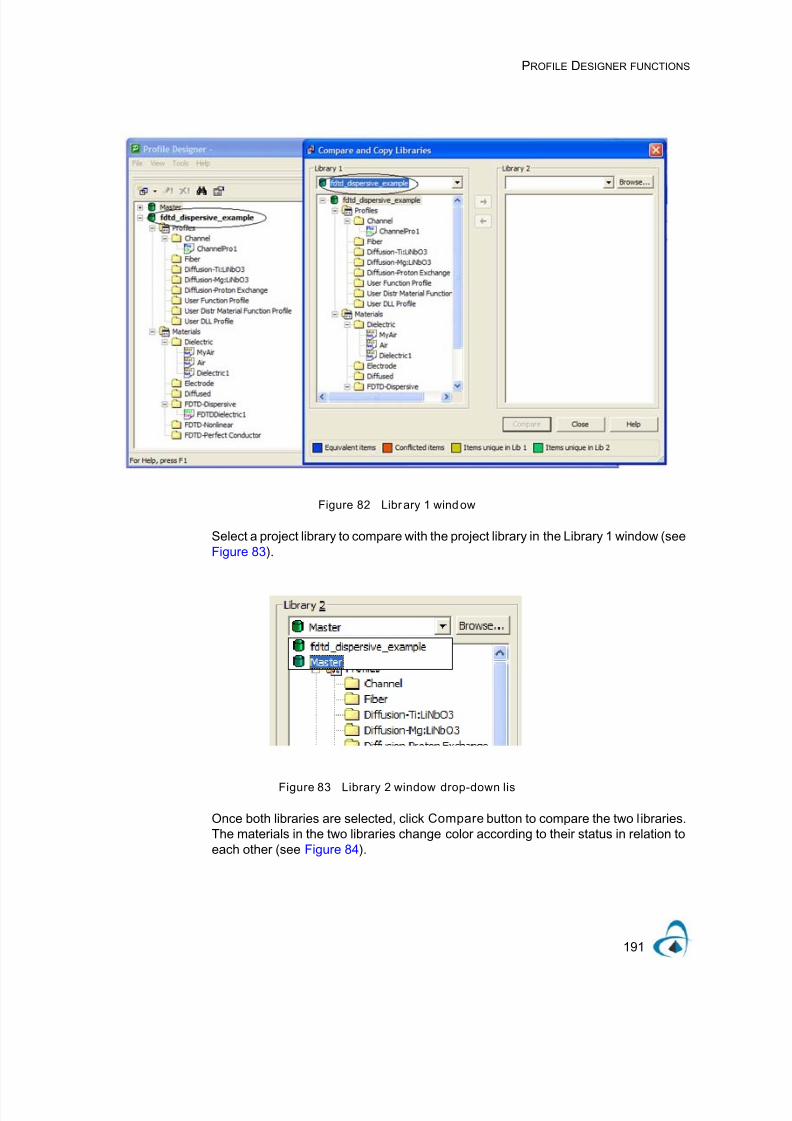
7/21/2019 OptiMode User Reference
http://slidepdf.com/reader/full/optimode-user-reference 195/339
PROFILE DESIGNER FUNCTIONS
191
Figure 82 Library 1 window
Select a project library to compare with the project library in the Library 1 window (seeFigure 83).
Figure 83 Library 2 window drop-down lis
Once both libraries are selected, click Compare button to compare the two libraries.The materials in the two libraries change color according to their status in relation toeach other (see Figure 84).

7/21/2019 OptiMode User Reference
http://slidepdf.com/reader/full/optimode-user-reference 196/339
PROFILE DESIGNER FUNCTIONS
192
Figure 84 Material Names - coloured
Compare the color codes at the bottom of the screen with the color of the materialnames to determine the status of the materials in Library 1 and Library 2.
• Blue —Equivalent items
• Red —Conflicted items
• Yellow —Items unique in Lib 1
• Green —Items unique in Lib 2

7/21/2019 OptiMode User Reference
http://slidepdf.com/reader/full/optimode-user-reference 197/339
PROFILE DESIGNER FUNCTIONS
193
Edit Variables and Functions
Select a project from the Library Browser and open the Variables and Functions dialog box to add or modify user variables and functions.
Note: The name in the title bar indicates whether or not the project has beenopened from the Master List or the regular OptiMode Layout Designer.
Mode Solver(s)
All OptiMode solvers are accessible through the Profile Designer. They use basicwaveguide and wafer definitions provided by the user to solve with.
Figure 85 Mode Solver Options
For information on specific solver settings, please see the section “SolverParameters” on page 136. All solvers also contain the wafer and waveguide propertypages for user input.

7/21/2019 OptiMode User Reference
http://slidepdf.com/reader/full/optimode-user-reference 198/339
PROFILE DESIGNER FUNCTIONS
194
Wafer tab
Figure 86 Global Data: ADI Method—Wafer tab
Cladding: Material name and thickness.
Substrate: Material name and thickness.
Dimensions, Width: Wafer width.
Dimensions, Thickness: Wafer thickness (calculated).

7/21/2019 OptiMode User Reference
http://slidepdf.com/reader/full/optimode-user-reference 199/339
PROFILE DESIGNER FUNCTIONS
195
Waveguide tab
Figure 87 Global Data: ADI Method—Waveguide tab
Depth: Waveguide depth.
Position: Waveguide position.
Width: Waveguide width.
Height: Waveguide height.
Mesh, Mode and Wavelength Settings
The ADI and AnIsotropic mode solvers allow the user to set up the mesh, wavelengthand number of modes at the bottom of the solver properties dialog box.
Figure 88 Global Data: ADI Method Dialog box
Number of Points in Mesh: Enter the number of points along X and Y meshdirections.
X: Number of points in the mesh in x direction.

7/21/2019 OptiMode User Reference
http://slidepdf.com/reader/full/optimode-user-reference 200/339
PROFILE DESIGNER FUNCTIONS
196
Y: Number of points in the mesh in y direction.
Wavelength: Enter the number in microns.
Number of Modes: Maximum number of modes you want to search for.
The Fiber solvers only require the mesh and wavelength settings to be defined(number of modes is set in the Fiber properties page.
Figure 89 Global Data: Fiber dialog box
Mode Settings
Open the Mode Settings dialog box to modify the cladding, substrate, wafer, andmesh.
Figure 90 Mode Settings Dialog box
Cladding: Material name and thickness.
Substrate: Material name and thickness.
Wafer: Wafer width and thickness (calculated).
Mesh Points X: Number of mesh points in X direction.

7/21/2019 OptiMode User Reference
http://slidepdf.com/reader/full/optimode-user-reference 201/339
PROFILE DESIGNER FUNCTIONS
197
Mesh Points Y: Number of mesh points in Y direction.
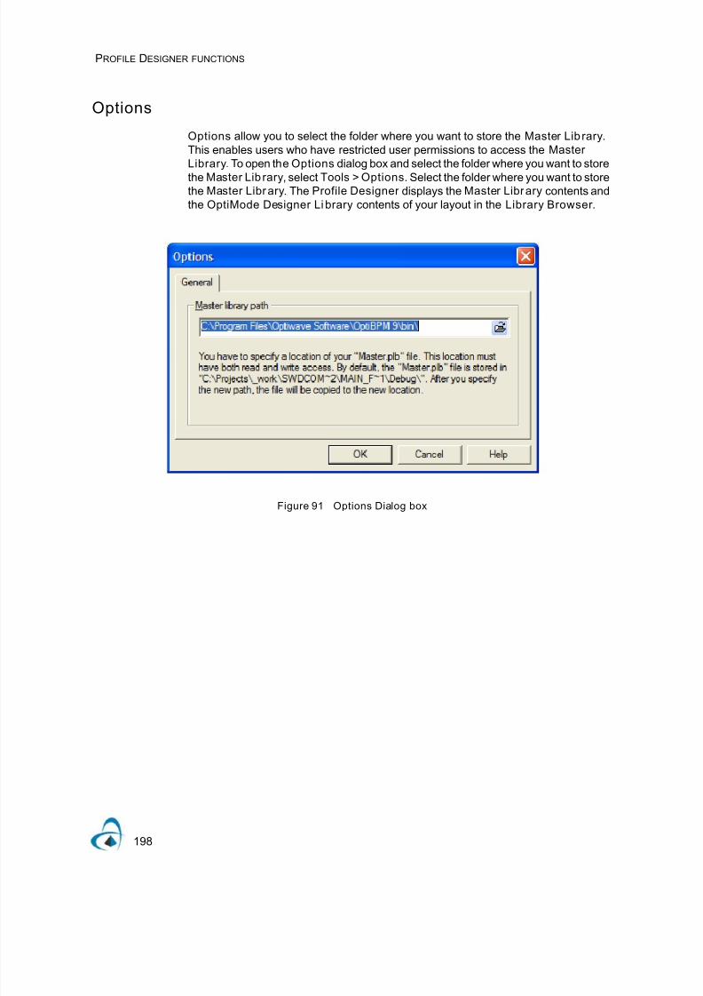
7/21/2019 OptiMode User Reference
http://slidepdf.com/reader/full/optimode-user-reference 202/339
PROFILE DESIGNER FUNCTIONS
198
Options
Options allow you to select the folder where you want to store the Master Lib rary.This enables users who have restricted user permissions to access the Master
Library. To open the Options dialog box and select the folder where you want to store
the Master Lib rary, select Tools > Options. Select the folder where you want to storethe Master Library. The Profile Designer displays the Master Library contents andthe OptiMode Designer Library contents of your layout in the Library Browser .
Figure 91 Options Dialog box

7/21/2019 OptiMode User Reference
http://slidepdf.com/reader/full/optimode-user-reference 203/339
PROFILES
199
Profiles
The waveguide profile defines the index of refraction distribution for waveguides atany point along the length of the waveguide. The positioning of these profiles isdetermined by the positions of the waveguides in the OptiMode designer. Positioningis done relative to the center point of the profile and the center line of the waveguide.The waveguide profile specifies the .center point. of the waveguide. For two-dimensional and three-dimensional waveguides, the profile center point determineshow the waveguide will be positioned in the X direction on a wafer. For three-dimensional waveguides, the center point also determines how the waveguide will bepositioned in the Y direction of the wafer (i.e. the depth of the waveguide in the wafer).Waveguide profiles can be scaled in width and height.
Channel Prof ile
The Channel Profile allows you to create channel waveguides. In its 3Drepresentation, a Channel Profile may be as simple as a single layer (channel) of aselected material, or it can be a complex stack of multiple layers of differentthicknesses, widths, and materials. The Channel Profile "center point" is located at thebottom of the Profile window, at the base of the first layer. The other layers are stackedon top of the previous one, adding to the height of the structure. To open the Channel
Layout dialog box, right-click on the Channel folder in the Master list and select New.

7/21/2019 OptiMode User Reference
http://slidepdf.com/reader/full/optimode-user-reference 204/339
PROFILES
200
Figure 92 Profile Designer - Channel Layout window

7/21/2019 OptiMode User Reference
http://slidepdf.com/reader/full/optimode-user-reference 205/339
PROFILES
201
Channel Profile toolbar
Profile name: Name used to distinguish the current profile from others you maydefine. This name can also be used to access a profile from scripting.
Default: Set the default profile / material used for new projects. Any default in theMaster List will automatically go into the project list at creation time.
2D Profi le Defini tion
Material: The materials have various definitions appropriate for each of the possiblesimulations to be applied. When a 2D simulation is performed, the simulator will usethe 2D definition of the material named in this field. You may want to define the 2Drefractive index by applying Effective Index Theory, rather than a physical refractiveindex here. Select a material from the drop-down list. The material you select is usedwhen the profile is accessed by a 2D Simulation.
3D profi le defini tion
In 3D, the material accessed is the physical refractive index. If the simulation isisotropic, the value in the 3D Isotropic tab of the material is used. If it is anisotropic,the permittivity tensor anisotropic found in the 3D Anisotropic tab of the material is
used. If the material is isotropic but the anisotropic simulator is called, the appropriatediagonal permittivity tensor found by default in the 3D Anisotropic tab of the materialis used. In 3D, more than one layer is possible, so for each layer, a width andthickness is specified. In addition, each layer can be offset from the center line by anarbitrary distance, if required.
For example, consider the following Channel Profile data:
Name Toolbar Button Description
Store Click to save any unsaved settings into the library.
Default Return object settings to their creation time values.
Sync Click to highlight the library item you are working on and synchronize the
current view with an entry in the browser control.
Cancel Click to cancel any unsaved changes and close the current view.
Help Click to access on-line help.

7/21/2019 OptiMode User Reference
http://slidepdf.com/reader/full/optimode-user-reference 206/339
PROFILES
202
Table 2: Channel Prof ile Example InP Rib
When this channel is put on a substrate of material in InPClad with a cladding of air,the cross section (transverse, or x-y plane) refractive index distribution looks like thatshown below.
Figure 93 Refractive Index dist ribu tion for channel profile example
Layer Name: Assigns a name to a layer. Layer names can be used during scripting.Each layer must have a unique name.
Width: Width (x direction) of the channel layer.
Thickness: Thickness (y direction) of the channel layer.
Offset: Layer offset from center line.
Material: Material of the channel layer.
Move Up: Navigates the layer list box.
Layer Name Width Thickness Offset Material
Bottom Clad 5 1 0.0 InPClad
Active Layer 4 0.6 -0.5 InGaAsp
Top Clad 3 2 -1.0 InPClad

7/21/2019 OptiMode User Reference
http://slidepdf.com/reader/full/optimode-user-reference 207/339
PROFILES
203
Move Down: Navigates the layer list box.
Remove: Click to remove a layer.
Add: Click to add a new layer to the 3D profile definition. Enabled only when there is
data for the layer name, width, thickness, and offset. Apply: When making changes to existing layers, click to register changes. This optionis enabled when changes have been made to an existing layer.
Clear: Click to clear all unsaved changes.
Slanted Walls on waveguide profiles Feature
The usual channel waveguide has sidewalls perpendicular to the substrate.Sometimes the manufactured shape is more like a trapezoidal shape, the angle of thetwo walls may be any angle. In Channel Waveguide Profile in the Profile Designer,fields for two angles have been added, the inclination of the right and left sidewall. Bydefault, those angles are degrees. For example, the following channel profile has
the slanted walls checkbox enabled, with as the left angle and as the rightslant angle.
Figure 94 Channel Waveguide Dialog box
The following picture shows how the rectangular channel profile is modified afterapplying the slant angles.
90°45° 60°
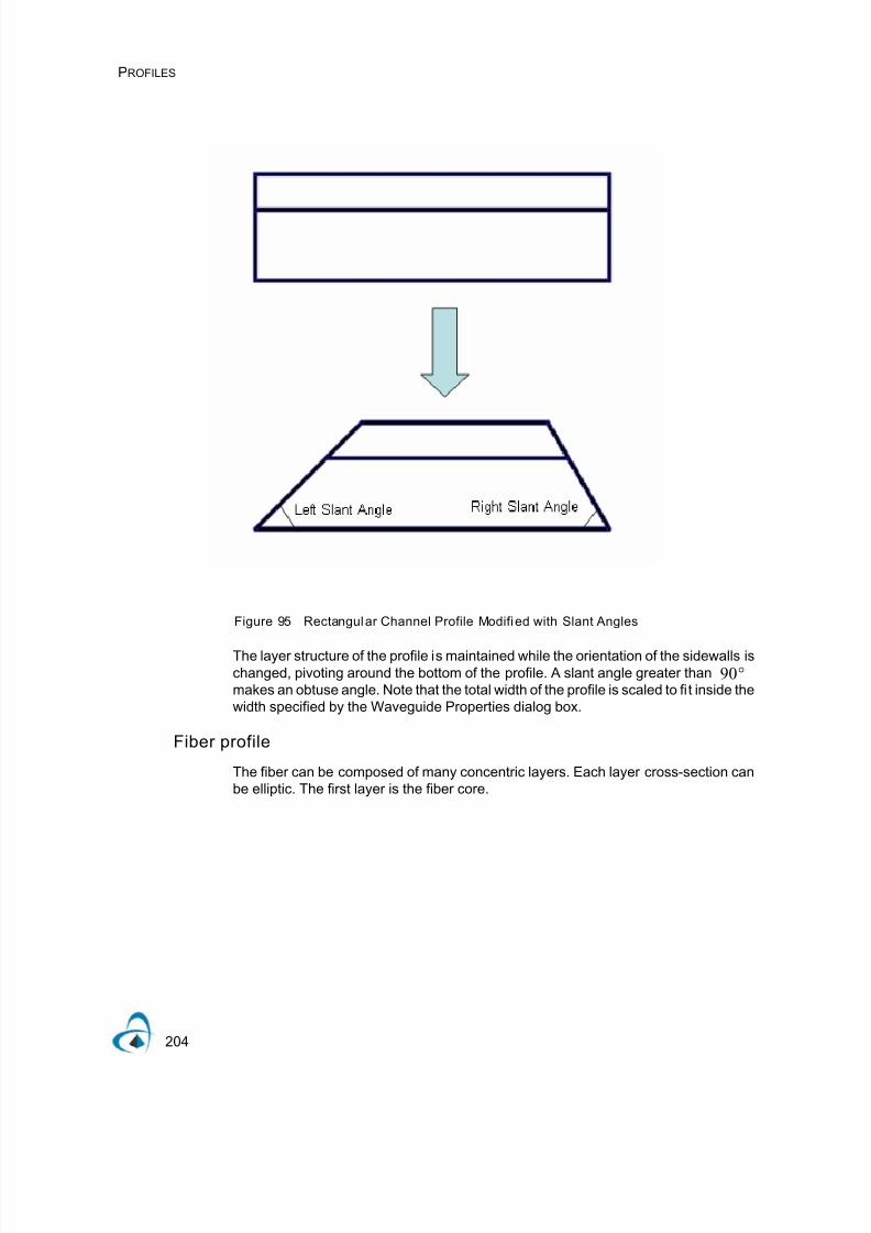
7/21/2019 OptiMode User Reference
http://slidepdf.com/reader/full/optimode-user-reference 208/339
PROFILES
204
Figure 95 Rectangular Channel Profile Modified with Slant Angles
The layer structure of the profile is maintained while the orientation of the sidewalls ischanged, pivoting around the bottom of the profile. A slant angle greater thanmakes an obtuse angle. Note that the total width of the profile is scaled to fit inside thewidth specified by the Waveguide Properties dialog box.
Fiber profile
The fiber can be composed of many concentric layers. Each layer cross-section canbe elliptic. The first layer is the fiber core.
90°

7/21/2019 OptiMode User Reference
http://slidepdf.com/reader/full/optimode-user-reference 209/339
PROFILES
205
Figure 96 Fiber Elliptic Layers
To open the Fiber Profile dialog box, right-click on the Fiber folder in the Master list,and select New.

7/21/2019 OptiMode User Reference
http://slidepdf.com/reader/full/optimode-user-reference 210/339
PROFILES
206
Figure 97 profi le
Fiber Pro toolbar
See the “Channel Profile toolbar” on page 201
Relative semi-axesTo each layer you assign semi-axes of its elliptic shape: Rx and Ry. The semi-axes‘dimensions are related to the physical dimension of the fiber width. For example,Rx=1 means that the semi-axis in the x-direction is equal to the fiber width.
Refractive Index
Each layer has a complex refractive index assigned to it.
Profile name: Name used to distinguish the current profile from others you maydefine. This name can also be used to access a profile from scripting.
2D profi le defini tion
Material: The materials have various definitions appropriate for each of the possiblesimulations to be applied. When a 2D simulation is performed, the simulator will usethe 2D definition of the material named in this field. You may want to define the 2Drefractive index by applying Effective Index Theory, rather than a physical refractiveindex here.

7/21/2019 OptiMode User Reference
http://slidepdf.com/reader/full/optimode-user-reference 211/339
PROFILES
207
Select a material from the drop-down list. The material you select is used when theprofile is accessed by a 2D Simulation.
3D profi le defini tion
The 3D profile definition window displays the layer name, semi-axes Rx, Ry, andmaterial that you select.
Layer Name: Assigns a name to a layer. Layer names can be used during scripting.Each layer must have a unique name.
Rx: Semi-axis size in x-direction of the fiber layer.
Ry: Semi-axis size in y-direction of the fiber layer.
Material: One of the existing Dielectric materials. This will determine the RefractiveIndex in this layer of the fiber.
Remove: Click to remove a selected layer.
Add: Click to add a new layer to the 3D profile definition. Enabled when there is datafor the Layer name, Rx, Ry, and Material.
Apply: When making changes to existing layers, click to register changes. Apply isenabled when changes to an existing layer have been made.
Note: To modify an existing layer, select an existing layer from the layer list, thenmodify either the layer name Rx, Ry or materials controls.
Clear: Click to clear all unsaved changes.
Note: If a layer is not named, it will be reported as an error.
Diffusion process library
Index profiles produced by the default processes are derived from classical diffusionmodels. For other custom index profiles, you can use a built-in formula interpreter thataccepts mathematical expressions. The formula interpreter (string parser) is apowerful tool to design waveguides and devices. The definition of a refractive indexdistribution is as easy as writing the refractive index as a function of the transversalcoordinates, x and y, and a number of the process parameters. For the cross-sectional structure of the waveguides, we assume that it is determined by the diffusionprocess that produces graded refractive index profiles. The index gradation dependson parameters concerning materials, temperature, and the duration of the diffusion.You can control the graded profiles by manipulating the diffusion parameters or, moredirectly, by defining custom profiles.
The following processes are available:
• Ti: LiNb03 profile - Titanium diffusion in lithium niobate
• Mg: LiNb03 profile - Magnesium diffusion in lithium niobate
• H+:LiNb03 profile - Proton Exchange

7/21/2019 OptiMode User Reference
http://slidepdf.com/reader/full/optimode-user-reference 212/339
PROFILES
208
Ti: Linb03 profile - Titanium diffusion in lithium niobate
The titanium diffused waveguides in lithium niobate, or the Ti: waveguidesare formed by the in-diffusion of the titanium dopant into the lithium niobate host. Toform a waveguide, a stripe of titanium is deposited on the substrate. For a
given stripe width, which we identify with the waveguide width, the amount of titaniumis characterized by the stripe thickness before diffusion. The titanium lithium niobatesample is heated for a few hours at temperatures that range from hundreds to athousand degrees Celsius. The titanium ions penetrate the host substrate and form agraded index waveguide. The graded refractive index is a sum of the bulk crystalindex and the diffusion-induced index change .
Where, depending on the crystal cut and light polarization, we consider the ordinary
(o) or extraordinary (e) index distributions. Due to the chromatic dispersion, thegraded index also depends on the wavelength . The diffusion-induced indexchange is described by the product of the dispersion factor and the distributionfunction :
The diffusion-induced distribution function is a function of the distribution constant
, the dopant concentration profile c(x, y) and the distribution power factor ,
The concentration profile can be derived following the classical diffusion theory. Theprofile has a bell-shaped form
In the lateral direction, that is horizontal to the crystal surface, the profile is
characterized by the combination of error functions. In the crystal in-depth direction,
LiNbO 3
LiNbO3
ni
o( )
Δni
ni λ x y, ,( ) ni
o( )λ( ) Δni λ x y, ,( ) i,+ o e,= =
λ( )d i λ( )
hi x y,( )
Δni λ x y, ,( ) d
i λ( )h
i x y,( ) i, o e,= =
F i γi
hi x y,( ) F
ic x y,( )[ ]γi
i, o e,= =
c x y,( ) co
erf w
2 D H
----------- 1 2 x
w
------+
⎝ ⎠
⎛ ⎞ erf w
2 D H
----------- 1 2 x
w
------ –
⎝ ⎠
⎛ ⎞+
⎩ ⎭
⎨ ⎬⎧ ⎫ y
2
DV 2
---------- –
⎝ ⎠
⎜ ⎟⎛ ⎞
exp=

7/21/2019 OptiMode User Reference
http://slidepdf.com/reader/full/optimode-user-reference 213/339
PROFILES
209
that is vertical to the crystal surface, it has a Gaussian shape. The profile's parameters
include the profile constant , the dopant stripe width before diffusion w, the lateral
diffusion length and the diffusion length in depth. In the program, the dopant
stripe width before diffusion is identified with the waveguide width provided by the
layout. The index distribution can be characterized phenomenologically by diffusion
lengths , , or, as an alternative, by diffusion constants , , diffusion
temperature , time and a diffusion temperature coefficient .
To open the Ti: Pro1 window, right-click the Diffusion-Ti: Pro1
folder and select New. The Ti: window allows you to control diffusion of
titanium into lithium niobate.
Figure 98 Titanium prof ile
Ti: Pro toolbar
See the “Channel Profile toolbar” on page 201.
co
D H DV
D H DV DoH DoV
T t T 0 K [ ]
DV
2 tDoV
T o
T ⁄ – ( )exp=
D H
2 tDoH
T o
T ⁄ – ( )exp=
LiNbO3 LiNbO3
LiNbO 3
LiNb03

7/21/2019 OptiMode User Reference
http://slidepdf.com/reader/full/optimode-user-reference 214/339
PROFILES
210
Process definition
Set default: Select to use the default values.
Stripe thickness before diffusion
The thickness of the diffused material stripe before diffusion is used to evaluate thestrength of the diffusion source (total Ti+ ion content).
Group II
Lateral diffusion l ength DH [um] : Diffusion length in the horizontal direction.
Diffusion length in depth DV [um] : Diffusion length in the vertical direction.
Group II
The diffusion lengths in horizontal and vertical directions can be calculated directlyfrom the diffusion process parameters and constants contained in I:
Diffusion temperature Temperature of the diffusion process.
Temperature coeffi cient Constant determines the temperature dependenceof the diffusion lengths.
Diffusion time [Hours]: Time of the diffusion process. Enter the diffusion timein hours, with fractions in the decimal notation.
Diffusion constants, : Constant determines the temperaturedependence of the vertical diffusion length .
Diffusion constants ]: Constant determines the temperaturedependence of the horizontal diffusion length .
Dopant constantThis is a material parameter determined by the dopant density and atomic weight
. The dopant constant is obtained as:
where is the Avogadro number. In caseof which gives cm 5.67. . Thedopant constant is used to calculate the diffusion profile constant in theconcentration profile :
where d is the thickness of the diffused material stripe before diffusion.
c
o
[ ]T 0 K [ ]
t
DoV cm2
s ⁄ [ ] DV
DoH cm2
s ⁄ [ ] D H
cm 3 –
[ ] ρmat – cm
cm
ρ M at
⁄ ( ) N A
=
N ATi ρ, 4.51g cm
3 ⁄ M at , 47.9g mol ⁄ = = 1022
cm 3 –
c0
c x y,( )
c0
dcm
Dv
π--------------=

7/21/2019 OptiMode User Reference
http://slidepdf.com/reader/full/optimode-user-reference 215/339
PROFILES
211
Dispersion factor
:Dispersion factor for the ordinary refractive index.
: Dispersion factor for the extraordinary refractive index.
where is the wavelength in microns.
Distribution constant
: Distribution constant for the ordinary refractive index. The default valueis:
: The distribution constant for the extraordinary refractive index. Thedefault value is:
Distribution power factor
: Distribution power factor of the ordinary refractive index. The defaultvalue is: .
: Distribution power factor for the extraordinary refractive index. Thedefault value is: .
d o
d o
λ( ) 0.67λ2
λ2
0.13 –
----------------------=
d e
d e
λ( ) 0.839λ2
λ2
0.0645 –
----------------------------=
λ
Fo cm3 – [ ]
F o 1.3 10 25 – × cm3=
Fe cm3 – [ ]=
F e
1.2 10 23 –
× cm3
=
Gamma o
γo 0.55=
Gammae
γe 1.0=
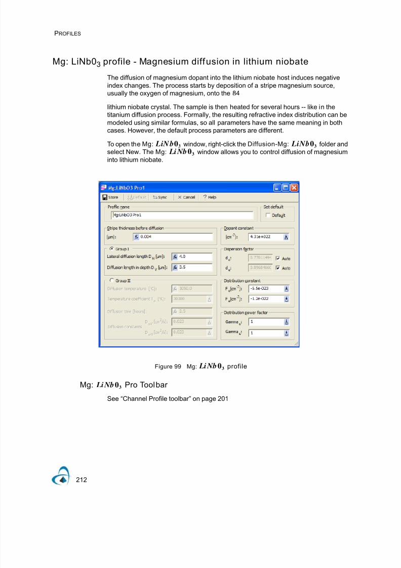
7/21/2019 OptiMode User Reference
http://slidepdf.com/reader/full/optimode-user-reference 216/339
PROFILES
212
Mg: LiNb03 profile - Magnesium diffusion in lithium niobate
The diffusion of magnesium dopant into the lithium niobate host induces negativeindex changes. The process starts by deposition of a stripe magnesium source,usually the oxygen of magnesium, onto the 84
lithium niobate crystal. The sample is then heated for several hours -- like in thetitanium diffusion process. Formally, the resulting refractive index distribution can bemodeled using similar formulas, so all parameters have the same meaning in bothcases. However, the default process parameters are different.
To open the Mg: window, right-click the Diffusion-Mg: folder andselect New. The Mg: window allows you to control diffusion of magnesiuminto lithium niobate.
Figure 99 Mg: profile
Mg: Pro Toolbar
See “Channel Profile toolbar” on page 201
LiNb03 LiNb03
LiNb03
LiNb03
LiNb03

7/21/2019 OptiMode User Reference
http://slidepdf.com/reader/full/optimode-user-reference 217/339
PROFILES
213
Process definition
Stripe thickness before diffusion: The thickness of the diffused material stripebefore diffusion is used to evaluate the strength of the diffusion source (total Mg+ ioncontent).
Group I
See field description in “Group II” on page 210.
Group II
See the field description in “Group II” on page 210.
Dopant constant
This is a material parameter determined by the dopant density and atomic weight. The dopant constant is obtained as:
where is the Avogadro number. The dopant constant is used to calculate thediffusion profile constant in the concentration profile :
where d is the thickness of the diffused material stripe before diffusion.
Dispersion factor
See field description in .“Dispersion factor” on page 211.
Distribution constant
:Distribution constant for the ordinary refractive index. the default value is:
:Distribution constant for the extraordinary refractive index. the defaultvalue is:
cm3 – [ ]
ρ M at
cm
cm
ρ M at
⁄ ( ) N A
=
N Ac0 c x y,( )
c0
dcm
DV
π---------------=
F o cm3 – [ ]
F o
5.5 10 23 –
× cm3
– =
Fe cm3 – [ ]
F e
1.2 10 22 –
× cm3
– =

7/21/2019 OptiMode User Reference
http://slidepdf.com/reader/full/optimode-user-reference 218/339
PROFILES
214
Distribution power factor
: Distribution power factor of the ordinary refractive index. The defaultvalue is: .
Gammae: Distribution power factor for the extraordinary refractive index. The defaultvalue is: .
H+:LiNb03 profile - Proton Exchange
Proton exchange in lithium niobate involves a replacement of lithium ions, Li+, byhydrogen ions, or protons, H+. The replacement causes a change in refractive index,thus forming a waveguide. Proton exchange is one of the methods used for formingoptical waveguides in lithium niobate, LinbO3, as well as in lithium tantalite, LiTaO3.The waveguide formation can have two stages. Basic proton exchange takes placewhen the lithium niobate substrate is immersed in an appropriate proton source,usually an acid melt, and heated for a couple of hours at temperatures ranging from150 to 300 degrees Celsius. Under these conditions, the two ion species counter
diffuse, so that material is exchanged between the substrate and the melt. To openthe Proton Exchange window, right-click the Diffusion—Proton Exchange folderand select New. The Proton Exchange window allows you to control the protonexchange diffusion process.
Figure 100 Proton Exchange prof ile
Gamma o
γo 1.0=
γe 1.0=

7/21/2019 OptiMode User Reference
http://slidepdf.com/reader/full/optimode-user-reference 219/339
PROFILES
215
Proton Exchange toolbar
See the “Channel Profile toolbar” on page 201
Process definition
Annealing process
No: No annealing will be applied.
Yes: Annealing process will be applied to calculation of diffusion profile.
Parameters button : Click Parameters to open the Anneal ing Process dialog box.For more information see “Annealing process” on page 215.
Note: The Parameters button will only become available if the Yes radio buttonhas been selected.
Diffusion depth before annealing
The diffusion depth before annealing can be user defined or automatic. The Auto
option requires specifying the proton source, the process time and temperature. In thecase of a user proton source, the diffusion constant, and activation energy should bespecified.
Au to: If you clear the Auto check box, you can enter data in the edit box.
Proton source
The three available proton sources are:
• Toluic Acid
• Benzoic Acid• User source
Note: Selecting User Source will activate the Exchange Edit boxes.
Process parameters
Parameters that determine changes of the refractive index profile after the protonexchange process.
Time [hours]: Duration of the exchange process.
Temperature [oC]: Temperature of the exchange process.
Exchange
Diff. Constant : Characterizes the exchange process.
Acti vat . Energy KJ / mol : Influences the diffusion depth of the process.
μ m2
h ⁄ [ ]
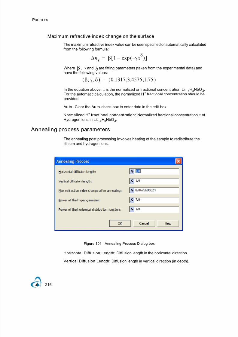
7/21/2019 OptiMode User Reference
http://slidepdf.com/reader/full/optimode-user-reference 220/339
PROFILES
216
Maximum refractive index change on the surface
The maximum refractive index value can be user specified or automatically calculatedfrom the following formula:
Where , and are fitting parameters (taken from the experimental data) andhave the following values:
In the equation above, x is the normalized or fractional concentration Li1-xHxNbO3.For the automatic calculation, the normalized H+ fractional concentration should beprovided.
Au to: Clear the Auto check box to enter data in the edit box.
Normalized H+ fractional concentration: Normalized fractional concentration x ofHydrogen ions in Li1-xHxNbO3.
Annealing process parameters
The annealing post processing involves heating of the sample to redistribute thelithium and hydrogen ions.
Figure 101 Annealing Process Dialog box
Horizontal Diffusion Length: Diffusion length in the horizontal direction.
Vertical Diffusion Length: Diffusion length in vertical direction (in depth).
Δns β 1 γ xδ
– ( )exp – [ ]=
β γ δ
β γ δ, ,( ) 0.1317 3.4576 1.75;;( )=

7/21/2019 OptiMode User Reference
http://slidepdf.com/reader/full/optimode-user-reference 221/339
PROFILES
217
Max. Refractive Index Change after Annealing: Maximum change of the surfacerefractive index after annealing.
Note: Only the extraordinary refractive index is considered to be modified by theproton exchange process.
Power of the Hyper-Gaussian: Power of the Hyper-Gaussian refractive indexdistribution function f(y) in the vertical (in depth) direction.
Power of the Horizontal Distribution Function: Power of the horizontal refractiveindex distribution function.
User Defined Profiles
The User Defined Profiles provide huge flexibility in waveguide creation. With a
custom defined function, you can dictate the refractive index value at any given pointwithin the waveguide's cross-section.
When designing the Profile Function, you may choose:
• User Function profile
• User DLL profile
The User Function profile is based on the programs internal expression parser. It is asimple interpreter of single-line expressions. It is particularly useful when working withsimpler refractive index distribution schemes. The User DLL profile is based on anexternally compiled binary DLL. With this approach, you can develop complexrefractive index distribution schemes. In a practical sense, the results depend only on
the compiler and the programming skills of the user. Performance wise, this solutionis much faster than the expression parser based one. The following sections providea description of the concept and its applications.
Definit ion of user defined profiles
The concept of the User Defined profiles is constructed around a user-definedfunction. The function definition consists of the following elements:
• Function declaration
• Function body
• Function domain (limits)
You can arbitrarily specify each of the above elements.Profile Name: Each of the profiles has to be assigned a unique name. The sameapplies to the User Defined profiles. The Profi le Name is an independent identity, andit may but does not have to have the same name as the Profile Function. Differentprofiles (distinguished by their names) can be assigned the same Profile Function.
f y( ) y
Dv
------⎝ ⎠⎛ ⎞ a
– exp=

7/21/2019 OptiMode User Reference
http://slidepdf.com/reader/full/optimode-user-reference 222/339
PROFILES
218
Types of user defined profi les
User Defined profiles may be additive or overwriting. You can select whether a UserDefined profile is overwriting or additive.
Addi ti ve pro fi leThe additive profile behaves like a diffusion process. The profile functions return valueis added to the underlying refractive index value at the specified mesh-point:
n(x,y) = n0(x,y)+ProfileFunction(arg1, arg2, arg3, …, argN)
Where n0(x,y) is the value of the refractive index at the x,y mesh point.
Overwriting profile
The overwriting profile behaves as a channel or fiber profile, i.e., the profile functionreturn value overwrites the underlying value of the refractive index at the specifiedmesh-point:
n( x, y) = Prof i l eFunct i on( ar g1, arg2, arg3, …, argN)
Function declaration
The function definition has the following form:
FunctionName (arg1, arg2, arg3, …, argN )
The FunctionName is a function name declarator. Its construction conforms to thefollowing rules:
• It can consist of any letters of the English alphabet, digits 0 -9, and an
underscore
• It has to start with a letter or underscore
• It is case sensitive
The profile Function Name is internal to the profile, i.e., it is not visible to otherfeatures of the software.
The arguments are defined by their names. The arguments are given by name only,without the type specification. The type is always double precision (float) variable.There is no limit on the number of the function arguments.
Function arguments
You may specify any number of arguments in the function declaration. The argumentsmust be unique, i.e., their names cannot be repeated. The function arguments areutilized in the function body to perform calculations of a refractive index value.Externally to the function, the function arguments are simply placeholders. During theruntime execution they will be assigned values that are transferred into the function.The arguments are passed to the function by value, i.e., after the function returns fromthe call, their values are preserved. Therefore, they cannot be used to transfer resultsof the function execution from the function. You can impose validity ranges on thefunction arguments. The range settings are always inclusive, i.e.:

7/21/2019 OptiMode User Reference
http://slidepdf.com/reader/full/optimode-user-reference 223/339
PROFILES
219
Lower Li mi t <= Ar g <= Upper Li mi t
When an argument value is beyond the specified range, the value returned by thefunction is discarded, or the function is not executed at all.
Argument associationsTo define the relationship between particular function arguments and SystemVariables, the parameter must be associated with one of the predefined SystemVariables. OptiMode currently supports a set of System Variables that track things likethe current width of the waveguide and the distance of the current mesh point fromthe center of the waveguide. The values assigned to the arguments originate from theset of predefined System Variables and the User-Defined Variables. You canassociate any of the System Variables and/or your own previously defined variablesto any of the function arguments. The same System Variable and/or User DefinedVariable can be associated with (assigned to) any number of function arguments.
Note: All of the Profile Function arguments must be associated with a system or
user variable.
System Variables
Each time an index of refraction value is needed from a User Defined Profile,OptiMode evaluates all of the required system variables, assigns the System Variablevalue to the associated argument, and calls the function to calculate the index ofrefraction value.
Polarization
Name: _Polariz
Polarization is a simulation parameter. The parameter can have one of the following
values:• TE = 0
• TM = 1
In case of the 3D Isotropic simulations without polarization (Scalar solver), _Polarizhas the value of TE polarization.
Distance from the nearest waveguide
Name: _d
This parameter is layout (mask) dependent. It carries information about a distancefrom the nearest waveguide with the same profile (or process). The waveguides have
to have the same User Profile (the same Profile Name). It is primarily used whencalculating the contribution of the nearest waveguide's mask-window to the currentwaveguide's diffusion process. Most of the time _d is used in conjunction with the _W1parameter. The value is calculated with respect to the waveguide's centers. It isdifferent for the mesh points positioned on the left and the right side of the currentwaveguide, since it refers to the neighbour waveguides positioned on the same sideof the waveguide center as the mesh points under consideration.

7/21/2019 OptiMode User Reference
http://slidepdf.com/reader/full/optimode-user-reference 224/339
PROFILES
220
The value of this parameter for the points located at the center of the waveguide isequal to the smaller value of the distance from either of the neighbouring waveguides.Its value is equal to "infinity", i.e., the maximum value of the double precision number,
if there is no other waveguide in the neighbourhood.
Width of the nearest waveguide
Name: _W1
This parameter is layout (mask) dependent. It carries information about the width ofthe nearest waveguide. The neighbour waveguide profile has to be the same. Thewaveguides have to have the same User Profile (the same Profile Name). It isprimarily used when calculating the contribution of the nearest waveguide's maskwindow to the current waveguide's diffusion process. Most of the time _W1 is used inconjunction with the _d parameter. The value is different for the mesh pointspositioned on the left and the right side of the current waveguide. It is the same for allpoints positioned on the same side of the waveguide centerline.
The value of this parameter for the points located at the center of the waveguide isequal to the width of the closest of the neighbouring waveguides, i.e., the smallest _dparameter. The value is equal to zero if there is no other neighbouring waveguide.
Dependency of the diffusion additi ve Profi le processes on the Neighbouringwaveguides
With diffusion processes, their contribution to the refractive index distribution extendsbeyond the waveguide's mask-window, i.e., beyond the waveguide shape. Theseprocesses are additive by nature. This can create problems when calculatingrefractive index contributions coming from two waveguides positioned close to eachother (see below).
In order to achieve the realistic (desired) refractive index distribution, the diffusionprocess implementation will utilize dependency on _d and _W1.
Distance from the waveguide center
Name: _dx
This parameter carries the value of the mesh-point distance from the center of thewaveguide in the horizontal direction. It is always positive. It is equal to zero for allmesh-points located at the waveguide centerline.
Signed distance from the waveguide center
Name: _sdx
This parameter carries the value of the mesh-point position in a local coordinatesystem with the center at the centerline of the waveguide cross-section. The mostimportant difference between _sdx and _dx is the sign:
• _dx is positive for mesh points on the right side of the waveguide centerline
• _dx is equal zero for mesh-points located at the waveguide centerline
• _dx is negative for mesh points on the left side of the waveguide centerline

7/21/2019 OptiMode User Reference
http://slidepdf.com/reader/full/optimode-user-reference 225/339
PROFILES
221
Distance from the waveguide surface
Name: _dy
This parameter carries the value of the mesh-point distance from the waveguidesurface in depth. It is always positive. It is equal zero for all mesh-points located onthe waveguide surface. The surface of the waveguide is the same as the top of theUser Defined Profile, i.e., it is equal to the depth of the waveguide. The value of theparameter is calculated for all the mesh-points of the calculation space located belowthe waveguide surface level, i.e., for the full extent of the wafer width, not just underthe waveguide's mask-window. The parameter value is not calculated for the mesh-points located above the waveguide surface.
Note: The _dy variable is equal to zero for 2D simulations. As a result, profilesutilizing the depth of the mesh-point ( _dy) information, typically 3D simulations canalso be used in 2D simulations. It is assumed that the depth of all the mesh points isequal to zero, i.e., the top of the waveguide (profile) surface.
Waveguide width
Name: _W
This parameter carries the value of the waveguide's. All of the mesh points, positionedunder the Profile‘s surface level, will be passed the value of the _W parameter.
Coordinates of a mesh point i n the global coordinates system
Name: _x, _y, _z
These parameters carry the values of particular mesh-points in the global (wafer)coordinate system.
Wavelength
Name: _Wavelen
This parameter carries the value of the wavelength simulation parameter. If thewavelength is assigned a user defined variable, which is varied across the simulations(VB Script), the _Wavelen system variable will contain the actual value of theparameter assigned by VB Script.
Access to opt ical f iel d values
Name: _Emod, _EE, _Eim, _Ere
These parameters carry the values of the currently simulated optical field at aparticular mesh-point. The optical field at any point is represented by a complex
number. The specified parameters carry values derived from the optical fieldcomponent. These parameters are useful when calculating the influence of the opticalfield on the refractive index distribution, i.e., non-linear effects.
The meaning of the parameters:
_Emod: The Ampl i t ude of t he opt i cal f i el d at t hepar t i cul ar mesh poi nt .

7/21/2019 OptiMode User Reference
http://slidepdf.com/reader/full/optimode-user-reference 226/339
PROFILES
222
sqrt(_Ere2+ _Ei m2)
_EE: The I nt ensi t y of t he opt i cal f i el d at t he part i cul armesh poi nt :
_Ere
2
+ _Ei m
2
_ Eim : The I magi nar y par t of t he opt i cal f i el d componentat t he par t i cul ar mesh poi nt .
_Ere: The Real par t of t he opt i cal f i el d component at t hepar t i cul ar mesh poi nt .
Function body execution
The function body contains execution code that calculates the value of the refractiveindex for the provided set of arguments. Specification of the function body dependson the selected solution. Currently, two approaches have been defined:
• Support by the internal single line expression Parser
• Support by a DLL
The function code is executed only for the selected subset of the mesh points, fulfillingthe following conditions:
• The mesh point has to be located below or at the surface level of the UserDefined Profile. The position of the User Defined Profile level is equal to theWaveguide Depth.
• The mesh point has to be located on the mesh grid intersecting thewaveguide shape.
The above conditions mean that the mesh points located on the vertical grid-cut lines,perpendicular to the propagation direction, and intersecting the waveguide shape,
may be affected by the function calculation results.
However, the function will not be executed for mesh points located before and afterthe waveguide shape.
Function domain (Limits)
During a simulation, the User Defined Profile provides an index of refraction value foreach simulation mesh point within the 'domain' of the profile. The 'domain' of theprofile is that region within the simulation that is influenced by the profile. This domaincan extend beyond the width of the waveguide. The domain of the profile function isalso called the Limits. If the mesh point is within the domain of the profile, then theProfile Function will be asked for a refractive index value for that mesh point, and the
returned value will be applied to this mesh point. If the mesh point is outside thedomain of the profile, then the Profile Function return value will be discarded, and nochanges will be made to the mesh point‘s value. The Function Domain or FunctionLimits determines where the function solution is applicable. The Function Limit is afunction (expression), which returns:
0 - for the areas where the functional response is invalid, i.e., the functiondoes not (is not supposed to) exist

7/21/2019 OptiMode User Reference
http://slidepdf.com/reader/full/optimode-user-reference 227/339
PROFILES
223
1 - for the areas where the functional response is valid
The main task of the Limit function is to validate provided argument values in afunctional dependency and determine whether the Profile Function should beexecuted, or its value accepted. The classical definition of the function domain relies
on the limits imposed on the function arguments. However, this definition does notprovide sufficient functionality. In order to overcome this limitation the FunctionDomain concept has been introduced. The practical purpose of the Limit function isto provide tools that allow definition of geometrical limits/patterns on refractive indexdistribution.
User Function Profile
OptiMode is equipped with an internal Expression Parser. The parser is able to parsesingle line expressions. It supports the definition of variables and functions that canbe created with a single line expression. The User Function Profile construct is atypical Expression Parser supported function:
Function declaration: FunctionName( arg1, arg2, arg2, …, argN)
Function expression: Single line mathematical expression returning a doubleprecision value of refractive index
Function limit: Single line mathematical expression returning a double value equal1.0 Or 0.0:
• Return value of 1.0 means that the function results are valid and within itsdomain
• Return value of 0.0 means that the function results are invalid and should bediscarded
The internal expression parser provides means to define simpler refractive index
distribution profiles. The profile function can get more complex when it is implementedwith use of the other user implemented (defined) functions and variables. However,this becomes more cumbersome for involved solutions.
The execution of the profile functions based on the internal parser is much slower thanthe compiled code (DLL), since the internal parser is a simplified interpreter.
User funct ion profile - Function declaration
The function definition must be provided in the following form:
FunctionName (arg1, arg2, arg3, …, argN )
The FunctionName is a function name declarator. Its construction conforms to thefollowing rules:
• It can consist of any letters of English alphabet, digits 0 -9, and an underscore
• It has to start with a letter or underscore
• It is case sensitive
7/21/2019 OptiMode User Reference
http://slidepdf.com/reader/full/optimode-user-reference 228/339
PROFILES
224
The Profile Function Name is internal to the Profile, i.e., it is not visible to otherfeatures of the software. The arguments are defined by their names. The argumentsare given by name only, without the type specification. The type is always a doubleprecision (float) variable. There is no limit on the number of the function arguments.
User function profile—Function body
The function body is constructed as a single-line expression. When constructing thefunction expression, you may use any of the following elements:
• Predefined Expression Parser supported functions
• Predefined Expression Parser supported constants
• The user defined variables and functions
• Any of the function arguments
For more information on parser supported functions and constants, see .Appendix C:Parser supported functions. on page 167. You cannot use (reference) any otherProfile Function, i.e., by their Profile Function Name or the Profile Name.
When constructing the function expression, you should have full access to the UserVariables and Functions:
• Add and remove variables and functions
• Modify existing variables and functions
• View and observe their values
The result of function body execution is a double value used to determine the functioncontribution to the refractive index distribution.
User function profile—Function limit
The Function Limit is an expression. The expression is of the same type as that of themain function body. When constructing the Function Limit expression, you can use
_FnRslt. The _FnRslt is a reserved variable, which carries the result value of the mainfunction expression execution. This variable can be used in the Limit expression tocarve-out of the function domain areas based on the "amplitude clipping" of thefunction return values. The Function Limit expression operates on the same set offunction arguments as the main Profile Function. Simply the arguments specified inthe main function declaration are passed to its Limit function for evaluation, during theexecution. This dependency can be illustrated as follows:
If the Profile Function declaration is ProfileFunction( arg1, arg2, arg3, …, argN ),then the Profile Function expression would be LimitFunction( _FnRslt , arg1,
arg2,arg3, …, argN )
The declaration of the Limit Function is hidden from the user, as you can only dictatethe implementation of the Limit Function expression. However, you can use any of thearguments of the Profile Function declaration in the expression.
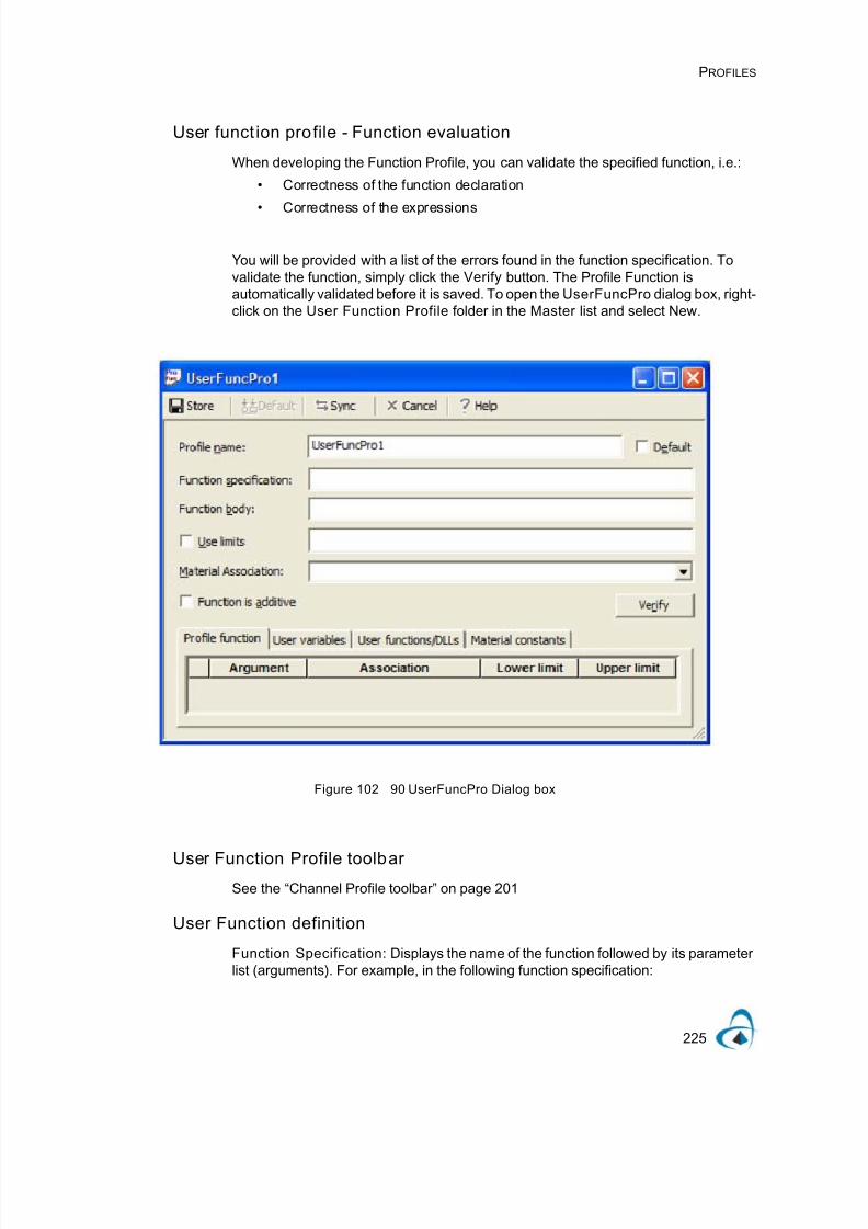
7/21/2019 OptiMode User Reference
http://slidepdf.com/reader/full/optimode-user-reference 229/339
PROFILES
225
User funct ion profile - Function evaluation
When developing the Function Profile, you can validate the specified function, i.e.:
• Correctness of the function declaration
• Correctness of the expressions
You will be provided with a list of the errors found in the function specification. Tovalidate the function, simply click the Verify button. The Profile Function isautomatically validated before it is saved. To open the UserFuncPro dialog box, right-click on the User Function Profile folder in the Master list and select New.
Figure 102 90 UserFuncPro Dialog box
User Function Profile toolbarSee the “Channel Profile toolbar” on page 201
User Function definition
Function Specification: Displays the name of the function followed by its parameterlist (arguments). For example, in the following function specification:

7/21/2019 OptiMode User Reference
http://slidepdf.com/reader/full/optimode-user-reference 230/339
PROFILES
226
MyFunction(x,y), MyFunction is the function name, and x,y is the parameterlist (arguments).
Function Body: The function is defined by any single line mathematical equation thatcan be parsed by the OptiMode parser. For more information, see .Appendix C:
Parser supported functions. on page 167. The formula can contain the functionarguments, existing user variables and functions, and system and material constants.When defining a function body, the arguments do not have numerical values. Thefunction is not evaluated even if you express it with the help of well defined additionalparameters and user variables having numerical values. The function definition formsonly a template. The function is evaluated in numerical simulations only after youassign values to the function.
For example, you can define your function as:
MyVar i abl e*Wi dt h*exp( - ( x*x+y*y) )
Width is a parameter equal to 4. MyVariable is a user variable equal to 3. Still,the function value is not determined since the values of x and y is not known.
Use Limits: Select to enable the application of limits on the function arguments andthe function value.
If the box is not selected, the function is evaluated and applied to all the mesh pointsin the whole space below the Profile Surface level, i.e. the waveguide depth. Whenselected, the function input arguments can be limited by specifying a Booleanexpression within the Use limits input box.
For example, enter the expression: x*x+y*y<1, to limit the function domain by acircle of radius 1. You can also limit the function by using the variable _FnRsIt_ ,which is the function value. If you enter the
Limits expression: abs(_FnRsIt_)<1, you ensure that your function is clippedwhen its absolute value is equal or exceeds 1.
Material Association: Select a material from the material database. All theaccessible material constants are associated with the selected material. Ordinary anddiffused materials provide access to different sets of material constants. Ordinarymaterials have only values of the refractive indices, whereas the diffused materialscan also provide values of the permittivity and electro-optic coefficients. If the functionargument is associated with a particular material constant, the constant should returnthe correct value for selected material. For example, you can use the refractiveindices of available materials to define a profile.
Verify: Verifies correct definition of the user function profile, i.e. correct definitions andavailability of used variables and association of the input parameters of the userprofile function.
Note: Verification must be performed before the profile is saved.

7/21/2019 OptiMode User Reference
http://slidepdf.com/reader/full/optimode-user-reference 231/339
PROFILES
227
Function is additive: Select if the refractive index of the created waveguide issupposed to be the sum of the underlying refractive index and the perturbationdefined by the user-defined function:
If Function is additive is not selected, the refractive index profile is non-additive,
i.e., the refractive index of the waveguide is equal to value of the user-definedfunction:
Profile function tab
The Profile function tab specifies the association and limits of the function inputparameters. Every input parameter needs to be associated with a user variable,material, or system constant. Click on the association input field to view a list of all theavailable variables and constants. You can also impose limits on the input argumentsof the user defined profile functions. The values in the lower limit and upper limit inputdirectly limit the values of input arguments. Using limits is not required.
Figure 103 Profile Function tab
User variables tab
The User variables tab displays a list of all the available user variables, which can beused in the construction of user functions. The user variable has a symbolic name(User Variable) and a numerical value determined by an expression (Expression).The expression defining the variable can be a mathematical formula containingexisting parameters, variables, and functions. The variables can be modified withinthe Variables and Functions dialog box (“Variables and Functions dialog box” on page167).
Note: This is a read-only list.
n n0 f umentsarg( )+=
n f umentsarg( )=
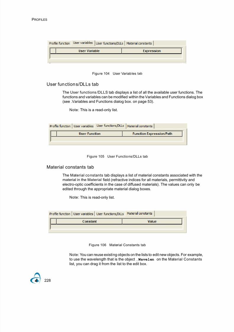
7/21/2019 OptiMode User Reference
http://slidepdf.com/reader/full/optimode-user-reference 232/339
PROFILES
228
Figure 104 User Variables tab
User functions/DLLs tab
The User functions /DLLS tab displays a list of all the available user functions. Thefunctions and variables can be modified within the Variables and Functions dialog box(see .Variables and Functions dialog box. on page 53).
Note: This is a read-only list.
Figure 105 User Functions/DLLs tab
Material constants tab
The Material constants tab displays a list of material constants associated with thematerial in the Material field (refractive indices for all materials, permittivity andelectro-optic coefficients in the case of diffused materials). The values can only beedited through the appropriate material dialog boxes.
Note: This is read-only list.
Figure 106 Material Constants tab
Note: You can reuse existing objects on the lists to edit new objects. For example,to use the wavelength that is the object _Wavelen on the Material Constants
list, you can drag it from the list to the edit box.

7/21/2019 OptiMode User Reference
http://slidepdf.com/reader/full/optimode-user-reference 233/339
PROFILES
229
Example
You want to customize the waveguide index profile according to the formula:
where is the constant substrate refractive index (base index), and the gradedindex variation is the user function. The function arguments, x and y, areusually associated with the local layout transverse coordinates of the waveguide. Inthis example, you define the user function profile MYPROFILE with functionspecification deltaN and function body:
del t aN( x, y) = d*F*C0*( er f ( W/ ( 2*Dx) ( 1+2*x/ W) ) +
er f ( W/ ( 2*Dx)*( 1- 2*x/ W) ) ) *exp( - y*y/ ( Dy*Dy))
Note: In general, the user function can have many arguments. In the aboveexample, the only arguments are x and y, while the remaining symbols d, F, C0,W, Dx and Dy , represent parameters and user variables that are not the functionarguments in the present context. The variables and constants need to be defined
before the profile definition.
Select Function is additive.
In Profile function, make the following association:
x->_dx
y->_dy
Verify and Store the profile.
User DLL profile
The DLL based profiles are designed to provide tools to define complex refractive
index distribution. User DLL profiles provide more flexibility than function definedprofiles, because the profile function is a programmed function located in a DLL -implementation is limited only by the programming skills of the user. The DLL functionis programmed in a C or C++ compiler, and compiled into a DLL. The complexity ofthe User DLL profile is therefore limited by the capabilities of the compiler and thesoftware development skills of the user. If necessary, multiple functions spanningmultiple files can be used to create the profile function. You can build the DLLs withany compiler supporting DLL creation. However, we will focus on supporting only C,C++ (Microsoft) compilers. Use of other compilers may require some experimentationwith compilation and linking options.
User DLL profile - Function declaration
The function definition must be provided in the following form:
FunctionName (arg1, arg2, arg,3, …, argN )
The FunctionName is a function name declarator. Its construction conforms to thefollowing rules:
• It can consist of any letters of English alphabet, digits 0 -9, and an underscore
n x y,( ) no
Δn x y,( )+=
n0
Δn x y,( )

7/21/2019 OptiMode User Reference
http://slidepdf.com/reader/full/optimode-user-reference 234/339
PROFILES
230
• It has to start with a letter or underscore
• It is case sensitive
The Profile Function Name is internal to the Profile i.e. it is not visible to other featuresof the software. The arguments are defined by their names. The arguments are given
by name only, without the type specification. The type is always double precision(float) variable. There is no limit on the number of the function arguments. Thefunction declaration provides the application with the information on the functionexported from the developed DLL. It the user to specify a function located within a DLL(also user specified) that will provide the refractive index distribution. This functionmust be wholly contained within the DLL; it cannot require any data from theapplication with the exception of the current input values for the arguments. It is criticalthat the number of arguments in the function declaration and the functionimplemented within the DLL is the same. The software will crash otherwise. All thearguments of the function implemented in the DLL must be double precision (float)numbers.
User DLL profi le - Location (Function body)
In this case the function has no "body" i.e. implementation within the OptiModeapplication. The whole function code is located inside the DLL. The user has toprovide a path to the location of the DLL where the declared function is implemented.
User DLL profile - Location specification
The user may provide the path to the DLL in few forms, each of these forms willprompt different DLL search pattern. The generic form of the DLL locationspecification:
[Directory path access]\FunctionDllName.dll
Full pathname
The user specifies the full pathname to the DLL. The full pathname specification startswith the drive letter
e.g.:
D:\Optiwave Software\User DLLs\MyRIdxProfile.dll
In this case the application will directly examine the location for presence of thespecified DLL, then verify whether the specified function is exported from the DLL (i.e.whether it is visible from outside of the DLL).
Relative pathname
The user may specify a relative pathname. The relative path name is a partial one: itdoes not contain the drive letter specification, just the directory path. Few examples:
\User DLLs\MyRIdxProfile.dll
MyRIdxProfile.dll
Samples\ MyRIdxProfile.dll
In all these cases the DLL search pattern is the following:

7/21/2019 OptiMode User Reference
http://slidepdf.com/reader/full/optimode-user-reference 235/339
PROFILES
231
• The current directory (folder) is determined based on the processed data file.
• Then the relative DLL pathname is appended to the current directorypathname, and the newly constructed full path is tested for location of the
specified DLL. After the DLL file is located it is verified whether the specifiedfunction is exported from this DLL.
Example
The currently processed data file is located at:
C:\My Documents\OptiModedata.bpd
The relative pathname of the DLL is specified as:
\OptiMode DLLs\MyRIdxProfile.dll
The full path-access to the DLL will be constructed as:
(C:\My Documents\) + (\OptiMode DLLs\MyRIdxProfile.dll)
resulting in the following pathname:
C:\My Documents\OptiMode DLLs\MyRIdxProfile.dll
The path: "C:\My Documents\OptiMode DLLs\" will be verified for presence of the"MyRIdxProfile.dll", and then the DLL will be examined whether it the specifiedfunction is available.
In case the relative DLL's pathname contains just the DLL name, the DLL is expectedto be located in the directory of the currently processed data file. If the previouslysearched location does not contain the specified DLL, the application is going to relyon the operating system DLL search pattern.
User DLL profile - Function limit
The User DLL profiles must be able to specify its domain or limits. This domain isspecified using a DLL defined function. It is declared the same way as the ProfileFunction (see .User DLL profile - Function declaration. on page 99). Limit functionsmust return a =double‘ data type. The function must return 0 for FALSE if the profileshould be ignored for a given mesh point, or 1 for TRUE if the profile must supply arefractive index value for a given mesh point. For example, a limit function might looksomething like:
double mylimit( double x ){
doubl e i ncl ude_t hi s_poi nt = 0;i f ( x==1){
i ncl ude_t hi s_poi nt = 1;}r et ur n i ncl ude_t hi s_poi nt ;
}
By specifying a domain, we can allow the background refractive index value to tightlysurround non-rectangular profile shapes. We also prevent the Function defined profilefrom overwriting everything under it across the entire wafer. (User defined profiles can

7/21/2019 OptiMode User Reference
http://slidepdf.com/reader/full/optimode-user-reference 236/339
PROFILES
232
have influence beyond the waveguide width). Note that we do not have a systemvariable, which would provide the 'background' refractive index value.
The DLL domain (Limit) function is independent from the DLL Profile Function. Itcarries its own set of arguments, which also have to be associated with the system or
user defined variables. If the name of the arguments in the Limit Function is the sameas an argument in the Profile Function, then the arguments are assumed to berepresent the same parameter and only one name will appear on the association listi.e. both arguments will be associated with the same variable.
At tenti on:
The arguments in the function declaration are only the placeholders. They areindependent from actual function argument names in the DLL. What is important isthe number of the arguments and their order.
It is enough to provide a different argument name in the Limit Function to make surethat it can be associated with a distinct variable.
User DLL profile - Function evaluation
After you specify the DLL Function Profile, you may validate the specified function i.e.:
• Correctness of the function declaration
• Existence of the DLL
• Availability of the specified profile function within the DLL
To validate your Profile Function, click Verify, and you will see the errors found in thefunction specification.
To open the UserDLLPro dialog box, right-click on the User Function Profile folderin the Master list and select New.

7/21/2019 OptiMode User Reference
http://slidepdf.com/reader/full/optimode-user-reference 237/339
PROFILES
233
Figure 107 UserDLLPro Dialog box
User DLL Profile toolbar
See “Channel Profile” on page 199.
Profile name: Name used to distinguish the current profile from others you maydefine. This name can also be used to access a profile from scripting.
Default: Set the default profile / material used for new projects. Any default in theMaster List will automatically go into the project list at creation time.
User DLL function definition
Function Specification: Displays the unique name of the function followed bysymbolic arguments.
For example, in the following DLL function specification: MyFunction(x,y), MyFunction is the function name, and x,y are the arguments.
Note: You must provide the exact number of arguments of the DLL function.
DLL File Name: Specifies file name and location of the DLL file. A DLL file containscomputer code specifying the process function. To apply a function defined in theDLL, you must provide the exact name of the DLL function.

7/21/2019 OptiMode User Reference
http://slidepdf.com/reader/full/optimode-user-reference 238/339
PROFILES
234
Material: The Material constant tab displays a list of the parameters of a materialdefined in the Material input box.
Verify: Verifies the definition of the user DLL profile, i.e. looks for correct definitionsand association of the input parameters of the user profile function.
Note: Verification must be performed before the profile is saved.
Function is additive: See definition in “User Function definition” on page 225
Arguments Associat ion Table
The Arguments Association table displays the associations of the DLL function inputarguments. Every input parameter needs to be associated with a user variable,material, or system constant. Click on the association input field to display a list of allthe available variables and constants.

7/21/2019 OptiMode User Reference
http://slidepdf.com/reader/full/optimode-user-reference 239/339
PROFILES
235
Center point of a profile
The center point of a Waveguide Profile is located at the Waveguide Depth level, inthe middle of the Profile width (the waveguide width). The Waveguide Depthdetermines the location of the specific reference Profile point in the global (wafer)
coordinate system. Since the Waveguide Depth, and the related Profile referencepoint, has specific interpretations for different types of waveguides, the center pointwill be positioned at the different depth (height) locations of the Profile window-frame.However, it is always located in the middle of the window-frame width.
Channel Profile
The Waveguide Depth reference point of the Channel Profile window-frame is locatedat its bottom. The center point of the profile is located at the bottom of the first layer.The other layers are stacked up, increasing the Profile height.
Figure 108 Center Point for Channel Profiles
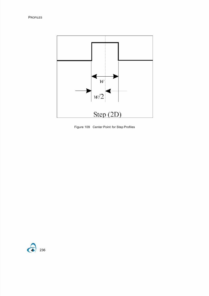
7/21/2019 OptiMode User Reference
http://slidepdf.com/reader/full/optimode-user-reference 240/339
PROFILES
236
Figure 109 Center Point for Step Profiles

7/21/2019 OptiMode User Reference
http://slidepdf.com/reader/full/optimode-user-reference 241/339
PROFILES
237
Fiber Profile
The Waveguide Depth reference point of the Fiber Profile window-frame is located inits middle. The center point of the profile is aligned with the center (core) of the fibercross-section.
Figure 110 Center Point for Fiber Profiles

7/21/2019 OptiMode User Reference
http://slidepdf.com/reader/full/optimode-user-reference 242/339
PROFILES
238
Diffused and User Defined Profiles
The Waveguide Depth reference point of the Diffused and User Defined Profile islocated at the Profile surface (top) level. The waveguide "body" is always locatedbelow the Waveguide Depth, or the Profile surface level.
Figure 111 Center poin t for Diffused and Function Defined Profil es
Waveguide profiles allow the manipulation of waveguides in the Y direction
independent of the wafer definition. All waveguides are associated with exactly oneprofile. Each profile knows how to represent itself in two-dimensional and three-dimensional simulations. Default translations, defined by Optiwave, are supplied forthe profiles. Waveguide profiles are used by the Simulator to help generate the indexof refraction distribution of a wafer slice at any point along the direction of propagation(the Z axis). The waveguide is used to determine the index of refraction distribution atany point along the width of a waveguide. In order to do this, the waveguide profilecontains the materials used to construct the waveguide. Waveguides will not storetheir materials directly, rather, the waveguide will store its profile. The profile will storethe waveguide material. It is the profile that determines the refractive indexdistribution within the waveguide‘s cross-section.

7/21/2019 OptiMode User Reference
http://slidepdf.com/reader/full/optimode-user-reference 243/339
M ATERIALS
239
Materials
OptiMode comes with a user-defined library of materials (material database). Eachregion in the layout will be associated with a material from this library. When asimulation is performed, the simulator will look in the library to find the appropriateoptical properties to assign to each region. The optical property used depends onwhat kind of simulation is being done. For example, if the simulation is of a 3Dwaveguide made from isotropic materials, the library element will use the refractiveindex of the material. This is a complex number; the real part represents the influenceof the material on the phase velocity. A small negative number in the imaginary partwill take into account any losses that can be expected in the transmission. A materialwith gain can be accommodated by using an imaginary part with a positive sign.
If the simulation to be performed is anisotropic mode solving, then the optical propertyneeded is the tensor relating the electric field to the electric displacement, the relative
permittivity tensor.
The tensor relates two vectors with three components, so the tensor has, in general,9 components. On the other hand, the current mode solving algorithm is sensitive to
the anisotropy in the transverse plane and the propagation axis only, so thecomponents x-z, y-z, z-x, and z-y are neglected. Therefore, the 5 complex
numbers, , , , , will specify the anisotropic nature of thematerial. By using the material database, the same layout can be simulated in severalways with varying levels of detail. The database keeps the definition of the opticalproperties which are appropriate for each case.
There are several kinds of materials: Dielectric, Electrode, Diffused, FDTD-Dispersive, FDTD-Nonlinear, and FDTD-Perfect Conductor. As the names suggest,only the first three appear in OptiBPM. In OptiFDTD, Dielectric, FDTD-Dispersive,FDTD-Nonlinear, and FDTD-Perfect Conductor are available. When the ProfileDesigner is opened by itself, only the Master List is displayed, and one can see all
available materials.
The following are the material types available for OptiMode:
• Dielectric Material (OptiBPM and OptiFDTD now share the dielectric materialdefinition)
• Electrode Materials
• Diffused Material
D ε0
ε xx
ε xy
0
ε yx
ε yy
0
0 0 ε zz
E x
E y
E z
=
ε xx
ε xy
ε yx
ε yy
ε zz

7/21/2019 OptiMode User Reference
http://slidepdf.com/reader/full/optimode-user-reference 244/339
M ATERIALS
240
• FDTD Dispersive
Dielectric Material
Usable in: OptiMode, OptiBPM, OptiFDTD.
To open the Dielectri c Materials window, in the Master list, Materials folder, rightclick on the Dielectric folder and select New.
Figure 112 Dielectric material - 2D Isotrop ic tab
2D Isotropic tab
The refractive index on this page is the refractive index used by the 2D OptiBPMsimulator and mode solver. By default this is the same as the 3D isotropic refractiveindex. However, sometimes the 2D OptiBPM simulation is to use an effective indexinstead of a real (physical) index. If a different refractive index should be required inthe 2D context, unselect the Use default checkbox and enter a new refractive indexin the field.
Refractive Index: Refractive Index of the material.
Use default: When checked, set refractive index to that of the Isotropic value. Editingof the refractive index value is not allowed.

7/21/2019 OptiMode User Reference
http://slidepdf.com/reader/full/optimode-user-reference 245/339
M ATERIALS
241
3D Isotropic tab
Figure 113 Dielectric materials — 3D Isotrop ic tab
Refractive Index: Enter the real and imaginary part of the refractive index of thismaterial that is to be used by the 3D Isotropic OptiBPM solver and the 3D Isotropicmode solver.
Sellmeier : When checked, refractive index will come from sellmeier equations. Donot allow edit of refractive index.
Electro Optic Effects: See the OptiBPM documentation for a description of the useof this field.
Wavelength / Calculate: Use this field and button to calculate (and display) therefractive index value at the given wavelength from the sellmeier equations.
Electrostatic Permittivity tab
In 3D isotropic simulations that have electrodes with potential, OptiBPM will find thestatic electric field in the transverse plane. To determine this static field, it is necessary

7/21/2019 OptiMode User Reference
http://slidepdf.com/reader/full/optimode-user-reference 246/339
M ATERIALS
242
to define the relevant permittivity everywhere. Therefore all materials in the fieldshould have a defined static permittivity.
Figure 114 Dielectric Material - Electrostatic Permitt ivity tab
EpsXX, EpsYY: Enter the two main diagonal components for the calculation ofelectrostatic field in the transverse (X, Y) plane.
3D Anisotropic tab
The anisotropic mode solving algorithm is sensitive to the anisotropy in the transverseplane and the propagation axis only, so the components xz, yz, zx, and zy areneglected. Therefore, the 5 complex numbers xx, xy, yx, yy, zz will specify theanisotropic nature of the material.
The relative electric permittivity profile will, in general, be described by the complextensor of the form:
ε x y,( )
ε xx ε xy 0
ε yx
ε yy
0
0 0 ε zz
=

7/21/2019 OptiMode User Reference
http://slidepdf.com/reader/full/optimode-user-reference 247/339
M ATERIALS
243
Figure 115 Dielectric materials (Ordinary)—3D AnIsotropic tab
Use default: When checked, the diagonal terms of the permittivity tensor are filled
with square of the 3D isotropic refractive index. The off-diagonal terms are set to zero.Sellmeier will become unchecked. Editing of refractive index will not be allowed.
Sellmeier: When checked, refractive index will come from sellmeier equations. UseDefault will become unchecked. Editing of refractive index will not be allowed.
Note: Editing of refractive index is allowed when neither of the above options arechecked.
Iso Sellmeier tab
The refractive index of the material will be determined according to the formula in thedialog box.

7/21/2019 OptiMode User Reference
http://slidepdf.com/reader/full/optimode-user-reference 248/339
M ATERIALS
244
Figure 116 Isotrop ic Sellmeier tab
Wavelength: The numerical value for refractive index displayed in the 3D Isotropictab will use the formula with the number in this field as the wavelength.
M : This is the desired number of terms in the Sellmeier equation.
: This is the permittivity in the short wavelength limit.
: Enter numerical values in these columns for and in theSellmeier formula.
RI Viewer: Click here to see a plot of the refractive index vs. wavelength.
ε0
A λ Γ, , Ai λ
i, Γi

7/21/2019 OptiMode User Reference
http://slidepdf.com/reader/full/optimode-user-reference 249/339
M ATERIALS
245
Figure 117 Refractive Index-Wavelength Relationsh ip Dialog box
A range of wavelengths can be entered from start to end. To update the graph clickthe Apply button. If the Refractive Index is complex both Real and Imaginary partsmay be chosen. If it is anisotropic, use the combo box in the bottom left to choose thecomponents epsXX, epsYY, epsXY, epsYX, or epsZZ.
AnIso Sellmeier tab
Define the AnIsotropic Sellmeier equation term values with this page.

7/21/2019 OptiMode User Reference
http://slidepdf.com/reader/full/optimode-user-reference 250/339
M ATERIALS
246
Figure 118 AnIsotropic Sellmeier tab
See the section Iso Sellmeier tab above for common field definitions.
EpsXX,EpsYY... Combo: Use to choose the component the equation values are for.
Diffused Material
Usable in: OptiMode, OptiBPM.
To open the Diffused Materials window, in the Master list, Materials folder, right clickthe Diffused folder and select New.

7/21/2019 OptiMode User Reference
http://slidepdf.com/reader/full/optimode-user-reference 251/339
M ATERIALS
247
Figure 119 Diffused material
Crystal Name: Name of the host crystal.
Default: Select to make the default material.
Refractive Index: Ordinary and extraordinary refractive index of the host crystal. The Auto value of the refractive index is computed using the Sellmeier equations.
Ordinary :
Extraordinary :
where wavelength is in .
Electro optic coefficients
There are four electro optic coefiicients: r 33, r 51, r 13 and r 22. Select Default to set theelectro optic coefficients to their default values.
no
no0( )( )2
4.9048 0.11768
0.0475 λ2
–
---------------------------- – 0.027169 – =
ne
n 0( )e
4.582 0.099169
0.044432 λ2
–
---------------------------------- – 0.02915λ2
– =
λ μm
10 12 –
m V ⁄ [ ]

7/21/2019 OptiMode User Reference
http://slidepdf.com/reader/full/optimode-user-reference 252/339
M ATERIALS
248
Permittivities
Epszz and Epsxx: Low frequency permittivity‘s used for electric field calculations. Thepermittivities are LiNb03 values (default).
Wavelength: Vacuum wavelength in microns. This data can be changed in the editbox.
Crystal Cut: Refers to the crystal coordinate system, where typically, the Z-axis is theoptical axis.
Propagation direction (2D): Propagation direction can be measured in X, Y, or Zdirection.
Polarization: Refers to the wafer system, where the transverse electrical or magneticfield is parallel to the crystal surface and the crystal surface is parallel to the layoutscreen.
FDTD-Dispersive
Usable in: OptiMode, OptiFDTD.
For dispersion, the simulator calculates the complex refractive index values as afunction of wavelength. These are the available dispersion models:
• Lorentz Dispersive
• Drude Dispersive
• Lorentz-Drude Dispersive
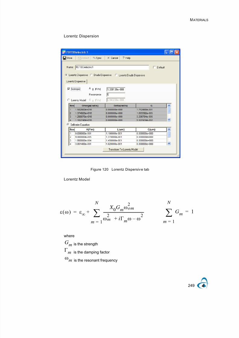
7/21/2019 OptiMode User Reference
http://slidepdf.com/reader/full/optimode-user-reference 253/339
M ATERIALS
249
Lorentz Dispersion
Figure 120 Lorentz Dispersive tab
Lorentz Model
where
is the strength
is the damping factor
is the resonant frequency
ε ω( ) ε∞
X 0Gm
ω2om
ω2m iΓ
mω ω
2 – +
--------------------------------------------
m 1=
N
∑+= Gm
m 1=
N
∑ 1=
Gm
Γm
ωm

7/21/2019 OptiMode User Reference
http://slidepdf.com/reader/full/optimode-user-reference 254/339
M ATERIALS
250
The OptiFDTD simulator can handle the materials which have a Lorentz modelresonant wavelength equal to the exciting field‘s wavelength. However the ModeSolver may not be able to find the correct mode because the calculated refractiveindex from Lorentz equation may go to infinity. An alternative is to use the Gaussianbeam as the input.
Converting the =Sellmeier equation‘ to =Lorentz Model‘
Lorentz equation
;
Input parameters (symbol) Unit Name
F/m Permittivity at zero frequency.
F/m permittivity at infinite frequency.
- Strength.
Hz Resonance frequency.
Hz Damping factor.
ε ω( ) ε∞
X 0Gm
ω2om
ω2m iΓmω ω
2 – +
--------------------------------------------
m 1=
N
∑+= Gm
m 1=
N
∑ 1=
ε∞
X 0Gm
λ2
λ2
jΓmλ
2m
2πc-----------------
⎝ ⎠⎜ ⎟⎛ ⎞
λ λ2m – +
---------------------------------------------------------
m 1=
N
∑+= Γm 2δm=
ε0
ε∞
Gm
ωom
Γm

7/21/2019 OptiMode User Reference
http://slidepdf.com/reader/full/optimode-user-reference 255/339
M ATERIALS
251
Sellmeier equation
;
Input parameters (symbol) Unit Name
F/m Permitt ivity at infinite frequency.
um Resonant wavelength.
F/m Permitt ivity at resonant frequency.
um Damping factor.
ε λ( ) ε∞ Amλ
2
λ2
jΓλmλ λ
m
2 – +
--------------------------------------------
m 1=
N
∑+= A0 ε∞=
A0
λm
Am
Γλm

7/21/2019 OptiMode User Reference
http://slidepdf.com/reader/full/optimode-user-reference 256/339
M ATERIALS
252
Relation between the two models
You may enter the number of resonances in the Resonance box and enter thecoefficients for those resonances in the grid below. These boxes can be edited.OptiFDTD uses only the Lorentz model during simulation. If the Sellmeier coefficientsare entered, they will automatically be transformed to Lorentz coefficients. To see theeffect of this transformation, you may click the .Transform to Lorentz Model. button.
The grid above .Sellmeier Equation. will be populated with the converted Lorentzmodel parameters.
Select the Lorentz Model radio button to enter coefficients for the Lorentz
Dispersive model.
Drude Dispersion
Materials with Drude dispersion are optically linear materials for which the angular
frequency dependence of the dielectric permittivity can be described by the DrudeDispersion relation:
Am χ0Gm= Gm Am
χ0------=
→ → δ πcΓλm
λm
2---------------=
Γmλm
2
2πc------------ Γλm= Γm 2δ 2πcΓλm
λm
2------------------= =
χ0 Am
m 1=
N
∑=
Gm
m 1=
N
∑ 1 Am
χ0
------
m 1=
N
∑→ 1 χ0→ → ε0 ε∞ ε0→ – ε∞ Am
m 1=
N
∑+= = = =
A0 ε∞=

7/21/2019 OptiMode User Reference
http://slidepdf.com/reader/full/optimode-user-reference 257/339
M ATERIALS
253
where is the plasma angular frequency, is the collision angular frequency, and
is the permittivity at infinite frequency. For example, for a cold plasma, =
1.803274183e11 rad/s, = 2.0e10 rad/s, and = 1.0.
Figure 121 Drude Dispersive tab
Lorentz-Drude Dispersion
The governing equation for Lorentz-Drude model in time domain can be expressedas:
εr ω( ) ε∞
ω p
2
iΓω ω
2
–
-----------------------+=
ω p Γ
ε∞ ω
p
Γ ε∞
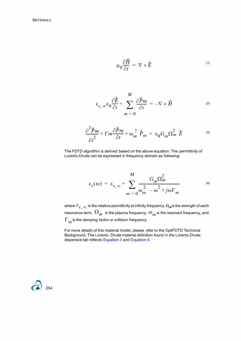
7/21/2019 OptiMode User Reference
http://slidepdf.com/reader/full/optimode-user-reference 258/339
M ATERIALS
254
The FDTD algorithm is derived based on the above equation. The permittivity ofLorentz-Drude can be expressed in frequency domain as following:
where is the relative permittivity at infinity frequency, G mis the strength of each
resonance term, is the plasma frequency, is the resonant frequency, and
is the damping factor or collision frequency.
For more details of this material model, please refer to the OptiFDTD TechnicalBackground. The Lorentz- Drude material definition found in the Lorentz-Drude
dispersive tab reflects Equation 3 and Equation 4.
(1)
(2)
(3)
(4)
μ0∂ H
∂t ------- ∇ E ×=
εr ∞, ε0
∂ E
∂t ------ ∂Pm
∂t -----------
m 0=
M
∑+ ∇ H × – =
∂2Pm
∂t 2
-------------- Γm∂Pm
∂t ----------- ω
m
2Pm+ + ε0G
mΩ
2m E =
εr ω( ) ε
r ∞,GmΩ
2m
ωm
2ω
2 – jωΓ
m+
--------------------------------------------
m 0=
M
∑+=
εr ∞,Ω
m ωm
Γm

7/21/2019 OptiMode User Reference
http://slidepdf.com/reader/full/optimode-user-reference 259/339
M ATERIALS
255
Figure 122 Lorentz-Drude Dispersive tab
Use Wavelength: Specify the Lorentz-Drude model's resonance parameters usingthe wavelength values in micrometers [µm].
Use Frequency: Use the angular frequency values in [rad/s] to specify the Lorentz-Drude model's resonance parameters. This option is selected by default.
Isotropic: Switch the Lorentz-Drude material type between isotropic and anisotropic
properties.
(F/m): Relative permittivity at infinite frequency.
Resonance: Number of resonators in Lorentz-Drude model. Please enter an integervalue.
Resonance parameters
ε∞

7/21/2019 OptiMode User Reference
http://slidepdf.com/reader/full/optimode-user-reference 260/339
M ATERIALS
256
S: Strength of the corresponding resonance term.
P: Plasma frequency/wavelength.
R: Resonant frequency/wavelength.
D: Collision frequency/wavelength.

7/21/2019 OptiMode User Reference
http://slidepdf.com/reader/full/optimode-user-reference 261/339
OPTIMODE 3D MODE SOLVER
257
OptiMode 3D Mode Solver
IntroductionIn a waveguide, a mode is one of the various possible patterns of propagatingelectromagnetic fields or standing electromagnetic fields. Each mode is characterizedby wavelength (frequency), field strength, and the electromagnetic field pattern of amode depending on the frequency, refractive indices, and waveguide geometry.
Main parts of the GUI
The 3D Mode Solver contains three main windows:
• Ref Index
• Modes found
• Output
Layout window - 3D Isotropic calculations
Displays two different graphs of the simulation:
Refractive Index: 3D view of the Refractive Index.
Figure 123 Mode Solver layout window, Refractive Index
Major component Ex: 3D view of the major component of optical electric field parallelto X.

7/21/2019 OptiMode User Reference
http://slidepdf.com/reader/full/optimode-user-reference 262/339
OPTIMODE 3D MODE SOLVER
258
Figure 124 Mode Solver Layout window, Major component Ex
Layout window—3D Anisotropic calculations
Displays seven different graphs of the simulation:
epsXX, epsXY, epsYX, epsYY, epsZZ: 3D view of the different components of thepermittivity tensors.

7/21/2019 OptiMode User Reference
http://slidepdf.com/reader/full/optimode-user-reference 263/339
OPTIMODE 3D MODE SOLVER
259
Figure 125 Mode Solver layout window—eps XX
Major component Ex: 3D view of the major component of optical electric field parallelto X.
Figure 126 Mode Solver layout window, Major component Ex
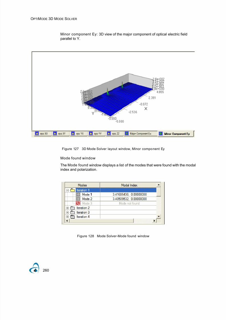
7/21/2019 OptiMode User Reference
http://slidepdf.com/reader/full/optimode-user-reference 264/339
OPTIMODE 3D MODE SOLVER
260
Minor component Ey: 3D view of the major component of optical electric fieldparallel to Y.
Figure 127 3D Mode Solver layout window, Minor component Ey
Mode found window
The Mode found window displays a list of the modes that were found with the modal
index and polarization.
Figure 128 Mode Solver-Mode found window

7/21/2019 OptiMode User Reference
http://slidepdf.com/reader/full/optimode-user-reference 265/339
OPTIMODE 3D MODE SOLVER
261
Output window
The Output window can be moved around from its original location. The Notification
tab displays the time that the calculation starts, the number of modes found, and thetime that the calculation ends. The Error tab displays any notifications or errors that
may occur in the process.
Figure 129 Mode Solver—Output window
Main menu bar
The Main menu bar contains the menus that are available in the 3D Mode Solver.Many of these menu items are also available as buttons on the toolbars.
Figure 130 Main menu bar
Toolbars
Select the toolbars that you want to have available.
Standard Available in all views. Displaysinformation about OptiModeSolver.
SolvingToolbar
Resume, pause, or abort thesimulation. Only available whenthe solver is running.

7/21/2019 OptiMode User Reference
http://slidepdf.com/reader/full/optimode-user-reference 266/339
OPTIMODE 3D MODE SOLVER
262
DataView
Select the Real, Imaginary, Amplitude, Phase, Intensity, ordB views.
Dockers Open or close the Mode foundand Output windows.
Avis / 3DGraph
Available for both the Refrac-tive Index and Major compo-nent EX views.

7/21/2019 OptiMode User Reference
http://slidepdf.com/reader/full/optimode-user-reference 267/339
OPTIMODE 3DMSIM MENUS AND BUTTONS
263
OptiMode 3DMSim menus and buttons
This section describes the menus and buttons available in the 3D Mode Solver.
File menu
View menu
File Menu Item Toolbar Button Description
Exit Closes OptiMode Solver.
Fi le Menu Item Toolbar
Button
Description
Toolbars Select the toolbars that you want to make available in the GUI.
Status Bar Select to display the Satus Bar. Displays the cursor position coordinates.
Output Window Select to display the Output Window. Displays notification and errormessages regarding the script.
3D Graph Items (Detailed in “ View menu” on page 119)
Data View
Real Displays the real part of the simulation graph.
Imaginary Displays the imaginary part of the simulation graph.
Ampl itude Displays the amplitude of the simulation graph.
Phase Displays the phase of the simulation graph.
Intensity Displays the intensity of the simulation graph.
dB Applies the dB to the simulation graphic. Available for amplitude and
intensity.

7/21/2019 OptiMode User Reference
http://slidepdf.com/reader/full/optimode-user-reference 268/339
OPTIMODE 3DMSIM MENUS AND BUTTONS
264
Solve menu
Data menu
Customize Customize the toolbars and the buttons.
Fi le Menu Item Toolbar
Button
Description
Pause Pauses the simulation.
Resume Resumes teh simulation after it has been paused.
Abor t A message appears and prompts you to verify that you want to abort the
simulation.
Data Menu Item Description
Save Refractive Index (es)... Opens the Save Refractive Index dialog box. Select the folder to save the
file to.
Save Modal Indexes... Opens the Save Modal Indices dialog box. Select the folder to save the file
to.
Save Mode(s)... Opens the Save Mode(s) dialog box. Select the directory to save the file to
and the base file name
Customize Customize the toolbars and the buttons.
Fi le Menu Item Toolbar
Button
Description

7/21/2019 OptiMode User Reference
http://slidepdf.com/reader/full/optimode-user-reference 269/339
OPTIMODE 3DMSIM MENUS AND BUTTONS
265
Preferences menu
Help menu
OptiMode Solver functions
This section contains descriptions of the functions and dialog boxes that you accessfrom OptiMode Solver 3D menus.
Note: Standard Windows functions and dialog boxes are not described.
Mode Found
The Mode Found window displays the modes that are found. The modal index andthe polarization are displayed for each mode found. If you set the 3D Mode Solver tofind more modes than the number of modes that are present, a red symbol appearsbeside the first unfound mode and the calculation stops.
Preferences Menu Item Descr ip tion
Region of Interest Select the start and end points for the Z axis and the X axis.
Height Plot Settings Select five different styles: Wireframe, Surface, Bar chart, Lines and Points.
Axis Settings Select settings for the X, Y, and Z axes.
Image Map Settings Set the image orientation, aspect ratio, and grid density.
Palette Settings Select the different settings for the palette.
Data Clamping Select the diferent settings for refractive index XZ-plane axis and the
sampling resolution.
Save settings now Saves teh setting automatically as you work.
Save settings on close Saves the settings automatically when you close OptiMode.
Layout Options Select the Grid, Layout Axes, and Zoom Method. Only available in thelayout view.
Preferences Menu Item Descr ip tion
Help Topics Provides information on OptiMode Solver.
About Opt iMode Solver. Provides information about Optiwave - mailing address, telephone and fax
numbers, e-mail address, and URL.

7/21/2019 OptiMode User Reference
http://slidepdf.com/reader/full/optimode-user-reference 270/339
OPTIMODE 3DMSIM MENUS AND BUTTONS
266
Figure 131 Mode found window—First unfound mode
A message appears in the output (error) window advising you that the mode could notbe found.
Figure 132 Output Window—Unfound Mode Notification
To save the settings, from the Data menu, select one of the following:• Save Refractive Index (es)
• Save Modal Indexes
• Save Mode(s)
7/21/2019 OptiMode User Reference
http://slidepdf.com/reader/full/optimode-user-reference 271/339
OPTIMODE 3DMSIM MENUS AND BUTTONS
267
Status Bar
To view the Status Bar, from the View menu, select Status Bar .
Figure 133 Status bar
The Status Bar indicates whether the 3D Mode Solver is searching for modes or hascompleted the search.
3D Graph Items
To view the following items in the layout, from the View menu, select 3D Graph Items,and then select the item that you want to view. A check mark appears beside theselected item. For item descriptions see “3D Graph Items” on page 132.
Customize
Open the Customize dialog box to select the settings for the OptiMode Analyzerlayout.
Toolbars tab
Select the toolbars that you want available in the layout, and create new toolbars.

7/21/2019 OptiMode User Reference
http://slidepdf.com/reader/full/optimode-user-reference 272/339
OPTIMODE 3DMSIM MENUS AND BUTTONS
268
Figure 134 Customize dialog box—Toolbars tab
Select toolbars: Click the check box beside the toolbars that you want to select.
Show Toolti ps: Displays the name of the button on a toolbar when you position the
cursor on top of the button.
Cool Look: Changes the outline appearance of the toolbar buttons. When you selectthe Cool Look check box, the button outlines disappear.
Figure 135 Select Cool Look check box - result
When you clear the Cool Look check box, button outlines appear.
Figure 136 Clear Cool Look check box - result

7/21/2019 OptiMode User Reference
http://slidepdf.com/reader/full/optimode-user-reference 273/339
OPTIMODE 3DMSIM MENUS AND BUTTONS
269
Large Buttons: Displays larger buttons.
Figure 137 Large buttons vs. Small buttons
New: To create a new toolbar, click New. The New Toolbar dialog box appears.
Figure 138 New Toolbar dialog box
Type a name for the toolbar, and click OK. The new toolbar appears in the list ofavailable toolbars.
Reset: Restores default settings.
Commands tab
Select a toolbar to view the buttons that are on the toolbar. Select a button to view abrief description of what the button does.

7/21/2019 OptiMode User Reference
http://slidepdf.com/reader/full/optimode-user-reference 274/339
OPTIMODE 3DMSIM MENUS AND BUTTONS
270
Figure 139 Customize dialog box—Commands tab
To add buttons to a new toolbar, drag the buttons that you want to use to the toolbarthat you want to add them to.
Data menu
Save Refract ive Index (es)...
To open the Save Refract ive Index dialog box, from the Data menu, select Save
Refractive Index (es). The file extension is *.rid.
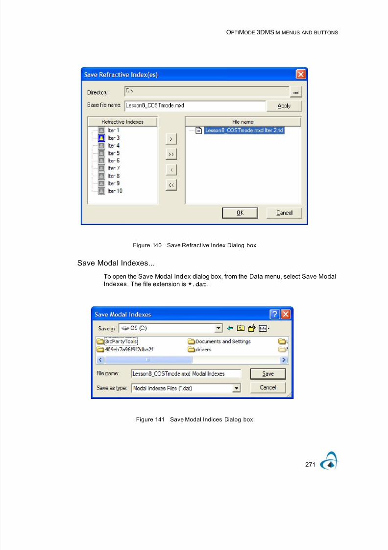
7/21/2019 OptiMode User Reference
http://slidepdf.com/reader/full/optimode-user-reference 275/339
OPTIMODE 3DMSIM MENUS AND BUTTONS
271
Figure 140 Save Refractive Index Dialog box
Save Modal Indexes...
To open the Save Modal Index dialog box, from the Data menu, select Save Modal
Indexes. The file extension is *.dat.
Figure 141 Save Modal Indices Dialog box
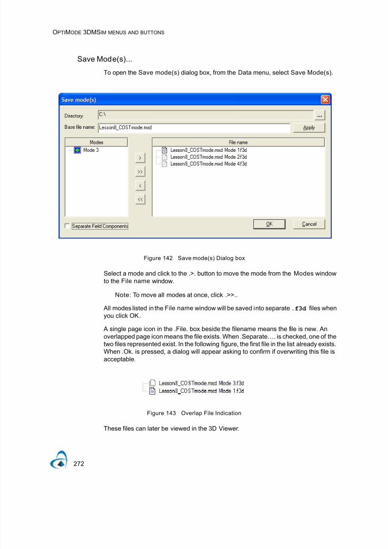
7/21/2019 OptiMode User Reference
http://slidepdf.com/reader/full/optimode-user-reference 276/339
OPTIMODE 3DMSIM MENUS AND BUTTONS
272
Save Mode(s)...
To open the Save mode(s) dialog box, from the Data menu, select Save Mode(s).
Figure 142 Save mode(s) Dialog box
Select a mode and click to the .>. button to move the mode from the Modes windowto the File name window.
Note: To move all modes at once, click .>>..
All modes listed in the File name window will be saved into separate .f3d files whenyou click OK.
A single page icon in the .File. box beside the filename means the file is new. Anoverlapped page icon means the file exists. When .Separate…. is checked, one of thetwo files represented exist. In the following figure, the first file in the list already exists.When .Ok. is pressed, a dialog will appear asking to confirm if overwriting this file isacceptable.
Figure 143 Overlap File Indication
These files can later be viewed in the 3D Viewer.

7/21/2019 OptiMode User Reference
http://slidepdf.com/reader/full/optimode-user-reference 277/339
OPTIMODE 3DMSIM MENUS AND BUTTONS
273
Figure 144 3D Viewer
Separate Field Components: Use this check box to save full vector results inseparate ..f3d. files. When selected, the filenames box will show entries with(depending on the mode polarization) information of the form .Major_Ex/Minor_Ey.appended. This means when .Ok. is pressed, two files will be produced for everymode chosen.

7/21/2019 OptiMode User Reference
http://slidepdf.com/reader/full/optimode-user-reference 278/339
OPTIMODE 3DMSIM MENUS AND BUTTONS
274
Figure 145 Save mode(s) Seperately Dialog settings
Iterated Results
When a script has been used to generate solve results, the mode save dialog willresemble the next figure.

7/21/2019 OptiMode User Reference
http://slidepdf.com/reader/full/optimode-user-reference 279/339
OPTIMODE 3DMSIM MENUS AND BUTTONS
275
Figure 146 Save mode(s) With Iteration Dialog box
Notice that filenames now include the iteration number in the format. Otherwise, usingthe dialog is the same as without iterations.
3D Graph Settings
See the section “3D Graph Settings” on page 148 for details.

7/21/2019 OptiMode User Reference
http://slidepdf.com/reader/full/optimode-user-reference 280/339
OPTIMODE 3DMSIM MENUS AND BUTTONS
276

7/21/2019 OptiMode User Reference
http://slidepdf.com/reader/full/optimode-user-reference 281/339
OPTIMODE ANALYZER
277
OptiMode Analyzer
After you run a simulation, view the results in OptiMode Analyzer.
Figure 147 OptiMode Analyzer Window
Main parts of the GUI
The OptiMode_Analyzer GUI contains the following main windows:
• Analysis Tools• Layout
• Output

7/21/2019 OptiMode User Reference
http://slidepdf.com/reader/full/optimode-user-reference 282/339
OPTIMODE ANALYZER
278
Analysis Tools
The Navigator window displays the types of views that are available for a giveniteration.
Figure 148 Navigator Window

7/21/2019 OptiMode User Reference
http://slidepdf.com/reader/full/optimode-user-reference 283/339
OPTIMODE ANALYZER
279
Layout Window
The Layout window displays the graph, iteration, notes, etc that you selected in theNavigator window.
Figure 149 Layout Window - Refractive Index View
Figure 150 Layout Window - Modal Result View

7/21/2019 OptiMode User Reference
http://slidepdf.com/reader/full/optimode-user-reference 284/339
OPTIMODE ANALYZER
280
Figure 151 Layout Window - Notes
Figure 152 Layout Window - Solver Information

7/21/2019 OptiMode User Reference
http://slidepdf.com/reader/full/optimode-user-reference 285/339
OPTIMODE ANALYZER
281
Figure 153 Layout Window - Modal Index (optional)
Figure 154 Layout Window - Group Delay (optional)

7/21/2019 OptiMode User Reference
http://slidepdf.com/reader/full/optimode-user-reference 286/339
OPTIMODE ANALYZER
282
Figure 155 Layout Window - Dispersion (optional)
Output window
The Output window can be moved around from its original location. The Notification
and Error tabs are there as tools to display any notifications or errors that may occurin the process. The Error tab is only for layout objects.
Main menu bar
The main menu bar contains the menus that are available in OptiMode Analyzer.Many of these menu items are also available as buttons on the toolbars.
Figure 156 Main menu bar
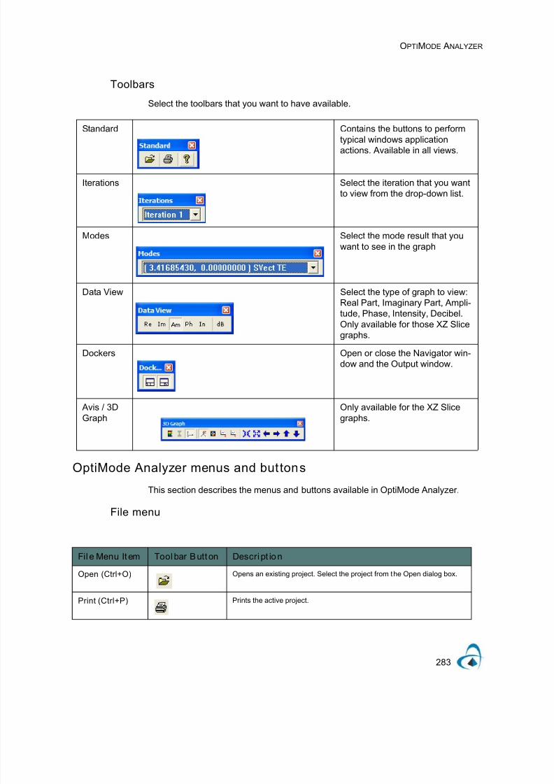
7/21/2019 OptiMode User Reference
http://slidepdf.com/reader/full/optimode-user-reference 287/339
OPTIMODE ANALYZER
283
Toolbars
Select the toolbars that you want to have available.
OptiMode Analyzer menus and buttons
This section describes the menus and buttons available in OptiMode Analyzer.
File menu
Standard Contains the buttons to perform
typical windows applicationactions. Available in all views.
Iterations Select the iteration that you wantto view from the drop-down list.
Modes Select the mode result that youwant to see in the graph
Data View Select the type of graph to view:Real Part, Imaginary Part, Ampli-tude, Phase, Intensity, Decibel.Only available for those XZ Slicegraphs.
Dockers Open or close the Navigator win-dow and the Output window.
Avis / 3DGraph Only available for the XZ Slicegraphs.
Fil e Menu It em Toolbar Button Descript ion
Open (Ctrl+O) Opens an existing project. Select the project from the Open dialog box.
Print (Ctrl+P) Prints the active project.

7/21/2019 OptiMode User Reference
http://slidepdf.com/reader/full/optimode-user-reference 288/339
OPTIMODE ANALYZER
284
Print Setup Allows you to set up the printer, page size, orientation, and allows you to
set other printing option.
Recent files Lists the most recent files that you worked on.
Exit Closes OptiMode Analyzer.
Fil e Menu It em Toolbar Button Descript ion

7/21/2019 OptiMode User Reference
http://slidepdf.com/reader/full/optimode-user-reference 289/339
OPTIMODE ANALYZER
285
View Menu
View Menu
Item
Toolbar Button Descr ipt ion
Toolbars Select the toolbars that you want to make available in the GUI.
Navigator Select to open or close the Navigator window. Displays the types of viewsavailable in OptiMode Analyzer.
Status Bar Select to display the Status Bar.
Output Window Select to display the Output Window. Displays notification and errormessages regarding the script.
3D Graph Items (Detailed in “View menu” on page 119)
Data View
Real Displays the Real Refractive Index data view in the Anal yzer graph.
Imaginary Displays the Imaginary Refractive Index data view in the Analyzer graph.
Amp li tude Displays the Ampl itude vs Distance data view in the Analyzer graph.
Phase Displays the Phase vs Distance data view in the Analyzer graph.
Intensity Displays the Intensity vs Distance data view in the Analyzer graph.
dB Displays the Decibel vs Distance data view in the Analyzer graph.
Iteration Select the iteration that you want to view in the layout window.
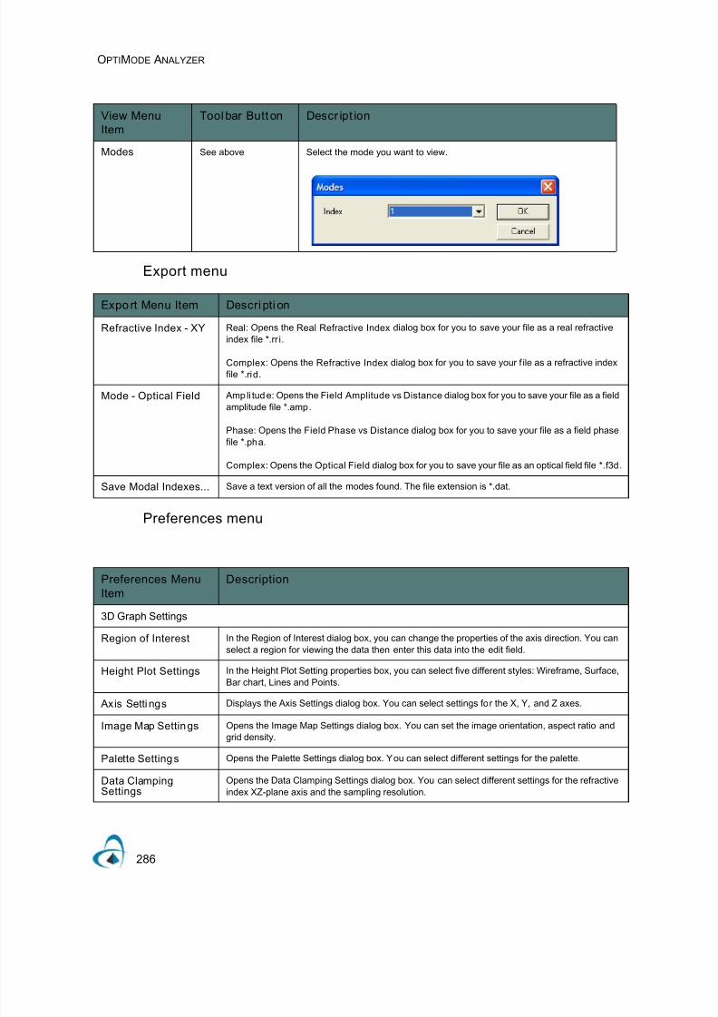
7/21/2019 OptiMode User Reference
http://slidepdf.com/reader/full/optimode-user-reference 290/339
OPTIMODE ANALYZER
286
Export menu
Preferences menu
Modes See above Select the mode you want to view.
Expo rt Menu Item Descripti on
Refractive Index - XY Real: Opens the Real Refractive Index dialog box for you to save your file as a real refractive
index file *.rr i.
Complex: Opens the Refractive Index dialog box for you to save your f ile as a refractive index
file *.rid.
Mode - Optical Field Amp li tude: Opens the Field Amplitude vs Distance dialog box for you to save your file as a field
amplitude file *.amp .
Phase: Opens the Field Phase vs Distance dialog box for you to save your file as a field phase
file *.pha.
Complex: Opens the Optical Field dialog box for you to save your file as an optical field file *.f3d.
Save Modal Indexes... Save a text version of all the modes found. The file extension is *.dat.
Preferences Menu
Item
Description
3D Graph Settings
Region of Interest In the Region of Interest dialog box, you can change the properties of the axis direction. You can
select a region for viewing the data then enter this data into the edit field.
Height Plot Settings In the Height Plot Setting properties box, you can select five different styles: Wireframe, Surface,
Bar chart, Lines and Points.
Axis Setti ngs Displays the Axis Settings dialog box. You can select settings for the X, Y, and Z axes.
Image Map Settings Opens the Image Map Settings dialog box. You can set the image orientation, aspect ratio andgrid density.
Palette Settings Opens the Palette Settings dialog box. You can select different settings for the palette.
Data ClampingSettings
Opens the Data Clamping Settings dialog box. You can select different settings for the refractive
index XZ-plane axis and the sampling resolution.
View Menu
Item
Toolbar Button Descr ipt ion

7/21/2019 OptiMode User Reference
http://slidepdf.com/reader/full/optimode-user-reference 291/339
OPTIMODE ANALYZER
287
Help menu
Save setting now Default setting. Saves the settings automatically as you work.
Save settings on close Saves the settings automatically when you close OptiMode.
Help Menu It em Toolbar Button Descr ipt ion
Help Topics Provides information on OptiMode.
About Opt iMode Analyzer
Provides information about Optiwave - mailing address, telephone and fax
numbers, e-mail address, and URL.
Preferences Menu
Item
Description
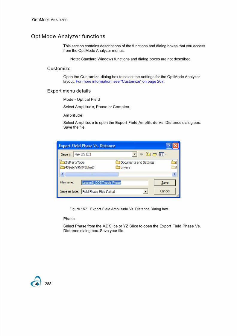
7/21/2019 OptiMode User Reference
http://slidepdf.com/reader/full/optimode-user-reference 292/339
OPTIMODE ANALYZER
288
OptiMode Analyzer functions
This section contains descriptions of the functions and dialog boxes that you accessfrom the OptiMode Analyzer menus.
Note: Standard Windows functions and dialog boxes are not described.
Customize
Open the Customize dialog box to select the settings for the OptiMode Analyzerlayout. For more information, see “Customize” on page 267.
Export menu details
Mode - Optical Field
Select Ampl itude, Phase or Complex.
Ampl itude
Select Ampl itude to open the Export Field Amplitude Vs. Distance dialog box.Save the file.
Figure 157 Export Field Ampli tude Vs. Distance Dialog box
Phase
Select Phase from the XZ Slice or YZ Slice to open the Export Field Phase Vs.
Distance dialog box. Save your file.

7/21/2019 OptiMode User Reference
http://slidepdf.com/reader/full/optimode-user-reference 293/339
OPTIMODE ANALYZER
289
Figure 158 Export Field Phase Vs. Distance Dialog box
Complex
Select Complex to open the Export Optical Field dialog box. Save the file.
Figure 159 Export Optical Field
Refractive Index
Select Real or Complex.
RealSelect Real to open the Export Real Refractive Index dialog box. Save the file.

7/21/2019 OptiMode User Reference
http://slidepdf.com/reader/full/optimode-user-reference 294/339
OPTIMODE ANALYZER
290
Figure 160 Export Real Refractive Index
Complex
Select Complex to open the Export Refractive Index dialog box. Save the file.
Figure 161 Export Refractive Index
Preferences menu details
For more information, see “Preferences menu” on page 286.

7/21/2019 OptiMode User Reference
http://slidepdf.com/reader/full/optimode-user-reference 295/339
APPENDIX A: OPTI2D GRAPH CONTROL
291
Appendix A: Opti2D Graph Control
The Graph control is a versatile, powerful easy-to-use tool for observing data. Thissection gives a brief description of some of the 2D graph control features and anexplanation of how to use them.
Figure 162 Opti2D Graph Contro l

7/21/2019 OptiMode User Reference
http://slidepdf.com/reader/full/optimode-user-reference 296/339
APPENDIX A: OPTI2D GRAPH CONTROL
292
User interface features
Information windowsThere are two main windows visible on the main display:
• Info-window
• Legend-window
Both can be launched using the Graph menu or Graph tools.
Feature Description
Large data handling capabilities Opti2d Graph control is capable of handling millions of points.
Optimized drawing Even with a large number of data points, Opti2D Graph Control is opt imized to al low forsmooth tracing and planning of graphs.
Moveable information windows Moveable information windows allos for placement of the windows in the most
convenient location in the graph window.
Crosshair Visible cross to make seeing trace points easier.
Graph toolbox The popup Graph toolbox allows easier access to the view/organizing/editing
capabilities of the Opti2D Graph tool.
Graph Menu button The Graph menu button allows you to access a full list of functionality associated with
the graphs and their data.

7/21/2019 OptiMode User Reference
http://slidepdf.com/reader/full/optimode-user-reference 297/339
APPENDIX A: OPTI2D GRAPH CONTROL
293
Info-window
Figure 163 Info-Window
When you access the Info-window, it displays in the work area of the graph view. Bydefault, it displays the current position (in data-base coordinates) of the cursor. Whenyou add marker, tracers, and regions, the Info-Window expands to show the details ofthese components.
When you use the Select tool, if you double click in the window, the Info-Windowproperties dialog displays (see Figure 164).
Figure 164 Info-Window settings dialog box

7/21/2019 OptiMode User Reference
http://slidepdf.com/reader/full/optimode-user-reference 298/339
APPENDIX A: OPTI2D GRAPH CONTROL
294
Legend
You can switch the Legend on and off using the Legend tool in the Graph toolbox, orthe Graph menu. The Legend displays a list of all the curves displayed in the graphwith the corresponding line color that is used to display those curves. Use the
Minimize/Maximize button to change the display of the Legend, or close the Legendby using the Close button.
Figure 165 Legend
Graph toolbox
To access the Graph toolbox, right-click in the graph view. Most graphediting/viewing/organizing capabilities are accessible using the toolbox (see Figure166).
Figure 166 Popup Graph Toolbox

7/21/2019 OptiMode User Reference
http://slidepdf.com/reader/full/optimode-user-reference 299/339
APPENDIX A: OPTI2D GRAPH CONTROL
295
Graph tools
Graph menu
item
Toolbar button Descript ion
Select Allows you to manipulate and move most of the objects on the Graph.
Note: To edit the properti es of an object, double-click the object in the
graph view.
Zoom Zoom in: You can select a rectangular region, or click in the graph view for
proportional zoom in.
Extra features:
•Zoom out: Hold Ctrl and click to perform a zoom out.
•Reset Zoom Level: Double-click in the graph view to return to the default
Zoom level.
Pan Allows you to pan from side to side in the graph display to see parts of the graph
that may not be visible at the existing Zoom level or resolution.
To Pan, click to grab the display, and move teh cursor from side to side.
Extra features:
•If you press Ctrl while panning the graph display, accelerated pan is engaged,
which makes the pan much faster. This feature is useful when you work under a
high zoom factor.
Grid Allows you to turn the grid lines on/off. Click on the grid tool to toggle the grid
lines.
Tracer Allows you to select a curve and trace over it while viewing the exact positional
values on the curve in the Info Winodw. To select a different curve, double clickin the graph view.
Extra features:
•You can freeze the tracer by pressing Ctrl. Click to place a marker on the curveat that position.
•Press Shift and drag the cursor to put the tracer into a high-resolution trace thatiterates through each element in the source data array. This allows for a verydetailed scan of the data and to find peaks that the standard trace may omit.
Trace Allows you to select a curve and trace over it while viewing the exact positional
values on the curve in the Info Window. The Difference Tracer differs from the
Tracer tool because it allows you to create a second tracer to compare values on
either the same curve or on different curves. To select the next curve, double clickon the curve in the graph view.
Extra features:
•By Pressing the Control Key the tracer will freeze in its present position. Then bypressing the left mouse button a marker will be placed on that position on thecurve.
•By Pressing the shift key and dragging the mouse the tracer jumps into a highresolution trace that iterates through each element in the source data array. Thisallows for a very detailed scan of the data and to find peaks that the standardtrace may omit.
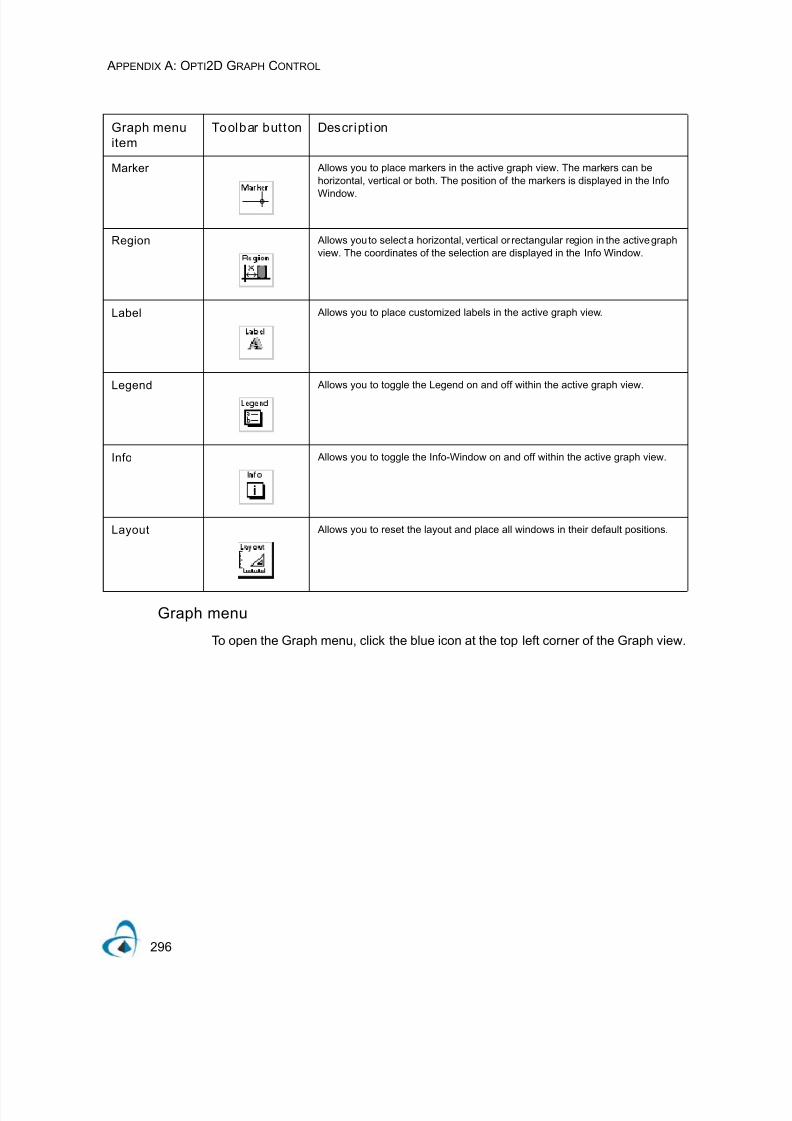
7/21/2019 OptiMode User Reference
http://slidepdf.com/reader/full/optimode-user-reference 300/339
APPENDIX A: OPTI2D GRAPH CONTROL
296
Graph menu
To open the Graph menu, click the blue icon at the top left corner of the Graph view.
Marker Allows you to place markers in the active graph view. The markers can be
horizontal, vertical or both. The position of the markers is displayed in the Info
Window.
Region Allows you to select a horizontal, vertical or rectangular region in the active graphview. The coordinates of the selection are displayed in the Info Window.
Label Allows you to place customized labels in the active graph view.
Legend Allows you to toggle the Legend on and off within the active graph view.
Info Allows you to toggle the Info-Window on and off within the active graph view.
Layout Allows you to reset the layout and place all windows in their default positions.
Graph menu
item
Toolbar button Descript ion

7/21/2019 OptiMode User Reference
http://slidepdf.com/reader/full/optimode-user-reference 301/339
APPENDIX A: OPTI2D GRAPH CONTROL
297
Figure 167 Graph Menu
Graph Menu button
The Graph Menu button is in the top left corner of the graph view.
Tools
The tools available from the Graph menu include:
• Select
• Zoom• Pan
• Grid
• Tracer
• Difference Tracer
• Marker

7/21/2019 OptiMode User Reference
http://slidepdf.com/reader/full/optimode-user-reference 302/339
APPENDIX A: OPTI2D GRAPH CONTROL
298
• Region
• Label
Windows
The information windows available in the Graph Menu include:
• Legend
• Info Window
• Reset Layout
Printing and exporting files
Opens the Print dialog box and allows you to print an image of the active graph view.
Figure 168 Print Dialog box
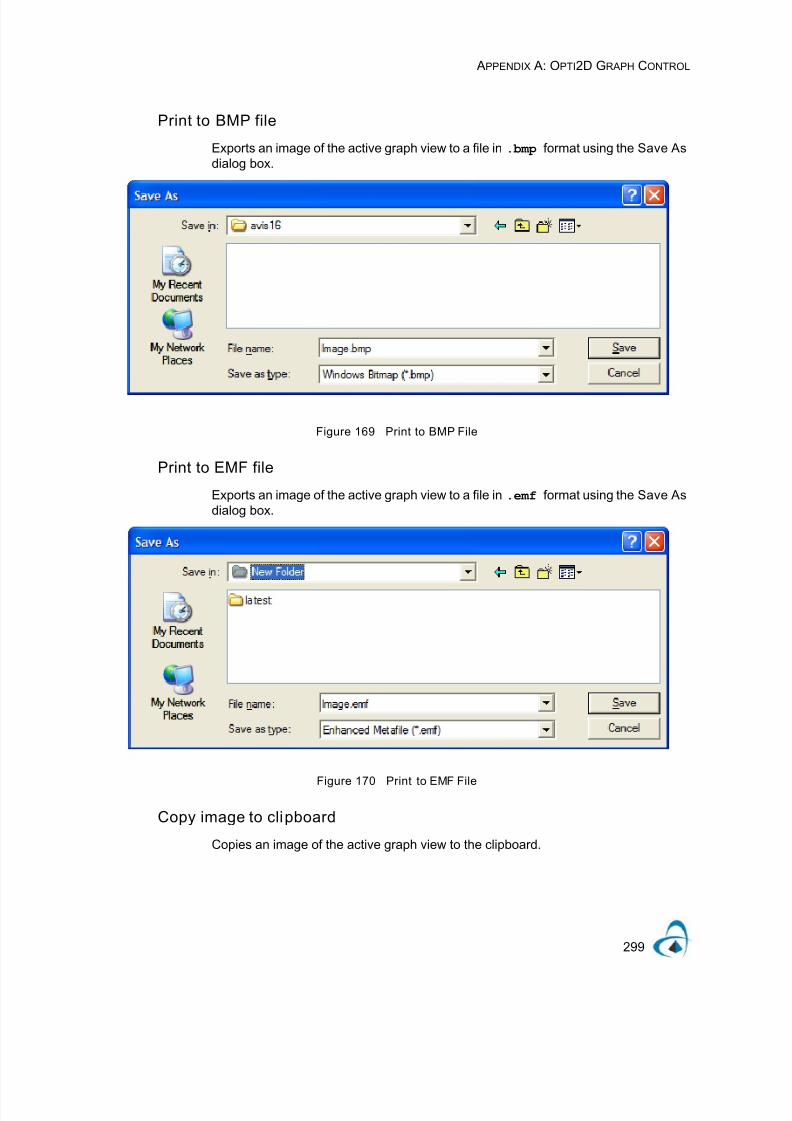
7/21/2019 OptiMode User Reference
http://slidepdf.com/reader/full/optimode-user-reference 303/339
APPENDIX A: OPTI2D GRAPH CONTROL
299
Print to BMP file
Exports an image of the active graph view to a file in .bmp format using the Save As
dialog box.
Figure 169 Print to BMP File
Print to EMF file
Exports an image of the active graph view to a file in .emf format using the Save As
dialog box.
Figure 170 Print to EMF File
Copy image to clipboard
Copies an image of the active graph view to the clipboard.

7/21/2019 OptiMode User Reference
http://slidepdf.com/reader/full/optimode-user-reference 304/339
APPENDIX A: OPTI2D GRAPH CONTROL
300
Utilities
Tool setup: Allows you to modify the properties of some of the tools.
Note: The tool property dialog only launches if the active tool allows settings to
be changed.
Set Active Display: Allows you to select the active display. For more information see“Displays” on page 301.
Properties: Allows you to launch the Graph Properties dialog. For more informationsee “Graph Properties dialog” on page 302.
Export Data...: Launches a dialog box that displays a list of all the curves on thegraph control and displays the data coordinates of those curves. It also allows you toexport the data points to a text file.
Figure 171 Data Table dialog box
Help
Launches a help dialog box specifically related to the Opti2D Graph Control.
Import Curve: Allows you to import a curve from a text file. The file must be in theformat below.
X1 (tab) Y1
X2 (tab) Y2
Etc…

7/21/2019 OptiMode User Reference
http://slidepdf.com/reader/full/optimode-user-reference 305/339
APPENDIX A: OPTI2D GRAPH CONTROL
301
Ex:
// (Beginning of file) (this line should not be in the file)
123.23 123.45
123.24 124.55
123.25 555.5123.26 222.22
//(End of file) (this line should not be in the file)
Displays
The graph is made up of layered displays. Each display has a pair of axes. By default,the control contains one display with Axis X on the bottom of the display and Axis Yon the left. In the case of complex graphs that require more than one pair of axes,more than one display exists.
Figure 172 Active Display Dialog box
Any objects that you place on the graph are placed on the active graph view.Therefore, if you place a marker on the graph and Display 1 is active, the new marker
is based on the coordinate system of Display 1. If you want to add a marker on Display2, you must select the main menu in the Graph menu. This launches the GraphDisplay dialog, which permits you to select a different display. In complex graphs, thedisplays are layered one on top of the other.
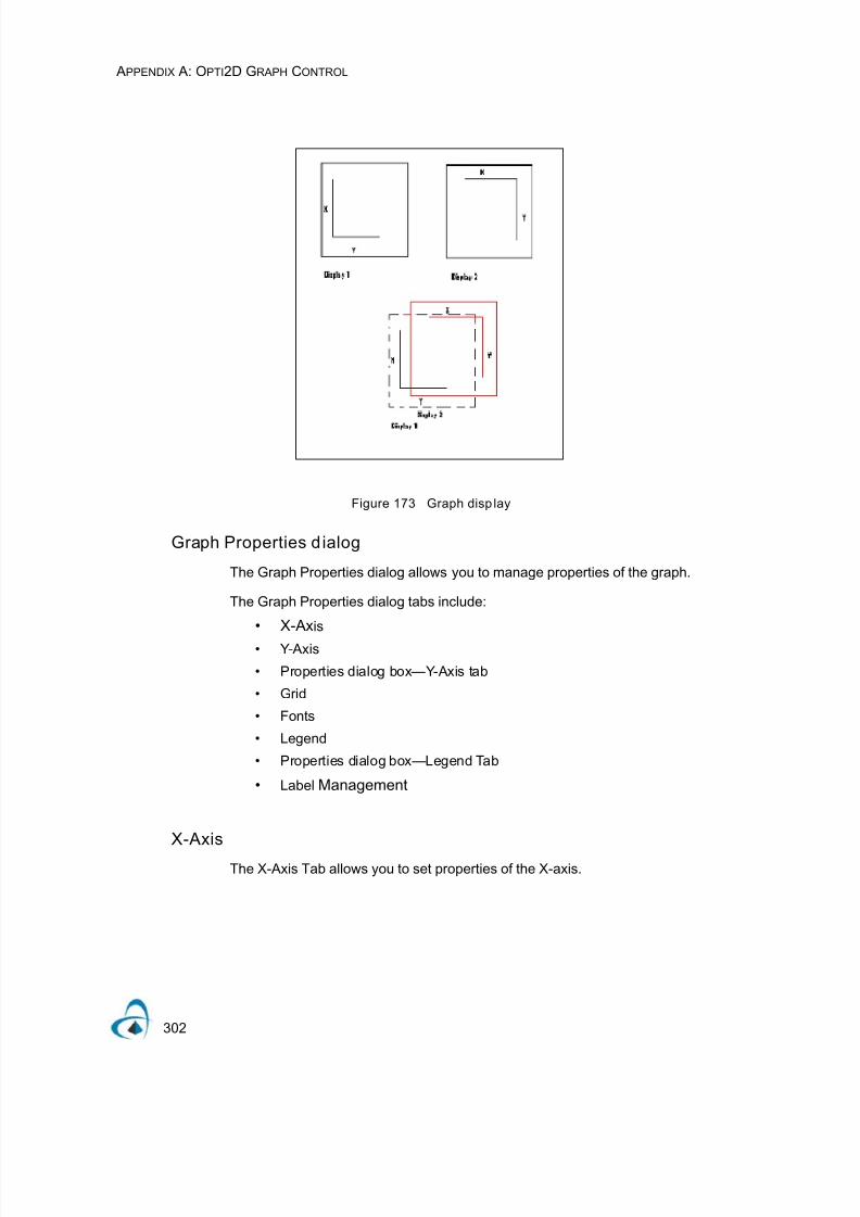
7/21/2019 OptiMode User Reference
http://slidepdf.com/reader/full/optimode-user-reference 306/339
APPENDIX A: OPTI2D GRAPH CONTROL
302
Figure 173 Graph disp lay
Graph Properties d ialog
The Graph Properties dialog allows you to manage properties of the graph.
The Graph Properties dialog tabs include:
• X-Axis
• Y-Axis
• Properties dialog box—Y-Axis tab
• Grid
• Fonts
• Legend
• Properties dialog box—Legend Tab
• Label Management
X-Axis
The X-Axis Tab allows you to set properties of the X-axis.

7/21/2019 OptiMode User Reference
http://slidepdf.com/reader/full/optimode-user-reference 307/339
APPENDIX A: OPTI2D GRAPH CONTROL
303
Figure 174 Properties Dialog box - X-Axis tab
The values in Scale Type can be:
• Linear
• Logarithmic
• DB
The values in Format Value can be:
• Decimal: simple decimal values (1000.0, 2000.0, 3000.0)
• Exponential: exponential notation (1.0-e3, 2.0-e3, 3.0-e3)
• Engineering: engineering notation (1k, 2k, 3k)
• Scientific: scientific notation (1.0 x 103,2.0 x 103, 3.0 x 10³)
Prefix: You can place a prefix string before each of the scale values.
Suffix: You can place a suffix string after each of the scale values (e.g. 1000.0 nm )
Au tomat ic Range, Min Value, Max Value: You can check Automatic Range, whichsets the range according to the curves in the displays, or force the axis range tocertain values.
Tick marks: You can set the number of major and minor tick marks on the Axis.
Y-Axis
The Y-Axis Tab allows you to set properties of the Y-axis. To see descriptions of theY-Axis dialog fields, see .X-Axis. above.
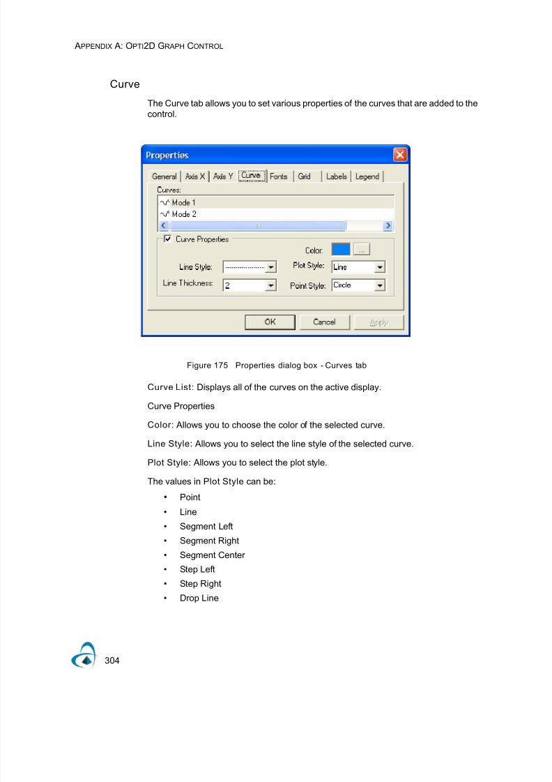
7/21/2019 OptiMode User Reference
http://slidepdf.com/reader/full/optimode-user-reference 308/339
APPENDIX A: OPTI2D GRAPH CONTROL
304
Curve
The Curve tab allows you to set various properties of the curves that are added to thecontrol.
Figure 175 Properties dialog box - Curves tab
Curve List: Displays all of the curves on the active display.
Curve PropertiesColor: Allows you to choose the color of the selected curve.
Line Style: Allows you to select the line style of the selected curve.
Plot Style: Allows you to select the plot style.
The values in Plot Style can be:
• Point
• Line
• Segment Left
• Segment Right
• Segment Center
• Step Left
• Step Right
• Drop Line

7/21/2019 OptiMode User Reference
http://slidepdf.com/reader/full/optimode-user-reference 309/339
APPENDIX A: OPTI2D GRAPH CONTROL
305
Line Thickness: Allows you to select the thickness of the currently plotted curve line.
Values range from 1 to 8.
Point Style: Allows you to select the style in which each point on the curve will be
drawn.The values in Point Style can be:
• None
• Circle
• Square
• Diamond
• Cross
• X
• Triangle
• Star
Grid
The Grid tab allows you to select which of the grid lines on the display are visible, andwhat color they are to be displayed in.
Figure 176 Properties Dialog box - Grid tab

7/21/2019 OptiMode User Reference
http://slidepdf.com/reader/full/optimode-user-reference 310/339
APPENDIX A: OPTI2D GRAPH CONTROL
306
Fonts
The Font Tab allows you to select the fonts used for displaying titles and axis values.
Figure 177 Properties Dialog box - Fonts tab
Legend
Legend tab simply has a toggle for the Legend Visible/Invisible.
Figure 178 Properties Dialog box - Legend Tab

7/21/2019 OptiMode User Reference
http://slidepdf.com/reader/full/optimode-user-reference 311/339
APPENDIX A: OPTI2D GRAPH CONTROL
307
General
The General tab is used for editing the titles of any axis as well as the graph title itself.
Figure 179 Properties Dialog box - General tab
Label Management
The Label Management tab allows you to remove and edit labels on the graph. You
can also access the Label Management function using the Label tool in the Graphtoolbox.
Note: For removing a large number of labels or labels that may have beenpositioned at coordinates that are not in the viewable area, it is easier to removeor edit them using the Label Management tab, because of the multiple selectionfeature.

7/21/2019 OptiMode User Reference
http://slidepdf.com/reader/full/optimode-user-reference 312/339
APPENDIX A: OPTI2D GRAPH CONTROL
308
Figure 180 Properties Dialog box - Label Management tab
Use the Label Properties dialog box to edit the name or coordinates of the selectedlabel.
Figure 181 Label Properties Dialog box

7/21/2019 OptiMode User Reference
http://slidepdf.com/reader/full/optimode-user-reference 313/339
APPENDIX B: FILE FORMATS
309
Appendix B: File Formats
Generic fi le formatThe Generic file format is a text format that consists of three data columns; X, Y, andZ, separated by space.
Note: This format is one of the export formats. It is not supported by any of theviewers.
Generic File Format
Data file formats
Opti products use the text data format for saving the simulation results and readinguser defined fields and index of refraction distributions:
• Real Data 2D File Format: BCF2DPC (not used in OptiMode)
• Real Data 3D File Format: BCF3DPC
• Complex Data 2D File Format: BCF2DCX (not used in OptiMode)
• Complex Data 3D File Format: BCF3DCX• User Refractive Index Distribution File Format
Opti products also use several different formatted text files for reading and savingoptical fields and index of refraction distributions.
Table 3: Generic File Format
X Y Z
1 1 1
X Y Z
2 2 2
X Y Z
3 3 3
... ... ...
. . .
X Y Z
N N N

7/21/2019 OptiMode User Reference
http://slidepdf.com/reader/full/optimode-user-reference 314/339
APPENDIX B: FILE FORMATS
310
Real Data 3D File Format: BCF3DPC
This format applies to input and output files that contain real data as text. The filecontains the file header, number of x and y data points, minimum and maximumvalues of x, y and z, and the real z(x,y) data points. The data points are presented in
one column with the order determined by scanning the x and y coordinates.
Files that follow the BCF3DPC format
• Output files in OptiMode Solver/Analyzer: [*-x.amp], [*-y.amp], [*-x.pha], [*-
y.pha], [*-x.rri], [*-y.rri]
Example: Real refractive index in OptiMode [*.rri]
In this example, the transverse mesh extends from -5.000000E+000 to5.000000E+000 microns. The propagation distance extends from 0.000000E+000 to1.000000E-001 millimetres. A Linear Waveguide with refractive index 1.5 is laid outon a wafer with the index 1.3. The number of mesh points is 100 x 31.
BCF3DPC File header
NX NY number of x and y data points
XMIN XMAX minimum and maximum x values
YMIN YMAX minimum and maximum y values
ZMIN ZMAX minimum and maximum z values
Z1 real z data point with coordinates (xmin, ymin)
Z2 real z data point with coordinates (xmin+dx, ymin)
Z3 real z data point with coordinates (xmin+2dx, ymin)
.
ZNX real z data point with coordinates (xmax, ymin)
ZNX+1 real z data point with coordinates (xmin, ymin+dy)
.
.
ZN last real z data point with coordinates (xmax, ymax), where N=NXxNY
BCF3DPC file header
100 31 number of x and y data points
-5.000000E+000 5.000000E+000 minimum and maximum transverse mesh values

7/21/2019 OptiMode User Reference
http://slidepdf.com/reader/full/optimode-user-reference 315/339
APPENDIX B: FILE FORMATS
311
Complex Data 3D File Format: BCF3DCX
This format applies to input and output files that contain complex data as text. The filecontains the file header, number of x and y data points, mesh widths in x and y, andthe complex z(x,y) data points. The data points are presented in one column with theorder determined by scanning the x and y coordinates.
0.000000E+000 1.000000E-001 minimum and maximum distance
0.000000e+000 1.000000E+000 unused values added to conform to the format
Note: OptiMode adds a line of default values 0 and 1 toconform this format.
1.300000E+000 real z data point with coordinates (xmin, ymin)
1.300000E+000
1.300000E+000
.
1.300000E+000
1.300000E+000
.
.
1.300000E+000
BCF3DCX 3.0 file header
NX NY number of x and y data points
Xmin Xmax Ymin Ymax minimum and maximum x and y values
Z1 complex number z data point with coordinates (xmin, ymin)
Z2 complex number of z data point with coordinates (xmin+dx, ymin)
Z3 complex number z data point with coordinates (xmin+2dx, ymin)
.
ZNX complex number z data point with coordinates (xmax, ymin)
ZNX+1 complex number z data point with coordinates (xmin, ymin+cy)
.
.
ZN last complex number z data point with coordinates (xmax, ymax),
N=NXxNY

7/21/2019 OptiMode User Reference
http://slidepdf.com/reader/full/optimode-user-reference 316/339
APPENDIX B: FILE FORMATS
312
where dx = (xmax-xmin)/(nx-1) and dy = (ymax-ymin)/(ny-1).
Files that follow the BCF3DCX format
• Complex Mode results in OptiMode: [*.f3d]
Example: Complex field Mode values [*.f3d]
In this example, the number of data points is 100 and equals to the number of meshpoints. The transverse mesh extends from -5.000000E+000 to 5.000000E+000microns giving the mesh width 1.000000E+001 microns.
BCF3DCX 3.0
100 100
1.000000E+001 1.100000E+001 2.000000 E+001 3.000000
E+001
-4.582487025358980E-004, -2.411965546811583E-002
1.813879122411751E-004, -2.322439514101689E-002
8.864140535377826E-004, -2.245463661588051E-002
.
.
.
-1.004141897700716E-002, 7.709994296904761E-003
-9.736326254112302E-003, 8.732395427319460E-003

7/21/2019 OptiMode User Reference
http://slidepdf.com/reader/full/optimode-user-reference 317/339
APPENDIX B: FILE FORMATS
313
User Refractive Index Distribut ion File Format
Example
Default format for 3D Refractive Index Distr ibution (*.rid)
UPI2DRI 3.0 file header
NPM number of points in mesh
Xmin Xmax min and max mesh points
Z1 first complex number data point
Z2
.
.
.
second complex number data point
ZN last complex number data point
UPI2dRI 3.0
500
-50 50
1.491000000000000E+000, 0.000000000000000E+000
1.491000000000000E+000, 0.000000000000000E+000
.
.
.
1.491000000000000E+000, 0.000000000000000E+000
UPI3DRI 3.0 file header
NPMX NPMY number of points in mesh in X and Y
Xmin Xmax Ymin Ymax min and max mesh points in X and Y
Z1 first complex number data point
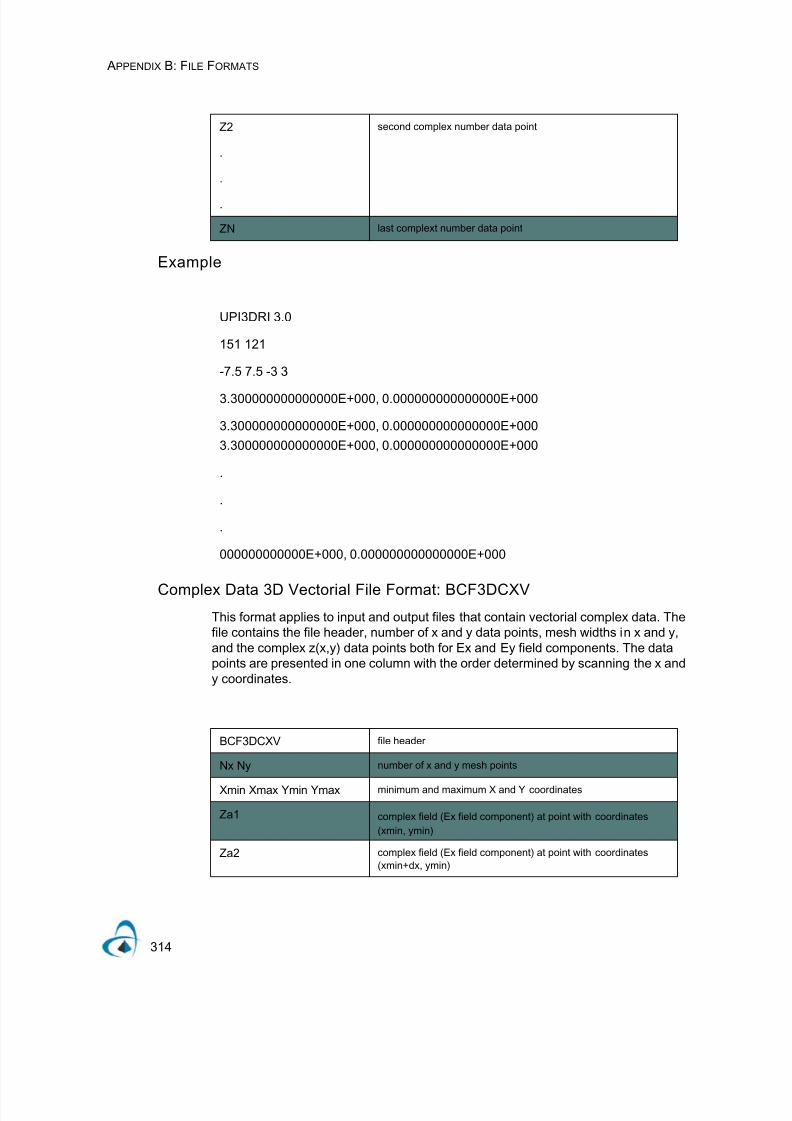
7/21/2019 OptiMode User Reference
http://slidepdf.com/reader/full/optimode-user-reference 318/339
APPENDIX B: FILE FORMATS
314
Example
Complex Data 3D Vectorial File Format: BCF3DCXV
This format applies to input and output files that contain vectorial complex data. Thefile contains the file header, number of x and y data points, mesh widths in x and y,and the complex z(x,y) data points both for Ex and Ey field components. The datapoints are presented in one column with the order determined by scanning the x andy coordinates.
Z2
.
.
.
second complex number data point
ZN last complext number data point
UPI3DRI 3.0
151 121
-7.5 7.5 -3 3
3.300000000000000E+000, 0.000000000000000E+000
3.300000000000000E+000, 0.000000000000000E+000
3.300000000000000E+000, 0.000000000000000E+000
.
.
.
000000000000E+000, 0.000000000000000E+000
BCF3DCXV file header
Nx Ny number of x and y mesh points
Xmin Xmax Ymin Ymax minimum and maximum X and Y coordinates
Za1 complex field (Ex field component) at point with coordinates
(xmin, ymin)
Za2 complex field (Ex field component) at point with coordinates
(xmin+dx, ymin)

7/21/2019 OptiMode User Reference
http://slidepdf.com/reader/full/optimode-user-reference 319/339
APPENDIX B: FILE FORMATS
315
where N=Nx*Ny, dx=(xmax-xmin)/(Nx-1), and dy=(ymax-ymin)/(Ny-1).
Note: The total number of data points is twice the number of the total mesh pointsNt=2*N.
Za3 complex field (Ex field component) at point with coordinates
(xmin+2dx, ymin)
.
ZaNX complex field (Ex field component) at point with coordinates
(xmax, ymin)
ZaNX+1
.
.
complex field (Ex field component) at point with coordinates(xmin, ymin+dy)
ZaN (N=Nx*Ny) complex field (ex field component) at point with coordinates(xmax, ymax)
Zb1 complex field (Ey field component) at point with coordinates(xmin, ymin+dy)
Zb2 complex field (Ey field component) at point with coordinates
(xmin+dx, ymin)
Zb3
.
complex field (Ey field component) at point with coordinates(xmin+2dx, ymin)
ZbNX complex field (Ey field component) at point with coordinates
(xmax, ymin)
ZbNX+1
.
.
complex field (Ey field component) at point with coordinates
(xmin, ymin+dy)
ZBN (N=Nx*Ny) complex field (Ey field component) at point with coordinates
(xmax, ymax)

7/21/2019 OptiMode User Reference
http://slidepdf.com/reader/full/optimode-user-reference 320/339
APPENDIX B: FILE FORMATS
316

7/21/2019 OptiMode User Reference
http://slidepdf.com/reader/full/optimode-user-reference 321/339
APPENDIX C: P ARSER SUPPORTED FUNCTIONS
317
Appendix C: Parser supported functions
The following functions are supported by the internal parser of OptiMode. They arenot available in the Script page because that environment expects standard VisualBasic. Use these functions in the Expression fields of Waveguide Properties dialogboxes, or as the User Variables and Functions definitions. They may also be used inthe User Function Profile definitions, in the Function Body or Limits fields. Theseparser functions are independent of VB Script. In the Scripting page of OptiMode,please use only VB Script functions. See the OptiMode Visual Basic Reference Guidefor more information on VB functions.
Supported functions
abs( x ) absolute value of x: |x|
arccos({-1..1}) return values range: 0 to π radians
arcsin({-1..1}) return values range: – π/2 to π/2 radians
arctan( x ) return values range: – π/2 to π/2 radians
arccosh({1…}) return values type: [rad]
arcsinh({0…}) return values type: [rad]
arctanh({-1..1}) return values type: [rad]
bessJ0( x ) Bessel function of the first kind: order 0
bessJ1( x ) Bessel function of the first kind: order 1
bessJn( n, x ) Bessel function of the first kind: order n
bessY0( x ) Bessel function of the second kind: order 0
bessY1( x ) Bessel function of the second kind: order 1
bessYn( n, x ) Bessel function of the second kind: order n
ceiling(x) returns the smallest integer greater or equal x
cerf(x) complementary error function for x (see erf(x) function)
cos(x) cosine of x
cosh(x) hyperbolic cosine of x
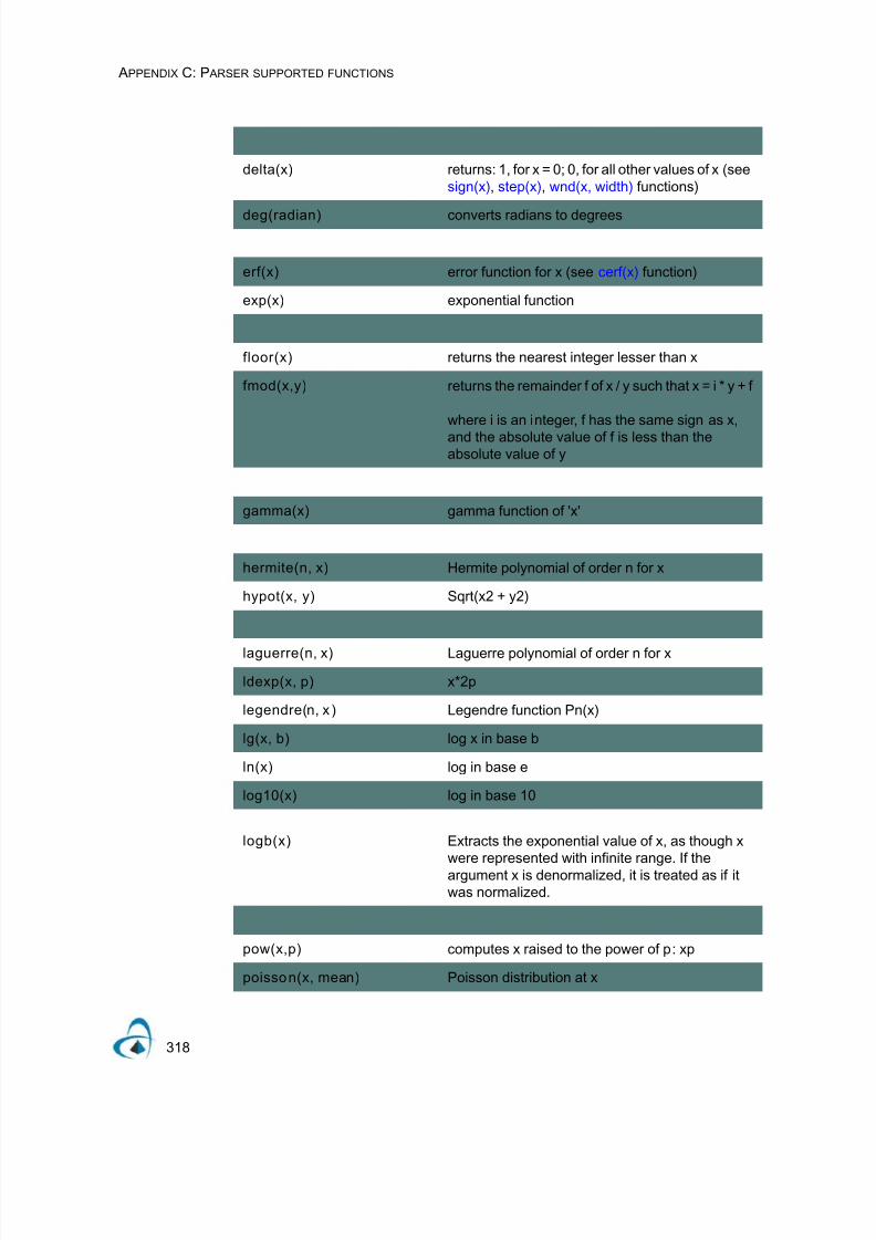
7/21/2019 OptiMode User Reference
http://slidepdf.com/reader/full/optimode-user-reference 322/339
APPENDIX C: P ARSER SUPPORTED FUNCTIONS
318
delta(x) returns: 1, for x = 0; 0, for all other values of x (seesign(x), step(x), wnd(x, width) functions)
deg(radian) converts radians to degrees
erf(x) error function for x (see cerf(x) function)
exp(x) exponential function
floor(x) returns the nearest integer lesser than x
fmod(x,y) returns the remainder f of x / y such that x = i * y + f
where i is an integer, f has the same sign as x,
and the absolute value of f is less than theabsolute value of y
gamma(x) gamma function of 'x'
hermite(n, x) Hermite polynomial of order n for x
hypot(x, y) Sqrt(x2 + y2)
laguerre(n, x) Laguerre polynomial of order n for x
ldexp(x, p) x*2p
legendre(n, x ) Legendre function Pn(x)
lg(x, b) log x in base b
ln(x) log in base e
log10(x) log in base 10
logb(x) Extracts the exponential value of x, as though xwere represented with infinite range. If theargument x is denormalized, it is treated as if itwas normalized.
pow(x,p) computes x raised to the power of p: xp
poisson(x, mean) Poisson distribution at x

7/21/2019 OptiMode User Reference
http://slidepdf.com/reader/full/optimode-user-reference 323/339
APPENDIX C: P ARSER SUPPORTED FUNCTIONS
319
rad(degree) converts degrees to radians
sign0(x) return values:
-1 for x < 0
0 for x = 0
+1 for x > 0
(see step(x), wnd(x, width), delta(x), sign(x) functions)
sign(x) return values:
-1 for x < 0
+1 for x >= 0
(see step(x), wnd(x, width), delta(x), sign0(x) functions)
sin(x) sine function of x, x [rad]
sinc(x) Sin(x) / x, x [rad]
sinh(x) hyperbolic sine function of x, x [rad]
sqr(x) power 2 of x
sqrt(x) square root of 'x'
step(x) returns:
0 for x < 0
+1 for x >= 0
(see sign(x), delta(x), wnd(x, width) functions)
tan(x) tangent function of x, return values range:
{0..inf}, x [rad]
tanh(x) hyperbolic tangent function of x, x [rad]
tcheby(order, x) Tchebychev function for x

7/21/2019 OptiMode User Reference
http://slidepdf.com/reader/full/optimode-user-reference 324/339
APPENDIX C: P ARSER SUPPORTED FUNCTIONS
320
wnd1(x) window function (window width = 1), returns:
+1 for x in the range of: < -1/2 , +1/2 >
0 for x outside the range
(see step(x), sign(x), delta(x), wnd(x, width) functions)
wnd(x, width) window function, returns:
+1 for x in the range of < -width/2 , +width/2 >
0 for x outside the range
(see step(x), sign(x), delta(x), wnd1(x) functions)

7/21/2019 OptiMode User Reference
http://slidepdf.com/reader/full/optimode-user-reference 325/339
APPENDIX C: P ARSER SUPPORTED FUNCTIONS
321
Mathematical constants
Physical constants
pi = 3.141592653589793238462643
e = 2.718281828459045235360287
euler = 0.577215664901532860606512
catalan = 0.915965594177219015054604
goldenRatio = 1.618033988749894848204587
_c = 2.9979e8 [m/s] Speed of light in free space
_e = 8.8542e-12 [F/m] Permittivity in free space
_mi = 4*pi*10e-7 [H/m] Permeability in free space _kT = 25.853 [meV] Thermal energy
_NA = 6.022045e23 Avogadro number
_kB = 1.3807e-23 [J/K] Boltzmann constant
_h = 6.626e-34 [Js] Planck constant
_hr = 1.05459 e-34 [Js] Reduced Planck Constant
_lc = 2.4263096e-1 [m] Compton wavelength of electron
_Ry = 13.6058 [eV] Rydberg energy
_ri = 1.09737312e7 [1/m] Rydberg constant
_q = 1.60219e-19 [C] Elementary charge
_me = 9.1095e-31 [kg] Free electron mass
_u = 1.660531e-27 [kg] Atomic mass unit
_mp = 1.672614e-27 [kg] Proton rest mass
_mn = 1.674920e-27 [kg] Neutron rest mass
_f = 9.648 6e4 [C/mol] Faraday constant
_a0 = 5.2917715e-11 [m] Bohr radius
_re = 2.817939e-15 [m] Electron radius
_mb = 9.274096e-24 [J/T] Bohr magnetron

7/21/2019 OptiMode User Reference
http://slidepdf.com/reader/full/optimode-user-reference 326/339
APPENDIX C: P ARSER SUPPORTED FUNCTIONS
322
System variables
System variables are related to the selected waveguide and its closest neighbour.
_d distance between the selected waveguide and its
closest neighbour
_dx distance from the selected waveguide center
_sdx signed distance from the selected waveguidecentre (-ve on left, +ve on right)
_dy distance from the substrate cladding interface
_W width of the selected waveguide
_W1 width of the closest neighbour
_x waver x coordinate
_y wafer y coordinate
_z wafer z coordinate measured from the beginningof the layout
_Ere real part of the field component
_Eim imaginary part of the field component
_EE sum of squares of field components: _Ere2 + _Eim2
_Emod magnitude of the field component:(sqrt (_Ere2 + _Eim2 ) )
_Polariz polarization: 0 = TE, 1 = TM
_Wavelen wavelength
_N_real real part of current value of refractive index
_N_real imaginary part of current value of refractive index

7/21/2019 OptiMode User Reference
http://slidepdf.com/reader/full/optimode-user-reference 327/339
APPENDIX C: P ARSER SUPPORTED FUNCTIONS
323
Figure 182 System variables definit ion
Figure 183 _sdx Definition
Notes
_dx is the distance from the waveguide centre. Use of this variable will always makewaveguides symmetric about the center. Use _sdx if an unsymmetric waveguide is tobe made.
_N_real and _N_imaginary are sometimes useful when waveguides overlap. Forexample if waveguides are made by a non-linear process that occurs on exposure to
high energy radiation, and the point in question has been exposed by two processes,then the refractive index assumed will be the refractive index from the more intenseexposure. If _N_real and _N_imaginary are observable in the User Function Profiledefinition, suitable logic can be written to get each point to assume the correct valueof refractive index. For each point in the transverse plane, the waveguides areconsidered one at a time, and the appropriate refractive index applied. If the _N_realand _N_imaginary are observed at each profile application, the existing refractive
Wafer cross-section with 2 waveguides
substrate
cladding
(_x,_y,_z)
_dx
_dy
WW1
_d

7/21/2019 OptiMode User Reference
http://slidepdf.com/reader/full/optimode-user-reference 328/339
APPENDIX C: P ARSER SUPPORTED FUNCTIONS
324
index can be compared to the refractive index generated by the current profile, andthe update will occur only if the new refractive index is greater than the existing one.More sophisticated algorithms could be implemented, if required.
Function Limits and _FnRslt_
You can limit your function by specifying the argument limits, for example enter theexpression: x*x+y*y<1 to limit the function domain by a circle of radius 1. You can alsolimit the function by using the variable _FnRslt_ which is the function value. Forexample, enter the Limits expression: abs(_FnRslt_)<1 to assure that your function isclipped when its absolute value is equal or exceeds 1. After pressing Add/Apply youadd your function definition to the list of user functions. _FnRslt_ represents a resultvalue of the base function execution for given set of arguments. Predefined for use inthe Domain Function expressions.
Examples
Expression:
ln(-x)+ln(x)
will result in "out of domain" message when validated. During execution time it willreturn zero as the result of expression evaluation. See the picture below
The same behavior will result from the following example of user defined functions.
Expression:
Fnc(x) = fncA(x)+fncB(x)
where
The fncA(x) exists only for x values smaller than 10, the fncB(x) exists for x values
greater than 10. The Fnc(x) domain is a "sum" of compound functions domains,excluding each other. In effect there is no x, which could satisfy both domainsrequirements, causing Fnc(x) always returning zero when executed, or "out ofdomain" message when validated (see Figure 184).
ATTENTION
The Function Limits describes function's domain, i.e.: function does not existsoutside the specified area. Special care should be taken when building
expressions with use of functions, so the don't exclude each other.
fncA(x) = 2*x Function Limits: x < 10
fncB(x) = x/2 Function Limits: x > 10

7/21/2019 OptiMode User Reference
http://slidepdf.com/reader/full/optimode-user-reference 329/339
APPENDIX C: P ARSER SUPPORTED FUNCTIONS
325
Figure 184 Variables and Functions dialog box

7/21/2019 OptiMode User Reference
http://slidepdf.com/reader/full/optimode-user-reference 330/339
APPENDIX C: P ARSER SUPPORTED FUNCTIONS
326
Operators and their precedence
Table 1 below lists operators and their precedence and associativity values. The linesseparate precedence levels. The highest precedence level is at the top of the table.
Table 1 Operators—Precedence and associativity values
Symbol Name or meaning Associativity
Highest precedence
() Function call
– Unary minus
+ Unary plus
* Multiply left to right
/ Divide
+ Add left to right
– Subtract
< Less than
< = Less than or equal to
> Greater than
> = Greater than or equal to
== Equal left to right
!= Not equal
= Assignment right to left
Lowest precedence

7/21/2019 OptiMode User Reference
http://slidepdf.com/reader/full/optimode-user-reference 331/339
APPENDIX D: CREATING A DLL PROFILE
327
Appendix D: Creating a DLL profile
Overview A Waveguide Profile can be implemented using a Win 32 Microsoft Dynamic LinkLibrary (DLL). These profiles are known as User DLL Profiles. A User DLL Profile isdefined using one or two functions: a Profile Function and an optional Limit Function.These functions are described in the Profile Designer chapter. Each function isdefined in a similar way. For this discussion, we will normally not distinguish betweenthe Profile and Limit Functions. The following restrictions apply to the DLL used byUser DLL Profiles. Functions implemented using Microsoft 'C' version 6 or greater aresupported. However, it should be possible to use other languages as long as aproperly formatted DLL is created. If a Limit Function is used, it must reside in thesame DLL that contains the Profile Function. Creating a DLL for use with a User DLLProfile is a three-phase process called the 'build process'. The phases of the build
process are:• Edit
• Compile
• Link
Phase 1: Edit
The first step in creating a DLL for use with a User DLL Profile is to create the Cprogramming instructions that will be used to define the profile. Any text editor can beused to enter the C instructions. The editor provided by Microsoft's Visual Studio iswell suited to this purpose. The C instructions are stored in a file with a '.c' fileextension. This file is called a source file. The function name and the parameters tothat function are defined in the User DLL Profile View in the Profile Designer. You mustcreate a function whose function name and parameter list matches the parametersspecified in the User DLL Profile View.
Each parameter will have a type 'double' and the function must return a double value.The Profile Function and Limit Function can call other functions. These functions canbe created by you or can be packaged in a third party library. Many source filescontaining many functions can be used to implement a User DLL Profile. The onlyrestriction is that at least one of those functions must match the name and parameterlist of the Profile Function specified in the User DLL Profile. If a Limit Function is used,then at least one of these functions must match the name and parameter list of thisfunction.
Phase 2: Compile.
The C code created in phase 1 can be compiled using a C or C++ compiler such asMicrosoft Visual C++. However, the code must be compiled as C code. This meansthe source file extension must be '.c'. The Microsoft C++ compiler will compile fileswith a '.c' extension as C code. No C++ constructs can be used in the Profile Functionor Limit Function. The compiler will report any errors or warnings discovered while
7/21/2019 OptiMode User Reference
http://slidepdf.com/reader/full/optimode-user-reference 332/339
APPENDIX D: CREATING A DLL PROFILE
328
parsing the source file(s). Any errors must be corrected by returning to the edit phasethe process. The
Edit and Compile phases of the process must be repeated until all source files compilewithout error.
Phase 3: Link
The compiled C code is then passed to a linker for the final link phase of the buildprocess. This phase creates the file with the '.dll' extension that is specified in the 'DLLfile name' field of the User DLL Profile view. As in the compile stage, the linker mayencounter errors. These errors must all be corrected before the dynamic link library iscreated.
Summary
The complexity of the User DLL profile is limited by the capabilities of the compiler andthe software development skills of the user. If necessary, multiple functions spanning
multiple files can be used to create the profile function. Optiwave supports this featurefor the Microsoft C compiler. However, you should be able to build the DLLs with anycompiler supporting DLL creation. Use of other compilers may require someexperimentation with compilation and linking options.
Creating a dynamically linked library (DLL) for User DLL profile using
Microsoft Visual Studio VC6++
To create a .dll suitable for OptiMode User DLL profiles using Microsoft Visual StudioVC6++, perform the following procedure:
Step Action
1 Select File > New to create a new win32 dll project.
2 On the Projects tab, select Win32 Dynamic-Link Library.
3 Specify a file name, for example UserDLL.
4 Click OK.
5 Select An Empty Dll Pro jec t.
6 Click Finish and OK.
7 Manually add .c and .h files to the project (for example, testdll.c andtestdll.h).
Note: testdll.h contains declarations of the functions to be exported.Make sure that the declaration is preceded by the following directive

7/21/2019 OptiMode User Reference
http://slidepdf.com/reader/full/optimode-user-reference 333/339
APPENDIX D: CREATING A DLL PROFILE
329
= __dec lspec(dl lexport )‘. If not, the function is not going to be exported.testdll.cpp contains function definitions.
8 Build the .dll file.
Alternatively, you can use the template project (UserDLL.dsp ) distributed with
OptiMode (see samples directory) and simply update the dll functions according toyour needs.

7/21/2019 OptiMode User Reference
http://slidepdf.com/reader/full/optimode-user-reference 334/339
APPENDIX D: CREATING A DLL PROFILE
330

7/21/2019 OptiMode User Reference
http://slidepdf.com/reader/full/optimode-user-reference 335/339
APPENDIX E: B ATCH PROCESSING
331
Appendix E: Batch Processing
OverviewThe Batch Processing feature is useful for projects that take a long time for thesimulation to finish. Instead of starting the simulation from the OptiMode Designer inan interactive session, the simulations can be listed in a batch file. Running the batchfile will start each simulation in the order of the list. This will create a series of analyzerfiles (and, if requested, batch processing log files) that can be reviewed at a later time.The analyzer .m3a files will be written to the current directory. If you want to view theindividual data files, you manually start the analyzer, and open the .m3a data files.
Stucture of the Batch Command Line
The first word in the command line (required) is the name of the OptiMode simulator
executable file, Opt i Mode_Sol ver . This is followed by a sequence of switches forspecifying which OptiMode simulator to use, which project file (.mxd file) to use, andother options in the batch simulation. To let the computer know where to find the fileOpt i Mode_Sol ver . exe, you need to set the path to that file, e.g. “C:\Program Files(x86)\Optiwave Software\OptiBPM 12\bin” (or wherever you have installed OptiModeon your computer).
The second word in the command line (required) is a switch specifying whichsimulator you would like to call. The table below lists all the switch names for all thesimulators:
Table, Switches for specifying mode solvers
The third word in the command line (optional) is /BATCH. This will direct output tostdout (which usually contains comments on the run-time progress) away from theNotification window in the Analyzer file. Used alone, the stdout comments will go tothe window with the batch file. These comments can also be redirected to a file withthe /LOG switch (see below).
Mode Solving Simulator Switch
Real valued modes by ADI method /SOLVEREALADI
Complex modes by ADI method /SOLVECOMPLEXADI
Modes in anisotropic materials /SOLVEANISO
Vector modes in fibres /SOLVEFIBREVECTOR
LP modes in fibres /SOLVEFIBRELP
Modes by the finite difference method /SOLVECOMPLEXFD

7/21/2019 OptiMode User Reference
http://slidepdf.com/reader/full/optimode-user-reference 336/339
APPENDIX E: B ATCH PROCESSING
332
The next word in the command line (required) is the path and project file name. It is astring contained in quotation marks, e.g.“C: / Fol der A/ Fol der B/ pr oj ect name. mxd”.
The next two words are optional: /LOG and a path and file name for the log data, e.g.
“C: / Fol der A/ Fol der B/ l ogf i l e. l og” If no file name is specified, a default onewill be used: Opt i LogFi l e. l og. The messages document any warnings as well asany errors that may have resulted in the solving not continuing to completion. Theformat of the stdout file starts with the name of the solver file, and is followed by thesolver type. Each output message is streamed to stdout until the solver has exited,either by error or successfully. This exit is also logged to stdout. All the messages aretime stamped, and no extraneous system or 3rd party data is added to the log fileunless it is relevant to the success or failure of the simulation.
Examples of logged exiting scenarios:
• Normal termination: end of simulation
• Security error: protection key not found, invalid server
• Application failure: user closes application, out of memory or hard drive space• Design problems: mode not found, insufficient data for simulation
Example of a Batch Processing File
Opti Mode_Sol ver / SOLVEREALADI / BATCH "C: \ r eal Sol veTest . mxd" / LOG test _l ogf i l e. l ogOpti Mode_Sol ver / SOLVECOMPLEXADI / BATCH "C: \ compl exSol veTest . mxd" / LOG test _l ogf i l e. l ogOpti Mode_Sol ver / SOLVEANI SO / BATCH "C: \ r eal Sol veTest . mxd" / LOG test _l ogf i l e. l ogOpti Mode_Sol ver / SOLVEFI BREVECTOR / BATCH "C: \ r eal Sol veTest . mxd" / LOG t est _l ogf i l e. l ogOpti Mode_Sol ver / SOLVEFI BRELP / BATCH "C:\ r eal Sol veTest . mxd" / LOG t est_ l ogf i l e. l og
Example of stdout output, format in ascii
*** Fr i Mar 26 14: 17: 52: START – Opt i Mode_Sol ver
Fr i Mar 26 14: 17: 52: Fi l e: C: \ r eal Sol veTest . mxd
Fr i Mar 26 14: 17: 52: The cur r ent out put f i l e i sC: \ r eal Sol veTest I . m3a
Fr i Mar 26 14: 17: 55: I t er at i on 1 st ar t ed. Fri Mar 26 14: 18: 25:I t er at i on 1 f i ni shed successf ul l y.
*** Fri Mar 26 14: 18: 25: End - Si mul at i on f i ni shed
Automatic loading of VB script from command l ine
Automatic loading of VB script from command line (BATCH mode) allows loading oftext files containing VB script. The feature is intended for the users who develop anumber of VB script files or modify them dynamically in-between solving. The idea isvery simple: Solver loads a Layout Design project, and into its space, loads contentof a text file, containing VB script. Solves start with execution of the VB script, in thesame way as solves of a regular project file equipped with a script.

7/21/2019 OptiMode User Reference
http://slidepdf.com/reader/full/optimode-user-reference 337/339
APPENDIX E: B ATCH PROCESSING
333
Command line syntax
The command line syntax supporting automatic loading of VB script files is thefollowing:
/SCRIPT::VBS_Filename
where VBS_Filename is the file whose contents will be read into the internal Scriptbuffer. If the file name contains spaces, the file name must be surrounded by quotationmarks. For example."My VB Scrtipt.txt".
Notes:
There are no spaces between the /SCRIPT command, the two colons or the file name.
The file name can contain the file path and drive letter, or it can be a relative path.
If the path and drive letter are omitted, an attempt to open the file in the currentdirectory (where the batch file/command is being executed) is made.
If no file of that name exists in the current directory, an attempt to open a file of thatname in the folder that contains the layout project file is made.
If this fails, the file cannot be located and an error will be reported and the solving willstop.
The VB script will execute when the solver is invoked. The 'Solve Using Script' solveoption is automatically asserted when the /SCRIPT:: command line option isencountered. Any existing script stored in the layout project file is replaced by thecontents of the loaded-in script file.
Batch command examples
The following are sample batch commands that instruct the application to load VBScript code from files:
Opti Mode_Sol ver / SOLVEREALADI / BATCH / SCRI PT: : "C:\ Proj ects\ VBScr i pt . t xt" "C: \ Proj ects\ t estPr oj ect . mxd"
In the following example, the VB Script code file is expected to be in the same folderas the Layout Design data file. If the script code file name contains spaces, make sureto surround it with quotes (""):
Opti Mode_Sol ver / SOLVEREALADI / BATCH / SCRI PT: : "VBScr i pt. t xt" "C: \ Proj ects\ t estPr oj ect . mxd"

7/21/2019 OptiMode User Reference
http://slidepdf.com/reader/full/optimode-user-reference 338/339
APPENDIX E: B ATCH PROCESSING
334

7/21/2019 OptiMode User Reference
http://slidepdf.com/reader/full/optimode-user-reference 339/339