optimization of the axial porosity … · the liquid-piston compressor is used for compressed air...

1 Copyright © 2013 by ASME

Proceedings of the ASME 2013 International Mechanical Engineering Congress and Exposition IMECE2013

Nov. 15-21, 2013, San Diego, CA, USA

IMECE2013-63862

OPTIMIZATION OF THE AXIAL POROSITY DISTRIBUTION OF POROUS INSERTS IN A LIQUID-PISTON GAS COMPRESSOR USING A ONE-DIMENSIONAL FORMULATION

Chao Zhang Department of Mechanical

Engineering University of Minnesota Minneapolis, MN55414

Terrence W. Simon Department of Mechanical


Perry Y. Li Department of Mechanical


[email protected] [email protected] [email protected]

ABSTRACT A One-Dimensional (One-D) numerical model to calculate

transient temperature distributions in a liquid-piston compressor

with porous inserts is presented. The liquid-piston compressor is

used for Compressed Air Energy Storage (CAES), and the

inserted porous media serve the purpose of reducing temperature

rise during compression. The One-D model considers heat

transfer by convection in both the fluids (gas and liquid) and

convective heat exchange with the solid. The Volume of Fluid

(VOF) method is used in the model to deal with the moving

liquid-gas interface. Solutions of the One-D model are validated

against full CFD solutions of the same problem but within a

two-dimensional computation domain, and against another study

given in the literature.

The model is used to optimize the porosity distribution, in

the axial direction, of the porous insert. The objective is to

minimize the compression work input for a given piston speed

and a given overall pressure compression ratio. The model

equations are discretized and solved by a finite difference

method. The optimization method is based on sensitivity

calculations in an iterative procedure. The sensitivity is the

partial derivative of compression work with respect to the

porosity value at each optimization node. In each optimization

round, the One-D model is solved as many times as there are

optimization nodes, and each time the porosity value at a single

optimization node is changed by a small amount. From these

calculations, the sensitivity of changing the porosity distribution

to the total work input (objective) is obtained. Based on this, the

porosity distribution is updated in the direction that favors the

objective. Then, the optimization procedure marches to the next

round and the same calculations are completed iteratively until

an optimum solution is reached. The optimization shows that

porous media with high porosity should be used in the lower

part of the chamber and porous media with low porosity should

be used in the upper part of the chamber. An optimal distribution

of porosity over the chamber is obtained.

1. INTRODUCTION Liquid-piston gas compressors with porous inserts can be

used for Compressed Air Energy Storage (CAES). In

power-producing systems, the CAES approach is used in order

to overcome the mismatch between power demand and power

generation, [1] and [2], by storage and discharge. During low

power demand periods, excess power is used to compress air

and the compressed air is stored in a vessel. During high power

demand periods, the compressed air is expanded to output work.

An important characteristic of efficient and effective CAES

operation is near-isothermal compression, as discussed in [2] –

[6]. The main reason for this is that compression typically

results in a temperature rise of the air and the extra thermal

energy due to the temperature rise is wasted during the storage

period as the compressed air cools to the ambient temperature.

Therefore, in order to reduce temperature rise during

compression, porous media, which have large surface areas per

volume, are inserted into the liquid-piston gas compressor. The

term “liquid-piston” implies that the compression of the gas is

done with a rising liquid-gas interface created by pumping

liquid into the lower section of the compression chamber. A

previous study has shown that liquid-piston has an advantage

over traditional solid piston in terms of power consumption [7].

Another advantage of the liquid piston is that it does not

compromise volume compression ratio, as the liquid can flow

through the porous media and can be effectively cooled by the

media.

The present study develops a one-dimensional (One-D)

numerical model for the liquid-piston compressor with porous

inserts. Although higher-dimensional CFD studies on related

subjects have already been done and they can resolve in detail

the flow fields [8] – [12], the One-D numerical model is far less


computationally expensive, and is therefore easier to utilize in

the optimization analysis.

In the past, many studies have been done to investigate

simplified numerical models for regenerative heat exchangers

that operate in cycles. Each cycle consists of a cooling phase

and a heating phase. In the present study, the porous inserts play

the same role as regenerative heat exchangers when the

exchangers are operating in the cooling phase to cool the fluid.

An early simplified model of regenerative heat exchangers

couples the spatial advection of fluid energy with the transient

storage of energy in the solid, and solves the equations [13]. By

using superposition methods, the solution is extended to solve

various thermal entry problems [14]. Regenerative heat

exchanger analysis in a system that uses by-pass flow to control

the outlet gas temperature was solved in [15] and [16].

Optimization was introduced to maximize thermal efficiency of

the heating phase of a regenerative heat exchanger [17]. Effects

of residual gas from the previous cycle in the exchangers are

modeled in [18]. Two bulk average heat transfer coefficients,

one being linearly proportional to the gas flow rate, and the

other being linearly proportional to the surface heat transfer

coefficient, are analyzed and compared in [19]. Improved

numerical method to solve the same equations employing

Richardson extrapolation was introduced in [20]. The modeling

to include the transient change of gas temperature was

introduced in [21] – [23]. The model is further improved by

including thermal conduction in the solid in the direction

parallel to the flow [24].

Compared to the present study, the major differences of the

flow situations in the aforementioned literature [13] – [24] are:

(1) the air is not compressed to high pressure ratio in the

exchangers, and (2) there is no moving liquid-air interface in the

exchangers. A one-energy-equation, zero-dimensional (Zero-D)

model for compression of air in a long, thin channel has been

proposed for modeling compression [25]. This model was

further developed into a two-energy-equation, Zero-D model to

simulate liquid-piston compression in a chamber filled with

interrupted-plate heat exchangers, for solution of the transient

temperatures of both the fluid and solid of the exchanger [26].

Yet, in [25] and [26], the numerical models are not capable of

calculating transient spatial distributions of temperature since

they are Zero-D models.

In order to model the liquid-piston compression in a

one-dimensional fashion, the Volume of Fluid (VOF) method

[27] is used. The VOF method tracks bulk locations of liquid

and gas by solving volume fraction scalar fields. This concept is

used in the One-D model in the present study to handle the

moving liquid-air interface (liquid-piston surface).

2. THE ONE-D NUMERICAL MODEL 2.1. Governing Equations

The compression process in a liquid piston air compressor

is formulated considering time variations and spatial variations

in the chamber axial direction. A schematic of the compressor is

shown in Fig. 1. Water is pumped into a chamber filled with

porous inserts to compress the air. At the beginning of the

compression process, the water-air interface starts at the bottom

of the chamber. The spatial-average of the inlet water velocity

has a constant value of 𝑈0. Since water is incompressible, it is

assumed that the water-air interface also moves at velocity 𝑈0 .

The water-air interface position at any time during compression

is,

𝑥𝑝 = 𝑥𝑝(𝑡) = 𝑈0𝑡 (1)

The velocity of air is

assumed to be linearly

distributed along the 𝑥

axis, matching the water

(interface) velocity at the

water-air interface, and

zero at the top cap. The

velocity field of air and

water are given by,

𝑢 = 𝑢(𝑥, 𝑡) =

{𝑈0, 𝑥 < 𝑥𝑝

𝑈0𝐿−𝑥

𝐿−𝑥𝑝, 𝑥 ≥ 𝑥𝑝

(2)

Using the VOF method, volume fractions of air and water

are defined. The volume fraction is a scalar function that gives

the fraction of volume occupied by a single phase at a location.

The sum of volume fractions of the two phases at any location

equals 1.

𝛼1 + 𝛼2 = 1 (3)

where subscripts 1 and 2 refer to the air and water phase,

respectively.

The volume fraction values track bulk locations of the

water and air phases. Velocity fields and temperature fields are

shared by the two phases. The continuity equation for air is,

𝜕𝛼1𝜌1

𝜕𝑡+

𝜕𝛼1𝜌1𝑢

𝜕𝑥= 0 (4)

Since water is incompressible, the continuity equation of water

gives,

𝜕𝛼2

𝜕𝑡+

𝜕𝛼2𝑢

𝜕𝑥= 0 (5)

The energy transport in the fluid mixture, which is made up of

immiscible water and air, is governed by,

𝜖𝜕𝜌𝑐𝑝 𝑇

𝜕𝑡+ 𝜖

𝜕𝜌𝑐𝑝 𝑢𝑇

𝜕𝑥

= 𝑘𝜖𝜕2𝑇

𝜕𝑥2+ 𝛼1𝛽1𝑇(

𝜕𝑝

𝜕𝑡+ 𝑢

𝜕𝑝

𝜕𝑥) + ℎ𝑉(𝑇𝑠 − 𝑇)

(6)

where,

𝜌𝑐𝑝 = 𝛼1𝜌1𝑐𝑝,1 + 𝛼2𝜌2𝑐2 (7)

𝑘 = 𝛼1𝑘1 + 𝛼2𝑘2 (8)

Fig. 1. Schematic of compressor


When solving Eq. (6), the pressure in the work terms can be

substituted by temperature and air density using the ideal gas

law,

𝑝 = 𝜌1𝑅𝑇 (9)

The energy transport in the solid is given by,

(1 − 𝜖)𝜌𝑠𝑐𝑠𝜕𝑇𝑠

𝜕𝑡= 𝑘𝑠(1 − 𝜖)

𝜕2𝑇𝑠

𝜕𝑥2− ℎ𝑉(𝑇𝑠 − 𝑇) (10)

Equations (4), (5), (6), and (10) are the governing equations of

fluid flow in a liquid-piston air compressor with porous inserts.

The boundary conditions are:

𝑢(𝑥 = 0) = 𝑈0 (11)

𝑢(𝑥 = 𝐿) = 0 (12)

𝑇(𝑥 = 0) = 𝑇(𝑥 = 𝐿) = 𝑇0 (13)

The isothermal temperature condition on the wall (𝑥 = 𝐿) is

used in the numerical model. The main reason for this is that: (1)

in applications, the compressor wall is usually made of metal,

which has much larger thermal capacity and density than air,

and thus the wall would require much more heat absorption to

increase its temperature than air would, and (2) the compression

time is usually in just seconds, which is too short a time period

for the compressor wall to heat up.

The energy equations of the fluid and solid are coupled

through interfacial heat transfer. Kamiuto and Yee proposed a

heat transfer correlation for porous media [28], which gives a 40%

uncertainty compared to sixteen sets of experimental data on

different porous media. The correlation is further converted to

be based on the length scale pore size by [29], which is then

used in [12] for a metal foam of 93% porosity. The correlation is

given by,

𝑁𝑢𝑉 =ℎ𝑉𝐷𝑝

2

𝑘= 0.996(

𝜌𝜖𝑢𝐷𝑝

𝜇𝑃𝑟)0.791 (14)

Parameter 𝐷𝑝 is a characteristic length based on the pore

structure of the porous medium. It is 3.61mm in the present

study. It is assumed that the heat transfer between air and solid

and the heat transfer between water and solid follow the same

dimensionless heat transfer correlation. The fluid mixture

density, viscosity and Prandtl number are given by,

𝜌 = 𝛼1𝜌1 + 𝛼2𝜌2 (15)

𝜇 = 𝛼1𝜇1 + 𝛼2𝜇2 (16)

𝑃𝑟 = 𝛼1𝑃𝑟1 + 𝛼2𝑃𝑟2 (17)

2.2. Numerical Method

Equations (4), (5), (6), and (10) are solved by a finite

difference method. The continuity equations for water and air

are discretized using an explicit upwind method. They are given

by:

𝛼2,𝑗𝑛+1 − 𝛼2,𝑗

𝑛

𝛥𝑡+𝛼2,𝑗

𝑛𝑢2,𝑗𝑛 − 𝛼2,𝑗−1

𝑛𝑢2,𝑗−1𝑛

𝛥𝑥= 0

(18)

𝛼1,𝑗𝑛+1𝜌1,𝑗

𝑛+1 − 𝛼1,𝑗𝑛𝜌1,𝑗

𝑛

𝛥𝑡

+𝛼1,𝑗

𝑛𝜌1,𝑗𝑛𝑢1,𝑗

𝑛 − 𝛼1,𝑗−1𝑛𝜌1,𝑗−1

𝑛𝑢1,𝑗−1𝑛

𝛥𝑥= 0

(19)

Because of the advection term in the transport of fluid energy

equation, it is discretized using an explicit scheme, with upwind

differencing on the advection term and central differencing on

the diffusion term.

(𝜌𝑐𝑝 𝑗

𝑛+1 − 𝛼1,𝑗𝑛+1𝜌1,𝑗

𝑛+1𝑅)𝑇𝑗𝑛+1 − (𝜌𝑐𝑝

𝑗

𝑛 − 𝛼1,𝑗𝑛 𝜌1,𝑗

𝑛 𝑅)𝑇𝑗𝑛

𝛥𝑡

+𝜌𝑐𝑝

𝑗

𝑛𝑢𝑗𝑛𝑇𝑗

𝑛 − 𝜌𝑐𝑝 𝑗−1

𝑛 𝑢𝑗−1𝑛 𝑇𝑗−1

𝑛

𝛥𝑥−ℎ𝑉𝑗

𝑛(𝑇𝑠,𝑗𝑛 − 𝑇𝑗

𝑛)

𝜖

= 𝑘𝑗𝑛 𝑇𝑗−1

𝑛 −2𝑇𝑗𝑛+𝑇𝑗+1

𝑛

𝛥𝑥2+

𝛼1,𝑗𝑛 𝜌1,𝑗

𝑛 𝑅𝑢𝑗𝑛𝑇𝑗

𝑛−𝛼1,𝑗−1𝑛 𝜌1,𝑗−1

𝑛 𝑅𝑢𝑗−1𝑛 𝑇𝑗−1

𝑛

𝛥𝑥

(20)

The energy transport in the solid is governed by diffusion. Thus

the solid energy equation is discretized using an implicit scheme,

with central differencing in space. It is given by

𝑎𝑠,𝑗𝑇𝑗−1𝑛+1 + 𝛽𝑠,𝑗𝑇𝑗

𝑛+1 + 𝜒𝑠,𝑗𝑇𝑗+1𝑛+1 = 𝛾𝑠,𝑗 (21)

where,

𝑎𝑠,𝑗 = −𝑘𝑠

𝛥𝑥2 (22)

𝛽𝑠,𝑗 =𝜌𝑠𝑐𝑠

𝛥𝑡+

2𝑘𝑠

𝛥𝑥2+

ℎ𝑣,𝑗𝑛+1

1−𝜖𝑗 (23)

𝜒𝑠,𝑗 = −𝑘𝑠

𝛥𝑥2 (24)

𝛾𝑠,𝑗 =𝜌𝑠𝑐𝑠

𝛥𝑡𝑇𝑠,𝑗

𝑛 +ℎ𝑣,𝑗

𝑛+1

1−𝜖𝑗𝑇𝑗

𝑛+1 (25)

Let the computational domain be discretized by 𝑁𝑛 number of

nodes; 0 denotes the node at 𝑥 = 0, and 𝑁𝑛 − 1 denotes the

node at 𝑥 = 𝐿. Equation (21) is written in matrix form for all

the nodes in the computational domain:


[ 𝛽𝑠,1 𝜒𝑠,1𝑎𝑠,2 𝛽𝑠,2 𝜒𝑠,2

… … …… … 𝜒𝑠,𝑁𝑛−3

𝑎𝑠,𝑁𝑛−2 𝛽𝑠,𝑁𝑛−2]

[ 𝑇𝑠,1𝑇𝑠,2…

𝑇𝑠,𝑁𝑛−3𝑇𝑠,𝑁𝑛−2]

𝑛+1

=

[

𝛾1 − 𝑎𝑠,1𝑇𝑠,0𝛾2. . .

𝛾𝑁𝑛−3𝛾𝑁𝑛−2 − 𝜒𝑠,𝑁𝑛−1𝑇𝑠,𝑁𝑛−1]

(26)

Using the Thomas algorithm, the matrix on the LHS of Eq. (26)

is converted into an upper diagonal matrix. Then the

temperature values are solved by back substitution, starting from

node 𝑁𝑛 − 2 and moving toward node 1.

2.3. Solution and Validation

A compression problem in a liquid-piston compressor with

porous inserts is solved. The dimension of the compression

domain, compression speed, and physical properties are given in

Table 1. The thermal conductivity of air is obtained by fitting

the conductivity data (from [30]). The total compression time is

2.6 seconds. Water starts entering the compressor from the

bottom of the chamber (𝑥 = 0). The chamber is occupied by a

porous insert having an interfacial heat transfer correlation with

surrounding fluid that follows Eq. (14). The computation is run

on a mesh with 3500 axial nodes and over 30,000 time steps

(∆𝑡 = 8.667 × 10−5𝑠𝑒𝑐𝑜𝑛𝑑𝑠). A C++ code is written to solve

the governing equations.

Table 1. List of Parameters and Properties

𝐿 = 0.29

𝑐𝑝,1 = 100 (𝑘 )

𝜇2 = 1.002 × 10−3𝑃𝑎 𝑠

𝜌2 = 1000 3⁄

𝑐2 = 181. (𝑘 ) 𝑃𝑟2 = .

𝑇0 = 297

𝑈0 = 0.10 𝑠⁄

𝑃𝑟1 = 0.71

𝜌0 = 1.192 3⁄

= 287.06 (𝑘 ) 𝑘2 = 0. 6 ( ) 𝜌𝑠 = 2719 3⁄ 𝑐𝑠 = 871 (𝑘 )

𝜇1 = 1.716 × 10−5 × (𝑇

27 )2 3

𝑃𝑎 𝑠

𝑘1 = (0.00 68 06 +7.16 7 × 10−5𝑇

) ( )⁄

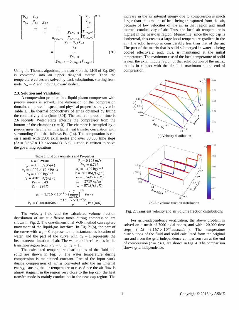
The velocity field and the calculated volume fraction

distribution of air at different times during compression are

shown in Fig. 2. The one-dimensional VOF method can capture

movement of the liquid-gas interface. In Fig. 2 (b), the part of

the curve with 𝛼1 = 0 represents the instantaneous location of

water, and the part of the curve with 𝛼1 = 1 represents the

instantaneous location of air. The water-air interface lies in the

transition region from 𝛼1 = 0 to 𝛼1 = 1.

The calculated temperature distributions of the fluid and

solid are shown in Fig. 3. The water temperature during

compression is maintained constant. Part of the input work

during compression of air is converted into the air internal

energy, causing the air temperature to rise. Since the air flow is

almost stagnant in the region very close to the top cap, the heat

transfer mode is mainly conduction in the near-cap region. The

increase in the air internal energy due to compression is much

larger than the amount of heat being transported from the air,

because of low velocities of the air in that region and small

thermal conductivity of air. Thus, the local air temperature is

highest in the near-cap region. Meanwhile, since the top cap is

isothermal, this creates a large local temperature gradient in the

air. The solid heat-up is considerably less than that of the air.

The part of the matrix that is solid submerged in water is being

cooled effectively, and, thus, is maintained at the initial

temperature. The maximum rise of the local temperature of solid

is near the axial middle region of that solid portion of the matrix

that is in contact with the air. It is maximum at the end of

compression.

(a) Velocity distribution

(b) Air volume fraction distribution

Fig. 2. Transient velocity and air volume fraction distributions

For grid-independence verification, the above problem is

solved on a mesh of 7000 axial nodes, and with 120,000 time

steps ( ∆𝑡 = 2.167 × 10−5𝑠𝑒𝑐𝑜𝑛𝑑𝑠 ). The temperature

distributions of the fluid and solid calculated from the original

run and from the grid independence comparison run at the end

of compression (𝑡 = 2.6𝑠) are shown in Fig. 4. The comparison

shows grid independence.


(a) Fluid temperature distribution

(b) Solid temperature distribution

Fig.3. Transient temperature distributions

(a) 𝑇(𝑡 = 2.6𝑠) (b) 𝑇𝑠(𝑡 = 2.6𝑠)

Fig.4. Temperature distributions at the end of compression

(𝑡 = 2.6𝑠) from the original solution and from the finer-grid

solution for grid-independence verification

For validation purposes, solutions of a two-dimensional

(Two-D), axisymmetric CFD simulation of a liquid-piston

compressor fully occupied by porous inserts are taken from [12]

and compared to the One-D solutions of the present study. The

two compression problems being solved are identical. The

radius of the chamber is 0.0254m in [12]. The radius is not of

concern to the present, One-D computation. The fluid

temperature distribution from the present One-D solution is

compared with the centerline temperature distribution from the

Two-D CFD solution, and also compared to the Two-D

temperature field in Fig. 5. The comparison shows that the

One-D model can capture the important features of the transient

axial temperature distribution of the fluid mixture in the

chamber. The Two-D temperature fields show high temperature

streaks in the region very close to the top cap. This is consistent

with the One-D solution. The physical reasons are that the flow

is mostly stagnant in that region, and the increase in the internal

energy added due to compression work is much greater than the

energy being conducted away to the solid phase in that region.

The solid temperature distributions calculated from the One-D

and Two-D solutions are shown in Fig. 6. Comparing the One-D

solid temperature distribution and the centerline temperature

distribution from the Two-D solution, one sees that the

maximum local temperature difference is less than 4K. This is

due to a lack of radial conduction in the One-D problem.

Although this difference appears large in the scaled plot, the

overall shape of the One-D solid temperature curve correctly

represents the same feature of the solid temperature distribution

from the Two-D solution.

(a) Fluid temperature, 𝑡 =2

5𝑡𝑓 = 1.0 s

(b) Fluid temperature, 𝑡 = 𝑡𝑓 = 2.6s

Fig. 5. Comparisons of fluid temperature distributions between

One-D solution and Two-D solution from [12]

Fig. 6. Comparisons of solid temperature distribution at

𝑡𝑓 = 2.6 seconds between the One-D solution and Two-D

solution from [12]


3. OPTIMIZATION USING THE ONE-D MODEL 3.1. Optimization Objective and Constraints

An optimization problem now being addressed by using the

One-D model developed in the previous section is of the

distribution of porosity inside the chamber. As mentioned earlier,

the purpose of inserting porous media in the compressor is to

reduce temperature rise during compression. From the heat

transfer point of view, a larger percentage of solid material,

which indicates lower porosity, leads to less temperature rise of

air. If the temperature rise could be minimized, less compression

work would be needed to maintain the air pressure at the storage

pressure as the compressed air cools to the ambient temperature.

If isothermal compression could be achieved, no additional

pressure work would be needed for there would be no

cool-down. On the other hand, a larger percentage of solid

material also increases flow drag due to the liquid and air

moving through the porous material, which potentially requires

more compression work to overcome. Thus, the optimization

goal is to find the porosity distribution for the porous media that

minimizes the work input. The porosity value in this problem is

bound by the values [0.7, 0.96]. A major constraint to the optimization problem is the fixed

power density. Based on the previous work in [5], [6] and [26],

the power density is the storage energy per unit volume divided

by the compression time. The storage energy is the amount of

work output as the compressed air undergoes an isothermal

expansion process. Therefore, the power density is given by:

𝑃𝑜𝑤 =𝐸𝑠

𝑉0𝑡𝑓=

𝑚𝑅𝑇0(ln(𝜁)−1+1

𝜁)

𝑉0𝑡𝑓=

𝜌0𝑅𝑇0(ln(𝜁)−1+1

𝜁)

𝑡𝑓 (27)

In the optimization problem, the power density is fixed by fixing

the compression time and the pressure compression ratio. As the

porosity distribution is gradually updated during optimization,

the compression speed also needs to be updated accordingly to

meet the requirement of fixed compression time and fixed final

pressure compression ratio.

The compression work during compression from 𝑡 = 0 to

𝑡 = 𝑡𝑓 is given by

comp = ∫ (𝑃 + 𝑃r)𝑈0𝐴dt𝑡𝑓0

(28)

This is the objective function that must be minimized. The

compression work is done to pump the liquid piston against the

thermodynamic pressure of air, 𝑃, and the flow resistance of the

porous insert, 𝑃r.

The instantaneous thermodynamic pressure of the air in the

chamber is given by,

𝑃 =1

𝐿∫ 𝛼1𝑅𝑇𝑑𝑥𝐿

0 (29)

The instantaneous air volume fraction and fluid temperature are

variables that can be obtained by solving the One-D model.

A general formulation of the flow resistance due to the

porous medium is based on Darcian and Forchheimer terms:

𝑃𝑟 = ∫ [𝜇

𝐾𝜖𝑢 +

1

2𝜌𝑏(𝜖𝑢)2] 𝑑𝑥

𝐿

0

(30)

Note that in this problem the VOF method is used, and 𝜌 and 𝜇

are the fluid mixture properties given by Eqns. (15) and (16). A

measurement taken in [12] showed that the following

parameters of Eq. (30) are suitable for a 93% porous metal foam

with 10 pores per inch (10 ppi):

= 2. 97 × 10−7 2, 𝑏 = 70.1 ⁄

Equation (30) does not account for the effect of porosity on the

flow resistance. Ergun proposed a term, (1−𝜖)2

𝜖3 , multiplied to

the Darcian velocity in the Darcian resistance term, and a term, 1−𝜖

𝜖3 , multiplied to the Darcian velocity squared in the

Forchheimer resistance term [31]. Therefore, considering

Ergun’s equation and the resistance parameters obtained in [12],

the following equation will be used to account for the effect of

porosity on flow resistance,

𝑃𝑟 = ∫ [𝜇

𝐾

(1−𝜖)2

𝜖3𝜖𝑢 +

1

2𝜌��

1−𝜖

𝜖3(𝜖𝑢)2] 𝑑𝑥

𝐿

0

(31)

where, = 1. 60 × 10−9 2, �� = 6 0.

After compression, the compressed air cools to the initial

temperature; cooling work is done to decrease its volume while

maintaining its pressure. This cooling work has been addressed

in [5], [6] and [26]. It is given by:

cool = (𝑃𝑓 − 𝑃0)(𝑉𝑓 − 𝑉0𝑃0

𝑃𝑓) (32)

In sum, the objective of optimization is to minimize the

total work input, which is the sum of compression work and

cooling work:

in = ∫ {1

𝐿∫ 𝛼1𝜌1𝑅𝑇𝑑𝑥𝐿

0+∫ [

𝜇

𝐾

(1−𝜖)2

𝜖3𝜖𝑢 +

𝐿

0

𝑡𝑓

0

1

2𝜌��

1−𝜖

𝜖3(𝜖𝑢)2] 𝑑𝑥}𝑈0𝐴dt + (𝑃𝑓 − 𝑃0)(𝑉𝑓 −

𝑉0

𝜁) ,

(33)

subject to,

𝑃𝑓

𝑃0= 𝜁∗

0.7 ≤ 𝜖 ≤ 0.96

The pressure, temperature, and volume fraction are obtained by

solving the One-D model.

3.2. Optimization Method

The optimization method features an iterative procedure

that involves evaluating the sensitivity of local change of 𝜖(𝑥) and optimizing 𝜖(𝑥) accordingly. First, an initial porosity


distribution, 𝜖(𝑥)[0] is assigned. The total work input is

calculated based Eq. (33), after solving the transient flow

variables from the One-D model. Then, the local sensitivity,

which is the partial derivative of compression work with respect

to local porosity, is evaluated at each optimization node

according to:

(𝜕𝑊𝑖𝑛

𝜕𝜖(𝑥𝑙))[𝑖]= (

𝑊𝑖𝑛,𝑙∗−𝑊𝑖𝑛

𝛥𝜖)[𝑖]

(34)

where subscripts 𝑙 and [𝑖] represent local node index and

iteration step, respectively. The work in is evaluated based on

the current porosity distribution, 𝜖(𝑥) , obtained after the

previous optimization round. The term in,𝑙∗ is evaluated

based on the porosity distribution, 𝜖∗(𝑥), which has a small

change, Δϵ, at location 𝑥𝑙:

𝜖∗(𝑥𝓃)[𝑖] = {𝜖(𝑥𝓃)[𝑖] + 𝛥𝜖, 𝓃 = 𝑙

𝜖(𝑥𝓃)[𝑖], 𝑛 ≠ 𝑙 𝓃 = 1,2, … , 𝑁 (35)

where 𝑁 is the total number of optimization nodes along the

axis of the chamber. Evaluating the sensitivity at each node 𝑙 requires solving the One-D model based on the porosity

distribution, 𝜖∗(𝑥𝓃). After calculations of sensitivity values at

all nodes are completed, the porosity distribution is updated in

the direction that decreases the compression work based on the

local sensitivity values. Since larger local sensitivity values

indicate larger gains when optimizing the local porosity, the

optimization scheme increases or decreases the local porosity

values by an amount proportional to the local sensitivity value.

The local porosity values are updated based on:

𝜖(𝑥𝑙)[𝑖+1] =

{

0.7, 𝑖𝑓 𝜖(𝑥𝑙)[𝑖] − 𝛾Δϵ (

𝜕 in

𝜕𝜖(𝑥𝑙))[𝑖]

< 0.7

0.96, 𝑖𝑓 𝜖(𝑥𝑙)[𝑖] − 𝛾Δϵ (𝜕 in


> 0.96

𝜖(𝑥𝑙)[𝑖] − 𝛾Δϵ (𝜕 in


, 𝑜𝑡ℎ𝑒𝑟𝑤𝑖𝑠𝑒

𝑙 = 1, 2, … , 𝑁 (36)

where 𝛾 is a parameter to control the convergence rate of

optimization.

Because the compression time is fixed, as the porosity

distribution is updated, the final pressure ratio would be

different if the same compression speed were used. Therefore

the compression speed must be updated to maintain the same

pressure compression ratio. The objective of updating the

compression speed is to minimize the pressure ratio error:

𝑃𝑒𝑟𝑟 = |𝜁 − ζ𝑑𝑒𝑠𝑖𝑟𝑒| (37)

The sensitivity of the compression speed to the pressure ratio

error is calculated by:

(𝜕𝑃𝑒𝑟𝑟

𝜕𝑈0)[𝑖]= (

𝑃𝑒𝑟𝑟∗−𝑃𝑒𝑟𝑟

𝛥𝑈0)[𝑖]

(38)

where 𝑃𝑒𝑟𝑟∗ is the solution obtained for the compression speed:

𝑈0 + 𝛥𝑈0 . The compression speed is then updated based on its

sensitivity:

𝑈0[𝑖+1] = 𝑈0[𝑖] −𝑃𝑒𝑟𝑟[𝑖]

(𝜕𝑃𝑒𝑟𝑟𝜕𝑈0

)[𝑖]

(39)

The aforementioned calculations are performed repeatedly until

a final and optimum 𝜖(𝑥) is found.

3.3. Optimization Solution

An optimization problem is solved to find an optimal

porosity distribution, 𝜖(𝑥) , that minimizes the compression

work, in , for a given compression time and liquid piston

speed. The porosity value is bound by [0.7, 0.96]. The chamber

length and compression speed are given in Table 1. The same

initial conditions and physical properties as in the problem in

Section 2 are used here. The compression time is 2.6s. The final

compression ratio is fixed at 12.94, and the power density is

6 ,020 3 (storage energy density: 166, 3). The

initial porosity distribution is 0.93 throughout the chamber.

Since One-D modeling does not include radial direction effects,

the result on the work input is given on a “per volume” basis.

The domain is discretized into 50 optimization nodes (𝑁 = 0)

and 3500 computation nodes (𝑁𝑛 = 00) for the One-D model.

The time step size for solving the One-D model is ∆𝑡 =2.167 × 10−5𝑠. The optimization parameter, 𝛾, increases with

iteration step to accelerate the convergence speed for the first

five optimization steps, and is maintained at a relatively small

value for the sixth optimization step:

𝛾 =𝑖

50 (40)

where 𝑖 is the optimization step.

The optimization procedure starts with 𝑖 = 0. After three

optimization rounds, at step 𝑖 = , the solution is considered to

be optimal and further optimization would result in a change of

less than 1 3 of work input, in. The work input values at

every optimization step are shown in Fig. 7 (a). The initial work

input is 18 ,22 3. After optimization, the work input is

182,09 3. The initial compression speed is 0.10 0 𝑠.

The compression speed for the optimal porosity distribution is

0.10 1 𝑠. The efficiency, which is the storage energy divided

by the work input, is improved from 90.79% to 91.41% by

optimization.

The porosity distributions at different optimization steps are

shown in Fig. 7 (b). The optimal porosity distribution, which is

obtained at step 3, features high porosity values in

approximately the first half of the chamber, low porosity values

in a region close to the top cap, and a smooth transition region

between the two regions. The physical reason for this

optimization result is that high porosity values in the lower

region of the chamber can more effectively reduce the pressure

drag of the porous inserts, while low porosity values in the

upper region can more effectively enhance heat transfer.

The sensitivity curves at different optimization steps are

shown in Fig. 7 (c). Note that the work input sensitivity is based

on the absolute work value for on a unity radius of the air


volume. In general, the sensitivity becomes smaller as

optimization proceeds. By comparing the sensitivity curve to the

porosity distribution at step 3, one sees that optimal solution is

achieved at step 3. The local sensitivity values in the

large-porosity region are negative, meaning that further

optimization in this region is possible only if the porosity values

are allowed to be increased beyond the upper bound. The local

sensitivity values in the upper, low-porosity region are positive,

meaning that further optimization in this region is possible only

if the porosity values were allowed to be decreased below the

lower bound. In the transition region between the high and low

porosity regions, the local sensitivity values are almost all zero,

meaning that optimal values have already been achieved in this

region.

(a) Compression work values at different optimization steps

(b) Porosity distributions at different optimization steps

(c) Sensitivity distributions at different optimization steps

Fig.7. Solutions obtained through optimization iterations

The optimal porosity distribution is shown in Fig. 8. The

porosity distribution in the transition region between the high

and low porosity regions is fit into a polynomial. In summary,

the optimal porosity distribution for this problem is:

𝜖 = 0.96, for 𝑥 < 0. 20𝐿

𝜖 = −22.610 (𝑥

𝐿)3

+ 2.867 (𝑥

𝐿)2

− 27. 9 𝑥

𝐿+ 6.79

for 0. 20𝐿 ≤ 𝑥 ≤ 0.816𝐿

𝜖 = 0.7 for 𝑥 > 0.816𝐿

Fig. 8. Optimal porosity distribution along the chamber axis

4. CONCLUSIONS A One-D numerical model for a liquid-piston compressor

with porous inserts is developed. The VOF method used in the

modeling is able to track the instantaneous liquid-gas interface

(liquid-piston surface). The model allows one to quickly and

accurately solve for transient temperature distributions in the

fluid and solid along the chamber axis. The solutions of the

One-D model have been validated against CFD simulation

results on a two-dimensional, axisymmetric domain.

An optimization problem is solved using the One-D model.

The objective is to find an optimal distribution of porosity along

the chamber axis to minimize compression work for a given

compression time and final pressure ratio. The optimization

method calculates local sensitivity values, and optimizes

accordingly, in an iterative manner. The optimization results

show that high-porosity medium is favored in the lower part of

the chamber to reduce drag, while low-porosity medium is

favored in a region next to the top cap of the chamber to

enhance heat transfer, and a transition region between the high

and low porosity values has a porosity distribution following a

polynomial curve.

NOMENCLATURE

𝐴 Cross-sectional area of the chamber

𝑏 Coefficient for the Forchheimer term

𝑐𝑝 Constant-pressure specific heat

𝑐 Constant-volume specific heat

𝐷𝑝 Mean pore diameter

𝑠 Storage energy

Gravitational acceleration

ℎ𝑉 Volumetric heat transfer coefficient

Permeability


𝑘 Thermal conductivity

𝐿 Chamber length

𝑁 Number of optimization nodes

𝑁𝑛 Number of computation nodes of One-D model

𝑁𝑢𝑉 Nusselt number based on ℎ𝑉

𝑃 Average thermodynamic pressure of air

𝑃𝑒𝑟𝑟 Difference between the pressure ratio and the

desired pressure ratio

𝑃𝑟 Pressure resistance of the porous inserts

𝑃𝑒𝑟𝑟∗ Difference between the pressure ratio and the

desired pressure ratio for the sensitivity evaluation

𝑃𝑜𝑤 Power density

𝑝 Local pressure

𝑃𝑟 Prandtl number

𝑅 Ideal gas constant

𝑇 Local fluid mixture temperature

𝑇0 Initial temperature; wall temperature

𝑇 Local solid temperature

𝑡 Time

𝑈0 Liquid piston velocity

𝑢 Local velocity of fluid mixture

in Compression work

𝑥 Axial coordinate

𝑥𝑝

Instantaneous location of liquid piston surface

Greek Symbols

𝛼 Volume fraction

𝛾 An optimization control parameter

𝜖 Porosity

𝜖∗ Porosity distribution for the sensitivity analysis

ζ Air pressure ratio

ζ𝑑𝑒𝑠𝑖𝑟𝑒 Desired air pressure ratio

ζ∗ Air pressure ratio for the sensitivity analysis

𝜇 Dynamic viscosity

𝜌 Density

Subscripts

0 Initial value of variable

1 Air phase

2 Water phase

𝑓 Values at the end of compression

𝑖 Optimization step

Computation node index of the One-D model

𝑙 Optimization node index

𝓃 Optimization node index

𝑠 Solid

ACKNOWLEDGEMENTS This work is supported by the National Science Foundation

under grant NSF-EFRI #1038294, and University of Minnesota,

Institute for Renewable Energy and Environment (IREE) under

grant: RS-0027-11. The authors would like to thank also the

Minnesota SuperComputing Institute for the computational

resources used in this work.

REFERENCE 1. P. Sullivan, W. Short, and N. Blari, “Modeling the Benefits

of Storage Technologies to Wind Power,” American Wind

Energy Association (AWEA) WindPower 2008 Conference,

Houston, Texas, June, 2008

2. P. Y Li, J. Van de Ven, and C. Shancken, “Open

Accumulator Concept for Compact Fluid Power Energy

Storage,” Proceedings of ASME 2007 International

Mechanical Engineering Congress and Exposition, Seattle,

WA, Nov. 2007

3. M. Nakhamkin, M. Chiruvolu, M. Patel, S. Byrd, R.

Schainker, “Second Generation of CAES Technology –

Performance, Operations, Economics, Renewable Load

Management, Green Energy,” POWER_GEN International

Conference, Vas Vegas, NV, Dec. 2009

4. P. Y. Li, E. Loth, T. W. Simon, J. D. Van de Ven, and S. E.

Crane, “Compressed Air Energy Storage for Offshore Wind

Turbines,” 2011 International Fluid Power Exhibition

(IFPE), Las Vegas, NV, March, 2011

5. A. T. Rice, “Heat Transfer Enhancement in a Cylindrical

Compression Chamber by Way of Porous Inserts and

Optimization of Compression and Expansion Trajectories

for Varying Heat Transfer Capabilities,” M. S. Thesis,

University of Minnesota, 2011

6. C. Zhang, T. W. Simon, P. Y. Li, “Storage Power and

Efficiency Analysis Based on CFD for Air Compressors

Used for Compressed Air Energy Storage,” Proceedings of

ASME 2012 International Mechanical Engineering

Congress & Exposition, Houston, TX, Nov. 2012

7. J. Van de Ven and P. Y. Li, “Liquid Piston Gas

Compression,” Applied Energy, v. 86, n. 10, pp. 2183-2191,

2009

8. E. Sozer and W. Shyy, “Modeling of Fluid Dynamics and

Heat Transfer through Porous Media for Liquid Rocket

Propulsion,” Transactions of the 43rd

AIAA/ASME/SAE/ASEE Joint Propulsion Conference &

Exhibit, July 2007

9. N. Zahi, A. Boughamoura, H. Dhahri, and S Ben Nasrallah,

“Flow and Heat Transfer in a Cylinder with a Porous Insert

along the Compression Stroke,” Journal of Porous Media,

Vol. 11 (6), pp. 525-540, 2008

10. Y. P. Du, Z. G. Qu, C. Y. Zhao, and W. Q. Tao, “Numerical

Study of Conjugated Heat Transfer in Metal Foam Filled

Double-Pipe,” Int. J. Heat Mass Transfer, Vol. 53, pp.

4899-4907, 2010

11. C. Xu, Z. Song, L. Chen, Y. Zhen, “Numerical Investigation

on Porous Media Heat Transfer in a Solar Tower Receiver,”

Renewable Energy, Vol. 36, pp. 1138-1144, 2011.

12. C. Zhang, J. Wieberdink, F. A. Shirazi, B., Yan,T. W. Simon,

and P. Y. Li, “Numerical Investigation of Metal-Foam Filled

Liquid-Piston Compression Chamber Using a Two-Energy

Equation Model Based on Experimentally Validated

Models,” To Appear: Proceedings of 2013 ASME

International Mechanical Engineering Congress and

Exposition, San Diego, CA, Nov. 2013

13. A. J. Willmott, “Digital Computer Simulation of a Thermal

Regenerator,” Int. J. Heat Mass Transfer, Vol. 7, pp.

1291-1302, 1964

14. F. W. Larsen, “Rapid Calculation of Temperature in a


Regenerative Heat Exchanger Having Arbitrary Initial Solid

and Entering Fluid Temperatures,” Int. J. Heat Mass

Transfer, Vol. 10, pp. 149-168, 1967

15. A. J. Willmott, “Simulation of a Thermal Regenerator under

Conditions of Variable Mass Flow,” Int. J. Heat Mass

Transfer, Vol. 11, pp. 1105-1116, 1968

16. P. Razelos, and M. K. Benjamin, “Computer Model of

Thermal Regenerators with Variable Mass Flow Rates,” Int.

J. Heat Mass Transfer, Vol. 21, pp. 735-743, 1978

17. H Kwakernaak, R. C. W. Strijbos, and P. Tijssen, “Optimal

Operation of Thermal Regenerators,” IEEE Transactions of

Automatic Control, Dec. 1969

18. A. J. Willmott, C. Hinchcliffe, “The Effect of Gas Heat

Storage upon the Performance of the Thermal Regenerator,”

Int. J. Heat Mass Transfer, Vol. 19, pp. 821-826, 1976

19. A. Burns, “Heat Transfer Coefficient Correlations for

Thermal Regenerator Calculations – Transient Response,”

Int. J. Heat Mass Transfer, Vol. 22, pp. 969-973, 1979

20. A. Hill, and A. J. Willmott, “Accurate and Rapid Thermal

Regenerator Calculations,” Int. J. Heat Mass Transfer, Vol.

32, No. 3, pp. 465-476, 1989

21. A. J. Willmott, B. Kulakowski, “Numerical Acceleration of

Thermal Regenerator Simulations,” International Journal

for Numerical Methods in Engineering, Vol. 11, pp.

533-551, 1977

22. A. Hill, and A. J. Willmott, “A Robust Method for

Regenerative Heat Exchanger Calculations,” Int. J. Heat

Mass Transfer, Vol. 30, No. 2, pp. 241-249, 1987

23. J. W. Howse, G. A. Hansen, D. J. Cagliostro, and K. R.

Muske, “Solving a Thermal Regenerator Model Using

Implicit Newton-Krylov Methods,” Numerical Heat

Transfer, Part A, 38: 23-44, 2000

24. H. Klein, and G. Eigenberger, “Approximate Solutions for

Metallic Regenerative Heat Exchangers,” Int. J. Heat Mass

Transfer, Vol. 44, pp. 3553-3563, 2001

25. C. Zhang, M. Saadat, P. Y. Li, and T. W. Simon, “Heat

Transfer in a Long, Thin Tube Section of an Air

Compressor: An Empirical Correlation from CFD and a

Thermodynamic Modeling,” Proceedings of ASME 2012

International Mechanical Engineering Congress &

Exposition, Houston, TX, Nov. 2012

26. C. Zhang, F. A. Shirazi, B. Yan, T. W. Simon, P. Y. Li, and J.

Van de Ven, “Design of an Interrupted-Plate Heat

Exchanger Used in a Liquid-Piston Compression Chamber

for Compressed Air Energy Storage,” To Appear:

Proceedings of ASME 2013 Summer Heat Transfer

Conference, Minneapolis, MN, July 2013

27. C. W. Hirt, and B. D. Nichols, “Volume of Fluid (VOF)

Method for Dynamics of Free Boundaries,” Journal of

Computational Physics, vol. 39, pp. 201-225, 1981

28. K. Kamiuto and S. S. Yee, “Heat Transfer Correlations for

Open-Cell Porous Materials,” International

Communications in Heat and Mass Transfer, Vol. 32, pp.

947-953, 2005

29. A. Nakayama, K. Ando, C. Yang, Y. Sano, F. Kuwahara,

and J. Liu, “A Study on the Interstitial Heat Transfer in

Consolidated an Unconsolidated Porous Media,” Heat and

Mass Transfer, Vol. 45, No. 11, pp. 1365-1372, 2009

30. “Air Properties,” <URL:

http://www.engineeringtoolbox.com/air-properties-d_156.ht

ml>, (Accessed Apr. 2013)

31. S. Ergun, “Fluid Flow through Packed Columns,” Chem.

Eng. Prog., vol. 48, pp. 89-94, 1952

optimization of the axial porosity … · the liquid-piston compressor is used for compressed air...

Documents