optimization of airspace sectorization in atm - … · optimization of airspace sectorization in...

$: Optimization of Airspace Sectorization in ATM - … · Optimization of Airspace Sectorization in ATM ... initial preliminary study is performed where a fraction of the ... In case$
Optimization of Airspace Sectorization in ATM

Ines S. F. Salavisa Teixeira

Thesis to obtain the degree of Master of Science in

Aerospace Engineering

October 2015

Everything is theoretically impossible, until it is done.Robert A. Heinlein

Acknowledgments

I would like to thank NAV for the guidance on how to tackle the initial problem, and for the constant

kindness and availability it was shown to me.

I would like to thank Professor Rodrigo Ventura for his support and guidance.

My appreciation also goes to my friends for the circle of brainstorming and help we created; and

because work always tastes better in-between laughs.

Finally, I would like to thank my family for always making me believe that nothing was ever un-

reachable and for holding me and my capabilities in such high regard. It is a pleasure to push myself

to fill those shoes.

iii

Abstract

Sectorization is a fundamental architectural feature of the ATC system. With the predicted increase

in air traffic flow in the upcoming years, the workload that was already overpowering to the controllers

capabilities, is expected to exert excessive delays in the air traffic flow if the partitioning of airspace

keeps on being handled in empirical ways.

In this thesis an approach to solve the saturation problem in airspace sectors is proposed. An

initial preliminary study is performed where a fraction of the Lisbon FIR is analyzed and multiple

solutions are drawn and compared to reach a final result that satisfies the requests and that takes into

account the traffic evolution. A numerical approach is later performed. It is proposed an algorithm to

calculate daily entry counts using points that define the shape of the sector and trajectory information

on each flight. This algorithm is then used in two different optimizations - an optimization based on

the polygonal design of the sectors, and an optimization using Voronoi diagrams.

Both optimizations were analyzed and tested in the same scenarios. It was concluded that al-

though the optimization based on the polygonal design of sectors performed as well as the opti-

mization using Voronoi diagrams, in a real scenario application the time required to compute the first

optimization would be unbearable and the results could not be as satisfactory as the results obtained

from the use of Voronoi diagrams.

Keywords

Optimization, Airspace Sectorization, Voronoi

v

Contents

1 Introduction 1

1.1 Motivation . . . . . . . . . . . . . . . . . . . . . . . . . . . . . . . . . . . . . . . . . . . . 2

1.1.1 Previous Research . . . . . . . . . . . . . . . . . . . . . . . . . . . . . . . . . . . 2

1.2 Research Objectives . . . . . . . . . . . . . . . . . . . . . . . . . . . . . . . . . . . . . . 3

1.3 Thesis Outline . . . . . . . . . . . . . . . . . . . . . . . . . . . . . . . . . . . . . . . . . 3

2 Fundamentals 5

2.1 Air Traffic Management Background . . . . . . . . . . . . . . . . . . . . . . . . . . . . . 6

2.1.1 Sectors and Traffic Volumes . . . . . . . . . . . . . . . . . . . . . . . . . . . . . . 6

2.1.2 AIRAC File . . . . . . . . . . . . . . . . . . . . . . . . . . . . . . . . . . . . . . . 6

2.1.3 Daily Entry Count, Traffic Load and Trajectories . . . . . . . . . . . . . . . . . . . 6

2.1.4 Capacity . . . . . . . . . . . . . . . . . . . . . . . . . . . . . . . . . . . . . . . . . 7

2.1.5 Configurations and Opening Scheme . . . . . . . . . . . . . . . . . . . . . . . . 7

2.2 Design Contraints . . . . . . . . . . . . . . . . . . . . . . . . . . . . . . . . . . . . . . . 7

2.3 Algorithms . . . . . . . . . . . . . . . . . . . . . . . . . . . . . . . . . . . . . . . . . . . . 8

2.3.1 Point in Polygon . . . . . . . . . . . . . . . . . . . . . . . . . . . . . . . . . . . . 8

2.3.2 Calculation of Intersections . . . . . . . . . . . . . . . . . . . . . . . . . . . . . . 9

2.3.3 Split and Merge . . . . . . . . . . . . . . . . . . . . . . . . . . . . . . . . . . . . . 10

2.3.4 Voronoi Diagrams . . . . . . . . . . . . . . . . . . . . . . . . . . . . . . . . . . . 11

2.3.5 Green’s Theorem . . . . . . . . . . . . . . . . . . . . . . . . . . . . . . . . . . . . 12

2.4 Optimization . . . . . . . . . . . . . . . . . . . . . . . . . . . . . . . . . . . . . . . . . . 12

2.4.1 General . . . . . . . . . . . . . . . . . . . . . . . . . . . . . . . . . . . . . . . . . 12

2.4.2 Differential Evolution . . . . . . . . . . . . . . . . . . . . . . . . . . . . . . . . . . 12

2.4.3 Interior Point Method . . . . . . . . . . . . . . . . . . . . . . . . . . . . . . . . . . 13

3 Methodology 15

3.1 Preliminary Study . . . . . . . . . . . . . . . . . . . . . . . . . . . . . . . . . . . . . . . . 16

3.2 Numerical Optimization . . . . . . . . . . . . . . . . . . . . . . . . . . . . . . . . . . . . 19

3.2.1 Cost Function . . . . . . . . . . . . . . . . . . . . . . . . . . . . . . . . . . . . . . 19

3.2.1.A Data Transformation . . . . . . . . . . . . . . . . . . . . . . . . . . . . . 19

3.2.1.B Reduction of Sector Points . . . . . . . . . . . . . . . . . . . . . . . . . 19

3.2.1.C Create Box . . . . . . . . . . . . . . . . . . . . . . . . . . . . . . . . . . 20

vii

3.2.1.D Inside Sectors . . . . . . . . . . . . . . . . . . . . . . . . . . . . . . . . 20

3.2.1.E Calculation of the Time of Intersection . . . . . . . . . . . . . . . . . . . 20

3.2.1.F Cost Calculation . . . . . . . . . . . . . . . . . . . . . . . . . . . . . . . 23

3.2.2 Optimization using Polygonal Sectors . . . . . . . . . . . . . . . . . . . . . . . . 24

3.2.3 Optimization using Voronoi Diagrams . . . . . . . . . . . . . . . . . . . . . . . . 25

4 Results for the Preliminary Study 31

4.1 Scenario 1 and Scenario 2 . . . . . . . . . . . . . . . . . . . . . . . . . . . . . . . . . . 32

4.2 Scenario 3 to Scenario 5 . . . . . . . . . . . . . . . . . . . . . . . . . . . . . . . . . . . . 36

4.3 Scenario 1 and Scenario 2 with South Divided . . . . . . . . . . . . . . . . . . . . . . . 38

5 Results for the Numerical Optimization 41

5.1 Algorithm - Cost Function . . . . . . . . . . . . . . . . . . . . . . . . . . . . . . . . . . . 42

5.1.1 Reduction of the Sector Points . . . . . . . . . . . . . . . . . . . . . . . . . . . . 42

5.1.2 Multiple Sectors Test . . . . . . . . . . . . . . . . . . . . . . . . . . . . . . . . . . 43

5.2 Optimization using Polygonal Sectors . . . . . . . . . . . . . . . . . . . . . . . . . . . . 45

5.3 Optimization using Voronoi Diagrams . . . . . . . . . . . . . . . . . . . . . . . . . . . . . 48

6 Conclusions and Future Work 53

6.1 Conclusions . . . . . . . . . . . . . . . . . . . . . . . . . . . . . . . . . . . . . . . . . . . 54

6.2 Future Work . . . . . . . . . . . . . . . . . . . . . . . . . . . . . . . . . . . . . . . . . . . 55

Bibliography 57

viii

List of Figures

2.1 Convexity Constraint for Airspace Design. . . . . . . . . . . . . . . . . . . . . . . . . . . 8

2.2 Connectivity Constraint for Airspace Design. . . . . . . . . . . . . . . . . . . . . . . . . . 8

2.3 Ray Intersection Method. . . . . . . . . . . . . . . . . . . . . . . . . . . . . . . . . . . . 9

2.4 Split and Merge. . . . . . . . . . . . . . . . . . . . . . . . . . . . . . . . . . . . . . . . . 11

2.5 A Voronoi Diagram of 11 points in the Euclidean Plane, [1]. . . . . . . . . . . . . . . . . 11

3.1 Hourly entry counts for the South Sector from 5th Feb 2015 to 1st Apr 2015 from 8h00

to 20h00. . . . . . . . . . . . . . . . . . . . . . . . . . . . . . . . . . . . . . . . . . . . . 16

3.2 Hourly entry counts for the West Sector from 5th Feb 2015 to 1st Apr 2015 from 8h00

to 20h00. . . . . . . . . . . . . . . . . . . . . . . . . . . . . . . . . . . . . . . . . . . . . 17

3.3 Original Scenario: Actual Shape of the South and West Sectors and Traffic Loads taken

in 7 Feb 2015. . . . . . . . . . . . . . . . . . . . . . . . . . . . . . . . . . . . . . . . . . 17

3.4 Scenario 1 and 2: Shape of the South and West Sectors and Traffic Loads taken in 7

Feb 2015. . . . . . . . . . . . . . . . . . . . . . . . . . . . . . . . . . . . . . . . . . . . . 18

3.5 Scenario 3 and 4: Shape of the South and the West Sectors and Traffic Loads taken in

28 Feb 2015. . . . . . . . . . . . . . . . . . . . . . . . . . . . . . . . . . . . . . . . . . . 18

3.6 Scenario 5: Shape of the South and West Sectors and Traffic Loads taken in 28 Feb

2015. . . . . . . . . . . . . . . . . . . . . . . . . . . . . . . . . . . . . . . . . . . . . . . 18

3.7 Cost Function. . . . . . . . . . . . . . . . . . . . . . . . . . . . . . . . . . . . . . . . . . 24

3.8 Fragmentation of sectors. . . . . . . . . . . . . . . . . . . . . . . . . . . . . . . . . . . . 28

3.9 Reduction of Sectors due to absence of intersections. . . . . . . . . . . . . . . . . . . . 28

4.1 Scenario 1: Daily entry count from 5 Feb 2015 to 1 Apr 2015 from 8h00 to 20h00 for

the South and West Sectors. . . . . . . . . . . . . . . . . . . . . . . . . . . . . . . . . . 32

4.2 Scenario 2: Daily entry count from 5 Feb 2015 to 1 Apr 2015 from 8h00 to 20h00 for

the South and West Sectors. . . . . . . . . . . . . . . . . . . . . . . . . . . . . . . . . . 32

4.3 Scenario 3 to 5: Daily entry count from 5 Feb 2015 to 1 Apr 2015 from 8h00 to 20h00

for the South Sector. . . . . . . . . . . . . . . . . . . . . . . . . . . . . . . . . . . . . . 36

4.4 Scenario 3 to 5: Daily entry count from 5 Feb 2015 to 1 Apr 2015 from 8h00 to 20h00

for the West Sector. . . . . . . . . . . . . . . . . . . . . . . . . . . . . . . . . . . . . . . 37

4.5 Scenario 1 and 2 with South Divided: Daily entry count from 5 Feb 2015 to 1 Apr 2015

from 8h00 to 20h00 for the South Sector. . . . . . . . . . . . . . . . . . . . . . . . . . . 39

ix

5.1 Reduction of Sector Points - Original Scenario Cut in 365FL. . . . . . . . . . . . . . . . 43

5.2 Reduction of Sector Points - Scenarios obtained for α = 1◦, 5◦ and 10◦ Cut in 365FL. . . 43

5.3 Multiple Sectors Test Condition - Intersections calculated by the algorithm before and

after the introduction of the condition, example 1. . . . . . . . . . . . . . . . . . . . . . . 44

5.4 Multiple Sectors Test Condition - Intersections calculated by the algorithm before and

after the introduction of the condition, example 2. . . . . . . . . . . . . . . . . . . . . . . 44

5.5 Fictitious Scenario 1 - Configuration of the sectors and the flight trajectories before and

after the Optimization using Polygonal Sectors. . . . . . . . . . . . . . . . . . . . . . . . 45





5.8 Fictitious Scenario 3 before the Twist Condition - Configuration of the sectors and the

flight trajectories after the Optimization using Polygonal Sectors. . . . . . . . . . . . . . 47

5.9 Fictitious Scenario 1 - Configuration of the sectors and the flight trajectories after the

Optimization using Voronoi Diagrams. . . . . . . . . . . . . . . . . . . . . . . . . . . . . 49





x

List of Tables

4.1 South Sector: Comparison between Original Scenario, Scenario 1 and Scenario 2. . . . 34

4.2 West Sector: Comparison between Original Scenario, Scenario 1 and Scenario 2. . . . 34

4.3 Weights for each Criteria . . . . . . . . . . . . . . . . . . . . . . . . . . . . . . . . . . . . 35

4.4 Final Result for Scenarios 1 and 2 . . . . . . . . . . . . . . . . . . . . . . . . . . . . . . 35

4.5 South Sector: Comparison between Original Scenario and Scenarios 1 to 5. . . . . . . 37

4.6 West Sector: Comparison between Original Scenario and Scenarios 1 to 5. . . . . . . . 38

4.7 Final Result for Scenarios 1 to 5 . . . . . . . . . . . . . . . . . . . . . . . . . . . . . . . 38

4.8 South Sector Divided: Comparison between Original Scenario, Scenario 1 and Sce-

nario 2. . . . . . . . . . . . . . . . . . . . . . . . . . . . . . . . . . . . . . . . . . . . . . 39

4.9 Final Result for Scenarios 1 and 2 with South Divided . . . . . . . . . . . . . . . . . . . 39

5.1 Results for the Reduction of Sector Points. . . . . . . . . . . . . . . . . . . . . . . . . . . 42

xi

Abbreviations

ATC Air Traffic Control

NEST Network Strategic Tool

ATM Air Traffic Management

ANSPs Air Navigation Service Providers

ETFMS Enhanced Tactical Flow Management System

ATFM Air Traffic Flow Management

CASA Calculated Air Traffic Flow Management (ATFM) Delay for each flight (RTFM)

NMOC Network Manager Operations Center

FL Flight Level

PIP Point in Polygon

CG Computer Graphics

SDB Spatial Databases

GIS Geographical Information Systems

DE Differential Evolution

xiii

1Introduction

Contents1.1 Motivation . . . . . . . . . . . . . . . . . . . . . . . . . . . . . . . . . . . . . . . . . 21.2 Research Objectives . . . . . . . . . . . . . . . . . . . . . . . . . . . . . . . . . . . 31.3 Thesis Outline . . . . . . . . . . . . . . . . . . . . . . . . . . . . . . . . . . . . . . . 3

1

In this first chapter an introduction to the subject of this thesis is presented. In Section 1.1 the

motivation for this thesis is discussed and an approach to the thesis background and previous work

related is made; the problem statement and objectives are discussed in Section 1.2; and finally the

structure of this report is shown in section 1.3.

1.1 Motivation

Sectorization is a fundamental architectural feature of the Air Traffic Control (ATC) system. Airspace

is usually divided into several sectors, each of them assigned to a team of controllers.

The air traffic flow has been increasingly rising and is expected to rise even further. The forecasts

predict the demand to be 11% higher than the supply in terms of airspace capacity in 20 years time,

[2]. As a consequence, the number of aircraft in each control sector is also rising, and more than

often the workload is overpowering the controller’s capability, thus exerting excessive delays on the

air traffic attempting to enter those areas, [3].

Sectorization is currently done in an empirical way, where the sectoring modifications are made

due to predictions on the traffic evolution or when a sector is continuously overloaded. To tackle the

continuous increase of traffic, overloaded sectors may be split. This typically results in unbalanced

workloads across the airspace, which lead to a resource wastage, as certain sectors that result from

the split may continue overly saturated.

In case the split is not enough to meet the capacity demands, the sector may be changed as new

boundaries are identified in an effort to balance the workload, [4]. The problem with this approach is

in the limitation of the effects on the local zone it treats - There may be cases in which the problem

is solved by relocation of the boundaries, but typically this relocation is not enough and overloads the

neighbouring sectors. This unbalanced configuration has restricted the overall airspace capacity and

reduced the airspace efficiency.

Because of this current incapability in meeting the traffic demands, how to synthetically optimize

the sector partition to ensure an efficient division of the airspace has become a very important issue

of research in the domain of international airspace management.

1.1.1 Previous Research

Many approaches to this problem have been proposed. J. S. Mitchell (2008), in [5], designed an

integer programming approach to the partition airspace based on optimal controller workload. The

airspace was discretized into hexagonal cells and the workload value for each cell was determined by

simulations. An algorithm was created in order to design sectors with similar workload values.

S. Martinez (2007), [6] proposed a weighted-graph approach for partitioning airspace into smaller

regions based on a peak traffic-counts metric. The termination criterion for this approach was the

desired number of subgraphs (sectors) and desired weight (peak traffic count) of each subgraph.

However, there are some unresolved issues with these approaches. Mainly, the convex or approx-

imately convex shapes of sectors cannot be guaranteed. Some boundaries of sectors are ”jagged”,

2

and some of the sectors are enclosed within others or have ”C” shapes, which should be avoided in

sector designs.

The use of Voronoi Diagrams to solve this unresolved issues in the partition of the space was

also researched. A genetic algorithm was proposed in [7], D. Delahaye (1995), to solve the Airspace

Sectorization Problem, where chromosomes were defined as sets of sectors center points; the sector

would then be defined as the Voronoi Diagram generated by the set of center points (i.e., a sector

would defined as the set of points that are closer to its central point than to any other central point).

M. Xue (2009), [8], proposed another approach to redesign airspace sectors based on Voronoi

Diagrams and a genetic algorithm that optimizes the sectorization.

In all these partitioning methods, while the sector size was acceptable and the workload among

the sectors was balanced, there were some corners in that made them operationally undesirable.

1.2 Research Objectives

The main objective of this thesis is to address the problem on the definition of the shape of the

sectors that divide a determined airspace by making use of Air Traffic Management (ATM) tools. The

fundamental part of this work is the formulation of this problem as an optimization problem. In the

resolution of this problem real flight track data will be used, acquired from the Network Strategic

Tool (NEST) created by EUROCONTROL.

It is intended that the methods developed allow for the reconfiguration of the Lisbon FIR airspace,

in order to cope with the expected increase of air traffic in the upcoming years whilst fulfilling the goals

of capacity of the Performance Scheme for RP2.

The main objective steps for this thesis are then:

• Familiarization with NEST (from EUROCONTROL).

• Recreation of the statistics obtained from NEST using the data taken from the same (Statistics

as the times of intersections of the flights analysed with the sectors, and daily entry counts).

• Formulation of the design of the sectors as an optimization problem.

• Application of the tool developed in the resolution of the problem of optimizing the partition of

airspace.

1.3 Thesis Outline

This thesis is organized as follows.

Chapter 2 contains an introduction to Air Traffic Management Background and a description of the

methods used throughout this thesis report. Section 2.1 contains a brief explanation on the Air Traffic

Management terms used; Section 2.2 contains an introduction to the constraints associated with the

design of the sectors; Section 2.3 contains the methods used to implement the algorithm created; and

Section 2.4 presents an explanation of the optimization methods implemented.

3

Chapter 3 considers the necessary methodology to arrive at the final algorithms. In Section 3.1 a

first preliminary approach to the resolution of the problem is presented; and in Section 3.2 the steps

to achieve the final algorithms and to obtain the results are explained.

Chapter 4 presents the results and conclusions drawn by the preliminary study of the problem.

In Chapter 5 the results and conclusions from the Numerical Optimization are presented.

4

2Fundamentals

Contents2.1 Air Traffic Management Background . . . . . . . . . . . . . . . . . . . . . . . . . . 62.2 Design Contraints . . . . . . . . . . . . . . . . . . . . . . . . . . . . . . . . . . . . . 72.3 Algorithms . . . . . . . . . . . . . . . . . . . . . . . . . . . . . . . . . . . . . . . . . 82.4 Optimization . . . . . . . . . . . . . . . . . . . . . . . . . . . . . . . . . . . . . . . . 12

5

In this chapter an introduction to the methods and the nomenclature used throughout this thesis is

presented. In Section 2.1 an introduction to the Air Traffic Management Background will be presented;

In Section 2.2 the constraints for the Airspace Sectorization Problem are explained; In Section 2.3

the base methods for the Implementation of the algorithm will be described; and in Section 2.4 the

optimization methods used will be explained.

2.1 Air Traffic Management Background

NEST is the base software used to obtain the data required for this analysis. It is a stand-alone

desktop application used by the EUROCONTROL Network Manager and national Air Navigation Ser-

vice Providers (ANSPs) for medium to long-term planning activities. NEST is the single planning

platform resulting from the integration of the SAAM and NEVAC tools.

In this Section, the Air Traffic Management terms used in the tool NEST will be introduced and

explained.

2.1.1 Sectors and Traffic Volumes

Sectors are the elementary unit that constitute the airspace. In NEST, the sectors are divided

into airblocks for ease of use. Each airblock is a defined geometric shape that is constant in height,

meaning it is a 3D surface that maintains its 2D shape (Latitude/Longitude) from the lower Flight

Level (FL) to the upper FL defined for each airblock.

Traffic Volumes are combinations of Sectors and represent the functional division of the Airspace.

2.1.2 AIRAC File

In NEST, an AIRAC File is a data file providing a 28 days of baseline data, i.e. before any changes

are made to the data by the user [9]. The 28 days of data stored in the AIRAC data files used only

contain official data validated by EUROCONTROL. The data used from the AIRAC data files were the

borders of the sectors and the information on the flight trajectories.

Each AIRAC file has one Original Scenario representing the AIRAC data file in its ”original” form,

as well as any number of user-defined Scenarios, each Scenario specifying a different list of changes

made by the user and saved as Scenario file. To create new sectors, the AIRAC files had to be

changed and therefore saved as Scenario files.

2.1.3 Daily Entry Count, Traffic Load and Trajectories

The Daily Entry Count shows entry counts for a selected Sector on a given date, meaning the

number of flights per hour period on a given day.

The Traffic Load shows the counts according to what has happened or is predicted to happen

based on the latest information the Enhanced Tactical Flow Management System (ETFMS) has on

each flight [EUROCONTROL].

6

Flight information is also made available by NEST, including the trajectory of each flight in 4D

(Latitude, Longitude, Height and Time of each point in the trajectory). NEST allows selecting from

three different official trajectories which are delivered inside each official AIRAC file: the Initial, the

Regulated and the Actual.

The Initial trajectory is the last filed flight plan from the airline; The Regulated is the same as the

last filed flight plan except for one single difference - ATFM delayed flights contain a constant time-

offset corresponding to the Calculated ATFM Delay for each flight (RTFM) (CASA) , i.e. equivalent

to initial flight plan for non-delayed flights; The Actual trajectory starts as the last filed flight plan

(initial trajectory) and then is updated with available radar information whenever the flight deviates

from its last filed flight plan by more than any of the pre-determined Network Manager Operations

Center (NMOC) thresholds of 5 minutes, 7FL or 20NM. This trajectory represents the closest estimate

available in official NEST data files of the flight trajectories actually handled by controllers on the day

of operations [9].

The trajectories used throughout this thesis were the Actual trajectories, since they are the closest

to the real flight trajectories and are therefore the most relevant to the problem.

2.1.4 Capacity

The capacity is the maximum hourly number of flights each Sector can handle. It depends on a

number of factors including the complexity of the flights and the radio coverage of each area.

2.1.5 Configurations and Opening Scheme

Configurations are arrangements of Traffic Volumes. The set of Configurations for the Portuguese

Airspace demonstrate the different possibilities of combinations between the existing Traffic Volumes

and range from Configurations including four Traffic Volumes to Configurations including up to eleven

Traffic Volumes.

Opening Schemes represent the used Configuration in each hour period for a specific day.

2.2 Design Contraints

There are certain design constraints that an airspace sector should satisfy, [10], [11], namely:

• Workload Constraint : The capacity of a sector should be below a maximum threshold - Capacity.

This value specifies the maximum number of allowable aircraft in any sector at a given time.

• Convexity Constraint : Imposed to ensure that an aircraft stays in the sector for a considerable

amount of time and does not re-enter the sector again. The sector shape should avoid irregu-

larities such as jagged edges and acute angles.

7

Figure 2.1: Convexity Constraint for Airspace Design.

• Boundary Constraint : The sector boundary should be at a minimum distance from any possible

point of conflict and waypoints, jet ways intersection points so that the controller has sufficient

time to resolve the conflicts.

• Connectivity Constraint : The sector can not be fragmented. Figure 2.2 shows an example of a

solution not feasible.

Figure 2.2: Connectivity Constraint for Airspace Design.

2.3 Algorithms

2.3.1 Point in Polygon

Point in Polygon (PIP) test consists in finding if a coordinate point lies within a closed region

or polygon, described by any number of coordinate points. This test is an important computational

geometry operation and has been widely used in Computer Graphics (CG), Spatial Databases (SDB)

and Geographical Information Systems (GIS), [12].

There are various algorithms to perform this test such as the Crossings Test, the Angle Summation

and the Triangle Fan, [13]. The one used was the Crossings Test, also known as Ray Intersection

Method, since it was the fastest and did not require any pre-processing.

This method, which is based on the Jordan Curve Theorem, consists in drawing a ray from the

point being tested and counting the number of times the ray crosses a closed curve. An odd number

of crossings means the point is inside, an even number of crossings means the point is outside [14].

This can be seen in Figure 2.3.

8

Figure 2.3: Ray Intersection Method.

As can also be seen in Figure 2.3 there are a number of special cases that must be considered

when testing for an intersection. In case a) and case b) the lines drawn cross the polygon at a vertex

(an intersection of two segments). But in case a) this intersection must be counted twice so the result

is an even number and the point is considered outside the polygon; and in case b) the intersection

must be counted once for the same reason.

To solve this problem it was added a condition that states that if intersections with two different

polygon segments are found with the same intersection point, the intersection is counted twice if the

y coordinate of the intersection point is the maximum or the minimum of the two polygon segments,

and once if the y coordinate of the intersection point is the maximum for only one. The case a) is

illustrative of the first case described and the case b) of the following.

In case c) the line is parallel to the polygon segment and therefore has infinite intersection points

with the polygon. To solve this special case, if the two lines have the same slope, the point is con-

sidered inside the polygon if the x-coordinate of the point is inside the boundaries [xmin, xmax] of the

corresponding polygon segment.

2.3.2 Calculation of Intersections

Various segments of the algorithm implemented required the calculation of intersections between

two line segments.

Given two line segments (i and j) with corresponding slope and y-intersect (mi, bi) and (mj , bj),

there are three cases that need to be considered.

If none of the line segments is vertical and they are not parallel, the point of intersection between

the two line segments is given by the Equations 2.1 and 2.2. If the calculated intersection point

(xintrs, yintrs) is part of both the line segments, then the two line segments intersect in this exact

point. If however the point is outside the boundaries of either one of the line segments, then the two

line segments do not intersect.

xintrs =bj − bimi −mj

(2.1)

9

yintrs = mi ∗ xintrs + bi= mj ∗ xintrs + bj

(2.2)

If either one of the line segments is vertical, then the slope is infinite and the previous Equations

can not be applied. In these cases, the xintrs is the x-coordinate of the vertical line segment and

the yintrs is given by Equation 2.2 where the parameters used are the ones from the non vertical line

segment. Once again, if the point calculated (xintrs, yintrs) is part of both the line segments, then

they intersect at the calculated point.

Finally, if the two line segments are parallel then the two slopes are equal and Equation 2.1 would

result in a division by zero. In this case, either the line segments are coincident and have infinite

intersection points or they have none depending on the y-intersect parameter being the same.

2.3.3 Split and Merge

Split and Merge is one of the algorithms used to perform line extraction. This algorithm has been

originated from Computer Vision and has been widely studied in many works, [15], with the main

objective of, from a set of points, extract line segments that fit and represent those points.

Algorithm 2.1 Split and Merge

1: procedure SPLIT2: Initial: set S consists of N points. Put set S in a list S∗. Create empty lists S and L .3: while S∗ do4: Pop the first element of S∗, s5: Obtain a line l passing by the two extreme points in s.6: Detect point P with maximum distance dP to the line l7: if dP ≥ Threshold1 then8: Split s at P into s1 and s29: Add s1 and s2 in the beginning of S∗

10: goto 311: else12: Add s to S and l to L13: goto 314: procedure MERGE15: for All segments in L do16: if Two consecutive segments are collinear enough then17: Obtain the common line and find P with maximum distance dP to the line18: if dP ≤ Threshold2 then19: Merge both segments

In Figure 2.4 an example of the algorithm explained is presented.

10

Figure 2.4: Split and Merge.

2.3.4 Voronoi Diagrams

A Voronoi Diagram is a partitioning of a plane with n points into convex polygons such that each

polygon contains exactly one generating point and every point in a given polygon is closer to its

generating point than to any other, [16]. The regions formed by this partitioning are denominated

Voronoi regions.

In the usual Euclidean space, the formal definition is as follows: Let P = {p1, ..., pn} ⊂ R2 denote

a set of n points (called sites) in the plane, where 2 < n < inf and xi 6= xj for i 6= j, i, j ∈ In, [17]. The

Voronoi region, V (pi) associated with the site pi ∈ S is given by Equation 2.3.

V (pi) = {x | ‖x− xi‖ ≤ ‖x− xj‖ for j 6= i, j ∈ In} (2.3)

The Voronoi Diagram generated by P is given by 2.4. pi of V (pi) is therefore the generator point of

the i th Voronoi region, and the set P = {p1, ..., pn} the generator set of the Voronoi Diagram V , [18].

V = {V (p1), ..., V (pn)} (2.4)

Figure 2.5: A Voronoi Diagram of 11 points in the Euclidean Plane, [1].

11

2.3.5 Green’s Theorem

Green’s theorem gives the relationship between a line integral around a simple closed curve C and

a double integral over the plane region D bounded by C. It is the two-dimensional special case of the

more general Kelvin-Stokes theorem.

Let C be a positively oriented, piecewise smooth, simple closed curve in a plane, and let D be the

region bounded by C. If L and M are functions of (x, y) defined on an open region containing D and

have continuous partial derivatives there, then Equation 2.5 can be deduced.

∮C

(Ldx+M dy) =

∫∫D

(∂M

∂x− ∂L

∂y

)dx dy (2.5)

2.4 Optimization

2.4.1 General

In simple terms, optimization is the attempt to maximize a system’s desirable properties while

simultaneously minimizing its undesirable characteristics, [19].

The standard approach to an optimization problem begins by designing an objective function that

can model the problem’s objectives while incorporating any constraints, [20]. When the minimum

of the objective function is sought, the objective function is often referred to as cost function. The

standard form of a continuous minimization problem is as follows:

minimizex

f(x)

subject to gi(x) ≤ 0, i = 1, . . . ,mhi(x) = 0, i = 1, . . . , p

(2.6)

where,

f(x) : Rn → R is the objective function to be minimized over the variable x,

gi(x) ≤ 0 are called inequality constraints, and

hi(x) = 0 are called equality constraints.

The restrictions gi(x) ≤ 0 and hi(x) = 0 apply componentwise, that is, to all components of the

vector x ∈ Rn.

When the objective function is nonlinear and non differentiable, direct search approaches are the

methods of choice. The best known of these are the algorithms by Nelder&Mead, by Hooke&Jeeves,

genetic algorithms and evolutionary algorithms. All basic direct search methods use the greedy crite-

rion to make this decision. Under the greedy criterion, a new parameter vector is accepted if and only

if it reduces the value of the objective function, [20].

2.4.2 Differential Evolution

Differential Evolution (DE) is a parallel direct search method which utilizes NP D-dimensional pa-

rameter vectors as a population for each generation G, where the parameter vectors are as presented

in 2.7 and NP denotes the population size, [21].

12

xi,G, i = {0, 1, ..., NP − 1} (2.7)

NP doesn’t change during the minimization process. The initial population is chosen randomly and

should cover the entire parameter space uniformly. As a rule, a uniform probability distribution for all

random decisions is assumed unless otherwise stated. In case a preliminary solution is available, the

initial population is often generated by adding normally distributed random deviations to the nominal

solution, [22].

The crucial idea behind DE is a new scheme for generating trial parameter vectors. DE generates

new parameter vectors by adding the weighted difference between two population vectors to a third

vector. Let this operation be called mutation. The mutated vector’s parameters are then mixed with

the parameters of another predetermined vector of the population, the target vector, to yield the so-

called trial vector. Parameter mixing is also referred to as ”cross-over”. If the trial vector yields a lower

objective function value than the target vector, the trial vector replaces the target vector in the next

generation; otherwise, the target vector is retained. This last operation is called selection, [21].

2.4.3 Interior Point Method

Interior point methods are a class of algorithms that solve linear and nonlinear convex optimization

problems. The motivation for these methods is finding an unconstrained minimizer of a composite

function that reflects the original objective function as well as the presence of constraints.

The influence of the constraints can be reflected in the composite function in at least two distinct

ways: the constraints can be ignored as long as they are satisfied (i.e.,the composite function matches

the objective function at all feasible points),or the composite function is defined only at feasible points.

An extreme way to take the second approach is to define the composite function as f(x) when x is

feasible and as +∞ otherwise, but the wildly discontinuous result would be effectively impossible to

minimize[23].

Adopting the approach of remaining feasible while preserving any properties such as smoothness

of f(x) leads to the concept of a well-behaved interior function that is not allowed to leave the interior

of the feasible region. By appropriately combining this function with f(x) as well as systematically

reducing the effect of the constraints, it should be possible to create a composite function whose

unconstrained minimizers would converge to a local constrained minimizer of the original problem.

The resulting composite function is represented in 2.8, where f(x) is the optimization function

defined in 2.6 and µ is the barrier parameter, where µ ≥ 0, [24].

B(x, µ) = f(x)− µm∑i=1

ln(gi(x)) (2.8)

For very small values of µ, B(x, µ) has similar behavior to f(x) except close to points where any

constraint is zero. As µ converges to zero, B(x, µ) should converge to a solution of 2.6.

13

14

3Methodology

Contents3.1 Preliminary Study . . . . . . . . . . . . . . . . . . . . . . . . . . . . . . . . . . . . . 163.2 Numerical Optimization . . . . . . . . . . . . . . . . . . . . . . . . . . . . . . . . . . 19

15

In this Chapter the necessary steps to arrive at the final algorithms is presented. In Section 3.1

the first preliminary approach to the problem will be presented; and in Section 3.2 the algorithms

developed will be explained.

3.1 Preliminary Study

In order to familiarize with the problem and to better understand the implications of different criteria

in the assessment of performance, an initial optimization was performed manually. It was decided to

execute this analysis with the South (LPPSOU and LPPSOL) and West Sectors (LPPCV and LPPCD).

To perform this analysis daily entry counts were observed for the two sectors for the time period

between 5th February 2015 and 1st April 2015 (Two AIRAC cycles). The data obtained for the South

Sector is presented in Figure 3.1. The green line represents the maximum capacity of the sector and

the red line represents 110% the maximum capacity.

Figure 3.1: Hourly entry counts for the South Sector from 5th Feb 2015 to 1st Apr 2015 from 8h00 to 20h00.

In the occurrence of saturation of the West Sector, the sector may be divided into two Traffic

Volumes (West Up - LPWU and West Low - LPWL). The data was gathered for both the circumstances

(West and West Divided).

To join the data from the two circumstances, it was required information on which of the days this

division occurred. In addition to the Daily Entry Count, the Opening Scheme was used in order to

determine the configuration of the sectors in each day.

Finally, in the days the sector had to be divided, the choice on which of the data from the two

Traffic Volumes (Up or Low) was joined to the previous set of data was made accordingly to the worst

peak. I.e. each day the division had taken place, the data was computed for both the resultant traffic

volumes (Up and Low) and the data that was chosen to be representative of that day was the data

concerning the Traffic Volume that presented the highest peak in saturation.

The data obtained for the West Sector is then presented in Figure 3.2. The green line represents

the maximum capacity of the sector and the red line represents 110% the maximum capacity. The

difference in entry counts observed throughout the days in Figure 3.2 is representative of the junction

16

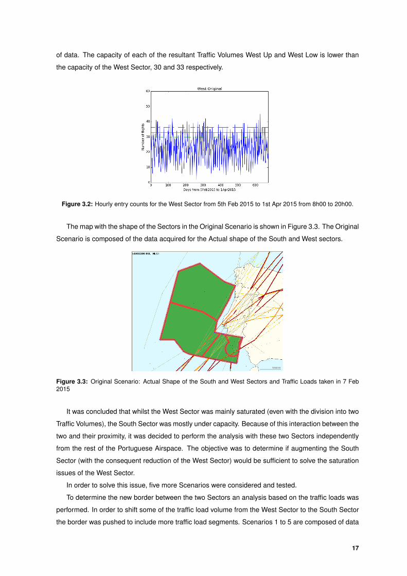
of data. The capacity of each of the resultant Traffic Volumes West Up and West Low is lower than

the capacity of the West Sector, 30 and 33 respectively.

Figure 3.2: Hourly entry counts for the West Sector from 5th Feb 2015 to 1st Apr 2015 from 8h00 to 20h00.

The map with the shape of the Sectors in the Original Scenario is shown in Figure 3.3. The Original

Scenario is composed of the data acquired for the Actual shape of the South and West sectors.

Figure 3.3: Original Scenario: Actual Shape of the South and West Sectors and Traffic Loads taken in 7 Feb2015

It was concluded that whilst the West Sector was mainly saturated (even with the division into two

Traffic Volumes), the South Sector was mostly under capacity. Because of this interaction between the

two and their proximity, it was decided to perform the analysis with these two Sectors independently

from the rest of the Portuguese Airspace. The objective was to determine if augmenting the South

Sector (with the consequent reduction of the West Sector) would be sufficient to solve the saturation

issues of the West Sector.

In order to solve this issue, five more Scenarios were considered and tested.

To determine the new border between the two Sectors an analysis based on the traffic loads was

performed. In order to shift some of the traffic load volume from the West Sector to the South Sector

the border was pushed to include more traffic load segments. Scenarios 1 to 5 are composed of data

17

acquired with the redefinition of the shape of both sectors.

The Scenarios considered are shown in Figures 3.4 to 3.6.

Figure 3.4: Scenario 1 (left) and 2 (right): Shape of the South and part of the West Sectors and Traffic Loadstaken in 7 Feb 2015.

Figure 3.5: Scenario 3 (left) and 4 (right): Shape of the South and part of the West Sectors and Traffic Loadstaken in 28 Feb 2015.

Figure 3.6: Scenario 5: Shape of the South and part of the West Sectors and Traffic Loads taken in 28 Feb2015.

In the new Scenarios created, the West Sector was not divided.

18

3.2 Numerical Optimization

3.2.1 Cost Function

In order to build the algorithm to calculate the cost of each scenario, the following steps were

required.

3.2.1.A Data Transformation

Firstly the data needed to describe the optimization problem was gathered from the tool NEST pre-

viously mentioned. The points of the frontiers of each sector and the points of the flight’s trajectories

of 2 AIRAC files were acquired.

Concerning the data extracted from the sectors, as explained in Section 2.1.1, these are divided

into airblocks. Therefore, the points extracted from the tool are relevant to the airblocks and each

sector has n airblocks.

The obstacle early on in this section was in the difference in precision between the data from the

flight points and from the airblock points. This difference resulted in an impossibility to test equality

between points and in intersections. The solutions to this problem will be explained in detail in the

subsections when found necessary.

To later perform the optimization, it was important to make sure that the points that were shared by

more than one sector changed together; i.e., it had to be made a correspondence between points in

common so that if one point in a given airblock changed, and that point was shared by other airblocks,

it would also be changeg in those airblocks. This prevented the creation of empty areas in between

sectors.

3.2.1.B Reduction of Sector Points

In the Optimization using Polygonal Sectors, the points in the frontiers of the sectors are the

variables to be optimized since these points define the shape of the sectors and the objective is to

find their optimal configuration.

The time necessary for the optimization process to complete depends heavily on the number of

variables to be optimized. Due to this, the number of points needed to be shortened.

The first method used to perform this reduction was based in the difference in slopes of two

consecutive airblock lines. If the difference in slopes of a line composed of two consecutive airblock

points and the following line was lower than a Threshold (α), then they represented the same line. In

this case, the middle point could be deleted from the sector.

The threshold (α) was given in degrees and represented the maximum accepted difference in

angle from the two lines.

The second method used was the Split and Merge, explained in 2.3.3.

19

3.2.1.C Create Box

The first step taken towards calculating the intersections between the flights and the airblocks

segments was to find in which airblock the flight points were in.

Firstly a box was created around each airblock with the maximum and minimum longitude and

latitude. Each point in each flight was tested for each airblock in each sector. The points were tested

against the box; if the box was missed so was the polygon.

If the coordinates of the point were inside the box created around the airblock, the point could be

inside the same. The point was saved along with the identification of the airblock.

If however the coordinates of the point were outside the box then the point was certainly outside

the airblock and the next airblock was tested. If the point missed all the boxes, then it was outside of

the Portuguese Airspace and was discarded.

The output was therefore a list of possible airblocks for each point.

3.2.1.D Inside Sectors

The points obtained in 3.2.1.C were then used to calculate the exact airblock in which each point

was in.

The algorithm used is described in 2.3.1.

The nuance for the algorithm presented is in the previously described difference in precision be-

tween the flight and the airblock points particularly when testing for special cases. Because of the

difference in precision, when calculating an intersection point (in special cases a) and b) described in

2.3.1) although the result should be exactly coincident with the vertex of the polygon, this would not

happen. This resulted in an impossibility to execute the algorithm proposed.

The solution to this problem was to add a Threshold (∆) so that an intersection point would be

considered the same as the previously found if they were closer than ∆. This is shown in Equation 3.1

where xintrs is the intersection point found in the current iteration and xbefore the previously found. If

the result from this equation was True, then the two points would be considered equal and the rest of

the algorithm would be executed.

xintrs ∈ [xbefore −∆;xbefore + ∆] (3.1)

To compare the intersection points found and check if it was equal to the maximum or minimum

in each segment, the same would be done. The point would be considered equal to the maximum or

minimum of the segment if they were closer than ∆.

The ∆ used was 1e− 10, chosen to be the minimum precision between the two sets of points.

3.2.1.E Calculation of the Time of Intersection

The algorithm created to calculate the times of intersection for each flight in the airblocks it crossed

is presented in Algorithm 3.1, where a is the current airblock; aentrance andmentrance are the airblock of

20

entrance and the segment of the airblock of entrance; R is the list containing the times of intersections

found; and A contains the previously entered and exited airblocks.

If a flight trajectory point is inside a given airblock, the intersection is tested for the segment

between that point and the point before by (T,M) = calc intrs(f [i0 − 1], f [i0], a). If the function

returns only one time of intersection, it will represent the time of entrance or exit of the airblock

analyzed, depending on the time of entrance being previously determined or not.

If the function returns more than one time of intersection, then it may occur that the segment it

is considering is the same as the segment of entrance. In that case all the segments in the result

are analyzed and the time of exit is equal to the time of intersection of segment m in M where

m 6= mentrance.

Special cases covered by the algorithm presented:

• Intersection with the following point - If the airblock and the flight segment changed but it was not

calculated an exit time, then the intersection between the last point analyzed and the following

with the entrance airblock is computed. This is necessary because the following point may not

be inside the entrance airblock and if the intersection is not calculated between the last and the

following an exit time will not be found. This will only be tested if the previous airblock was the

entrance airblock.

• Previously entered airblock - If the airblock considered was entered before, the current point is

saved and the search for another entrance airblock is continued. If there is a saved point and the

segments of entrance are not the same as the exit segments saved in R for the same airblock

then the intersection is tested. This is necessary so that the same intersection is not tested

twice and therefore the flight does not enter the airblock it had just left. To perform this, if the

segments of entrance in the airblock calculated were the same as the segments of exit in the

same airblock, then the intersection calculated was the exit intersection. All other possibilities

are tested for the same flight segment and only if it does not enter any other airblock it will be

considered it is entering the same airblock again.

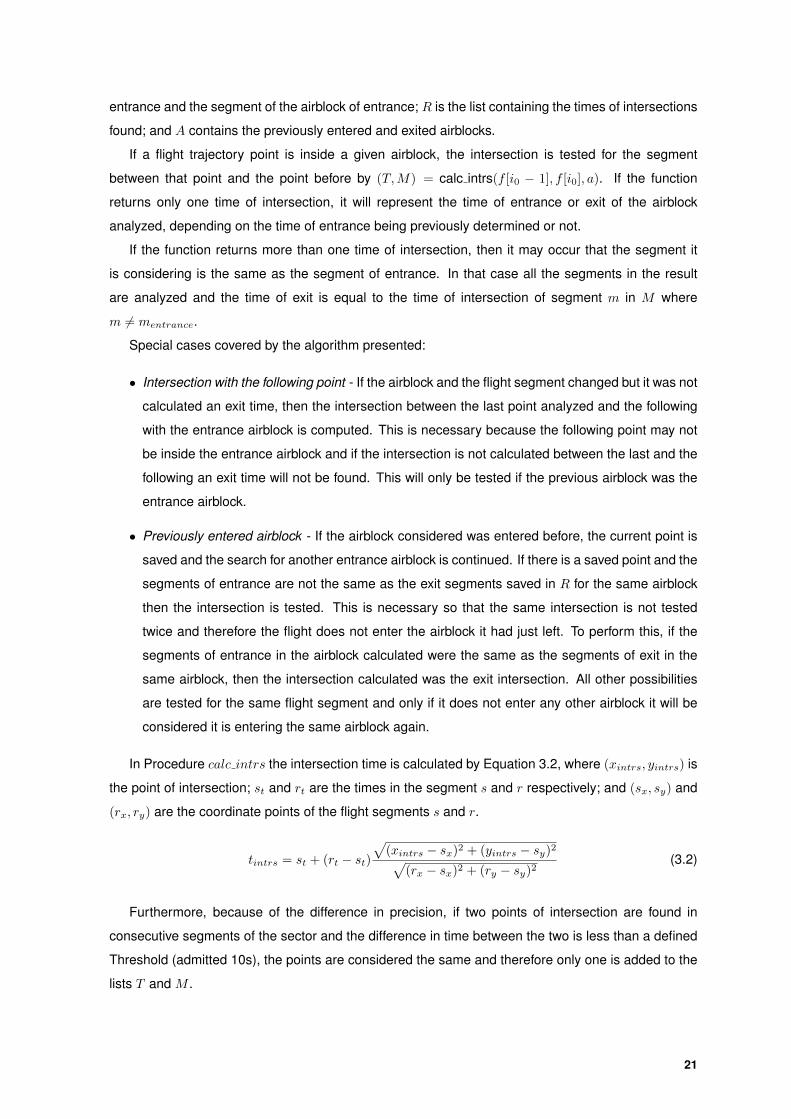
In Procedure calc intrs the intersection time is calculated by Equation 3.2, where (xintrs, yintrs) is

the point of intersection; st and rt are the times in the segment s and r respectively; and (sx, sy) and

(rx, ry) are the coordinate points of the flight segments s and r.

tintrs = st + (rt − st)√

(xintrs − sx)2 + (yintrs − sy)2√(rx − sx)2 + (ry − sy)2

(3.2)

Furthermore, because of the difference in precision, if two points of intersection are found in

consecutive segments of the sector and the difference in time between the two is less than a defined

Threshold (admitted 10s), the points are considered the same and therefore only one is added to the

lists T and M .

21

Algorithm 3.1 Calculation of the Time of Intersection

1: procedure CALC TIME(F ,S, I)2: Input: F - List of flights3: S - List of Sectors and respective airblocks4: I - List containing for each flight in F a list of points and the sectors they are in5: Each i in I has the format: i = (number of the entry in F , sector, airblock)6: Initial: Set R and A as empty lists7:8: for each f in F do9: for each i in I respecting f do

10: a = (i1, i2)11:12: if a 6= abef and i0 6= segm prev and an exit time has not been calculated then13: texit = calc intrs(f [ibef 0], f [ibef 0 + 1], aent)14: R← (aentrance, tentrance, texit)15: A← aentrance16: Reset aentrance17: if a ∈ A then18: Save variables a and i and continue to the next point in I19: if there is a point saved and there has not been calculated an entrance time then20: if the segment of entrance is not the same as the last exit segment then21: tentrance = calc intrs(f [isaved0

− 1], f [isaved0], asaved)

22: Reset asaved23:24: (T,M) = calc intrs(f [i0 − 1], f [i0], a)25: if len(T ) = 1 then26: if there has not been found an entrance time then27: tentrance = T28: aentrance = a29: mentrance = M30: else31: texit = T32: A← (aentrance, tentrance, texit)33: Reset aentrance34: A← a35: if len(T ) > 1 then36: for m in M do37: if m 6= mentrance then38: texit = t in T corresponding to m39: R← (aentrance, tentrance, texit)40: Reset aentrance41: A← a42: abef = a43: segm prev = i044: Reset abef , segm prev,A

return R45:46: procedure CALC INTRS(s, r, a)47: Input: s - Entry in F , r - Entry after s in F , a - Airblock48: Initial: Set T,M as empty lists49:50: for each segment in a do51: if a point of intersection (xintrs, yints) is found then52: Calculate tintrs and mintrs

53: T ← tintrs and M ← mintrs

return T,M

22

Multiple Sectors Test

One circumstance that was not described in Algorithm 3.1 but was implemented was the entrance

in multiple sectors.

If the entrance time in an airblock (B) is not the same as the exit time of the previous airblock (A)

then the flight has crossed airblocks in between the two airblocks found.

In that case, an additional point is created in the middle of the segment that entered and exited

the airblocks B and A respectively. This additional point is tested to see in which airblock it may be in.

If the generated point is inside an airblock (C) different from A and B, then an intersection with the

airblock C is tested and the times of entrance and exit are saved.

If however, the point is in airblock B, then a new point is created between the last point and the

point inside airblock A (closer to airblock A). Equation 3.3 shows the calculation of the new point,

where Point1 is the point inside airblock A; Point2 is the point inside airblock B; and m decreases

with the number of iterations. It starts with the value m = 1 and is divided by two with each iteration

(so that the new point is generated closer than the last to Point1). The opposite happens if the point

is inside airblock A, in which case the new point is created closer to airblock B.

NewPoint = Point1 +mPoint2 − Point1

4(3.3)

The point is tested again. New points are created until the new point is inside an airblock different

from A and B, or until a limit of divisions is reached (m = 164 ).

The time of entrance and exit is given in seconds of the day.

3.2.1.F Cost Calculation

The result obtained from 3.2.1.E is the time of entrance and exit for each airblock each flight

crossed. To calculate the output cost what is required is the time of entrance and exit in each sector.

Since each airblock identification contained the sector identification, the time of entrance in a

sector was the time of entrance in the first airblock contained in the specific sector and the time of exit

of the sector was determined as the time of exit from the last airblock belonging to the same sector

for each flight.

This information was then used to count the number of flights per sector per hour period. The time

frame used in the analysis was from 8h00 - 20h00.

The parameter chosen to determine the cost of each scenario was a weighted deviation between

the values of maximum capacity in each sector and the values of occupancy in each hour period.

The cost per sector j per day i is then given by Equation 3.4, where wijm is the weight attributed

to the time period m of sector j in day i ; countijm the occupancy of sector j in day i in the time period

m determined previously; and Cj is the value of maximum capacity for sector j (taken from the tool

NEST).

23

Vij =

#hours∑m=1

wijm(countijm−Cj)2

#hours∑m=1

wijm

, if countijm > Cj

#hours∑m=1

wijm(countijm−0.8Cj)2

#hours∑m=1

wijm

, otherwise

(3.4)

The weights were assigned as shown in Equation 3.5, so that the cost would be zero if the occu-

pancy of a sector was between 80% and 100% of the capacity of that sector.

wijm =

10, if countijm > Cj

0, if 0.8Cj < countijm < Cj

1, otherwise(3.5)

The global cost per sector j is the average of costs per day given in Equation 3.6.

Vj =

#days∑i=1

Vij

#days(3.6)

The final cost is an average of all the sectors given in Equation 3.7.

V =

#sectors∑i=1

Vj

#sectors(3.7)

The value of the cost function for each sector in a given time period (Vijm) is shown in Figure 3.7.

0.0 0.2 0.4 0.6 0.8 1.0 1.2 1.4Hourly entry count / Capacity

0.0

0.5

1.0

1.5

2.0

2.5

Cost Function

Figure 3.7: Cost Function.

3.2.2 Optimization using Polygonal Sectors

The first Optimization implemented consisted in performing changes to the current configuration

of sectors in the attempt to find a local minimum where the changes were not too drastic compared

to the Original Scenario. The thought behind this implementation was then to achieve a solution that

did not differ much from the Original setting so that few changes had to be made. This was important

24

because of the amount of resources needed to invest to educate controllers in the use of the new

Scenarios. This implementation was therefore a temporary fix to the problem.

In order to achieve this, the points that were in common between the outer sectors of the airspace

considered and the frontier of the same were fixed. The only points that could change were the

points inside the border so that the border was maintained. The number of points and their connec-

tions remained the same throughout the optimization and consequently the number of airblocks and

sectors.

Twist Condition: To avoid the lines that compose the sector to twist, and therefore split the sector

into two, the Interior Point Method explained in 2.4.3 was implemented. Whenever the lines crossed

and a twist was produced, the cost function would rise artiffically by the addition of a term dependent

on the distance of the knot created to the closest limit of the sector, giving a rough estimation of how

much the points had to move until the knot was eliminated.

The optimization method used was Differential Evolution, introduced in Section 2.4.2.

3.2.3 Optimization using Voronoi Diagrams

The second Optimization performed consisted in the creation of Voronoi regions, explained in

2.3.4, to represent the shape of the sectors. The optimization consisted in finding the best coordinates

for the generator points in order to reduce the cost calculated; the sectorization problem was simplified

to finding generating points.

The Voronoi Diagram was then constructed with the coordinates of the generator points obtained.

In order to translate this information into sectors, intersections between the regions formed and the

border of the airspace considered were calculated. To perform this, the frontier of the airspace had to

be determined resorting to the points of the airblocks.

The resulting sectors were defined as the area in each Voronoi region that was inside the frontier.

The algorithm to perform this intersection and construction is presented in Algorithm 3.2, where the

vertices of the Voronoi Diagram (C) are the points that constitute the segments around each generator

point; and Sectors contains as many entrances as the number of generating points.

The first vertex corresponding to each generating point iss tested to determine whether or not

it is inside Lisbon FIR, and the variable out is set accordingly to the result obtained. The test is

accomplished using PIP. If the vertex is inside the area, then it is added to the sector in Sectors

corresponding to p - Sectorsp.

Afterwards, for each segment in the Voronoi Diagram corresponding to the point p being tested,

intersections with each segment in the frontier are calculated. Any intersection found is saved.

If no intersection is found and the vertex is inside the FIR, then the point is added to the sector

points.

If only one intersection is found and the vertex is outside the FIR, two cases may occur. If the list

Sectorsp has not been filled yet, the point of intersection is added to the list. If however, the list is

not empty, then the sector must be filled with points from the frontier from the point previously found

and added to the list, to the current point found. The direction through which this closure is performed

25

Algorithm 3.2 Construction of sectors from Voronoi Diagram

1: procedure FRONTIER INTRS(F ,S,P, C,V)2: Input: F - List of frontier points3: S - List of frontier segments4: P - Set of Generating Points5: C - List with Voronoi vertices6: V - List with Voronoi segments7:8: Initial: Set I and Sectors as empty lists9:

10: for each p in P do11: Determine if the first vertex in P is inside the area defined by the frontier12: if the vertex is outside the area then13: out = 114: else15: out = 016: for each c in C respecting p do17: for each v in V respecting p do18: for each s in S do19: Calculate intersection between v and s20: if intersection i is found then21: I ← i22: Save variable s23: if len(I) = 0 and out = 0 then24: Sectorsp ← v

25: if len(I) = 1 and out = 1 then26: if Sectorsp is empty then27: Sectorsp ← i28: else29: if dist(F [s], p) < dist(F [s], t ∈ P\{p}) then30: Close the sector with points from the frontier counterclockwise31: else32: Close the sector with points from the frontier clockwise33: out = 034: if len(I) = 1 and out = 0 then35: Sectorsp ← i36: segmexit = s37: out = 138: if len(I) = 2 and out = 1 then39: Insert both i (in I) in Sectorsp40: if Sectorsp0

6= Sectorsplastthen

41: Close the sector with points from the frontier42: return Sectors43: procedure DIST(a, b)44: d =

√(xb − xa)2 + (yb − ya)2

45:46: return d

26

(clockwise or counterclockwise) defines the shape of the sector. The distance between one of the

points that form the segment of intersection s - Point s in S - and the generating points are tested.

For a point to be considered inside a Voronoi Region, it must be closer to the generating point of that

region than to any other generating point, as explained in Section 2.3.4. The points from the frontier

are defined counterclockwise in the vector F . Due to this, if the distance from point s to the generating

point p is smaller than the distance from s to any other p in P, then the sector must be closed with the

points from the frontier taken counterclockwise from the last segment of intersection saved (segmexit)

to s. If the opposite happens, then the sector must be closed with the points from the frontier taken

clockwise from segmexit to s. Since the vertex was outside the FIR and one intersection was found,

then the next vertex will be outside the FIR, and the variable out is set to zero.

If only one intersection is found and the vertex is inside the FIR, then the intersection point i in I

is added to the list Sectors. For the same reason than the one described in the previous case, the

variable out is set to one.

If two intersections with the frontier are found, it means both vertices are outside the frontier, and

both intersection points are added to the list Sectors.

Finally, if the first point in Sectors is not equal to the last point in the same list, then the sector

must be closed using points in the frontier. As occurred previously, the sector is closed with the points

belonging to the frontier that are closer to the generating point than the intersection points found.

In order to avoid the fragmentation of sectors, the Interior Point Method, explained in Section

2.4.3, was used. The distance from the segment formed and the point in the frontier furthest from this

segment was calculated to give an estimation of the distance the segment needed to move until the

sector was no longer fragmented. This distance would then be used to determine the term that was

added to the cost function. An example is shown in Figure 3.8, where one of the sectors is presented

fragmented and the furthest point from which to calculate the distance is shown as a red star.

A similar method was used in order to avoid the reduction of the number of sectors due to the

absence of intersections between a Voronoi region and the frontier of the airspace. In this last case,

instead of adding a term to the cost function, the cost function was assumed equal to the term and

was therefore dependent of the distance from the Voronoi segment that did not cross the frontier to

the frontier. This case is shown in Figure 3.9.

27

−20 −15 −10 −5Longitude

30

35

40

45

Lati

tude

Sector Fragmentation

Figure 3.8: Fragmentation of sectors - The blue dots represent the frontier of the FIR; the black lines the Voronoisegments created and the red star the furthest point from the segment that fragments the sector.

−20 −15 −10 −5Longitude

30

35

40

45

Lati

tude

Reduction of the number of sectors

Figure 3.9: Reduction of Sectors due to absence of intersections - The blue dots represent the frontier of theFIR; the black dots the generating points and the black lines the Voronoi segments created.

In order to calculate the cost, a measurement of the capacity of each sector formed was needed.

To perform this, the total capacity of the FIR was calculated as the sum of the capacities of each

original sector. The total area of the FIR was calculated through an application of the Green’s Theorem

explained in Section 2.3.5, where given the points that constitute the frontier the area of the same is

calculated. Finally, the total capacity is divided by the area previously determined, resulting in a

capacity per area. This capacity per area is later multiplied by the area of each sector obtained (also

calculated through Green’s Theorem) to give an estimate of the capacity of each sector.

28

This optimization resorting to Voronoi Diagrams allowed for a higher degree of freedom than

the previously shown optimization, as there were no restraints on points that needed to remain un-

changed.

29

30

4Results for the Preliminary Study

Contents4.1 Scenario 1 and Scenario 2 . . . . . . . . . . . . . . . . . . . . . . . . . . . . . . . . 324.2 Scenario 3 to Scenario 5 . . . . . . . . . . . . . . . . . . . . . . . . . . . . . . . . . 364.3 Scenario 1 and Scenario 2 with South Divided . . . . . . . . . . . . . . . . . . . . 38

31

In this chapter the results from the initial manual approach to the optimization problem will be

presented. In Section 4.1 it will be presented the initial results with the first two Scenarios created;

in Section 4.2 the results for the remaining Scenarios is presented; in Section 4.3 a final approach is

elaborated.

4.1 Scenario 1 and Scenario 2

The values corresponding to the actual daily entry count between 5th February 2015 and 1st April

2015 were acquired for the two new scenarios. The graphs computed from the data acquired of the

South and West Sectors are shown in Figures 4.1 and 4.2.

Figure 4.1: Scenario 1: Daily entry count from 5 Feb 2015 to 1 Apr 2015 from 8h00 to 20h00 for the South andWest Sectors.

Figure 4.2: Scenario 2: Daily entry count from 5 Feb 2015 to 1 Apr 2015 from 8h00 to 20h00 for the South andWest Sectors.

To better evaluate the performance of each Scenario and how they compare to one another, dif-

ferent criteria were chosen.

• Over Capacity: Average number of flights that exceed the sector’s capacity in the days it is

32

exceeded.

• Over 110: Average number of flights that exceed 110% of the sector’s capacity in the days it is

exceeded.

• Hours Over 110: Average number of hours per day in which the capacity is exceeded in more

than 110%.

• Hours Under 80: Average number of hours per day in which the sector is under 80% capacity.

• Under 80: Average volume of traffic that is untapped - Sum of the differences between 80%

Capacity and the number of flights in an hour period.

• Peak: Average of the daily maximum traffic.

• %Peak: Peak in relation to the Capacity

• Maximum Peak: Maximum Peak in the interval of days observed.

• %Maximum Peak: Maximum Peak in relation to the Capacity

• Days Saturated: Number of days in which the sector is saturated.

The %Peak criteria described above is obtained from Equation 4.1.

%Peak =Peak − Capacity

Capacity(4.1)

Two additional criteria were added to the above described: Deviation and Weighted Deviation.

The Deviation of a day is calculated from Equation 4.2, where xi is the traffic in each hour period

(from 8h00 to 20h00) of that day. The Deviation is a measure that is used to quantify the amount of

variation or dispersion of a set of data values. In this case the deviation is calculated from an ideal

value as opposed to the convencional standard deviation that uses the mean of the set of values. It

is assumed that the ideal value for the set of data is 90% the Capacity. Therefore, a Deviation close

to zero indicates that the data points tend to be close to the ideal value of the set, whereas a high

Deviation indicates that the data points are spread out over a wider range of values.

σ =

√N∑i=1

(xi − 0.9Capacity)2

N(4.2)

The Weighted Deviation of a day is obtained from Equation 4.3, where wi is defined in Equation

4.4 (where C is the capacity of each Sector). The Weighted Deviation, unlike the Deviation, allows

the attribution of different weights to different cases (In the Deviation the weight is always equal to

one). In this particular case, it allows the attribution of different weights to the cases where the Sector

is under 90% capacity and the cases where the Sector is over 110% capacity.

This is particularly helpful in this case taken into account it is more important to eliminate the over

saturation than it is to eliminate the lack of exploitation of the Sector.

33

σ =

√N∑i=1

wi(xi − 0.9Capacity)2

N∑i=1

wi

(4.3)

w[i][j][m] =

10, if xi > 1.1 ∗ C0, if 0.9 ∗ C < xi < 1.1 ∗ C1.5, if xi < 0.9 ∗ C

(4.4)

To calculate the final value of both the Deviation and the Weighted Deviation, an average was

made with the values obtained from each day in the time period considered.

The results calculated for the South Sector are shown in Table 4.1. The values shown were

calculated from data obtained from 5th Feb 2015 - 1st Apr 2015.

Table 4.1: South Sector: Comparison between Original Scenario, Scenario 1 and Scenario 2.

SOUTHOriginal Scenario 1 Scenario 2

Over Capacity (#Flights) 9.6 24.0 25.5Over 110 (#Flights) 3.9 17.3 16.9

Hours Over 110 0.2 0.7 0.9Hours Under 80 10.4 8.4 8.2

Under 80 (#Flights) 224.8 201.4 197.3Peak (#Flights) 34.5 40.5 40.9

%Peak -15.8 -1.3 -0.3Maximum Peak (#Flights) 51.0 60.0 61.0

%Maximum Peak 24.4 46.3 48.8Days Saturated 10 19 20

Deviation (#Flights) 15.3 12.4 12.1Weighted Deviation (#Flights) 15.4 13.3 13.1

The result for the West Sector is shown in Table 4.2.

Table 4.2: West Sector: Comparison between Original Scenario, Scenario 1 and Scenario 2.

WESTOriginal Scenario 1 Scenario 2




%Peak 7.1 -7.3 -13.5Maximum Peak (#Flights) 45.0 41.0 39.0



In order to achieve a single quantitative result that would be easier to use in order to compare the

different scenarios, a weighted average was made using the different criteria. Each value obtained

for each scenario was normalized with the values from the Original Scenario, following Equation 4.5,

34

where Vij is the value for Criteria i in Scenario j and ViO is the value for Criteria i in the Original

Scenario. Afterwards the values were multiplied by the respective weight of each criteria and divided

by the sum of weights.

Vij =Vij − VioViO

(4.5)

The weights for each criteria are depicted in Table 4.3.

Table 4.3: Weights for each Criteria

WeightsOver Capacity 2

Over 110 6Hours Over 110 1Hours Under 80 1

Under 80 1Peak 0

%Peak 2Maximum Peak 0

%Maximum Peak 2Days Saturated 0

Deviation 1Weighted Deviation 3

Table 4.4 contains the results for both Scenarios.

Table 4.4: Final Result for Scenarios 1 and 2

Scenario 1 Scenario 2Result South 29.68 30.47Result West -7.05 -9.64

The West Sector improved in comparison to the Original Scenario in both Scenarios. The average

number of flights over capacity and over 110% dropped as well as the average number of hours over

110%. The increase in both Deviations can be explained by the increase in unexploited volume of

traffic - As can be seen by criteria Under 80 and Hours Under 80, the West Sector presents worst

results than the Original Scenario because of the shift of traffic to the South Sector.

The South Sector however had an increase higher than the decrease in the West Sector in average

number of flights over capacity and over 110% as well as in number of days saturated (Mainly because

of the non division of the West Sector in Scenarios 1 and 2). The decrease in average number of hours

under 80% capacity and in the Under 80 criterion may be explained by the increase in traffic in the

Sector, which also results in lower values for both Deviations. However this decrease is not enough to

compensate the values obtained for the saturation, which can be observed by the high value in Table

4.4 in the comparison between the Original Scenario and Scenarios 1 and 2.

From the analysis of the data obtained it was clear that although the West Sector had improved

in comparison to the Original Scenario, the results in the South Sector were not satisfactory. The

improvements in the West Sector did not compensate the deterioration of the South Sector.

35

4.2 Scenario 3 to Scenario 5

Since the results obtained from the previous redefinition of the shape of both sectors in analysis

were worst than the results wanted, new Scenarios were created to try and solve the problem. Since

the problem with the previously created Scenarios was the over saturation of the South Sector, in the

new Scenarios a more gradual increase in the borders of the South Sector was aimed.

The results obtained for the daily saturation in the newly created Scenarios is shown in Figures

4.3 and 4.4.

Figure 4.3: Scenario 3 to 5: Daily entry count from 5 Feb 2015 to 1 Apr 2015 from 8h00 to 20h00 for the SouthSector.

36

Figure 4.4: Scenario 3 to 5: Daily entry count from 5 Feb 2015 to 1 Apr 2015 from 8h00 to 20h00 for the WestSector.

The combined results calculated for the criteria for the South Sector are shown in Table 4.5. The

values shown were calculated from data obtained from 5th Feb 2015 - 1st Apr 2015.

Table 4.5: South Sector: Comparison between Original Scenario and Scenarios 1 to 5.

SOUTHOriginal Scenario 1 Scenario 2 Scenario 3 Scenario 4 Scenario 5

Over Capacity (#Flights) 9.6 24.0 25.5 27.8 27.2 37.5Over 110 (#Flights) 3.9 17.3 16.9 13.2 13.3 20.4

Hours Over 110 0.2 0.7 0.9 0.3 0.3 0.4Hours Under 80 10.4 8.4 8.2 11.3 9.6 9.3

Under 80 (#Flights) 224.8 201.4 197.3 134.9 215.4 212.5Peak (#Flights) 34.5 40.5 40.9 36.4 36.8 38.2

%Peak -15.8 -1.3 -0.3 -11.3 -10.1 -6.9Maximum Peak (#Flights) 51.0 60.0 61.0 54.0 55.0 55.0

%Maximum Peak 24.4 46.3 48.8 31.7 34.1 39.0Days Saturated 10 19 20 15 14 17

Deviation (#Flights) 15.3 12.4 12.1 14.5 14.1 13.6Weighted Deviation (#Flights) 15.4 13.3 13.1 15.0 14.6 14.1

The results for the West Sector are shown in Table 4.6.

37

Table 4.6: West Sector: Comparison between Original Scenario and Scenarios 1 to 5.

WESTOriginal Scenario 1 Scenario 2 Scenario 3 Scenario 4 Scenario 5

Over Capacity (#Flights) 7.7 4.3 3.8 13.4 6.0 4.8Over 110 (#Flights) 5.0 2.7 2.0 8.9 4.8 8.4

Hours Over 110 0.6 0.1 0.1 1.3 0.4 0.2Hours Under 80 6.1 10.0 10.7 7.4 8.9 9.1

Under 80 (#Flights) 108.2 161.4 168.7 133.9 148.3 151.0Peak (#Flights) 34.2 30.6 28.5 38.2 33.2 32.5

%Peak 7.1 -7.3 -13.5 15.9 0.7 -1.5Maximum Peak (#Flights) 45.0 41.0 39.0 53.0 46.0 45.0

%Maximum Peak 50 24.2 18.2 60.6 39.4 36.4Days Saturated 35 14 9 45 28 26

Deviation (#Flights) 12.6 13.5 14.4 11.0 12.4 12.5Weighted Deviation (#Flights) 9.6 13.7 14.5 11.1 13.9 13.2

The final result is given by Table 4.7

Table 4.7: Final Result for Scenarios 1 to 5

Scenario 1 Scenario 2 Scenario 3 Scenario 4 Scenario 5Result South 29.68 30.47 16.58 17.17 34.54Result West -7.05 -9.64 22.72 -3.63 -8.25

As can be observed, in Scenario 3 the reduction of the West Sector was not enough to compensate

the non division of the same sector. In the days the West Sector suffered from the highest amount

of traffic, the vertical division of the sector allowed the traffic to spread over the two created sectors,

reducing saturation and therefore the peaks of traffic. Because of this division the Original Scenario

performed better than Scenario 3.

In Scenario 4 and 5 there is an improvement to the West Sector, although still worse than Scenar-

ios 1 and 2.

In the South Sector the results are still not satisfactory but Scenario 4 appears to be the one that

gives the best trade-off between the increase in traffic in the South Sector and the improvement of

the situation in the West Sector from the five Scenarios created. Nevertheless the West Sector in

the Original Scenario is not as saturated as the South Sector in Scenario 4, which may lead to the

conclusion that the Original Scenario performs better.

4.3 Scenario 1 and Scenario 2 with South Divided

The results from the Scenarios previously created were not achieving the intended because of the

impossibility to compensate the improvement in the West Sector with the deterioration of the South

Sector while shifting from three Sectors (South, West Up and West Low) to only two (South and West)

and having as only degree of freedom the movement of the border between them.

Since the results from Scenario 1 and 2 were satisfactory concerning the West Sector, it was

decided to perform a vertical division on the South Sector in the days over saturation occurred.

The first step taken was to find the optimal FL in which to perform the vertical division of the Sector.

To do so, results for the South Sector were obtained by dividing it into different FL and then compared

38

in order to determine the best division. The results for each FL were obtained by extracting data for

the two Sectors created (South Up and South Low) and performing calculations for both. In the days

South was over saturated and therefore divided, the value obtained for each criteria in the Upper part

of the Sector was compared with the value obtained for the same criteria in the Lower part. The worst

value between the two was the one chosen to be representative of that criteria in each specific day.

From this analysis the FL chosen was 355. The data obtained from this division is shown in Table

4.8 (The values for the West Sector remain the same as the previously calculated for the Scenarios 1

and 2, since the only Sector changed was the South Sector).

Table 4.8: South Sector Divided: Comparison between Original Scenario, Scenario 1 and Scenario 2.

SouthOriginal South Divided Scenario 1 South Divided Scenario 2




%Peak -15.8 -9.5 -8.8Maximum Peak (#Flights) 51.0 41.0 42.0



The values corresponding to the daily entry count between 5th February 2015 and 1st April 2015

are shown in Figure 4.5 and the final result is shown in Table 4.9.

Figure 4.5: Scenario 1 and 2 with South Divided: Daily entry count from 5 Feb 2015 to 1 Apr 2015 from 8h00 to20h00 for the Southt Sector.

Table 4.9: Final Result for Scenarios 1 and 2 with South Divided

South Divided Scenario 1 South Divided Scenario 2Result South -4.83 -3.72Result West -10.58 -12.43

39

As can be observed, the over capacity in both Scenarios was reduced in comparison to the Original

Scenario resulting in an average of three flights per day above the capacity in the days the capacity

was exceeded as opposed to the average of nine for the Original Scenario. In agreement with the

previous results, the average number of flights over 110% and the average number of hours where it

occurred also dropped.

Furthermore both Deviations dropped, which verifies the statement that the new Sectors present

a better distribution of traffic around the ideal value of 90% Capacity than the Original Scenario.

Based on these results, it is possible to state that this division is better than the Original Scenario

using the same amount of resources (Three Sectors).

Between Scenario 1 and 2 the results obtained from the South Sector are very similar. The values

for over capacity and for over 110% capacity are roughly the same; both Scenarios present an average

peak and maximum peak bellow the value from the Original Scenario (having an average peak bellow

capacity); and Scenario 2 has slightly better results in the criteria corresponding to the occupancy

bellow 80%.

40

5Results for the Numerical

Optimization

Contents5.1 Algorithm - Cost Function . . . . . . . . . . . . . . . . . . . . . . . . . . . . . . . . 425.2 Optimization using Polygonal Sectors . . . . . . . . . . . . . . . . . . . . . . . . . 455.3 Optimization using Voronoi Diagrams . . . . . . . . . . . . . . . . . . . . . . . . . 48

41

In this Chapter the results obtained will be presented and analyzed. In Section 5.1 the results from

the implementation of the Algorithm will be shown; In Section 5.2 the results from the first optimization

implemented will be presented; and in Section 5.3 the results from the optimization using Voronoi

Diagrams will be discussed.

5.1 Algorithm - Cost Function

In this Section, intermediate results from the implementation of the algorithm to calculate the

cost function for the optimization problem will be shown and explained. It will also be presented an

explanation for the need to introduce certain conditions for the algorithm to work, shown in 3.2.1.

5.1.1 Reduction of the Sector Points

As stated in 3.2.1.B, the number of points to be optimized has high influence in the time necessary

for the optimization to run. The number of points extracted from NEST to represent the sectors was

2602.

After the correspondence of points, the number of points was decreased to 568. As the border

was fixed and the respective points could not move, the number of points to be optimized was further

reduced to 384.

The results are shown in Table 5.1, where different Thresholds are used in the reduction method

implemented.

Table 5.1: Results for the Reduction of Sector Points.

# Points Border FixedInitial 2602

Correspondence 568Fixing Points in the Border 384

Difference of Slopesα = 1◦ 332α = 5◦ 314α = 10◦ 304

Figures 5.1 and 5.2 show the results of the reduction of points using the Difference of Slopes

method in a cut of the sectors in 365FL.

As can be seen, the number of points decreases with the increase in the Threshold (α). Most of

the redundant points in the outer frontier of the FIR are eliminated with the application of the algorithm

with α = 1◦. The scenario obtained for α = 5◦ is very similar to the scenario obtained for α = 10◦.

In the later, all the redundant points were eliminated while maintaining the shape of the frontier of the

FIR and the sectors border.

42

−18 −16 −14 −12 −10 −8 −6Longitude

32

34

36

38

40

42

Lati

tude

Original Scenario - FL365

Figure 5.1: Reduction of Sector Points - Original Scenario Cut in 365FL (Latitude and Longitude are degrees).

−18 −16 −14 −12 −10 −8 −6Longitude

32

34

36

38

40

42

Lati

tude

Threshold = 1

−18 −16 −14 −12 −10 −8 −6Longitude

32

34

36

38

40

42

Threshold = 5

−18 −16 −14 −12 −10 −8 −6Longitude

32

34

36

38

40

42

Threshold = 10

Figure 5.2: Reduction of Sector Points - Scenarios obtained for α = 1◦, 5◦ and 10◦ Cut in 365FL (Latitude andLongitude in degrees).

5.1.2 Multiple Sectors Test

In Figures 5.3 and 5.4 examples of the Multiple Sectors Test condition are shown. The sectors

shown in the following Figures are the sectors for which entrance and exit intersection times were

found and calculated.

43

−14 −12 −10 −8 −6 −4 −2Longitude

35

36

37

38

39

40

41

42

43

44

Lati

tude

Before

Sector (1, 11)Sector (1, 9)Sector (7, 5)Sector (4, 1)Sector (15, 1)

−14 −12 −10 −8 −6 −4 −2Longitude

35

36

37

38

39

40

41

42

43

44

Lati

tude

After

Sector (1, 11)Sector (1, 9)Sector (7, 5)Sector (4, 1)Sector (15, 1)Sector (1, 12)Sector (7, 2)

Figure 5.3: Multiple Sectors Test Condition - Intersections calculated by the algorithm before and after theintroduction of the condition (Intersections marked as red stars), example 1 - Latitude and Longitude in degrees.

−11 −10 −9 −8 −7 −6Longitude

36

37

38

39

40

41

42

Lati

tude

Before

Sector (10, 3)Sector (2, 9)Sector (2, 10)Sector (8, 7)Sector (8, 6)

−11 −10 −9 −8 −7 −6Longitude

36

37

38

39

40

41

42

Lati

tude

After

Sector (10, 3)Sector (2, 9)Sector (2, 10)Sector (8, 7)Sector (8, 6)Sector (8, 5)

Figure 5.4: Multiple Sectors Test Condition - Intersections calculated by the algorithm before and after theintroduction of the condition (Intersections marked as red stars), example 2 - Latitude and Longitude in degrees.

The black dots in both Figures represent the trajectory points for two different flights, taken from

real flight track data on 6th February 2015.

As can be seen from Figure 5.3, before the condition was implemented, because there were no

trajectory points inside Sectors (1,12) and (7,2), intersection times could not be calculated with these

sectors since there was no information on their existence between the two sectors calculated. But the

time of exit from Sector (1,9) and the time of entrance in Sector (7,5) were different.

With the implementation of the Multiple Sectors Test and consequently the addition of a point in

between the segment that created the exit and entrance intersections from Sectors (1,9) and (7,5)

respectively, it was possible to determine intersections with Sectors (1,12) and (7,2), as can be seen

from the after Scenario in Figure 5.3.

44

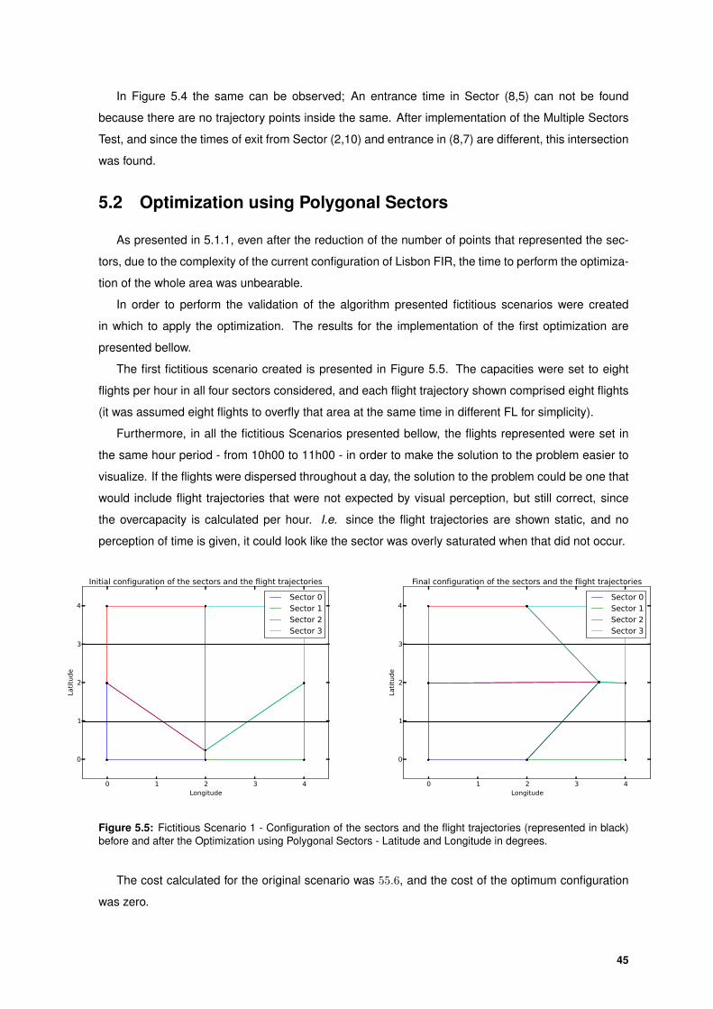
In Figure 5.4 the same can be observed; An entrance time in Sector (8,5) can not be found

because there are no trajectory points inside the same. After implementation of the Multiple Sectors

Test, and since the times of exit from Sector (2,10) and entrance in (8,7) are different, this intersection

was found.

5.2 Optimization using Polygonal Sectors

As presented in 5.1.1, even after the reduction of the number of points that represented the sec-

tors, due to the complexity of the current configuration of Lisbon FIR, the time to perform the optimiza-

tion of the whole area was unbearable.

In order to perform the validation of the algorithm presented fictitious scenarios were created

in which to apply the optimization. The results for the implementation of the first optimization are

presented bellow.

The first fictitious scenario created is presented in Figure 5.5. The capacities were set to eight

flights per hour in all four sectors considered, and each flight trajectory shown comprised eight flights

(it was assumed eight flights to overfly that area at the same time in different FL for simplicity).

Furthermore, in all the fictitious Scenarios presented bellow, the flights represented were set in

the same hour period - from 10h00 to 11h00 - in order to make the solution to the problem easier to

visualize. If the flights were dispersed throughout a day, the solution to the problem could be one that

would include flight trajectories that were not expected by visual perception, but still correct, since

the overcapacity is calculated per hour. I.e. since the flight trajectories are shown static, and no

perception of time is given, it could look like the sector was overly saturated when that did not occur.

0 1 2 3 4Longitude

0

1

2

3

4

Latitude

Initial configuration of the sectors and the flight trajectories

Sector 0Sector 1Sector 2Sector 3

0 1 2 3 4Longitude

0

1

2

3

4

Latitude

Final configuration of the sectors and the flight trajectories


Figure 5.5: Fictitious Scenario 1 - Configuration of the sectors and the flight trajectories (represented in black)before and after the Optimization using Polygonal Sectors - Latitude and Longitude in degrees.

The cost calculated for the original scenario was 55.6, and the cost of the optimum configuration

was zero.

45

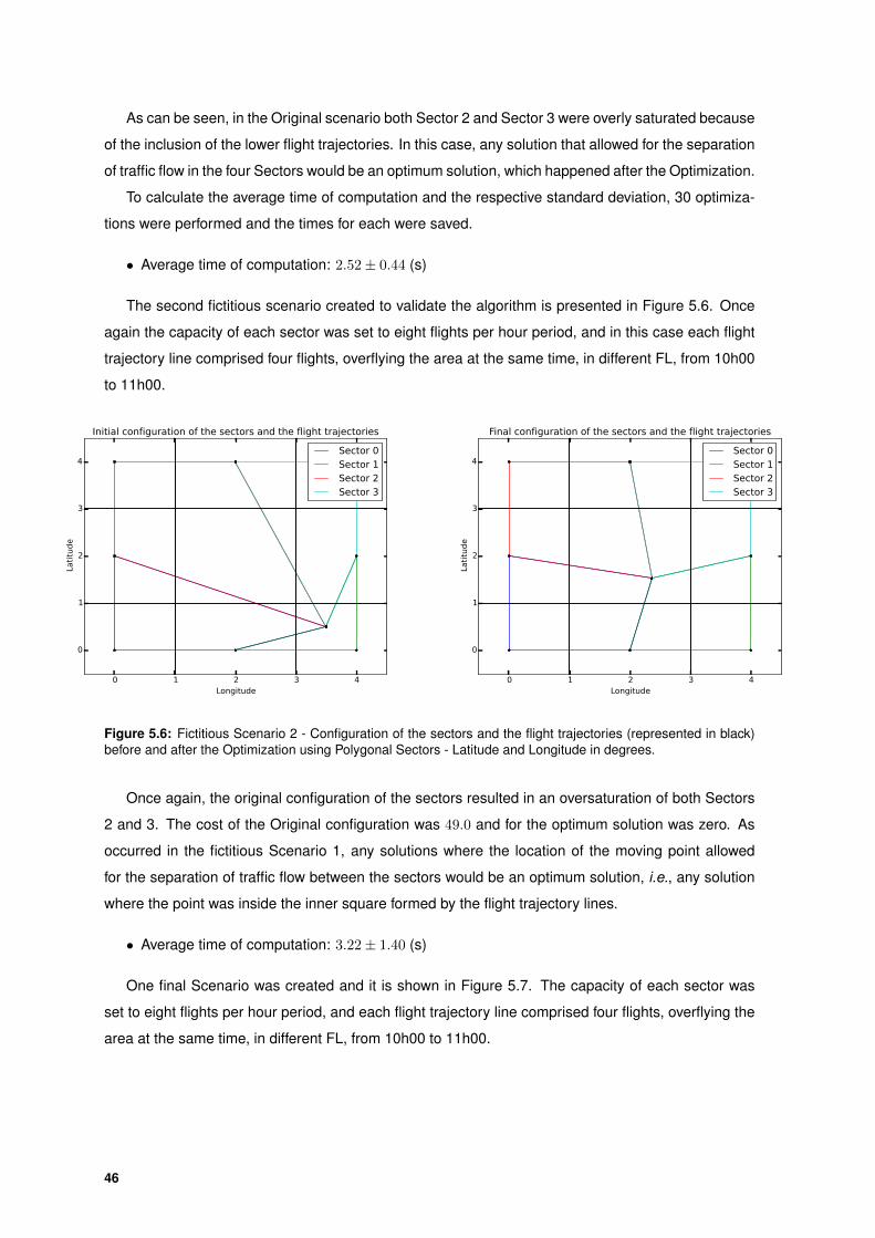
As can be seen, in the Original scenario both Sector 2 and Sector 3 were overly saturated because

of the inclusion of the lower flight trajectories. In this case, any solution that allowed for the separation

of traffic flow in the four Sectors would be an optimum solution, which happened after the Optimization.

To calculate the average time of computation and the respective standard deviation, 30 optimiza-

tions were performed and the times for each were saved.

• Average time of computation: 2.52± 0.44 (s)

The second fictitious scenario created to validate the algorithm is presented in Figure 5.6. Once

again the capacity of each sector was set to eight flights per hour period, and in this case each flight

trajectory line comprised four flights, overflying the area at the same time, in different FL, from 10h00

to 11h00.

0 1 2 3 4Longitude

0

1

2

3

4

Latitude



0 1 2 3 4Longitude

0

1

2

3

4La

titude




Once again, the original configuration of the sectors resulted in an oversaturation of both Sectors

2 and 3. The cost of the Original configuration was 49.0 and for the optimum solution was zero. As

occurred in the fictitious Scenario 1, any solutions where the location of the moving point allowed

for the separation of traffic flow between the sectors would be an optimum solution, i.e., any solution

where the point was inside the inner square formed by the flight trajectory lines.


One final Scenario was created and it is shown in Figure 5.7. The capacity of each sector was

set to eight flights per hour period, and each flight trajectory line comprised four flights, overflying the

area at the same time, in different FL, from 10h00 to 11h00.

46

0 1 2 3 4 5 6Longitude

0

1

2

3

4

5

6

Latitude



0

1

2

3

4

5

6

Latitude



The cost of the optimum solution found was zero, and 26.7 for the original configuration.

In this Scenario it is possible to see the influence of the condition implemented that the sectors

could not twist. In Figure 5.8 the result after the optimization without the implementation of the Twist

Condition is presented.


0

1

2

3

4

5

6

Latitude

Twist Condition

Figure 5.8: Fictitious Scenario 3 before the Twist Condition - Configuration of the sectors and the flight trajecto-ries (represented in black) after the Optimization using Polygonal Sectors - Latitude and Longitude in degrees.


Analysing the times of computation for the three scenarios presented, it is possible to observe that

all three scenarios have very high standard deviation in comparison to the average calculated. This

can be explained by the random nature of the optimization used - Differential Evolution. Since the

new values in each iteration are obtained by probability combination of the previous existing values,

there are higher differences in the times calculated for each run.

It can still be observed that the times are as high as it was expected. The first two scenarios had

only one point to be optimized and 16 flights in which to test the intersections. Both took around 3

seconds to compute. The third scenario had four points in the optimization and 24 flights, and the

average time needed to conclude the optimization was 177 seconds, almost 3 minutes. Considering

47

that for each day, more than 1000 flights overfly Lisbon FIR and the number of sector points in the

optimization was 304, it can be seen that with the resources available, the time it would need to

conclude the optimization was unbearable.

From the Design Constraints for the construction of sectors presented in Section 2.2, the con-

straints this implementation does not satisfy are the Convexity and the Boundary Constraint. The

Workload and the Connectivity Constraints are satisfied.

The Boundary and Convexity Constraint are not satisfied as the only constraint imposed to the

movement of points is the Twist Condition. No constraint is implemented to avoid acute angles and

therefore an aircraft may re-enter a sector it had just left; and no condition is imposed to the distance

between the points created and the waypoints.

The Connectivity Constraint is satisfied as the sector points maintain its connection throughout the

optimization and are not allowed to fragment.

The Workload Constraint is satisfied as the optimum solution searched is the one that presents

the minimum value of deviation from the value of capacity for each sector. Therefore the search is

always performed with the objective of not trespassing the limit for each sector, which complies with

the Workload Constraint.

5.3 Optimization using Voronoi Diagrams

The complexity of the sectors and hence the number of points in the representation via Voronoi Di-

agrams decreased significantly from the previous representation. In order to compute the optimization

of the Lisbon FIR using the previous optimization, about 300 points had to be optimized. To compute

the same number of sectors (17) in this optimization, only 17 points had to be used.

In order to compare the two algorithms, the optimization was also run for the fictiocious scenarios

presented previously.

The results for the first fictitious scenario are presented in Figure 5.9, where two solutions are

shown.

48

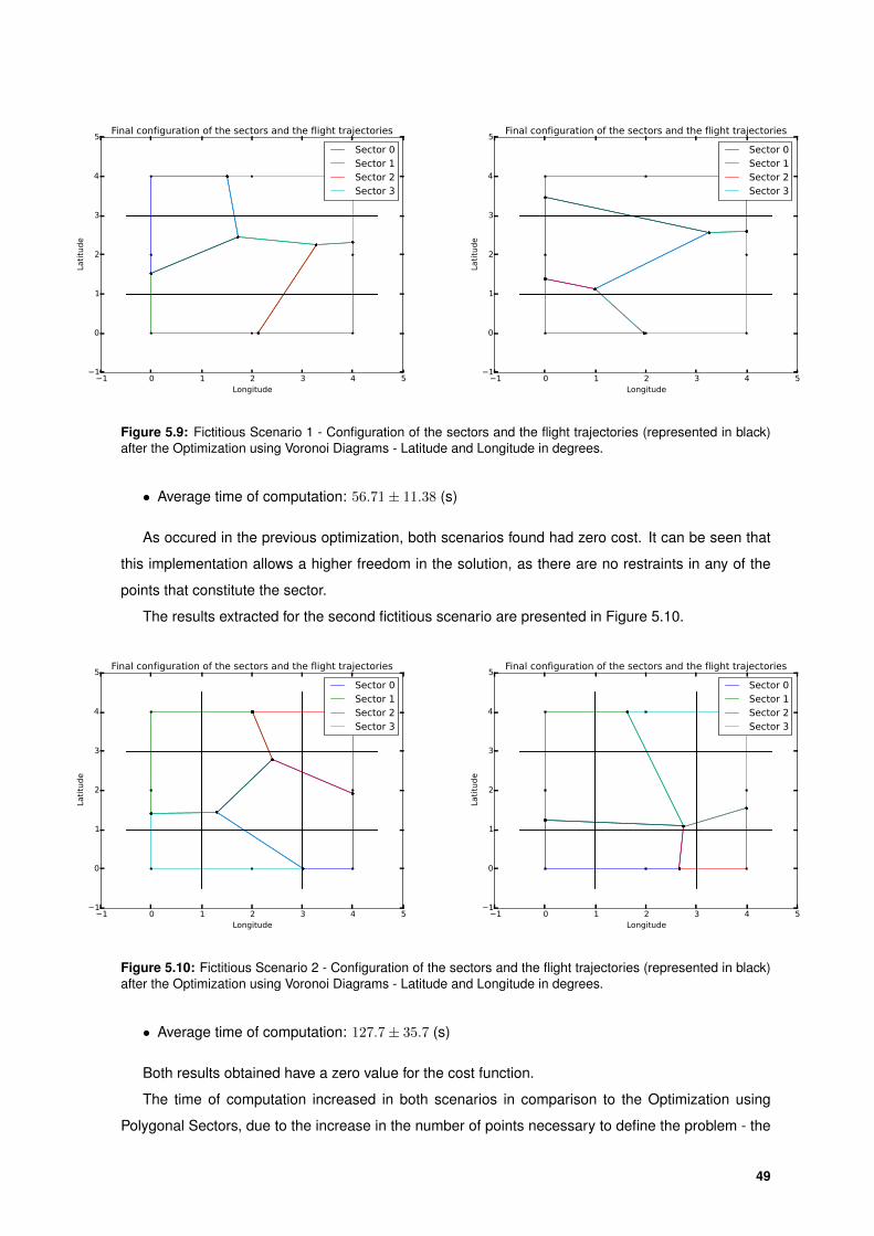
−1 0 1 2 3 4 5Longitude

−1

0

1

2

3

4

5

Lati

tude



−1 0 1 2 3 4 5Longitude

−1

0

1

2

3

4

5

Lati

tude



Figure 5.9: Fictitious Scenario 1 - Configuration of the sectors and the flight trajectories (represented in black)after the Optimization using Voronoi Diagrams - Latitude and Longitude in degrees.


As occured in the previous optimization, both scenarios found had zero cost. It can be seen that

this implementation allows a higher freedom in the solution, as there are no restraints in any of the

points that constitute the sector.

The results extracted for the second fictitious scenario are presented in Figure 5.10.

−1 0 1 2 3 4 5Longitude

−1

0

1

2

3

4

5

Lati

tude



−1 0 1 2 3 4 5Longitude

−1

0

1

2

3

4

5

Lati

tude





Both results obtained have a zero value for the cost function.

The time of computation increased in both scenarios in comparison to the Optimization using

Polygonal Sectors, due to the increase in the number of points necessary to define the problem - the

49

previous optimization only required one point, and this requires four. The advantages of this method

in terms of time can only be seen in a scenario that involves more complex sector shapes.

The results obtained for the third fictitious scenario are presented in Figure 5.11.

−1 0 1 2 3 4 5 6 7Longitude

−1

0

1

2

3

4

5

6

7

Lati

tude


Sector 0Sector 1Sector 2Sector 3Sector 4Sector 5Sector 6Sector 7Sector 8



As occured in the previous scenarios, the average time of computation was higher than the time

obtained in the Optimization using Polygonal Sectors. This can be explained by the augmentation in

number of points in the optimization - nine in this last optimization and four in the previous.

The advantage of this optimization is that the complexity of the scenarios created in terms of

sectors construction does not differ much from the complexity in Lisbon FIR, which does not occur

when polygonal sectors are used.

The time it would take to compute this optimization with 17 points can be roughly estimated by the

growth in time from the previous scenarios to this last one. Taking into account the number of points

necessary to construct the 17 sectors using polygonal sectors, and performing the same estimation

with the data obtained for this optimization, it is possible to conclude that although the first optimization

method had a better performance in terms of time in the scenarios created, as the problem is scaled,

the second optimization method will present better results.

From the Design Constraints for the construction of sectors presented in Section 2.2, the only

constraint this optimization does not satisfy is the Boundary Constraint. The Workload, the Convexity

and the Connectivity Constraints are satisfied.

The Boundary Constraint is not satisfied as there is no condition imposed for the distance of the

points in the border of the sectors and possible points of conflict and waypoints.

Since each region of the Voronoi Diagram are obtained from the intersection of half-spaces, and

hence are convex polygons, the Convexity Constraint is satisfied.

The Connectivity Constraint is satisfied because of the inclusion of the condition that sectors can

50

not be fragmented, explained in Section 3.2.3.

As in the former optimization, the Workload Constraint is satisfied as the cost function is calculated

based on the difference between the hourly count and the capacity for each sector.

51

52

6Conclusions and Future Work

Contents6.1 Conclusions . . . . . . . . . . . . . . . . . . . . . . . . . . . . . . . . . . . . . . . . 546.2 Future Work . . . . . . . . . . . . . . . . . . . . . . . . . . . . . . . . . . . . . . . . 55

53

The concluding remarks of this thesis and recommendations for future work are presented in this

chapter.

6.1 Conclusions

The work developed in this thesis concerned the search for an optimal partition of the portuguese

airspace. To reach the intended outcome, algorithms to successfully calculate daily entry counts for

real traffic data and to define the shape of the intended sectors were derived. The main conclusions

that can be drawn from this thesis are the following:

• In an initial preliminary approach to the problem, the over saturation in the South and West

Sectors of the Lisbon FIR was studied and resolved. The solution found to this problem was in

compliance with the NAV requests and concerns of future traffic evolution.

• Algorithms were created to reduce the number of points that represented the sectors, in order to

reduce the complexity of the problem. The size of the problem was successfully reduced from

an initial state involving 568 points (after the correspondence of the points in common) to 304

points with the application of the method suggested with α = 10◦.

• An algorithm was implemented in order to calculate times of entrance and exit in the sectors

created. The algorithm was tested in the original scenario of Lisbon FIR and the times were

validated with the times specified by NEST. The algorithm successfully calculated entrance

and exit times for each flight trajectory in all the sectors of the original scenario it crossed.

This validated the use of the algorithm created to calculate daily entry counts in the scenarios

subsequently created.

• In order to validate the Optimization using Polygonal Sectors, three fictitious scenarios were

created. The scenarios proposed were simple in order for the solution to be obvious. The

optimization was applied to the three scenarios, and in all of them an optimal solution was found,

with zero cost. The times of computation were as high as expected. Also as expected, this

method presented several limitations. It served the purpose for which it had been constructed

- as a temporary fix to the current problem, allowing for the sectors not to change drastically

in relation to the original partitioning of the airspace. But it did not guarantee that the solution

found was the best in terms of workload distribution.

• The Optimization using Voronoi Diagrams was then implemented in order to have a method

that had no limitation on choosing costs and was able to simultaneously balance the workload,

maintain the preferred shape, and optimize given costs.

• An algorithm was constructed to create Voronoi Diagrams from any set of generating points,

and to find the area that resulted from its intersection with a closed frontier. This algorithm was

tested for several different scenarios, with frontiers ranging from simple geometric shapes to the

frontier of Lisbon FIR, and the algorithm performed as expected.

54

• In order to validate the Optimization using Voronoi Diagrams, the optimization was performed in

the two first scenarios used previously. This optimization allowed a higher degree of freedom in

the solutions found, and it satisfied the Convexity Constraint, that the previous did not. Besides

the convex sector shapes, the major advantage of using the Voronoi Diagrams was detaching

the graph partition and optimization. The goal of the problem became finding optimal generating

points that minimize the cost, as opposed to optimal frontier points, which reduced the size of

the problem.

• Due to lack of resources, the application of both optimizations in Lisbon FIR was not possible.

The algorithms were created and tested for the implementation in this area, but no results were

possible to be extracted. Since both optimizations behaved well in the scenarios presented, it

can be concluded that the problem can be scaled and the algorithms can be used to solve the

initial problem.

6.2 Future Work

The following topics are relevant for future work in research of the optimum sectorization of the

Portuguese airspace:

• Convexity Constraint in the Optimization using Polygonal Sectors. One of the constraints this

optimization does not satisfy is the convexity constraint. It would be possible to incorporate it by

adding a condition that did not allow acute angles to form between consecutive sector segments,

and applying interior point methods to add a term dependent on the angle to the cost function.

• Boundary Constraint on both Optimizations. Neither one of the optimizations satisfy the Bound-

ary Constraint. A way to achieve this would be to form a list with the possible points of conflict

and waypoints, and add a condition that stated that no point in the border of the sector could be

closer to these points by more than a determined distance.

• Design Constraints. The design constraints proposed in this thesis are only a portion of the

design constraints provided by ICAO. For the sake of simplification of the problem, these con-

straints were considered the most important and were the only analyzed, but the incorporation

of the rest of the constraints would be of interest in order to obtain a solution closer to one that

can be implemented in a real Scenario.

• Split and Merge. The algorithm Split and Merge was studied and implemented, but it was not

possible to extract results. The time this method would require to compute would be higher than

the time needed for the method shown, but it would be compensated by the reduction of points

and therefore time needed for the optimization.

• Duplication of points. In the optimization using polygonal sectors, the immobilization of points in

the frontier of the FIR reduces the degrees of freedom of the problem and restricts the optimal

solution. To solve this issue, it would be possible to duplicate the points in common between the

55

outer sectors and the border of Lisbon FIR, so that they could also change. This would allow for

the frontier between the sectors to change while maintaining the outer shape of the airspace.

• Calculation of the capacity. In the division of the airspace using Voronoi Diagrams, the estima-

tion of the capacity of the sectors generated is a rought estimation. A better estimation would

be possible using the DORATASK method about sector capacity evaluation by British operations

research and analysis council. This method states that the whole workload of controllers can be

divided in to two parts. One part is visible control work time that can be measured under normal

conditions or when flight conflicts occur, such as the time for delivering ATC clearances, listen-

ing to captain read back, coordinating handoff and filling out strips. The other part is invisible

control work time that cannot be measured, such as the time for observing airspace status and

thinking about control plans. The use of this method would increase the level of reliability in the

results obtained.

• Addition of height in Optimization using Voronoi Diagrams. In the Optimization using Voronoi

Diagrams, the problem is solved only in 2D. The sectors are considered only to change in latitude

and longitude and remain constant in height. It would add complexity and improve the results

if the height was added as an extra variable in the optimization, as it would allow, among other

situations, for the sectors to split.

• Weight in the Cost Function. The cost function proposed in this thesis for the Numerical Op-

timization had a plateau in zero when all the sectors presented entry counts between 80 and

100% the capacity of each sector. This cost function does not prevent some unbalances be-

tween sectors, as some sectors may reach 100% capacity - and therefore be at the edge of over

saturation, and others just above 80% - and still be able to sustain more traffic. Furthermore, the

optimal area was too wide - The number of solutions with cost equal to zero was too high. One

alternative would be to assign a small weight to the cases where the calculated entry count was

between 80% and 100% capacity.

56

Bibliography

[1] J.-R. Sack and J. Urrutia, Handbook of computational geometry. Elsevier, 1999.

[2] “Challenges of Growth 2013,” EUROCONTROL, Bruxelles, Belgium, Tech. Rep., June 2013.

[3] S.-C. Han and M. Zhang, “The optimization method of the sector partition based on metamorphic

voronoi polygon,” Chinese Journal of Aeronautics, vol. 17, no. 1, pp. 7–12, 2004.

[4] D. Delahaye, M. Schoenauer, and J.-M. Alliot, “Airspace sectoring by evolutionary computation,”

Spatial evolutionary modelling, pp. 203–233, 2001.

[5] J. S. Mitchell, G. Sabhnani, J. Krozel, B. Hoffman, A. Yousefi, and P. Kopardekar, “Dynamic

airspace configuration management based on computational geometry techniques,” in AIAA

guidance, navigation, and control conference, 2008.

[6] S. Martinez, G. B. Chatterji, D. Sun, and A. M. Bayen, “A weighted-graph approach for dynamic

airspace configuration,” in Proceedings of the AIAA Conference on Guidance, Navigation, and

Control (GNC). American Institute of Aeronautics and Astronautics, 2007.

[7] D. Delahaye, “Optimisation de la sectorisation de l’espace aerien par algorithmes genetiques,”

Ph.D. dissertation, 1995.

[8] M. Xue, “Airspace sector redesign based on voronoi diagrams,” Journal of Aerospace Computing,

Information, and Communication, vol. 6, no. 12, pp. 624–634, 2009.

[9] “NEST - Network Strategic Tool,” EUROCONTROL, Bruxelles, Belgium, Tech. Rep., April 2015.

[10] T. Huy, P. Baptiste, and V. Duong, “Optimized sectorization of airspace with constraints,” in 5th

US/Europe ATM Seminar, Budapest, Hungary, 2003.

[11] S. Kulkarni, R. Ganesan, and L. Sherry, “Static sectorization approach to dynamic airspace con-

figuration using approximate dynamic programming,” in Integrated Communications, Navigation

and Surveilance Conference (ICNS), 2011. IEEE, 2011, pp. J2–1.

[12] S. Y. J Zhang, “Speeding up Large-Scale Point-in-Polygon Test Based Spatial Join on GPUs,”

2012.

[13] E. Haine, “Graphics gems IV,” in Point in Polygon Strategies, P. S. Heckbert, Ed. San Diego:

Academic Press, 1994.

57

[14] G. Taylor, “Point in Polygon Test,” Department of Surveying, University of Newcastle upon Tyne,

1994.

[15] V. Nguyen, A. Martinelli, N. Tomatis, and R. Siegwart, “A comparison of line extraction algo-

rithms using 2d laser rangefinder for indoor mobile robotics,” in Intelligent Robots and Systems,

2005.(IROS 2005). 2005 IEEE/RSJ International Conference on. IEEE, 2005, pp. 1929–1934.

[16] E. W. Weisstein, “Voronoi Diagram,” http://mathworld.wolfram.com/VoronoiDiagram.html, Octo-

ber 2015.

[17] F. Aurenhammer, “Voronoi diagrams - a survey of a fundamental geometric data structure,” ACM

Computing Surveys (CSUR), vol. 23, no. 3, pp. 345–405, 1991.

[18] A. Okabe, B. Boots, K. Sugihara, and S. N. Chiu, Spatial Tessellations: Concepts and Applica-

tions of Voronoi Diagrams. John Wiley & Sons, 2009, vol. 501.

[19] K. Price, R. M. Storn, and J. A. Lampinen, Differential evolution: a practical approach to global

optimization. Springer Science & Business Media, 2006.

[20] R. Storn and K. Price, Differential evolution-a simple and efficient adaptive scheme for global

optimization over continuous spaces. ICSI Berkeley, 1995, vol. 3.

[21] K. Price and R. Storn, “Differential evolution - a simple and efficient heuristic for global opti-

mization over continuous spaces,” Journal of global optimization, vol. 11, no. 4, pp. 341 – 359,

1997.

[22] R. Storn, “On the usage of differential evolution for function optimization,” in Fuzzy Information

Processing Society, 1996. NAFIPS., 1996 Biennial Conference of the North American. IEEE,

1996, pp. 519–523.

[23] A. Forsgren, P. E. Gill, and M. H. Wright, “Interior methods for nonlinear optimization,” SIAM

review, vol. 44, no. 4, pp. 525–597, 2002.

[24] S. Granville, “Optimal reactive dispatch through interior point methods,” Power Systems, IEEE

Transactions on, vol. 9, no. 1, pp. 136–146, 1994.

58

http://mathworld.wolfram.com/VoronoiDiagram.html

optimization of airspace sectorization in atm - … · optimization of airspace sectorization in...

Documents