optimal stock selling based on the global maximum · 6th world congress of the bachelier finance...
TRANSCRIPT

Optimal Stock Selling Based on the Global
Maximum
Yifei Zhong
University of Oxford
6th World Congress of the Bachelier Finance Society, June 22-26,2010
(joint work with Dr. M. Dai and Z. Yang)

If I were an Innocent Investor...
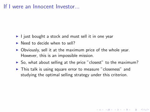
I just bought a stock and must sell it in one year
Need to decide when to sell?
Obviously, sell it at the maximum price of the whole year.However, this is an impossible mission.
So, what about selling at the price ”closest” to the maximum?
If I were an Innocent Investor...
I just bought a stock and must sell it in one year
Need to decide when to sell?
Obviously, sell it at the maximum price of the whole year.However, this is an impossible mission.
So, what about selling at the price ”closest” to the maximum?
This talk is using square error to measure ”closeness” andstudying the optimal selling strategy under this criterion.
The Model
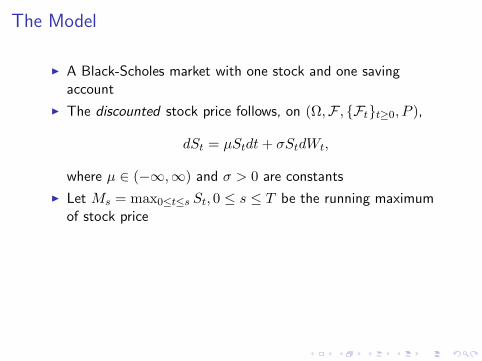
A Black-Scholes market with one stock and one savingaccount
The discounted stock price follows, on (Ω,F , Ftt≥0, P ),
dSt = µStdt+ σStdWt,
where µ ∈ (−∞,∞) and σ > 0 are constants
Let Ms = max0≤t≤s St, 0 ≤ s ≤ T be the running maximumof stock price

The Model
A Black-Scholes market with one stock and one savingaccount
The discounted stock price follows, on (Ω,F , Ftt≥0, P ),
dSt = µStdt+ σStdWt,
where µ ∈ (−∞,∞) and σ > 0 are constants
Let Ms = max0≤t≤s St, 0 ≤ s ≤ T be the running maximumof stock price
Consider the following optimal stopping problem
inf0≤ν≤T
E[(Sν −MT )2],
where E stands for the expectation, ν is an Ft-stopping time.
Related (Probabilistic) Literature
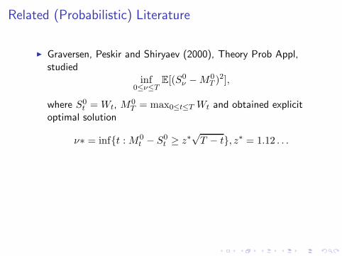
Graversen, Peskir and Shiryaev (2000), Theory Prob Appl,studied
inf0≤ν≤T
E[(S0ν −M0
T )2],
where S0t =Wt, M
0T = max0≤t≤T Wt and obtained explicit
optimal solution
ν∗ = inft :M0t − S0
t ≥ z∗√T − t, z∗ = 1.12 . . .

Related (Probabilistic) Literature
Graversen, Peskir and Shiryaev (2000), Theory Prob Appl,studied
inf0≤ν≤T
E[(S0ν −M0
T )2],
where S0t =Wt, M
0T = max0≤t≤T Wt and obtained explicit
optimal solution
ν∗ = inft :M0t − S0
t ≥ z∗√T − t, z∗ = 1.12 . . .
du Toit and Peskir (2007), Ann Prob, considered
inf0≤ν≤T
E[(Sµν −MµT )
2],
where µ 6= 0.

Related (Financial) Literature
Shiryaev, Xu and Zhou (2008), Quant Fin, studied the relativeerror between the selling price and global maximum,
inf0≤ν≤T
E
[
SνMT
]
”Bang-bang” strategy:
Sell at time T : µ > σ2
2
Sell at time 0 : µ ≤ σ2
2

PDE Formulation
The problem isinf
0≤ν≤TE[(Sν −MT )
2]
Not a standard optimal stopping problem, since MT is notFt-adapted
One more step:
inf0≤ν≤T
E[(Sν −MT )2] = inf
0≤ν≤TE
E[(Sν −MT )2 | Fν ]
= inf0≤ν≤T
E
φ(ν, Sν ,Mν)
,
where φ(t, St,Mt) = E[(St −MT )2 | Ft]
PDE Formulation (Con’t)
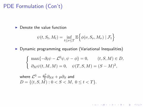
Denote the value function
ψ(t, St,Mt) = inft≤ν≤T
E
φ(ν, Sν ,Mν) | Ft
Dynamic programming equation (Variational Inequalities)
max−∂tψ − L0ψ,ψ − φ = 0, (t, S,M) ∈ D,
∂Mψ(t,M,M) = 0, ψ(T, S,M) = (S −M)2,
where L0 = σ2
2 ∂SS + µ∂S andD = (t, S,M) : 0 < S < M, 0 ≤ t < T.

The Obstacle Function φ(t, S,M)
Recall
φ(t, St,Mt) = E[(St −MT )2 | Ft]
= S2t − 2StE[MT | Ft] + E[M2
T | Ft]=: S2
t − 2Stφ1(t, St,Mt) + φ2(t, St,Mt),
where φi(t, St,Mt) = E[M iT | Ft].
Then, φi(t, S,M) satisfies
−∂tφi − L0φi = 0, (t, S,M) ∈ D,
∂Mφi(t,M,M) = 0, φi(T, S,M) =M i.

Change of Variables
Denote τ = T − t, x = ln MS, ui(τ, x) =
φi(t,S,M)Si ,
u(τ, x) = φ(t,S,M)S2 .
Then, u1 and u2 satisfy
∂τu1 − L1xu1 = 0 in Ω,
∂xu1(τ, 0) = 0, u1(0, x) = ex,
∂τu2 − L2xu2 = 0 in Ω,
∂xu2(τ, 0) = 0, u2(0, x) = e2x,
where L1x = σ2
2 ∂xx −(
µ+ σ2
2
)
∂x + µ,
L2x = σ2
2 ∂xx −(
µ+ 3σ2
2
)
∂x + (2µ + σ2),
Ω = (0, T ]× (0,∞).

Change of Variables (con’t)
Denote v(τ, x) = ψ(t,S,M)−φ(t,S,M)S2
Then, v satisfies
max
∂τv − L2xv −H, v
= 0 in Ω,
∂xv(τ, 0) = 0, v(0, x) = 0,
where H = L2xu− ∂τu = 2µ+ σ2 +2
(
σ2∂xu1 − (µ+ σ2)u1
)
,
L2x = σ2
2 ∂xx −(
µ+ 3σ2
2
)
∂x + (2µ + σ2).
Define the selling region (the stopping region) as follows:
SR = (τ, x) ∈ [0,∞) × (0, T ] : v(τ, x) = 0.

The Optimal Selling Strategy: Good Stock(µ > 0)
0 0.2 0.4 0.6 0.8 10
0.2
0.4
0.6
0.8
1
τ
x=
log
M S
x1s* (τ)
x2s* (τ)
SR
Figure: Two optimal selling boundaries. Parameter values used:µ = 0.045, σ = 0.3, T = 1.

The Optimal Selling Strategy: Bad Stock (−σ2 ≤ µ ≤ 0)
0 0.2 0.4 0.6 0.8 10
0.2
0.4
0.6
τ
x=
log
M S
SR
xs*(τ)
Figure: The monotonically increasing optimal selling boundary.Parameter values used: µ = −0.010, σ = 0.3, T = 1.

The Optimal Selling Strategy: Very Bad Stock (µ < −σ2)
0 0.5 1 1.5 2 2.5 30
0.04
0.08
0.12
0.16
τ
x=
log
M S
SRx
s*(τ)
Figure: The nonmonotone optimal selling boundary. Parameter valuesused: µ = −0.032, σ = 0.4, T = 3.

The Proof
Recall
max
∂τv − L2xv −H, v
= 0 in Ω,
∂xv(τ, 0) = 0, v(0, x) = 0,
So,
SR = (τ, x) : v = 0⊆ (τ, x) : ∂τ0− L2
x0−H ≤ 0= (τ, x) : H ≥ 0

The Set (τ, x) : H ≥ 0
Lemma: Recall H(τ, x) = 2µ+ σ2 + 2(
σ2∂xu1 − (µ+ σ2)u1
)
.
If µ ≤ 0, ∂xH > 0;
If µ ≥ −σ2, ∂τH < 0;
If µ > 0, ∂xH(τ, x) = 0 has at most one solution for any giveτ > 0;
-
6
•O
τ
x
γ
H < 0 H > 0
case µ ≤ 0
-
6
•O
•ln(
σ2
2µ + 1)
•τH
τ
x
γ1 γ2M
H > 0
H < 0
case µ > 0

The Main Results: µ ≤ 0
With the help of previous lemma, we have
∂xv ≥ 0 if µ ≤ 0;
∂τv ≤ 0 if µ ≥ −σ2;
These are due to
∂τv −L2xv = H, in (τ, x) : v < 0.

The Main Results: µ ≤ 0
With the help of previous lemma, we have
∂xv ≥ 0 if µ ≤ 0;
∂τv ≤ 0 if µ ≥ −σ2;
These are due to
∂τv −L2xv = H, in (τ, x) : v < 0.
Define x∗s(τ) = infx ∈ (0,+∞) : v(τ, x) = 0,∀τ ∈ (0, T ].
The Main Results: µ ≤ 0
With the help of previous lemma, we have
∂xv ≥ 0 if µ ≤ 0;
∂τv ≤ 0 if µ ≥ −σ2;
These are due to
∂τv −L2xv = H, in (τ, x) : v < 0.
Define x∗s(τ) = infx ∈ (0,+∞) : v(τ, x) = 0,∀τ ∈ (0, T ]. Thanks to ∂xv ≥ 0, we can show
SR = (τ, x) : v(τ, x) = 0= (τ, x) : x ≥ x∗s(τ), 0 < τ ≤ T.
∂τv ≤ 0 gives the monotonicity of the free boundary.
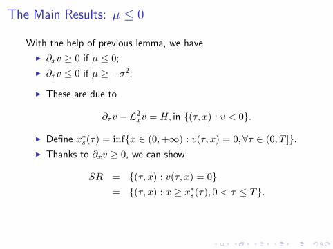
The Main Results: µ > 0
With µ > 0, we have ∂τv ≤ 0, which implies that(τ2, x) ∈ SR, if (τ1, x) ∈ SR and τ2 < τ1.
0 0.5 1 1.50
0.2
0.4
0.6
0.8
1
1.2
1.4
1.6
1.8
2
τ
x
H<0
H>0
(τ1,x
1)∈ SR
(τ1,x
2)∈ SR

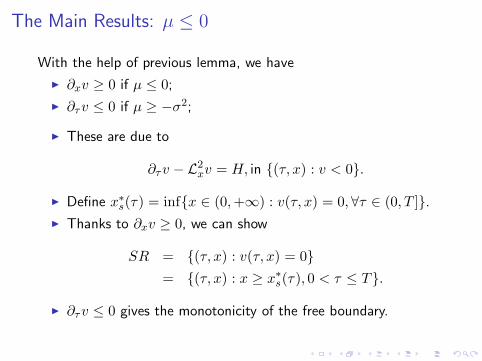
The Main Results: µ > 0
With µ > 0, we have ∂τv ≤ 0, which implies that(τ2, x) ∈ SR, if (τ1, x) ∈ SR and τ2 < τ1.
0 0.5 1 1.50
0.2
0.4
0.6
0.8
1
1.2
1.4
1.6
1.8
2
τ
x
H<0
(τ1,x
2)∈ SRv=0
(τ1,x
1)∈ SRv=0
H>0

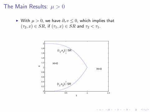
The Main Results: µ > 0
With µ > 0, we have ∂τv ≤ 0, which implies that(τ2, x) ∈ SR, if (τ1, x) ∈ SR and τ2 < τ1.
0 0.5 1 1.50
0.2
0.4
0.6
0.8
1
1.2
1.4
1.6
1.8
2
τ
x
H<0
(τ1,x
2)∈ SR
vτ−Lxv=H>0
v=0
(τ1,x
1)∈ SRv=0
H>0
Suppose v<0
v>0
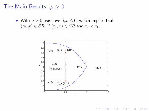
The Main Results: µ > 0
With µ > 0, we have ∂τv ≤ 0, which implies that(τ2, x) ∈ SR, if (τ1, x) ∈ SR and τ2 < τ1.
0 0.5 1 1.50
0.2
0.4
0.6
0.8
1
1.2
1.4
1.6
1.8
2
τ
x
H<0
(τ1,x
2)∈ SRv=0
H>0
v=0
v=0
(τ1,x
1)∈ SR
(τ,x)∈ SR

The Main Results: µ > 0
The sell region SR is connected;
We can define
x∗1s(τ) = infx ∈ [ 0,+∞) : v(τ, x) = 0x∗2s(τ) = supx ∈ [ 0,+∞) : v(τ, x) = 0
It is easy to show
SR = (τ, x) : x∗1s(τ) ≤ x ≤ x∗2s(τ), 0 < τ ≤ τ∗.
The monotonicity of x∗is(τ) follows by ∂τv ≤ 0.

Smoothness of the Free Boundary
For µ ≥ −σ2, we have ∂τv ≤ 0. So, one can easily establishthe smoothness of x∗s(τ) following Friedman (1975).
First, show x∗s(τ) ∈ C3/4((0, T ]) Then, show x∗s(τ) ∈ C1((0, T ]) By a bootstrap argument, show x∗s(τ) ∈ C∞((0, T ])

Smoothness of the Free Boundary
For µ ≥ −σ2, we have ∂τv ≤ 0. So, one can easily establishthe smoothness of x∗s(τ) following Friedman (1975).
First, show x∗s(τ) ∈ C3/4((0, T ]) Then, show x∗s(τ) ∈ C1((0, T ]) By a bootstrap argument, show x∗s(τ) ∈ C∞((0, T ])
For µ < −σ2, we change of variables. Let y = x− µ/σ2τ ,and V (τ, y) = v(τ, x).
Show ∂τV (τ, y) ≤ 0 and ∂yV (τ, y) ≥ 0 Apply Friedman (1975) to show smoothness of the
corresponding y∗s (τ), which gives the desired result
Conclusion
We examine the optimal decision to sell a stock with thecriteria of minimizing the square error between the sellingprice and the global maximum.
For good stock, i.e. µ > 0, the optimal selling boundary hastwo branches and only exists when time to maturity is notlong enough.
For bad stock, i.e. µ ≤ 0, the optimal selling boundary onlyhas one branch and always exists.
The smoothness of the free boundary is also established.

Thank you !