optimal rates of convergence for covariance matrix estimation · key words and phrases. covariance...
TRANSCRIPT

arX
iv:1
010.
3866
v1 [
mat
h.ST
] 1
9 O
ct 2
010
The Annals of Statistics
2010, Vol. 38, No. 4, 2118–2144DOI: 10.1214/09-AOS752c© Institute of Mathematical Statistics, 2010
OPTIMAL RATES OF CONVERGENCE FOR COVARIANCE
MATRIX ESTIMATION
By T. Tony Cai1, Cun-Hui Zhang2 and Harrison H. Zhou3
University of Pennsylvania, Rutgers University and Yale University
Covariance matrix plays a central role in multivariate statisticalanalysis. Significant advances have been made recently on developingboth theory and methodology for estimating large covariance matri-ces. However, a minimax theory has yet been developed. In this paperwe establish the optimal rates of convergence for estimating the co-variance matrix under both the operator norm and Frobenius norm.It is shown that optimal procedures under the two norms are differ-ent and consequently matrix estimation under the operator norm isfundamentally different from vector estimation. The minimax upperbound is obtained by constructing a special class of tapering estima-tors and by studying their risk properties. A key step in obtaining theoptimal rate of convergence is the derivation of the minimax lowerbound. The technical analysis requires new ideas that are quite dif-ferent from those used in the more conventional function/sequenceestimation problems.
1. Introduction. Suppose we observe independent and identically dis-tributed p-variate random variables X1, . . . ,Xn with covariance matrix Σp×p
and the goal is to estimate the unknown matrix Σp×p based on the sam-ple {Xi : i= 1, . . . , n}. This covariance matrix estimation problem is of fun-damental importance in multivariate analysis. A wide range of statisticalmethodologies, including clustering analysis, principal component analysis,linear and quadratic discriminant analysis, regression analysis, require theestimation of the covariance matrices. With dramatic advances in technol-ogy, large high-dimensional data are now routinely collected in scientificinvestigations. Examples include climate studies, gene expression arrays,
Received October 2008; revised September 2009.1Supported in part by NSF Grant DMS-06-04954.2Supported in part by NSF Grants DMS-05-04387 and DMS-06-04571.3Supported in part by NSF Career Award DMS-06-45676.AMS 2000 subject classifications. Primary 62H12; secondary 62F12, 62G09.Key words and phrases. Covariance matrix, Frobenius norm, minimax lower bound, op-
erator norm, optimal rate of convergence, tapering.
This is an electronic reprint of the original article published by theInstitute of Mathematical Statistics in The Annals of Statistics,2010, Vol. 38, No. 4, 2118–2144. This reprint differs from the original inpagination and typographic detail.
1

2 T. T. CAI, C.-H. ZHANG AND H. H. ZHOU
functional magnetic resonance imaging, risk management and portfolio al-location and web search problems. In such settings, the standard and mostnatural estimator, the sample covariance matrix, often performs poorly. See,for example, Muirhead (1987), Johnstone (2001), Bickel and Levina (2008a,2008b) and Fan, Fan and Lv (2008).
Regularization methods, originally developed in nonparametric functionestimation, have recently been applied to estimate large covariance matrices.These include banding method in Wu and Pourahmadi (2009) and Bickeland Levina (2008a), tapering in Furrer and Bengtsson (2007), thresholdingin Bickel and Levina (2008b) and El Karoui (2008), penalized estimation inHuang et al. (2006), Lam and Fan (2007) and Rothman et al. (2008), regu-larizing principal components in Johnstone and Lu (2009) and Zou, Hastieand Tibshirani (2006). Asymptotic properties and convergence results havebeen given in several papers. In particular, Bickel and Levina (2008a, 2008b),El Karoui (2008) and Lam and Fan (2007) showed consistency of their es-timators in operator norm and even obtained explicit rates of convergence.However, it is not clear whether any of these rates of convergence are opti-mal.
Despite recent progress on covariance matrix estimation there has beenremarkably little fundamental theoretical study on optimal estimation. Inthis paper, we establish the optimal rate of convergence for estimating thecovariance matrix as well as its inverse over a wide range of classes of covari-ance matrices. Both the operator norm and Frobenius norm are considered.It is shown that optimal procedures for these two norms are different andconsequently matrix estimation under the operator norm is fundamentallydifferent from vector estimation. In addition, the results also imply that thebanding estimator given in Bickel and Levina (2008a) is sub-optimal underthe operator norm and the performance can be significantly improved.
We begin by considering optimal estimation of the covariance matrixΣ over a class of matrices that has been considered in Bickel and Lev-ina (2008a). Both minimax lower and upper bounds are derived. We writean ≍ bn if there are positive constants c and C independent of n such thatc ≤ an/bn ≤ C. For a matrix A its operator norm is defined as ‖A‖ =sup‖x‖2=1 ‖Ax‖2. We assume that p ≤ exp(γn) for some constant γ > 0.Combining the results given in Section 3, we have the following optimalrate of convergence for estimating the covariance matrix under the operatornorm.
Theorem 1. The minimax risk of estimating the covariance matrix Σover the class Pα given in (3) satisfies
infΣ
supPα
E‖Σ−Σ‖2 ≍min
{
n−2α/(2α+1) +log p
n,p
n
}
.(1)

COVARIANCE MATRIX ESTIMATION 3
The minimax upper bound is obtained by constructing a class of taper-ing estimators and by studying their risk properties. It is shown that theestimator with the optimal choice of the tapering parameter attains theoptimal rate of convergence. In comparison to some existing methods inthe literature, the proposed procedure does not attempt to estimate eachrow/column optimally as a vector. In fact, our procedure does not opti-mally trade bias and variance for each row/column. As a vector estimator,it has larger variance than squared bias for each row/column. In other words,it is undersmoothed as a vector.
A key step in obtaining the optimal rate of convergence is the derivation ofthe minimax lower bound. The lower bound is established by using a testingargument, where at the core is a novel construction of a collection of leastfavorable multivariate normal distributions and the application of Assouad’slemma and Le Cam’s method. The technical analysis requires ideas that arequite different from those used in the more conventional function/sequenceestimation problems.
In addition to the asymptotic analysis, we also carry out a small simu-lation study to investigate the finite sample performance of the proposedestimator. The tapering estimator is easy to implement. The numerical per-formance of the estimator is compared with that of the banding estimatorintroduced in Bickel and Levina (2008a). The simulation study shows thatthe proposed estimator has good numerical performance; it nearly uniformlyoutperforms the banding estimator.
The paper is organized as follows. In Section 2, after basic notation anddefinitions are introduced, we propose a tapering procedure for the covari-ance matrix estimation. Section 3 derives the optimal rate of convergencefor estimation under the operator norm. The upper bound is obtained bystudying the properties of the tapering estimators and the minimax lowerbound is obtained by a testing argument. Section 4 considers optimal esti-mation under the Frobenius norm. The problem of estimating the inverseof a covariance matrix is treated in Section 5. Section 6 investigates the nu-merical performance of our procedure by a simulation study. The technicalproofs of auxiliary lemmas are given in Section 7.
2. Methodology. In this section we will introduce a tapering procedurefor estimating the covariance matrix Σp×p based on a random sample of p-variate observations X1, . . . ,Xn. The properties of the tapering estimatorsunder the operator norm and Frobenius norm are then studied and used toestablish the minimax upper bounds in Sections 3 and 4.
Given a random sample {X1, . . . ,Xn} from a population with covariancematrix Σ= Σp×p, the sample covariance matrix is
1
n− 1
n∑
l=1
(Xl − X)(Xl − X)T ,
4 T. T. CAI, C.-H. ZHANG AND H. H. ZHOU
which is an unbiased estimate of Σ, and the maximum likelihood estimatorof Σ is
Σ∗ = (σ∗ij)1≤i,j≤p =1
n
n∑
l=1
(Xl − X)(Xl − X)T ,(2)
when Xl’s are normally distributed. These two estimators are close to eachother for large n. We shall construct estimators of the covariance matrix Σby tapering the maximum likelihood estimator Σ∗.
Following Bickel and Levina (2008a) we consider estimating the covariancematrix Σp×p = (σij)1≤i,j≤p over the following parameter space:
Fα =Fα(M0,M) =
{
Σ:maxj
∑
i
{|σij | : |i− j|> k} ≤Mk−α
(3)
for all k, and λmax(Σ)≤M0
}
,
where λmax(Σ) is the maximum eigenvalue of the matrix Σ, and α> 0,M > 0and M0 > 0. Note that the smallest eigenvalue of any covariance matrix inthe parameter space Fα is allowed to be 0 which is more general than theassumption in (5) of Bickel and Levina (2008a). The parameter α in (3),which essentially specifies the rate of decay for the covariances σij as theymove away from the diagonal, can be viewed as an analog of the smooth-ness parameter in nonparametric function estimation problems. The optimalrate of convergence for estimating Σ over the parameter space Fα(M0,M)critically depends on the value of α. Our estimators of the covariance ma-trix Σ are constructed by tapering the maximum likelihood estimator (2) asfollows.
Estimation procedure. For a given even integer k with 1 ≤ k ≤ p, wedefine a tapering estimator as
Σ = Σk = (wijσ∗ij)p×p,(4)
where σ∗ij are the entries in the maximum likelihood estimator Σ∗ and theweights
wij = k−1h {(k − |i− j|)+ − (kh − |i− j|)+},(5)
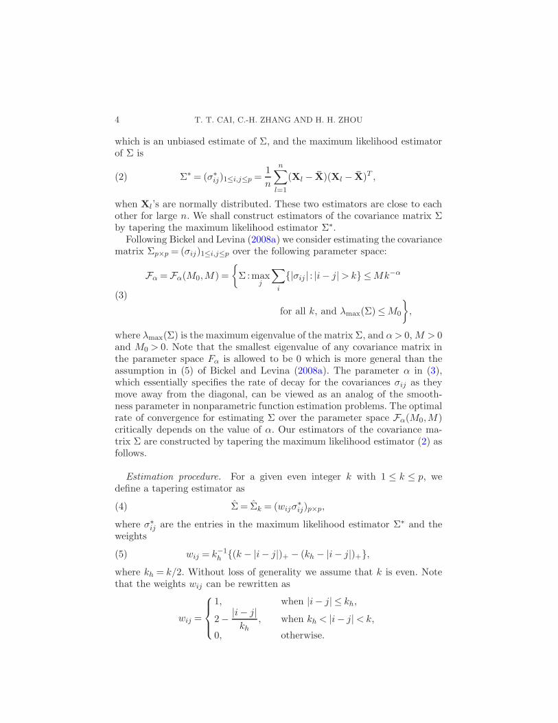
where kh = k/2. Without loss of generality we assume that k is even. Notethat the weights wij can be rewritten as
wij =
1, when |i− j| ≤ kh,
2− |i− j|kh
, when kh < |i− j|< k,
0, otherwise.
COVARIANCE MATRIX ESTIMATION 5
Fig. 1. The weights as a function of |i− j|.
See Figure 1 for a plot of the weights wij as a function of |i− j|.The tapering estimators are different from the banding estimators used
in Bickel and Levina (2008a). It is important to note that the taperingestimator given in (4) can be rewritten as a sum of many small block matricesalong the diagonal. This simple but important observation is very useful forour technical arguments. Define the block matrices
M∗(m)l = (σ∗ijI{l≤ i < l+m, l≤ j < l+m})p×p
and set
S∗(m) =
p∑
l=1−m
M∗(m)l
for all integers 1−m≤ l≤ p and m≥ 1.
Lemma 1. The tapering estimator Σk given in (4) can be written as
Σk = k−1h (S∗(k) − S∗(kh)).(6)
It is clear that the performance of the estimator Σk depends on the choiceof the tapering parameter k. The optimal choice of k critically depends on

6 T. T. CAI, C.-H. ZHANG AND H. H. ZHOU
the norm under which the estimation error is measured. We will study in thenext two sections the rate of convergence of the tapering estimator underboth the operator norm and Frobenius norm. Together with the minimaxlower bounds derived in Sections 3 and 4, the results show that a tapering es-timator with the optimal choice of k attains the optimal rate of convergenceunder these two norms.
3. Rate optimality under the operator norm. In this section we will es-tablish the optimal rate of convergence under the operator norm. For 1≤ q ≤∞, the matrix ℓq-norm of a matrix A is defined by ‖A‖q =max‖x‖q=1‖Ax‖q .The commonly used operator norm ‖ · ‖ coincides with the matrix ℓ2-norm‖ · ‖2. For a symmetric matrix A, it is known that the operator norm ‖A‖ isequal to the largest magnitude of eigenvalues of A. Hence it is also called thespectral norm. We will establish Theorem 1 by deriving a minimax upperbound using the tapering estimator and a matching minimax lower boundby a careful construction of a collection of multivariate normal distribu-tions and the application of Assouad’s lemma and Le Cam’s method. Weshall focus on the case p ≥ n1/(2α+1) in Sections 3.1 and 3.2. The case ofp < n1/(2α+1), which will be discussed in Section 3.3, is similar and slightlyeasier.
3.1. Minimax upper bound under the operator norm. We derive in thissection the risk upper bound for the tapering estimators defined in (6) un-der the operator norm. Throughout the paper we denote by C a genericpositive constant which may vary from place to place but always dependsonly on indices α, M0 and M of the matrix family. We shall assume thatthe distribution of the Xi’s is sub-Gaussian in the sense that there is ρ > 0such that
P{|vT (X1 −EX1)|> t} ≤ e−t2ρ/2 for all t > 0 and ‖v‖2 = 1.(7)
Let Pα =Pα(M0,M,ρ) denote the set of distributions of X1 that satisfy (3)and (7).
Theorem 2. The tapering estimator Σk, defined in (6), of the covari-ance matrix Σp×p with p≥ n1/(2α+1) satisfies
supPα
E‖Σk −Σ‖2 ≤Ck+ log p
n+Ck−2α(8)
for k = o(n), log p= o(n) and some constant C > 0. In particular, the esti-
mator Σ = Σk with k = n1/(2α+1) satisfies
supPα
E‖Σ−Σ‖2 ≤Cn−2α/(2α+1) +Clog p
n.(9)

COVARIANCE MATRIX ESTIMATION 7
From (8) it is clear that the optimal choice of k is of order n1/(2α+1). Theupper bound given in (9) is thus rate optimal among the class of the taperingestimators defined in (6). The minimax lower bound derived in Section 3.2
shows that the estimator Σk with k = n1/(2α+1) is in fact rate optimal amongall estimators.
Proof of Theorem 2. Note that Σ∗ is translation invariant and so isΣ. We shall thus assume µ= 0 for the rest of the paper. Write
Σ∗ =1
n
n∑
l=1
(Xl − X)(Xl − X)T =1
n
n∑
l=1
XlXTl − XX
T,
where XXT
is a higher order term (see Remark 1 at the end of this sec-tion). In what follows we shall ignore this negligible term and focus on thedominating term 1
n
∑nl=1XlX
Tl .
Set Σ = 1n
∑nl=1XlX
Tl and write Σ = (σij)1≤i,j≤p. Let
Σ = (σij)1≤i,j≤p = (wij σij)1≤i,j≤p(10)
with wij given in (5). Let Xl = (X l1,X
l2, . . . ,X
lp)
T . We then write σij =1n
∑nl=1X
liX
lj . It is easy to see
Eσij = σij ,(11)
Var(σij) =1
nVar(X l
iXlj)≤
1
nE(X l
iXlj)
2 ≤ 1
n[E(X l
i)4]1/2[E(X l
j)4]1/2 ≤ C
n,(12)
that is, σij is an unbiased estimator of σij with a variance O(1/n).We will first show that the variance part satisfies
E‖Σ−EΣ‖2 ≤Ck+ log p
n(13)
and the bias part satisfies
‖EΣ−Σ‖2 ≤Ck−2α.(14)
It then follows immediately that
E‖Σ−Σ‖2 ≤ 2E‖Σ−EΣ‖2 +2‖EΣ−Σ‖2 ≤ 2C
(
k+ log p
n+ k−2α
)
.
This proves (8) and equation (9) then follows. Since p≥ n1/(2α+1), we maychoose
k = n1/(2α+1)(15)
and the estimator Σ with k given in (15) satisfies
E‖Σ−Σ‖2 ≤ 2C
(
n−2α/(2α+1) +log p
n
)
.

8 T. T. CAI, C.-H. ZHANG AND H. H. ZHOU
Theorem 2 is then proved. �
We first prove the risk upper bound (14) for the bias part. It is well knownthat the operator norm of a symmetric matrix A= (aij)p×p is bounded byits ℓ1 norm, that is,
‖A‖ ≤ ‖A‖1 = maxi=1,...,p
p∑
j=1
|aij |
[see, e.g., page 15 in Golub and Van Loan (1983)]. This result was used inBickel and Levina (2008a, 2008b) to obtain rates of convergence for theirproposed procedures under the operator norm (see discussions in Section
3.3). We bound the operator norm of the bias part EΣ−Σ by its ℓ1 norm.Since Eσij = σij , we have
EΣ−Σ= ((wij − 1)σij)p×p,
where wij ∈ [0,1] and is exactly 1 when |i− j| ≤ k, then
‖EΣ−Σ‖2 ≤[
maxi=1,...,p
∑
j : |i−j|>k
|σij|]2
≤M2k−2α.
Now we establish (13) which is relatively complicated. The key idea inthe proof is to write the whole matrix as an average of matrices whichare sum of a large number of small disjoint block matrices, and for eachsmall block matrix the classical random matrix theory can be applied. Thefollowing lemma shows that the operator norm of the random matrix Σ−EΣ
is controlled by the maximum of operator norms of p number of k×k random
matrices. Let M(m)l = (σijI{l≤ i < l+m, l≤ j < l+m})p×p. Define
N(m)l = max
1≤l≤p−m+1‖M (m)
l −EM(m)l ‖.
Lemma 2. Let Σ be defined as in (6). Then
‖Σ− EΣ‖ ≤ 3N(m)l .
For each small m×m random matrix with m= k, we control its operatornorm as follows.
Lemma 3. There is a constant ρ1 > 0 such that
P{N (m)l >x} ≤ 2p5m exp(−nx2ρ1)(16)
for all 0<x< ρ1 and 1−m≤ l≤ p.
COVARIANCE MATRIX ESTIMATION 9
With Lemmas 2 and 3 we are now ready to show the variance bound (13).By Lemma 2 we have
E‖Σ− EΣ‖2 ≤ 9E(N(m)l )2 = 9E(N
(m)l )2[I(N
(m)l ≤ x) + I(N
(m)l > x)]
≤ 9[x2 + E(N(m)l )2I(N
(m)l >x)].
Note that ‖EΣ‖ ≤ ‖Σ‖, which is bounded by a constant, and ‖Σ‖ ≤ ‖Σ‖F .The Cauchy–Schwarz inequality then implies
E‖Σ− EΣ‖2 ≤C1[x2 + E(‖Σ‖2F +C)I(N
(m)l > x)]
≤C1[x2 +
√
E(‖Σ‖F +C)4√
P(N(m)l > x)].
Set x= 4√
log p+mnρ1
. Then x is bounded by ρ1 as n→∞. From Lemma 3 we
obtain
E‖Σ−EΣ‖2 ≤ C
[
log p+m
n+ p2 · (p5m · p−8e−8m)1/2
]
(17)
≤ C1
(
log p+m
n
)
.
Remark 1. In the proof of Theorem 2, the term XXTwas ignored. It is
not difficult to see that this term has negligible contribution after tapering.
Let H = XXTand H = (hij)p×p. Define
H(m)l = (hijI{l ≤ i < l+m, l≤ j < l+m})p×p.
Similarly to Lemma 3, it can be shown that
P
{
max1≤l≤p−m+1
‖H(m)l −EH
(m)l ‖> t
}
≤ 2p5m exp(−ntρ2)(18)
for all 0< t< ρ2 and 1−m≤ l≤ p. Note that EH = 1nΣ, then
E‖H‖2 ≤ 2E‖H − EH‖2 +2‖EH‖2 ≤ 2E‖H − EH‖2 +2M20 /n
2.
Let t= 16 log p+mnρ2
. From (18) we have
E‖H −EH‖2 ≤ t2 +E‖H − EH‖2I(
max1≤l≤p−m+1
‖H(m)l −EH
(m)l ‖> t
)
= t2 + o(t2)≤C
(
log p+m
n
)2
by similar arguments as for (17). Therefore H has a negligible contributionto the risk.
10 T. T. CAI, C.-H. ZHANG AND H. H. ZHOU
3.2. Lower bound under the operator norm. Theorem 2 in Section 3.1shows that the optimal tapering estimator attains the rate of convergencen−2α/(2α+1)+ log p
n . In this section we shall show that this rate of convergenceis indeed optimal among all estimators by showing that the upper bound inequation (9) cannot be improved. More specifically we shall show that thefollowing minimax lower bound holds.
Theorem 3. Suppose p≤ exp(γn) for some constant γ > 0. The mini-max risk for estimating the covariance matrix Σ over Pα under the operatornorm satisfies
infΣ
supPα
E‖Σ−Σ‖2 ≥ cn−2α/(2α+1) + clog p
n.
The basic strategy underlying the proof of Theorem 3 is to carefully con-struct a finite collection of multivariate normal distributions and calculatethe total variation affinity between pairs of probability measures in the col-lection.
We shall now define a parameter space that is appropriate for the minimaxlower bound argument. For given positive integers k and m with 2k ≤ p and1≤m≤ k, define the p× p matrix B(m,k) = (bij)p×p with
bij = I{i=m and m+1≤ j ≤ 2k, or j =m and m+1≤ i≤ 2k}.Set k = n1/(2α+1) and a= k−(α+1). We then define the collection of 2k co-variance matrices as
F11 =
{
Σ(θ) :Σ(θ) = Ip + τa
k∑
m=1
θmB(m,k), θ = (θm) ∈ {0,1}k}
,(19)
where Ip is the p× p identity matrix and 0< τ < 2−α−1M . Without loss ofgenerality we assume thatM0 > 1 and ρ > 1. Otherwise we replace Ip in (19)by εIp for 0< ε<min{M0, ρ}. For 0< τ < 2−α−1M it is easy to check thatF11 ⊂Fα(M0,M) as n→∞. In addition to F11 we also define a collectionof diagonal matrices
F12 =
{
Σm :Σm = Ip +
(
√
τ
nlog p1I{i= j =m}
)
p×p
,0≤m≤ p1
}
,(20)
where p1 =min{p, en/2} and 0< τ <min{(M0 − 1)2, (ρ− 1)2,1}. Let F1 =F11 ∪F12. It is clear that F1 ⊂Fα(M0,M).
We shall show below separately that the minimax risks over multivariatenormal distributions with covariance matrix in (19) and (20) satisfy
infΣ
supF11
E‖Σ−Σ‖2 ≥ cn−2α/(2α+1)(21)

COVARIANCE MATRIX ESTIMATION 11
and
infΣ
supF12
E‖Σ−Σ‖2 ≥ clog p
n(22)
for some constant c > 0. Equations (21) and (22) together imply
infΣ
supF1
E‖Σ−Σ‖2 ≥ c
2
(
n−2α/(2α+1) +log p
n
)
(23)
for multivariate normal distributions and this proves Theorem 3. We shallestablish the lower bound (21) by using Assouad’s lemma in Section 3.2.1 andthe lower bound (22) by using Le Cam’s method and a two-point argumentin Section 3.2.2.
3.2.1. A lower bound by Assouad’s lemma. The key technical tool toestablish equation (21) is Assouad’s lemma in Assouad (1983). It gives alower bound for the maximum risk over the parameter set Θ = {0,1}k tothe problem of estimating an arbitrary quantity ψ(θ), belonging to a metric
space with metric d. Let H(θ, θ′) =∑k
i=1 |θi − θ′i| be the Hamming distanceon {0,1}k , which counts the number of positions at which θ and θ′ differ.For two probability measures P and Q with density p and q with respectto any common dominating measure µ, write the total variation affinity‖P ∧Q‖=
∫
p∧ q dµ. Assouad’s lemma provides a minimax lower bound forestimating ψ(θ).
Lemma 4 (Assouad). Let Θ = {0,1}k and let T be an estimator basedon an observation from a distribution in the collection {Pθ, θ ∈Θ}. Then forall s > 0
maxθ∈Θ
2sEθds(T,ψ(θ))≥ min
H(θ,θ′)≥1
ds(ψ(θ), ψ(θ′))H(θ, θ′)
· k2· minH(θ,θ′)=1
‖Pθ ∧ Pθ′‖.
Assouad’s lemma is connected to multiple comparisons. In total thereare k comparisons. The lower bound has three factors. The first factor isbasically the minimum cost of making a mistake per comparison, and thelast factor is the lower bound for the total probability of making type Iand type II errors for each comparison, and k/2 is the expected number ofmistakes one makes when Pθ and Pθ′ are not distinguishable from each otherwhen H(θ, θ′) = 1.
We now prove the lower bound (21). Let X1, . . . ,Xni.i.d.∼ N(0,Σ(θ)) with
Σ(θ) ∈F11. Denote the joint distribution by Pθ. Applying Assouad’s lemmato the parameter space F11, we have
infΣ
maxθ∈{0,1}k
22Eθ‖Σ−Σ(θ)‖2

12 T. T. CAI, C.-H. ZHANG AND H. H. ZHOU
(24)
≥ minH(θ,θ′)≥1
‖Σ(θ)−Σ(θ′)‖2H(θ, θ′)
k
2min
H(θ,θ′)=1‖Pθ ∧Pθ′‖.
We shall state the bounds for the the first and third factors on the right-hand side of (24) in two lemmas. The proofs of these lemmas are given inSection 7.
Lemma 5. Let Σ(θ) be defined as in (19). Then for some constant c > 0
minH(θ,θ′)≥1
‖Σ(θ)−Σ(θ′)‖2H(θ, θ′)
≥ cka2.
Lemma 6. Let X1, . . . ,Xni .i .d .∼ N(0,Σ(θ)) with Σ(θ) ∈ F11. Denote the
joint distribution by Pθ. Then for some constant c > 0
minH(θ,θ′)=1
‖Pθ ∧Pθ′‖ ≥ c.
It then follows from Lemmas 5 and 6 together, with the fact k = n1/(2α+1),
maxΣ(θ)∈F11
22Eθ‖Σ−Σ(θ)‖2 ≥ c2
2k2a2 ≥ c1n
−2α/(2α+1)
for some c1 > 0.
3.2.2. A lower bound using Le Cam’s method. We now apply Le Cam’smethod to derive the lower bound (22) for the minimax risk. Let X be anobservation from a distribution in the collection {Pθ, θ ∈ Θ} where Θ ={θ0, θ1, . . . , θp1}. Le Cam’s method, which is based on a two-point test-ing argument, gives a lower bound for the maximum estimation risk overthe parameter set Θ. More specifically, let L be the loss function. Definer(θ0, θm) = inft[L(t, θ0) + L(t, θm)] and rmin = inf1≤m≤p1 r(θ0, θm), and de-note P= 1
p1
∑p1m=1 Pθm .
Lemma 7. Let T be an estimator of θ based on an observation from adistribution in the collection {Pθ, θ ∈Θ= {θ0, θ1, . . . , θp1}}, then
supθ
EL(T, θ)≥ 1
2rmin‖Pθ0 ∧ P‖.
We refer to Yu (1997) for more detailed discussions on Le Cam’s method.To apply Le Cam’s method, we need to first construct a parameter set.
For 1 ≤m ≤ p1, let Σm be a diagonal covariance matrix with σmm = 1 +√
τ log p1n , σii = 1 for i 6= m, and let Σ0 be the identity matrix. Let Xl =
COVARIANCE MATRIX ESTIMATION 13
(X l1,X
l2, . . . ,X
lp)
T ∼ N(0,Σm), and denote the joint density of X1, . . . ,Xn
by fm, 0≤m≤ p1 with p1 =max{p, en/2}, which can be written as follows:
fm =∏
1≤i≤n,1≤j≤p,j 6=m
φ1(xij) ·
∏
1≤i≤n
φσmm(xim),
where φσ , σ = 1 or σmm, is the density of N(0, σ2). Denote by f0 the jointdensity of X1, . . . ,Xn when Xl ∼N(0,Σ0).
Let θm = Σm for 0 ≤ m ≤ p1 and the loss function L be the squaredoperator norm. It is easy to see r(θ0, θm) = 1
2τlog p1n for all 1≤m≤ p1. Then
the lower bound (22) follows immediately from Lemma 7 if there is a constantc > 0 such that
‖Pθ0 ∧ P‖ ≥ c.(25)
Note that for any two densities q0 and q1,∫
q0∧q1 dµ= 1− 12
∫
|q0−q1|dµ,and Jensen’s inequality implies[∫
|q0 − q1|dµ]2
=
(∫∣
∣
∣
∣
q0 − q1q1
∣
∣
∣
∣
q1 dµ
)2
≤∫
(q0 − q1)2
q1dµ=
∫
q20q1dµ− 1.
Hence∫
q0∧ q1 dµ≥ 1− 12(∫ q20
q1dµ−1)1/2. To establish equation (25), it thus
suffices to show that∫
( 1p1
∑p1m=1 fm)2/f0 dµ− 1→ 0, that is,
1
p21
p1∑
m=1
∫
f2mf0
dµ+1
p21
∑
m6=j
∫
fmfjf0
dµ− 1→ 0.(26)
We now calculate∫ fmfj
f0dµ. For m 6= j it is easy to see∫
fmfjf0
dµ− 1 = 0.
When m= j, we have∫
f2mf0
dµ=(√2πσmm)−2n
(√2π)−n
∏
1≤i≤n
∫
exp
[
(xim)2(
− 1
σmm+
1
2
)]
dxim
= [1− (1− σmm)2]−n/2 =
(
1− τlog p1n
)−n/2
.
Thus∫
(
1
p1
p1∑
m=1
fm
)2/
f0 dµ− 1
=1
p21
p1∑
m=1
(∫
f2mf0
dµ− 1
)
14 T. T. CAI, C.-H. ZHANG AND H. H. ZHOU
(27)
≤ 1
p1
(
1− τlog p1n
)−n/2
− 1
p1
= exp
[
− log p1 −n
2log
(
1− τlog p1n
)]
− 1
p1→ 0
for 0< τ < 1, where the last step follows from the inequality log(1−x)≥−2xfor 0 < x < 1/2. Equation (27), together with Lemma 7, now immediatelyimplies the lower bound given in (22).
Remark 2. In covariance matrix estimation literature, it is commonlyassumed that log p
n → 0. See, for example, Bickel and Levina (2008a). Thelower bound given in this section implies that this assumption is necessaryfor estimating the covariance matrix consistently under the operator norm.
3.3. Discussion. Theorems 2 and 3 together show that the minimax riskfor estimating the covariance matrices over the distribution space Pα satis-fies, for p≥ n1/(2α+1),
infΣ
supPα
E‖Σ−Σ‖2 ≍ n−2α/(2α+1) +log p
n.(28)
The results also show that the tapering estimator Σk with tapering parame-ter k = n1/(2α+1) attains the optimal rate of convergence n−2α/(2α+1)+ log p
n .A few interesting points can be made on the optimal rate of convergence
n−2α/(2α+1)+ log pn . When the dimension p is relatively small, that is, log p=
o(n1/(2α+1)), p has no effect on the convergence rate and the rate is purelydriven by the “smoothness” parameter α. However, when p is large, that is,log p≫ n1/(2α+1), p plays a significant role in determining the minimax rate.
We should emphasize that the optimal choice of the tapering param-eter k ≍ n1/(2α+1) is different from the optimal choice for estimating therows/columns as vectors under mean squared error loss. Straightforwardcalculation shows that in the latter case the best cutoff is k ≍ n1/(2(α+1))
so that the tradeoff between the squared bias and the variance is optimal.With k ≍ n1/(2α+1), the tapering estimator has smaller squared bias thanthe variance as a vector estimator of each row/column.
It is also interesting to compare our results with those given in Bickel andLevina (2008a). A banding estimator with bandwidth k = ( log pn )1/(2(α+1))
was proposed and the rate of convergence ( log pn )α/(α+1) was proved. It iseasy to see that the banding estimator given in Bickel and Levina (2008a)
is not rate optimal. Take, for example, α= 1/2 and p = e√n. Their rate is
n−1/6, while the optimal rate in Theorem 1 is n−1/2.

COVARIANCE MATRIX ESTIMATION 15
It is instructive to take a closer look at the motivation behind the con-struction of the banding estimator in Bickel and Levina (2008a). Let thebanding estimator be
ΣB = (σ∗ijI{|i− j| ≤ k})(29)
and denote ΣB − EΣB by V , and let V = (vij). An important step in theproof of Theorem 1 in Bickel and Levina (2008a) is to control the operatornorm by the ℓ1 norm as follows:
E‖ΣB − EΣB‖2 ≤ E‖ΣB −EΣB‖21 = E
(
maxj=1,...,p
∑
i
|vij |)2
≤ C
(
k√n
√
log p
)2
=Ck2 log p
n.
Note that E[|vij |I{|i− j| ≤ k}] ≍ 1/√n, then E
∑
i |vij | ≍ k/√n. It is then
expected that E(maxj=1,...,p∑
i |vij |)2 ≤ C( k√n
√log p)2 [see Bickel and Lev-
ina (2008a) for details] and so
E‖Σ−Σ‖21 ≤Ck2 log p
n+Ck−2α.
An optimal tradeoff of k is then ( log pn )1/(2(α+1)) which implies a rate of
( log pn )−α/(α+1) in Theorem 1 in Bickel and Levina (2008a). This rate is slower
than the optimal rate n−2α/(2α+1) + log pn in Theorem 1.
We have considered the parameter space Fα defined in (3). Other similarparameter spaces can also be considered. For example, in time series analysisit is often assumed the covariance |σij | decays at the rate |i− j|−(α+1) forsome α > 0. Consider the collection of positive-definite symmetric matricessatisfying the following conditions:
Gα = Gα(M0,M1)(30)
= {Σ: |σij| ≤M1|i− j|−(α+1) for i 6= j and λmax(Σ)≤M0},
where λmax(Σ) is the maximum eigenvalues of the matrix Σ. Note thatGα(M0, M1) is a subset of Fα(M0,M) as long as M1 ≤ αM . Using virtuallyidentical arguments one can show that
infΣ
supP ′α
E‖Σ−Σ‖2 ≍ n−2α/(2α+1) +log p
n.
Let P ′α = P ′
α(M0,M,ρ) denote the set of distributions of X1 that satisfies(7) and (30).
16 T. T. CAI, C.-H. ZHANG AND H. H. ZHOU
Remark 3. Both the tapering estimator proposed in this paper andbanding estimator given in Bickel and Levina (2008a) are not necessarilypositive-semidefinite. A practical proposal to avoid this would be to projectthe estimator Σ to the space of positive-semidefinite matrices under theoperator norm. More specifically, one may first diagonalize Σ and then re-place negative eigenvalues by 0. The resulting estimator is then positive-semidefinite.
3.3.1. The case of p < n1/(2α+1). We have focused on the case p≥ n1/(2α+1)
in Sections 3.1 and 3.2. The case of p < n1/(2α+1) can be handled in a similarway. The main difference is that in this case we no longer have a taperingestimator Σk with k = n1/(2α+1) because k > p. Instead the maximum like-lihood estimator Σ∗ can be used directly. It is easy to show in this case
supPα
E‖Σ∗ −Σ‖2 ≤Cp
n.(31)
The lower bound can also be obtained by the application of Assouad’s lemmaand by using a parameter space that is similar to F11. To be more specific,for an integer 1≤m≤ p/2, define the p× p matrix Bm = (bij)p×p with
bij = I{i=m and m+1≤ j ≤ p, or j =m and m+1≤ i≤ p}.
Define the collection of 2p/2 covariance matrices as
F∗ =
{
Σ(θ) :Σ(θ) = Ip + τ1√np
p/2∑
m=1
θmB(m,k), θ = (θm) ∈ {0,1}p/2}
.(32)
Since p < n1/(2α+1), then 1√np < 2α+1/2p−(α+1). Again it is easy to check
F∗ ⊂ Fα(M0,M) when 0 < τ < 2−α−1M . The following lower bound thenfollows from the same argument as in Section 3.2.1:
infΣ
supF∗
E‖Σ−Σ‖2 ≥ cp
(
1√np
)2
· p2· c1 ≥ c2
p
n.(33)
Equations (31) and (33) together yield the minimax rate of convergence forthe case p≤ n1/(2α+1),
infΣ
supPα
E‖Σ−Σ‖2 ≍ p
n.(34)
This, together with equation (28), gives the optimal rate of convergence:
infΣ
supPα
E‖Σ−Σ‖2 ≍min
{
n−2α/(2α+1) +log p
n,p
n
}
.(35)
COVARIANCE MATRIX ESTIMATION 17
4. Rate optimality under the Frobenius norm. In addition to the opera-tor norm, the Frobenius norm is another commonly used matrix norm. TheFrobenius norm is used in defining the numerical rank of a matrix whichis useful in many applications, such as the principle component analysis.See, for example, Rudelson and Vershynin (2007). The Frobenius norm hasalso been used in the literature for measuring the accuracy of a covariancematrix estimator. See, for example, Lam and Fan (2007) and Ravikumaret al. (2008). In this section we consider the optimal rate of convergencefor covariance matrix estimation under the Frobenius norm. The Frobeniusnorm of a matrix A= (aij) is defined as the ℓ2 vector norm of all entries inthe matrix
‖A‖F =
√
∑
i,j
a2ij .
This is equivalent to treating the matrix A as a vector of length p2. It iseasy to see that the operator norm is bounded by the Frobenius norm, thatis, ‖A‖ ≤ ‖A‖F .
The following theorem gives the minimax rate of convergence for estimat-ing the covariance matrix Σ under the Frobenius norm based on the sample{X1, . . . ,Xn}.
Theorem 4. The minimax risk under the Frobenius norm satisfies
infΣ
supPα
E1
p‖Σ−Σ‖2F ≍ inf
ΣsupP ′α
E1
p‖Σ−Σ‖2F
(36)
≍min
{
n−(2α+1)/(2(α+1)),p
n
}
.
We shall establish below separately the minimax upper bound and mini-max lower bound.
4.1. Upper bound under the Frobenius norm. We will only prove the up-per bound for the distribution set P ′
α given in (30). The proof for the pa-rameter space Pα is slightly more involved by thresholding procedures as inWavelet estimation. The minimax upper bound is derived by again consider-ing the tapering estimator (4). Under the Frobenius norm the risk functionis separable. The risk of the tapering estimator can be bounded separatelyunder the squared ℓ2 loss for each row/column. This method has been com-monly used in nonparametric function estimation using orthogonal basisexpansions. Since
Eσij = σij and Var(σij)≤C
n

18 T. T. CAI, C.-H. ZHANG AND H. H. ZHOU
for the tapering estimator (4), we have
E(wijσij − σij)2 ≤ (1−wij)
2σ2ij +w2ij
C
n.
It can be seen easily that
1
pE‖Σ−Σ‖2F ≤ 1
p
∑
{(i,j) : kh<|i−j|}σ2ij +
1
p
∑
{(i,j) : |i−j|≤k}
[
(1−wij)2σ2ij +w2
ij
C
n
]
≡R1 +R2.
The assumption λmax(Σ)≤M0 implies that σii ≤M0 for all i. Since |σij| isalso uniformly bounded for all i 6= j from assumption (30), we immediatelyhave R2 ≤C k
n .It is easy to show that
1
p
∑
{(i,j) : k<|i−j|}σ2ij ≤Ck−2α−1,(37)
where |σij | ≤C1|i− j|−(α+1) for all i 6= j. Thus
E1
p‖Σ−Σ‖2F ≤Ck−2α−1 +C
k
n≤C2n
−(2α+1)/(2(α+1))(38)
by choosing
k = n1/(2(α+1))(39)
if n1/(2(α+1)) ≤ p, which is different from the choice of k for the operatornorm in (15). If n1/(2(α+1)) > p, we will choose k = p, then the bias part is 0and consequently
E1
p‖Σ−Σ‖2F ≤C
p
n.
Remark 4. For the parameter space P ′α, under the Frobenius norm the
optimal tapering parameter k is of the order n1/(2(α+1)). The rate of con-vergence of the tapering estimator with k ≍ n1/(2(α+1)) under the operatornorm is
log p
n+ n−α/(α+1),
which is slower than n−2α/(2α+1) + log pn in (1). Similarly, the optimal pro-
cedure under the operator norm is not rate optimal under the Frobeniusnorm. Therefore, the optimal choice of the tapering parameter k criticallydepends on the norm under which the estimation accuracy is measured.
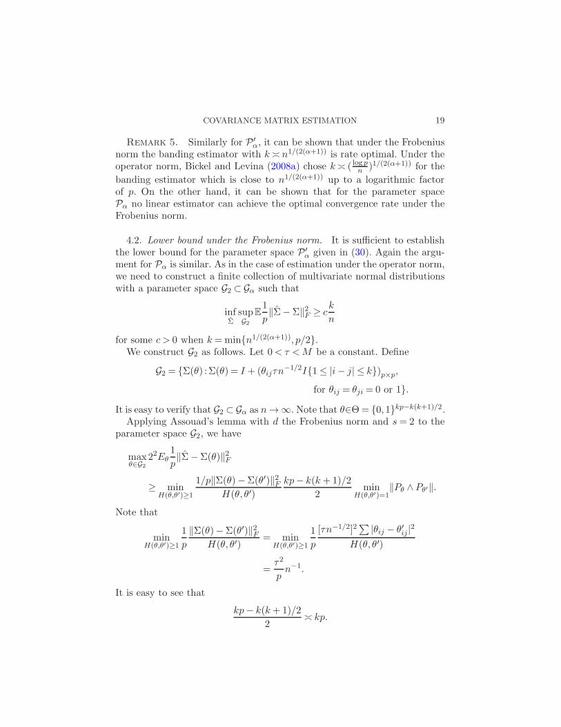
COVARIANCE MATRIX ESTIMATION 19
Remark 5. Similarly for P ′α, it can be shown that under the Frobenius
norm the banding estimator with k ≍ n1/(2(α+1)) is rate optimal. Under theoperator norm, Bickel and Levina (2008a) chose k ≍ ( log pn )1/(2(α+1)) for the
banding estimator which is close to n1/(2(α+1)) up to a logarithmic factorof p. On the other hand, it can be shown that for the parameter spacePα no linear estimator can achieve the optimal convergence rate under theFrobenius norm.
4.2. Lower bound under the Frobenius norm. It is sufficient to establishthe lower bound for the parameter space P ′
α given in (30). Again the argu-ment for Pα is similar. As in the case of estimation under the operator norm,we need to construct a finite collection of multivariate normal distributionswith a parameter space G2 ⊂ Gα such that
infΣ
supG2
E1
p‖Σ−Σ‖2F ≥ c
k
n
for some c > 0 when k =min{n1/(2(α+1)), p/2}.We construct G2 as follows. Let 0< τ <M be a constant. Define
G2 = {Σ(θ) :Σ(θ) = I + (θijτn−1/2I{1≤ |i− j| ≤ k})p×p,
for θij = θji = 0 or 1}.
It is easy to verify that G2 ⊂Gα as n→∞. Note that θ∈Θ= {0,1}kp−k(k+1)/2.Applying Assouad’s lemma with d the Frobenius norm and s= 2 to the
parameter space G2, we have
maxθ∈G2
22Eθ1
p‖Σ−Σ(θ)‖2F
≥ minH(θ,θ′)≥1
1/p‖Σ(θ)−Σ(θ′)‖2FH(θ, θ′)
kp− k(k +1)/2
2min
H(θ,θ′)=1‖Pθ ∧Pθ′‖.
Note that
minH(θ,θ′)≥1
1
p
‖Σ(θ)−Σ(θ′)‖2FH(θ, θ′)
= minH(θ,θ′)≥1
1
p
[τn−1/2]2∑ |θij − θ′ij|2
H(θ, θ′)
=τ2
pn−1.
It is easy to see that
kp− k(k+ 1)/2
2≍ kp.
20 T. T. CAI, C.-H. ZHANG AND H. H. ZHOU
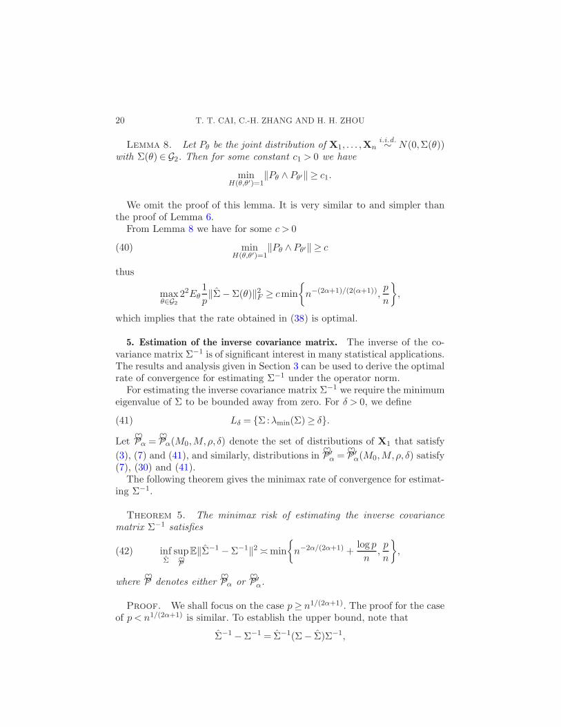
Lemma 8. Let Pθ be the joint distribution of X1, . . . ,Xni .i .d .∼ N(0,Σ(θ))
with Σ(θ)∈ G2. Then for some constant c1 > 0 we have
minH(θ,θ′)=1
‖Pθ ∧Pθ′‖ ≥ c1.
We omit the proof of this lemma. It is very similar to and simpler thanthe proof of Lemma 6.
From Lemma 8 we have for some c > 0
minH(θ,θ′)=1
‖Pθ ∧Pθ′‖ ≥ c(40)
thus
maxθ∈G2
22Eθ1
p‖Σ−Σ(θ)‖2F ≥ cmin
{
n−(2α+1)/(2(α+1)),p
n
}
,
which implies that the rate obtained in (38) is optimal.
5. Estimation of the inverse covariance matrix. The inverse of the co-variance matrix Σ−1 is of significant interest in many statistical applications.The results and analysis given in Section 3 can be used to derive the optimalrate of convergence for estimating Σ−1 under the operator norm.
For estimating the inverse covariance matrix Σ−1 we require the minimumeigenvalue of Σ to be bounded away from zero. For δ > 0, we define
Lδ = {Σ:λmin(Σ)≥ δ}.(41)
Let ♥Pα = ♥Pα(M0,M,ρ, δ) denote the set of distributions of X1 that satisfy
(3), (7) and (41), and similarly, distributions in ♥P ′α = ♥P ′
α(M0,M,ρ, δ) satisfy(7), (30) and (41).
The following theorem gives the minimax rate of convergence for estimat-ing Σ−1.
Theorem 5. The minimax risk of estimating the inverse covariancematrix Σ−1 satisfies
infΣ
sup♥P
E‖Σ−1 −Σ−1‖2 ≍min
{
n−2α/(2α+1) +log p
n,p
n
}
,(42)
where ♥P denotes either ♥Pα or ♥P ′α.
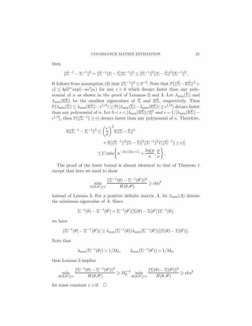
Proof. We shall focus on the case p≥ n1/(2α+1). The proof for the caseof p < n1/(2α+1) is similar. To establish the upper bound, note that
Σ−1 −Σ−1 = Σ−1(Σ− Σ)Σ−1,
COVARIANCE MATRIX ESTIMATION 21
then
‖Σ−1 −Σ−1‖2 = ‖Σ−1(Σ− Σ)Σ−1‖2 ≤ ‖Σ−1‖2‖Σ− Σ‖2‖Σ−1‖2.
It follows from assumption (3) that ‖Σ−1‖2 ≤ δ−2. Note that P{‖Σ−EΣ‖2 >ǫ} ≤ 4p5m exp(−nǫ2ρ1) for any ǫ > 0 which decays faster than any poly-
nomial of n as shown in the proof of Lemmas 2 and 3. Let λmin(Σ) and
λmin(EΣ) be the smallest eigenvalues of Σ and EΣ, respectively. Then
P(λmin(Σ)≤ λmin(EΣ)−ǫ1/2)≥ P(|λmin(Σ)−λmin(EΣ)| ≥ ǫ1/2) decays faster
than any polynomial of n. Let 0< ǫ < [λmin(EΣ)/2]2 and c= 1/[λmin(EΣ)−
ǫ1/2], then P(‖Σ−1‖ ≥ c) decays faster than any polynomial of n. Therefore,
E‖Σ−1 −Σ−1‖2 ≤(
c
δ
)2
E‖Σ− Σ‖2
+E[‖Σ−1‖2‖Σ− Σ‖2‖Σ−1‖2I(‖Σ−1‖ ≥ c)]
≤Cmin
{
n−2α/(2α+1) +log p
n,p
n
}
.
The proof of the lower bound is almost identical to that of Theorem 1except that here we need to show
minH(θ,θ′)≥1
‖Σ−1(θ)−Σ−1(θ′)‖2H(θ, θ′)
≥ cka2
instead of Lemma 5. For a positive definite matrix A, let λmin(A) denotethe minimum eigenvalue of A. Since
Σ−1(θ)−Σ−1(θ′) = Σ−1(θ′)(Σ(θ)−Σ(θ′))Σ−1(θ),
we have
‖Σ−1(θ)−Σ−1(θ′)‖ ≥ λmin(Σ−1(θ))λmin(Σ
−1(θ′))‖Σ(θ)−Σ(θ′)‖.
Note that
λmin(Σ−1(θ))> 1/M0, λmin(Σ
−1(θ′))> 1/M0,
then Lemma 5 implies
minH(θ,θ′)≥1
‖Σ−1(θ)−Σ−1(θ′)‖2H(θ, θ′)
≥M−40 min
H(θ,θ′)≥1
‖Σ(θ)−Σ(θ′)‖2H(θ, θ′)
≥ cka2
for some constant c > 0. �

22 T. T. CAI, C.-H. ZHANG AND H. H. ZHOU
6. Simulation study. We now turn to the numerical performance of theproposed tapering estimator and compare it with that of the banding estima-tor of Bickel and Levina (2008a). In the numerical study, we shall considerestimating a covariance matrix in the parameter space Fα defined in (3).Specifically, we consider the covariance matrix Σ= (σij)1≤i,j≤p of the form
σij =
{
1, 1≤ i= j ≤ p,ρ|i− j|−(α+1), 1≤ i 6= j ≤ p.
(43)
Note that this is a Toeplitz matrix. But we do not assume that the structureis known and do not use the information in any estimation procedure.
The banding estimator in (29) depends on the choice of k. An optimaltradeoff of k is k ≍ (n/ log p)1/(2α+2) as discussed in Section 3.3. See Bickeland Levina (2008a). The tapering estimator (6) also depends on k for whichthe optimal tradeoff is k ≍ n1/(2α+1). In our simulation study, we choosek = ⌊(n/ log p)1/(2α+2)⌋ for the banding estimator and k = ⌊n1/(2α+1)⌋ forthe tapering estimator.
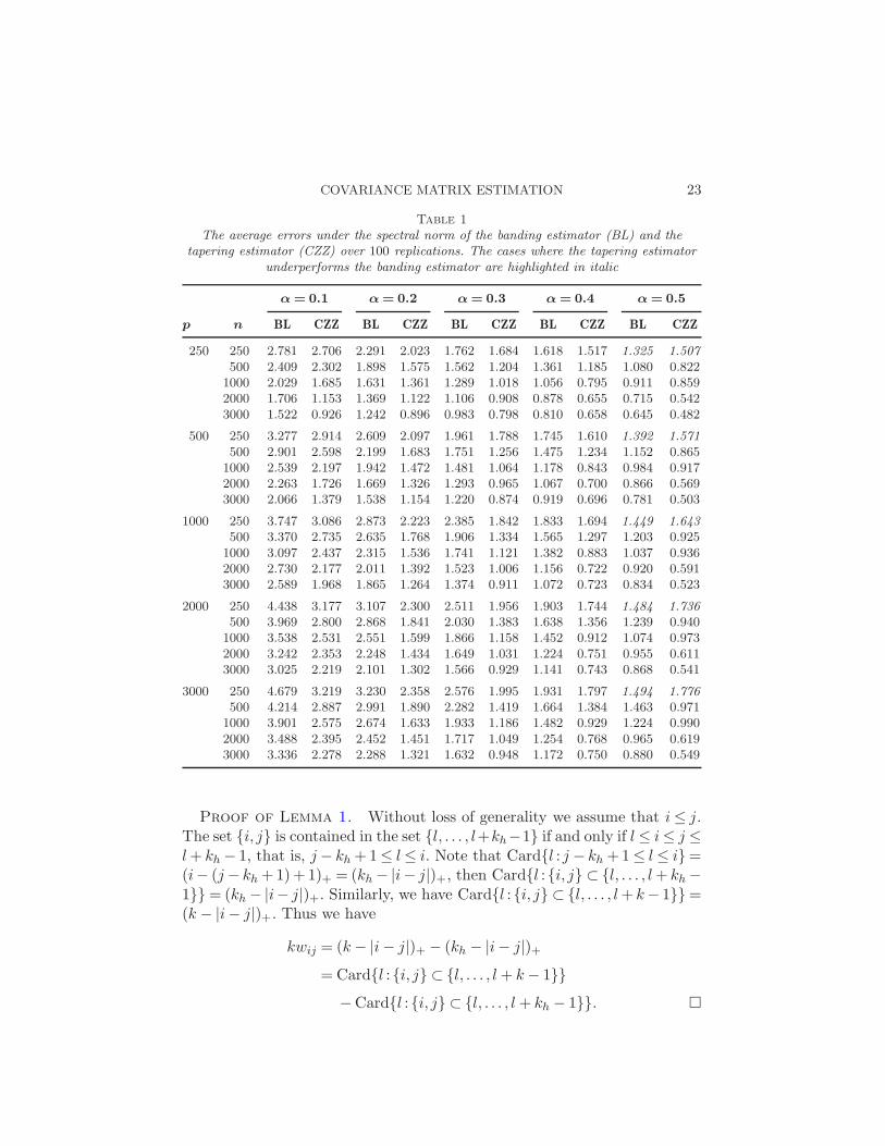
A range of parameter values for α, n and p are considered. Specifically, αranges from 0.1 to 0.5, the sample size n ranges from 250 to 3000 and thedimension p goes from 250 to 3000. We choose the value of ρ to be ρ= 0.6so that all matrices are nonnegative definite and their smallest eigenvaluesare close to 0. Table 1 reports the average errors under the spectral normover 100 replications for the two procedures. The cases where the taperingestimator underperforms the banding estimator are highlighted in boldface.Figure 2 plots the ratios of the average errors of the banding estimator to thecorresponding average errors of the tapering estimator for α = 0.1,0.2,0.3and 0.5. The case of α= 0.4 is similar to the case of α= 0.3.
It can be seen from Table 1 and Figure 2 that the tapering estimatoroutperforms the banding estimator in 121 out of 125 cases. For the givendimension p, the ratio of the average error of the banding estimator to thecorresponding average error of the tapering estimator tends to increase asthe sample size n increases. The tapering estimator fails to outperform thebanding estimator only when α= 0.5 and n= 250 in which case the valuesof k are small for both estimators.
Remark 6. We have also carried out additional simulations for largervalues of α with the same sample sizes and dimensions. The performance ofthe tapering and abnding estimators are similar. This is mainly dur to thefact that the values of k for both estimators are very small for large α whenn and p are only moderately large.
7. Proofs of auxiliary lemmas. In this section we give proofs of auxiliarylemmas stated and used in Sections 3–5.
COVARIANCE MATRIX ESTIMATION 23
Table 1
The average errors under the spectral norm of the banding estimator (BL) and thetapering estimator (CZZ) over 100 replications. The cases where the tapering estimator
underperforms the banding estimator are highlighted in italic
α= 0.1 α= 0.2 α= 0.3 α= 0.4 α= 0.5
p n BL CZZ BL CZZ BL CZZ BL CZZ BL CZZ
250 250 2.781 2.706 2.291 2.023 1.762 1.684 1.618 1.517 1.325 1.507500 2.409 2.302 1.898 1.575 1.562 1.204 1.361 1.185 1.080 0.822
1000 2.029 1.685 1.631 1.361 1.289 1.018 1.056 0.795 0.911 0.8592000 1.706 1.153 1.369 1.122 1.106 0.908 0.878 0.655 0.715 0.5423000 1.522 0.926 1.242 0.896 0.983 0.798 0.810 0.658 0.645 0.482
500 250 3.277 2.914 2.609 2.097 1.961 1.788 1.745 1.610 1.392 1.571500 2.901 2.598 2.199 1.683 1.751 1.256 1.475 1.234 1.152 0.865
1000 2.539 2.197 1.942 1.472 1.481 1.064 1.178 0.843 0.984 0.9172000 2.263 1.726 1.669 1.326 1.293 0.965 1.067 0.700 0.866 0.5693000 2.066 1.379 1.538 1.154 1.220 0.874 0.919 0.696 0.781 0.503
1000 250 3.747 3.086 2.873 2.223 2.385 1.842 1.833 1.694 1.449 1.643500 3.370 2.735 2.635 1.768 1.906 1.334 1.565 1.297 1.203 0.925
1000 3.097 2.437 2.315 1.536 1.741 1.121 1.382 0.883 1.037 0.9362000 2.730 2.177 2.011 1.392 1.523 1.006 1.156 0.722 0.920 0.5913000 2.589 1.968 1.865 1.264 1.374 0.911 1.072 0.723 0.834 0.523
2000 250 4.438 3.177 3.107 2.300 2.511 1.956 1.903 1.744 1.484 1.736500 3.969 2.800 2.868 1.841 2.030 1.383 1.638 1.356 1.239 0.940
1000 3.538 2.531 2.551 1.599 1.866 1.158 1.452 0.912 1.074 0.9732000 3.242 2.353 2.248 1.434 1.649 1.031 1.224 0.751 0.955 0.6113000 3.025 2.219 2.101 1.302 1.566 0.929 1.141 0.743 0.868 0.541
3000 250 4.679 3.219 3.230 2.358 2.576 1.995 1.931 1.797 1.494 1.776500 4.214 2.887 2.991 1.890 2.282 1.419 1.664 1.384 1.463 0.971
1000 3.901 2.575 2.674 1.633 1.933 1.186 1.482 0.929 1.224 0.9902000 3.488 2.395 2.452 1.451 1.717 1.049 1.254 0.768 0.965 0.6193000 3.336 2.278 2.288 1.321 1.632 0.948 1.172 0.750 0.880 0.549
Proof of Lemma 1. Without loss of generality we assume that i≤ j.The set {i, j} is contained in the set {l, . . . , l+kh−1} if and only if l≤ i≤ j ≤l+ kh − 1, that is, j− kh +1≤ l≤ i. Note that Card{l : j − kh +1≤ l≤ i}=(i− (j− kh +1)+1)+ = (kh − |i− j|)+, then Card{l :{i, j} ⊂ {l, . . . , l+ kh−1}}= (kh − |i− j|)+. Similarly, we have Card{l :{i, j} ⊂ {l, . . . , l+ k− 1}}=(k − |i− j|)+. Thus we have
kwij = (k− |i− j|)+ − (kh − |i− j|)+=Card{l :{i, j} ⊂ {l, . . . , l+ k− 1}}
−Card{l :{i, j} ⊂ {l, . . . , l+ kh − 1}}. �

24 T. T. CAI, C.-H. ZHANG AND H. H. ZHOU
Fig. 2. The vertical bars represent the ratios of the average error of the banding estimatorto the corresponding average error of the tapering estimator. The higher the bar the betterthe relative performance of the tapering estimator. For each value of p the bars are orderedfrom left to right by the sample sizes (n= 250 to 3000).

COVARIANCE MATRIX ESTIMATION 25
Proof of Lemma 2. Without loss of generality we assume that p is
divisible by m. Recall that M(m)l = (σijI{l ≤ i < l +m, l ≤ j < l +m})p×p.
Note that M(m)l is empty when l ≤ 1 −m, and has at least one nonzero
entry when l≥ 2−m. Set δ(m)l =M
(m)l −EM
(m)l and S(m) =
∑pl=2−mM
(m)l .
It follows from (6) that
‖S(m) −ES(m)‖ ≤m∑
l=1
∥
∥
∥
∥
∑
−1≤j<p/m
δ(m)jm+l
∥
∥
∥
∥
.(44)
Since δ(m)jm+l are disjoint diagonal blocks over −1≤ j < p/m, we have
‖S(m) − ES(m)‖ ≤m max1≤l≤m
∥
∥
∥
∥
∑
−1≤j<p/m
δ(m)jm+l
∥
∥
∥
∥
(45)≤m max
1−m≤l≤p‖δ(m)
l ‖.
Since δ(kh)l and δ
(k)l are all sub-blocks of certain matrix δ
(k)l with 1 ≤ l ≤
p− k + 1, Lemma 2 now follows immediately from equations (45) and (6).�
Proof of Lemma 3. For any m×m symmetric matrix A, we have
|uTAu| − |vTAv| ≤ |uTAu− vTAv|= |(u− v)TA(u+ v)|≤ ‖u− v‖‖A‖‖u+ v‖.
Let Sm−11/2 be a 1/2 net of the unit sphere Sm−1 in the Euclidean distance
in Rm. We have
‖A‖ ≤ supu∈Sm−1
|uTAu| ≤ supu∈Sm−1
1/2
|uTAu|+ 1
2‖A‖3
2
= supu∈Sm−1
1/2
|uTAu|+ 3
4‖A‖,
which implies ‖A‖ ≤ 4 supu∈Sm−11/2
|uTAu|. Since we are allowed to pack
Card(Sm−11/2 ) balls of radius 1/4 into a 1 + 1/4 ball in Rm, volume com-
parison yields
(1/4)mCard(Sm−11/2 )≤ (5/4)m,
that is, Card(Sm−11/2 )≤ 5m. Thus there exist v1,v2, . . . ,v5m ∈ Sm−1 such that
‖A‖ ≤ 4 supj≤5m
|vTj Avj | for all m×m symmetric A.

26 T. T. CAI, C.-H. ZHANG AND H. H. ZHOU
This one-step approximation argument is similar to the proof of Proposition4.2(ii) in Zhang and Huang (2008).
Let X1, . . . ,Xn be i.i.d. p-vectors with E(X1−µ)(X1−µ)T =Σ. Under thesub-Gaussian assumption in (7) there exists ρ > 0 such that
P{vT (Xi −EXi)(Xi −EXi)Tv> x} ≤ e−xρ/2 for all x> 0 and ‖v‖= 1,
which implies E(tvT (Xi−EXi)(Xi−EXi)Tv)<∞ for all t < ρ/2 and ‖v‖=
1, then there exists ρ1 > 0 such that
P
{∣
∣
∣
∣
∣
1
n
n∑
i=1
vT [(Xi − EXi)(Xi −EXi)
T −Σ]v
∣
∣
∣
∣
∣
> x
}
≤ e−nx2ρ1/2
for all 0 < x < ρ1 and ‖v‖ = 1. [See, e.g., Chapter 2 in Saulis and Stat-ulevicius (1991).] Thus we have
P
{
max1≤l≤p−m+1
‖M (m)l − EM
(m)l ‖> x
}
≤∑
1≤l≤p−m+1
P{‖M (m)l − EM
(m)l ‖> x}
≤ 2p5m supvj ,l
P{|vTj (M
(m)l −EM
(m)l )vj|>x}
≤ 2p5m exp(−nx2ρ1/2). �
Proof of Lemma 5. Set v = (1{kh ≤ i≤ k}) and let
(wi) = [Σ(θ)−Σ(θ′)]v.
Note that there are exactly H(θ, θ′) number of wi such that |wi|= τkha, and‖v‖22 = kh. This implies
‖Σ(θ)−Σ(θ′)‖2 ≥ ‖[Σ(θ)−Σ(θ′)]v‖22‖v‖22
≥ H(θ, θ′) · (τka)2kh
=H(θ, θ′) · τ2kha2. �
Proof of Lemma 6. When H(θ, θ′) = 1, we will show
‖Pθ′ −Pθ‖21 ≤ 2K(Pθ′ |Pθ)
= 2n
[
1
2tr(Σ(θ′)Σ−1(θ))− 1
2log det(Σ(θ′)Σ−1(θ))− p
2
]
≤ n · cka2
for some small c > 0, where K(·|·) is the Kullback–Leibler divergence andthe first inequality follows from the well-known Pinsker’s inequality [see,

COVARIANCE MATRIX ESTIMATION 27
e.g., Csiszar (1967)]. This immediately implies the L1 distance between twomeasures is bounded away from 1, and then the lemma follows. Write
Σ(θ′) =D1 +Σ(θ).
Then
1
2tr(Σ(θ′)Σ−1(θ))− p
2=
1
2tr(D1Σ
−1(θ)).
Let λi be the eigenvalues of D1Σ−1(θ). Since D1Σ
−1(θ) is similar to thesymmetric matrix Σ−1/2(θ)D1Σ
−1/2(θ), and
‖Σ−1/2(θ)D1Σ−1/2(θ)‖ ≤ ‖Σ−1/2(θ)‖‖D1‖‖Σ−1/2(θ)‖
≤ c1‖D1‖ ≤ c1‖D1‖1 ≤ c2ka,
then all eigenvalues λi’s are real and in the interval [−c2ka, c2ka], whereka= k · k−(α+1) = k−α → 0. Note that the Taylor expansion yields
log det(Σ(θ′)Σ−1(θ)) = log det(I +D1Σ−1(θ)) = tr(D1Σ
−1(θ))−R3,
where
R3 ≤ c3
p∑
i=1
λ2i for some c3 > 0.
Write Σ−1/2(θ) = UV 1/2UT , where UUT = I and V is a diagonal matrix. Itfollows from the fact that the Frobenius norm of a matrix remains the sameafter an orthogonal transformation that
p∑
i=1
λ2i = ‖Σ−1/2(θ)D1Σ−1/2(θ)‖2F ≤ ‖V ‖2 · ‖UTD1U‖2F
= ‖Σ−1(θ)‖2 · ‖D1‖2F ≤ c4ka2. �
Acknowledgments. The authors would like to thank James X. Hu forassistance in carrying out the simulation study in Section 6. We also thankthe Associate Editor and three referees for thorough and useful commentswhich have helped to improve the presentation of the paper.
REFERENCES
Assouad, P. (1983). Deux remarques sur l’estimation. C. R. Acad. Sci. Paris Ser. I Math.296 1021–1024. MR0777600
Bickel, P. J. and Levina, E. (2008a). Regularized estimation of large covariance matrices.Ann. Statist. 36 199–227. MR2387969
Bickel, P. J. and Levina, E. (2008b). Covariance regularization by thresholding. Ann.Statist. 36 2577–2604. MR2485008
28 T. T. CAI, C.-H. ZHANG AND H. H. ZHOU
Csiszar, I. (1967). Information-type measures of difference of probability distributions
and indirect observation. Studia Sci. Math. Hungar. 2 229–318. MR0219345
El Karoui, N. (2008). Operator norm consistent estimation of large dimensional sparse
covariance matrices. Ann. Statist. 36 2717–2756. MR2485011
Golub, G. H. and Van Loan, C. F. (1983). Matrix Computations. John Hopkins Univ.
Press, Baltimore. MR0733103
Fan, J., Fan, Y. and Lv, J. (2008). High dimensional covariance matrix estimation using
a factor model. J. Econometrics 147 186–197. MR2472991
Furrer, R. and Bengtsson, T. (2007). Estimation of high-dimensional prior and pos-
terior covariance matrices in Kalman filter variants. J. Multivariate Anal. 98 227–255.
MR2301751
Huang, J., Liu, N., Pourahmadi, M. and Liu, L. (2006). Covariance matrix selection
and estimation via penalised normal likelihood. Biometrika 93 85–98. MR2277742
Johnstone, I. M. (2001). On the distribution of the largest eigenvalue in principal com-
ponents analysis. Ann. Statist. 29 295–327. MR1863961
Johnstone, I. M. and Lu, A. Y. (2009). On consistency and sparsity for principal com-
ponents analysis in high dimensions. J. Amer. Statist. Assoc. 104 682–693.
Lam, C. and Fan, J. (2007). Sparsistency and rates of convergence in large covariance
matrices estimation. Technical report, Princeton Univ.
Muirhead, R. J. (1987). Developments in eigenvalue estimation. In Advances in Multi-
variate Statistical Analysis (A. K. Gupta, ed.) 277–288. Reidel, Dordrecht. MR0920436
Ravikumar, P., Wainwright, M. J., Raskutti, G. and Yu, B. (2008). High-
dimensional covariance estimation by minimizing l1-penalized log-determinant diver-
gence. Technical report, Univ. California, Berkeley.
Rothman, A. J., Bickel, P. J., Levina, E. and Zhu, J. (2008). Sparse permutation
invariant covariance estimation. Electron. J. Stat. 2 494–515. MR2417391
Rudelson, M. and Vershynin, R. (2007). Sampling from large matrices: An ap-
proach through geometric functional analysis. J. ACM 54 Art. 21, 19 pp. (electronic).
MR2351844
Saulis, L. and Statulevicius, V. A. (1991). Limit Theorems for Large Deviations.
Springer, Berlin.
Wu, W. B. and Pourahmadi, M. (2009). Banding sample covariance matrices of station-
ary processes. Statist. Sinica 19 1755–1768.
Yu, B. (1997). Assouad, Fano and Le Cam. In Festschrift for Lucien Le Cam (D. Pollard,
E. Torgersen and G. Yang, eds.) 423–435. Springer, Berlin. MR1462963
Zhang, C.-H. and Huang, J. (2008). The sparsity and bias of the Lasso selection in
high-dimensional linear regression. Ann. Statist. 36 1567–1594. MR2435448
Zou, H., Hastie, T. and Tibshirani, R. (2006). Sparse principal components analysis.
J. Comput. Graph. Statist. 15 265–286. MR2252527
T. T. Cai
Department of Statistics
The Wharton School
University of Pennsylvania
Philadelphia, Pennsylvania 19104-6302
USA
E-mail: [email protected]
C.-H. Zhang
Department of Statistics
504 Hill Center
Busch Campus
Rutgers University
Piscataway, New Jersey 08854-8019
USA
E-mail: [email protected]

COVARIANCE MATRIX ESTIMATION 29
H. H. Zhou
Department of Statistics
Yale University
P.O. Box 208290
New Haven, Connecticut 06520-8290
USA
E-mail: [email protected]