operator norm convergence of spectral clustering...
TRANSCRIPT

Journal of Machine Learning Research 12 (2011) 385-416 Submitted 2/10; Revised 4/10; Published 2/11
Operator Norm Convergence of Spectral Clustering on Level Sets
Bruno Pelletier [email protected]
Department of MathematicsIRMAR – UMR CNRS 6625Universite Rennes IIPlace du Recteur Henri Le Moal, CS 2430735043 Rennes Cedex, France
Pierre Pudlo [email protected]
I3M: Institut de Mathematiques et de Modelisation de Montpellier – UMR CNRS 5149Universite Montpellier II, CC 051Place Eugene Bataillon34095 Montpellier Cedex 5, France
Editor: Ulrike von Luxburg
AbstractFollowing Hartigan (1975), a cluster is defined as a connected component of thet-level set of theunderlying density, that is, the set of points for which the density is greater thant. A clusteringalgorithm which combines a density estimate with spectral clustering techniques is proposed. Ouralgorithm is composed of two steps. First, a nonparametric density estimate is used to extract thedata points for which the estimated density takes a value greater thant. Next, the extracted pointsare clustered based on the eigenvectors of a graph Laplacianmatrix. Under mild assumptions,we prove the almost sure convergence in operator norm of the empirical graph Laplacian operatorassociated with the algorithm. Furthermore, we give the typical behavior of the representationof the data set into the feature space, which establishes thestrong consistency of our proposedalgorithm.
Keywords: spectral clustering, graph, unsupervised classification,level sets, connected compo-nents
1. Introduction
The aim of data clustering, or unsupervised classification, is to partition a dataset into severalhomogeneous groups relatively separated one from each other with respect to a certain distance ornotion of similarity. There exists an extensive literature on clustering methods,and we refer thereader to Anderberg (1973), Hartigan (1975) and McLachlan and Peel (2000), Chapter 10 in Dudaet al. (2000), and Chapter 14 in Hastie et al. (2001) for general materials on the subject. In particular,popular clustering algorithms, such as Gaussian mixture models or k-means, have proved useful ina number of applications, yet they suffer from some internal and computational limitations. Indeed,the parametric assumption at the core of mixture models may be too stringent, while the standardk-means algorithm fails at identifying complex shaped, possibly non-convex, clusters.
The class ofspectral clusteringalgorithms is presently emerging as a promising alternative,showing improved performance over classical clustering algorithms on several benchmark problems
c©2011 Bruno Pelletier and Pierre Pudlo.

PELLETIER AND PUDLO
and applications (see, e.g., Ng et al., 2002; von Luxburg, 2007). An overview of spectral clusteringalgorithms may be found in von Luxburg (2007), and connections with kernel methods are exposedin Fillipone et al. (2008). The spectral clustering algorithm amounts at embedding the data into afeature space by using the eigenvectors of the similarity matrix in such a way that the clusters maybe separated using simple rules, for example, a separation by hyperplanes. The core component ofthe spectral clustering algorithm is therefore the similarity matrix, or certain normalizations of it,generally called graph Laplacian matrices; see Chung (1997). Graph Laplacian matrices may beviewed as discrete versions of bounded operators between functionalspaces. The study of theseoperators has started out recently with the works by Belkin et al. (2004);Belkin and Niyogi (2005),Coifman and Lafon (2006), Nadler et al. (2006), Koltchinskii (1998),Gine and Koltchinskii (2006),Hein et al. (2007) and Rosasco et al. (2010), among others.
In the context of spectral clustering, the convergence of the empirical graph Laplacian operatorshas been established in von Luxburg et al. (2008). Their results imply the existence of an asymptoticpartition of the support of the underlying distribution of the data as the numberof samples goes toinfinity. However this theoretical partition results from a partition in a feature space, that is, it is thepre-image of a partition of the feature space by the embedding mapping. Therefore interpreting theasymptotic partition with respect to the underlying distribution of the data remains largely an openand challenging question. Similar interpretability questions also arise in the related context of kernelmethods where the data is embedded in a feature space. For instance, while itis well-known that thepopulark-means clustering algorithm leads to an optimal quantizer of the underlying distribution(MacQueen, 1967; Pollard, 1981; Linder, 2002), “kernelized” versions of thek-means algorithmallow to separate groups using nonlinear decision rules but are more difficult to interpret.
The rich variety of clustering algorithms raises the question of the definition ofa cluster, and aspointed out in von Luxburg and Ben-David (2005) and in Garcıa-Escudero et al. (2008), there existsmany such definitions. Among these, perhaps the most intuitive and precise definition of a clusteris the one introduced by Hartigan (1975). Suppose that the data is drawn from a probability densityf on R
d and lett be a positive number in the range off . Then a cluster in the sense of Hartigan(1975) is a connected component of the uppert-level set
L(t) =
x∈ Rd : f (x)≥ t
.
This definition has several advantages. First, it is geometrically simple. Second, it offers the pos-sibility of filtering out possibly meaningless clusters by keeping only the observations falling in aregion of high density. This proves useful, for instance, in the situation where the data exhibits acluster structure but is contaminated by a uniform background noise.
In this context, the levelt should be considered as a resolution level for the data analysis. Forinstance, when the thresholdt is taken equal to 0, the groups in the sense of Hartigan (1975) are theconnected components of the support of the underlying distribution, while ast increases, the clustersconcentrate in a neighborhood of the principal modes of the densityf . Several clustering algorithmsderiving from Hartigan’s definition have been introduced building. In Cuevas et al. (2000, 2001),and in the related work by Azzalini and Torelli (2007), clustering is performed by estimating theconnected components ofL(t). Hartigan’s definition is also used in Biau et al. (2007) to define anestimate of the number of clusters based on an approximation of the level set by a neighborhoodgraph.
In the present paper, we adopt the definition of a cluster of Hartigan (1975), and we proposeand study a spectral clustering algorithm on estimated level sets. The algorithm is composed of
386

SPECTRAL CLUSTERING ONLEVEL SETS
two operations. Using the sampleX1, . . . ,Xn of vectors ofRd, we first construct a nonparametricdensity estimatefn of the unknown densityf . Next, given a positive numbert, this estimate is usedto extract those observations for which the estimated density exceeds the fixed threshold, that is,the observations for whichfn(Xi) ≥ t. In the second step of the algorithm, we perform a spectralclustering of the extracted points. The remaining data points are then left unlabeled.
Our proposal is to study the asymptotic properties of this algorithm. In the wholestudy, thedensity estimatefn is arbitrary but supposed consistent, and the thresholdt is fixed in advance.For the spectral clustering part of the algorithm, we consider the setting where the kernel function,or similarity function, between any two pairs of observations is non negativeand with a compactsupport of diameter 2h, for some fixed positive real numberh. Our contribution contain two sets ofresults.
In the first set of results, we establish the almost-sure convergence in operator norm of theempirical graph Laplacian on the estimated level set. In von Luxburg et al. (2008), the authorsprove the collectively compact convergence of the empirical operator, acting on the Banach spaceof continuous functions on some compact set. Finite sample bounds in Hilbert-Schmidt norms onSobolev spaces are obtained in the paper by Rosasco et al. (2010). Inour result, the empiricaloperator is acting on a Banach subspace of the Holder spaceC0,1 of Lipschitz functions, which weequip with a Sobolev norm. This operator norm convergence is more amenable than the slightlyweaker notion of convergence established in von Luxburg et al. (2008), and holds for any valueof the scale parameterh, but the functional space that we consider is smaller. As in the relatedworks referenced above, the operator norm convergence is derived using results from the theory ofempirical processes to prove that certain classes of functions satisfy a uniform law of large numbers.We also rely on geometrical auxiliary results to obtain the convergence of thepreprocessing step ofthe algorithm. Under mild regularity assumptions, we use the fact that the topology of the level setL(t) changes only when the thresholdt passes a critical value off . This allow us to define randomgraph Laplacian operators acting on a fixed space of functions, with large probability.
In the second set of results, we study the convergence of the spectrumof the empirical operator,as a corollary of the operator norm convergence. Depending on the values of the scale parameterh, we characterize the properties of the asymptotic partition induced by the clustering algorithm.First, we assume thath is lower than the minimal distance between any two connected componentsof thet-level set. Under this condition, we prove that the embedded data points concentrate on sev-eral isolated points, each of whose corresponds to a connected component of the level set, that is,observations belonging to the same connected component of the level set are mapped onto the samepoint in the feature space. As a consequence, in the asymptotic regime, anyreasonable clusteringalgorithm applied on the transformed data partitions the observations according to the connectedcomponents of the level set. In this sense, recalling Hartigan’s (1975) definition of a cluster, theseresults imply that the proposed algorithm is strongly consistent and that, asymptotically, observa-tions ofL(t) are assigned to the same cluster if and only if they fall in the same connected com-ponent ofL(t). These properties follow from the ones of the continuous (i.e., population version)operator, which we establish by using arguments related to a Markov chain on a general state space.The underlying fact is that the normalized empirical graph Laplacian defines a random walk on theextracted observations, which converges to a random walk onL(t). Then, asymptotically, when thescale parameter is lower than the minimal distance between the connected components ofL(t), thisrandom walk cannot jump from one connected component to one another.Next, by exploiting thecontinuity of the operators in the scale parameterh, we obtain similar consistency results whenh
387

PELLETIER AND PUDLO
is slightly greater than the minimal distance between two connected components ofL(t). In thiscase, the embedded data points concentrates in several non-overlapping cubes, each of whose cor-responds to a connected component ofL(t). This result holds wheneverh is smaller than a certaincritical valuehmax, which depends only on the underlying densityf .
Finally, let us note that our consistency results hold for any value of the thresholdt differentfrom a critical value of the densityf , which assume to be twice continuously differentiable. Underthe stronger assumption thatf is p times continuously differentiable, withp ≥ d, Sard’s lemmaimply that the set of critical values off has Lebesgue measure 0, so that the consistency wouldhold for almost allt. The special limit caset = 0 corresponds to performing a clustering on all theobservations, and our results imply the convergence of the clustering to thepartition of the supportof the density into its connected components, for a suitable choice of the scaleparameter. The proofscould be simplified in this setting, though, since no pre-processing step wouldbe needed. Let usmention that this asymptotic partition could also be derived from the results in vonLuxburg et al.(2008). At last, we obtain consistency in the sense of Hartigan’s definitionwhen the correct numberof clusters is requested, which corresponds to the number of connectedcomponents ofL(t), andwhen the similarity function has a compact support . Hence several questions remain largely openwhich are discussed further in the paper.
The paper is organized as follows. In Section 2, we start by introducing thenecessary notationsand assumptions. Then we define the spectral clustering algorithm on estimated level sets, andwe follow by introducing the functional operators associated with the algorithm. In Section 3, westudy the almost-sure convergence in operator norm of the random operators, starting with the un-normalized empirical graph Laplacian operator. The main convergence result of the normalizedoperator is stated in Theorem 4. Section 4 contains the second set of results on the consistencyof the clustering algorithm. We start by studying the properties of the limit operator in the casewhere the scale parameterh is lower than the minimal distance between two connected componentsof L(t). The convergence of the spectrum, and the consistency of the algorithm, isthen stated inTheorem 7. This result is extended in Theorem 10 to allow for larger values of h. We conclude thissection with a discussion on possible extensions and open problems. The proofs of these theoremsrely on several auxiliary technical lemmas which are collected in Sections 5. Finally, to make thepaper self contained, materials and some facts from the geometry of level sets, functional analysis,and Markov chains are exposed in Appendices A, B, and C, respectively, at the end of the paper.
2. Spectral Clustering Algorithm
In this section we give a description of the spectral clustering algorithm on level sets that is suitablefor our theoretical analysis.
2.1 Mathematical Setting and Assumptions
Let Xii≥1 be a sequence of i.i.d. random vectors inRd, with common probability measureµ.
Suppose thatµ admits a densityf with respect to the Lebesgue measure onRd. The t-level setof f
is denoted byL(t), that is,
L(t) :=
x∈ Rd : f (x)≥ t
,
388
SPECTRAL CLUSTERING ONLEVEL SETS
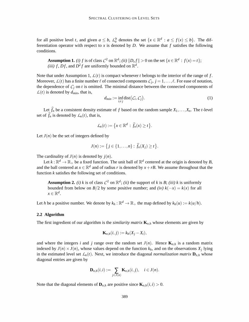
for all positive levelt, and givena ≤ b, Lba denotes the setx ∈ R
d : a ≤ f (x) ≤ b. The dif-ferentiation operator with respect tox is denoted byD. We assume thatf satisfies the followingconditions.
Assumption 1. (i) f is of classC 2 onRd; (ii) ‖Dx f‖> 0 on the setx∈Rd : f (x) = t;
(iii) f , D f , andD2 f are uniformly bounded onRd.
Note that under Assumption 1,L(t) is compact whenevert belongs to the interior of the range off .Moreover,L(t) has a finite numberℓ of connected componentsC j , j = 1, . . . , ℓ. For ease of notation,the dependence ofC j on t is omitted. The minimal distance between the connected components ofL(t) is denoted bydmin, that is,
dmin := infi 6= j
dist(Ci ,C j
). (1)
Let fn be a consistent density estimate off based on the random sampleX1, . . . ,Xn. Thet-levelset of fn is denoted byLn(t), that is,
Ln(t) :=
x∈ Rd : fn(x)≥ t
.
Let J(n) be the set of integers defined by
J(n) :=
j ∈ 1, . . . ,n : fn(Xj)≥ t.
The cardinality ofJ(n) is denoted byj(n).Let k : Rd → R+ be a fixed function. The unit ball ofRd centered at the origin is denoted byB,
and the ball centered atx∈ Rd and of radiusr is denoted byx+ rB. We assume throughout that the
functionk satisfies the following set of conditions.
Assumption 2. (i) k is of classC 2 onRd; (ii) the support ofk is B; (iii) k is uniformly
bounded from below onB/2 by some positive number; and(iv) k(−x) = k(x) for allx∈ R
d.
Let h be a positive number. We denote bykh : Rd → R+ the map defined bykh(u) := k(u/h).
2.2 Algorithm
The first ingredient of our algorithm is thesimilarity matrixKn,h whose elements are given by
Kn,h(i, j) := kh(Xj −Xi),
and where the integersi and j range over the random setJ(n). HenceKn,h is a random matrixindexed byJ(n)× J(n), whose values depend on the functionkh, and on the observationsXj lyingin the estimated level setLn(t). Next, we introduce the diagonalnormalization matrixDn,h whosediagonal entries are given by
Dn,h(i, i) := ∑j∈J(n)
Kn,h(i, j), i ∈ J(n).
Note that the diagonal elements ofDn,h are positive sinceKn,h(i, i)> 0.
389

PELLETIER AND PUDLO
The spectral clustering algorithm is based on the matrixQn,h defined by
Qn,h := D−1n,hKn,h.
Observe thatQn,h is a random Markovian transition matrix. Note also that the (random) eigenvaluesof Qn,h are real numbers and thatQn,h is diagonalizable. Indeed the matrixQn,h is conjugate to the
symmetric matrixSn,h := D−1/2n,h Kn,hD−1/2
n,h since we may write
Qn,h = D−1/2n,h Sn,hD1/2
n,h .
Moreover, the inequality‖Qn,h‖∞ ≤ 1 implies that the spectrumσ(Qn,h) is a subset of[−1;+1].Let 1= λn,1 ≥ λn,2 ≥ . . . ≥ λn, j(n) ≥ −1 be the eigenvalues ofQn,h, where in this enumeration, aneigenvalue is repeated as many times as its multiplicity.
To implement the spectral clustering algorithm, the data points of the partitioning problem arefirst embedded intoRℓ by using the eigenvectors ofQn,h associated with theℓ largest eigenvalues,namelyλn,1, λn,2, . . .λn,ℓ. More precisely, fix a collectionVn,1, Vn,2, . . . ,Vn,ℓ of such eigenvectorswith components respectively given byVn,k = Vn,k, j j∈J(n), for k= 1, . . . , ℓ. Then thej th data point,for j in J(n), is represented by the vectorρn(Xj) of the feature spaceRℓ defined byρn(Xj) :=Vn,k, j1≤k≤ℓ. At last, the embedded points are partitioned using a classical clustering method, suchas the k-means algorithm for instance.
2.3 Functional Operators Associated With the Matrices of the Algorithm
As exposed in the Introduction, some functional operators are associated with the matrices actingonC
J(n) defined in the previous paragraph. The link between matrices and functional operators isprovided by the evaluation map defined in (3) below. As a consequence, asymptotic results on theclustering algorithm may be derived by studying first the limit behavior of these operators.
To this aim, let us first introduce some additional notation. ForD a subset ofRd, let W(D)be the Banach space of complex-valued, bounded, and continuously differentiable functions withbounded gradient, endowed with the norm
‖g‖W := ‖g‖∞ +‖Dg‖∞.
Consider the non-oriented graph whose vertices are theXj ’s for j ranging inJ(n). The similaritymatrix Kn,h gives random weights to the edges of the graph and the random transition matrix Qn,h
defines a random walk on the vertices of a random graph. Associated withthis random walk is thetransition operatorQn,h : W
(Ln(t)
)→W
(Ln(t)
)defined for any functiong by
Qn,hg(x) :=∫Ln(t)
qn,h(x,y)g(y)Ptn(dy).
In this equation,Ptn is the discrete random probability measure given by
Ptn :=
1j(n) ∑
j∈J(n)
δXj ,
and
qn,h(x,y) :=kh(y−x)Kn,h(x)
, whereKn,h(x) :=∫Ln(t)
kh(y−x)Ptn(dy). (2)
390

SPECTRAL CLUSTERING ONLEVEL SETS
In the definition ofqn,h, we use the convention that 0/0= 0, but this situation does not occur in theproofs of our results.
Given theevaluation mapπn : W(Ln(t)
)→ C
j(n) defined by
πn(g) :=
g(Xj)
j∈J(n), (3)
the matrixQn,h and the operatorQn,h are related byQn,h πn = πn Qn,h. Using this relation,asymptotic properties of the spectral clustering algorithm may be deduced from the limit behaviorof the sequence of operatorsQn,hn. The difficulty, though, is thatQn,h acts onW
(Ln(t)
)andLn(t)
is a random set which varies with the sample. For this reason, we introduce asequence of operatorsQn,h acting onW
(L(t)
)and constructed fromQn,h as follows.
First of all, recall that under Assumption 1, the gradient off does not vanish on the setx ∈R
d : f (x) = t. Since f is of classC 2, a continuity argument implies that there existsε0 > 0 suchthatL t+ε0
t−ε0contains no critical points off . Under this condition, Lemma 17 states thatL(t + ε) is
diffeomorphic toL(t) for everyε such that|ε| ≤ ε0. In all of the following, it is assumed thatε0 issmall enough so that
ε0/α(ε0)< h/2, whereα(ε0) := inf‖D f (x)‖; x∈ L t
t−ε0
. (4)
Let εnn be a sequence of positive numbers such thatεn ≤ ε0 for eachn, andεn → 0 asn→ ∞. InLemma 17 an explicit diffeomorphismϕn carryingL(t) toL(t − εn) is constructed, that is,
ϕn : L(t)∼=−→ L(t − εn).
The diffeomorphismϕn induces the linear operatorΦn :W(L(t)
)→W
(L(t−εn)
)defined byΦng=
gϕ−1n .
Second, letΩn be the probability event defined by
Ωn =[‖ fn− f‖∞ ≤ εn
]∩[inf‖D fn(x)‖,x∈ L t+ε0
t−ε0
≥ 1
2‖D f‖∞
].
Note that on the eventΩn, the following inclusions hold:
L(t + εn)⊂ Ln(t)⊂ L(t − εn).
We assume that the indicator function1Ωn tends to 1 almost surely asn → ∞, which is satisfiedby common density estimatesfn under mild assumptions. For instance, consider a kernel densityestimate with a Gaussian kernel. It is a classical exercise to prove that‖ fn−E fn‖∞ converges to 0almost surely asn goes to infinity (see, e.g., Example 38 in Pollard, 1984, p. 35, or Chapter 3 inPrakasa Rao, 1983) under appropriate conditions on the bandwidth sequence. Moreover, under theconditions onf in Assumption 1, the norm of the gradient off is uniformly bounded onRd, soby using a Taylor expansion, it is easy to prove that the bias term‖E fn− f‖∞ → 0 as well. Hence‖ fn− f‖∞ → 0 almost surely. Furthermore, under Assumption 1,‖D2 f‖ is uniformly bounded onR
d so the same reasoning leads to the almost sure convergence to 0 of‖D fn −D f‖∞. Together,these facts imply that1Ωn → 1 almost surely asn→ ∞.
We are now in a position to define the operatorQn,h : W(L(t)
)→W
(L(t)
). On the eventΩn,
for all functiong in W(L(t)
), we defineQn,hg by the relation
Qn,hg(x) =1
j(n) ∑j∈J(n)
qn,h(ϕn(x),Xj)g(ϕ−1
n (Xj)), for all x∈ L(t), (5)
391

PELLETIER AND PUDLO
and we extend the definition ofQn,h to the whole probability space by setting it to the null operatoron the complementΩc
n of Ωn, that is, onΩcn, the functionQn,hg is identically zero for eachg ∈
W(L(t)
). With a slight abuse of notation, we may note thatQn,h = Φ−1
n Qn,hΦn, so that essentially,
the operatorsQn,h andQn,h are conjugate and have equal spectra, which are in turn related to thespectrum of the matrixQn,h. This is made precise in Proposition 1 below.
Proposition 1 On the eventΩn, the spectrum of the functional operator isQn,h is σ(Qn,h) = 0∪σ(Qn,h). Moreover, if ifλ 6= 0, the eigenspaces are isomorphic, that is,
πnΦn : N(Qn,h−λ)∼=−→ N(Qn,h−λ),
whereπnΦn acts on W(L(t)
)asφnΦng(x) = g
(ϕ−1
n (x)).
Proof From Equation (5), the rangeR(Qn,h) of Qn,h is spanned by the finite collection of functions
f j : L(t) → C
x 7→ qn,h(ϕn(x),Xj),
for all j ∈ J(n). Moreover, these functions form a basis ofR(Qn,h). To show this, letV be a vectorin C
J(n) such that
∑j∈J(n)
Vj f j(x) = 0 for all x∈ L(t).
By definition ofqn,h, settingy= ϕn(x), we have
∑j∈J(n)
Vjkh(y−Xj)
Kn,h(y)= 0 for all y∈ L(t − εn).
Since the support ofkh is hB, the support of the functionKn,h is equal to⋃
j∈J(n)(Xj +hB), and since
kh is positive, it follows thatVj = 0 for all j in J(n). Hence f j : j ∈ J(n) is a basis ofR(Qn,h).Now let g be an eigenfunction ofQn,h associated with an eigenvalueλ 6= 0. Then for allx in
L(t)1
j(n) ∑j∈J(n)
qn,h(ϕn(x),Xj
)g(ϕ−1
n (Xj))= λg(x). (6)
Since we consider a non-zero eigenvalue,g is in the range ofQn,h, and since the functions f j : j ∈J(n) form a basis ofR(Qn,h), there exists a unique vectorV = Vj j∈J(n) ∈ C
j(n) such that
g(x) =1
λ j(n) ∑j∈J(n)
Vjqn,h(ϕn(x),Xj), x∈ L(t).
ThereforeVj = g(ϕ−1
n (Xj))
for all j in J(n). Moreover, by evaluating (6) at anyx= ϕ−1n (Xi) with
i ∈ J(n),
∑j∈J(n)
qn,h(Xi ,Xj
)g(ϕ−1
n (Xj))= λg
(ϕ−1
n (Xi)),
which implies thatQn,hV = λV. Consequently,V is an eigenvector ofQn,h associated with theeigenvalueλ. Hence
σ(Qn,h)⊂ σ(Qn,h)∪0, (7)
392
SPECTRAL CLUSTERING ONLEVEL SETS
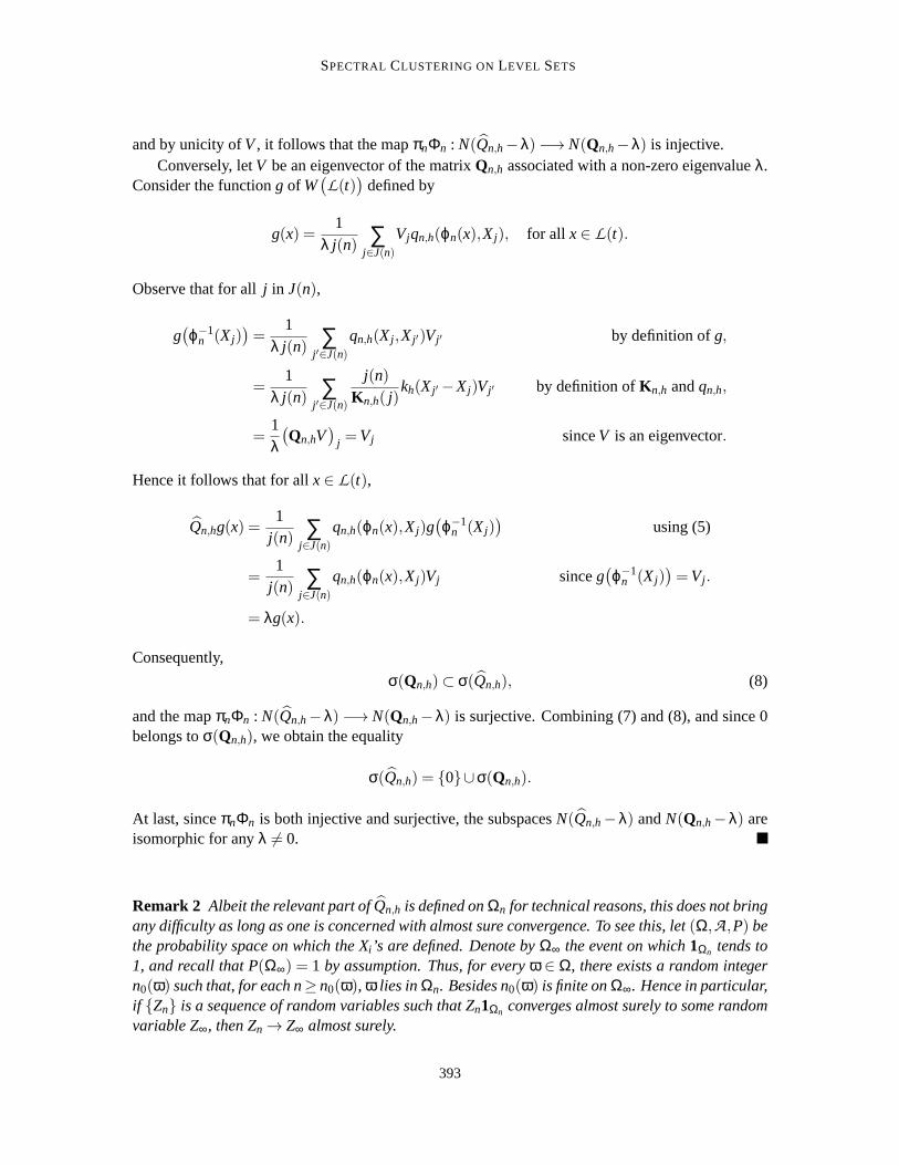
and by unicity ofV, it follows that the mapπnΦn : N(Qn,h−λ)−→ N(Qn,h−λ) is injective.Conversely, letV be an eigenvector of the matrixQn,h associated with a non-zero eigenvalueλ.
Consider the functiong of W(L(t)
)defined by
g(x) =1
λ j(n) ∑j∈J(n)
Vjqn,h(ϕn(x),Xj), for all x∈ L(t).
Observe that for allj in J(n),
g(ϕ−1
n (Xj))=
1λ j(n) ∑
j ′∈J(n)
qn,h(Xj ,Xj ′)Vj ′ by definition ofg,
=1
λ j(n) ∑j ′∈J(n)
j(n)Kn,h( j)
kh(Xj ′ −Xj)Vj ′ by definition ofKn,h andqn,h,
=1λ(Qn,hV
)j =Vj sinceV is an eigenvector.
Hence it follows that for allx∈ L(t),
Qn,hg(x) =1
j(n) ∑j∈J(n)
qn,h(ϕn(x),Xj)g(ϕ−1
n (Xj))
using (5)
=1
j(n) ∑j∈J(n)
qn,h(ϕn(x),Xj)Vj sinceg(ϕ−1
n (Xj))=Vj .
= λg(x).
Consequently,
σ(Qn,h)⊂ σ(Qn,h), (8)
and the mapπnΦn : N(Qn,h−λ)−→ N(Qn,h−λ) is surjective. Combining (7) and (8), and since 0belongs toσ(Qn,h), we obtain the equality
σ(Qn,h) = 0∪σ(Qn,h).
At last, sinceπnΦn is both injective and surjective, the subspacesN(Qn,h−λ) andN(Qn,h−λ) areisomorphic for anyλ 6= 0.
Remark 2 Albeit the relevant part ofQn,h is defined onΩn for technical reasons, this does not bringany difficulty as long as one is concerned with almost sure convergence. To see this, let(Ω,A ,P) bethe probability space on which the Xi ’s are defined. Denote byΩ∞ the event on which1Ωn tends to1, and recall that P(Ω∞) = 1 by assumption. Thus, for everyω ∈ Ω, there exists a random integern0(ω) such that, for each n≥ n0(ω), ω lies inΩn. Besides n0(ω) is finite onΩ∞. Hence in particular,if Zn is a sequence of random variables such that Zn1Ωn converges almost surely to some randomvariable Z∞, then Zn → Z∞ almost surely.
393

PELLETIER AND PUDLO
3. Operator Norm Convergence
In this section, we start by establishing the uniform convergence of an unnormalized empiricalfunctional operator. The main operator norm convergence result (Theorem 4) is stated in Section 3.2.The proofs of these theorems rely on several auxiliary lemmas which are stated and proved inSection 5.
3.1 Unnormalized Operators
Let r : L(t − ε0)×Rd → R be a given function. Define the linear operatorsRn andR onW
(L(t)
)
respectively by
Rng(x) :=∫Ln(t)
r(ϕn(x),y
)g(ϕ−1
n (y))P
tn(dy), and Rg(x) :=
∫L(t)
r(x,y)g(y)µt(dy).
Proposition 3 Assume the following conditions on the function r:(i) r is continuously differentiable with compact support ;(ii) r is uniformly bounded onL(t − ε0)×R
d, that is,‖r‖∞ < ∞ ;(iii) the differential Dxr of the function r with respect to x is uniformly bounded onL(t − ε0)×R
d,that is,‖Dxr‖∞ := sup
‖Dxr(x,y)‖ : (x,y) ∈ L(t − ε0)×R
d< ∞.
Then, as n→ ∞,sup∥∥Rng−Rg
∥∥∞ : ‖g‖W ≤ 1
→ 0 almost surely.
The key argument for proving Proposition 3 is that the collection of functions
y 7→ r(x,y)g(y)1L(t)(y) : x∈ L(t), ‖g‖W(L(t)) ≤ 1
is Glivenko-Cantelli, which is proved in Lemma 13. Let us recall that a collectionF of functions issaid to be Glivenko-Cantelli, or to satisfy a uniform law of large number, if
supg∈F
∣∣∣∣∣1n
n
∑i=1
g(Xi)−E[X]
∣∣∣∣∣→ 0 almost surely,
whereX,X1,X2, . . . are i.i.d. random variables.Proof In all this proof, we shall use the following convention: given a functiong defined only onsome subsetD of Rd, for any subsetA ⊂D, and anyx∈R
d, the notationg(x)1A(x) stands forg(x)is x∈ A and for 0 otherwise. Set
Sng(x) :=1
µ(L(t))1n
n
∑i=1
r(ϕn(x),Xi
)g(ϕ−1
n (Xi))1Ln(t)(Xi),
Tng(x) :=1
µ(L(t)
) 1n
n
∑i=1
r(ϕn(x),Xi
)g(Xi)1L(t)(Xi),
Ung(x) :=1
µ(L(t)
) 1n
n
∑i=1
r(x,Xi
)g(Xi)1L(t)(Xi).
and consider the inequality∣∣Rng(x)−Rg(x)
∣∣≤∣∣Rng(x)−Sng(x)
∣∣+∣∣Sng(x)−Tng(x)
∣∣+∣∣Tng(x)−Ung(x)
∣∣+∣∣Ung(x)−Rg(x)
∣∣, (9)
394

SPECTRAL CLUSTERING ONLEVEL SETS
for all x∈ L(t) and allg∈W(L(t)
).
The first term in (9) is bounded uniformly by
∣∣Rng(x)−Sng(x)∣∣≤∣∣∣∣
nj(n)
− 1
µ(L(t)
)∣∣∣∣‖r‖∞‖g‖∞
and sincej(n)/n tends toµ(L(t)) almost surely asn→ ∞, we conclude that
sup∥∥Rng−Sng
∥∥∞ : ‖g‖W ≤ 1
→ 0 a.s. asn→ ∞. (10)
For the second term in (9), we have
|Sng(x)−Tng(x)| ≤ ‖r‖∞
µ(L(t)
) 1n
n
∑i=1
∣∣g(ϕ−1
n (Xi))1Ln(t)(Xi)−g(Xi)1L(t)(Xi)
∣∣
=‖r‖∞
µ(L(t)
) 1n
n
∑i=1
gn(Xi), (11)
wheregn is the function defined on the whole spaceRd by
gn(x) =∣∣∣g(ϕ−1
n (x))1Ln(t)(x)−g(x)1L(t)(x)
∣∣∣.
Consider the partition ofRd given byRd = B1,n∪B2,n∪B3,n∪B4,n, where
B1,n := Ln(t)∩L(t), B2,n := Ln(t)∩L(t)c,B3,n := Ln(t)c∩L(t), B4,n := Ln(t)c∩L(t)c.
The sum overi in (11) may be split into four parts as
1n
n
∑i=1
gn(Xi) = I1(x,g)+ I2(x,g)+ I3(x,g)+ I4(x,g) (12)
where
Ik(x,g) :=1n
n
∑i=1
gn(Xi)1Xi ∈ Bk,n.
First, I4,n(x,g) = 0 sincegn is identically 0 onB4,n. Second,
I2(x,g)+ I3(x,g)≤ ‖g‖∞1n
n
∑i=1
1L(t)∆Ln(t)(Xi) (13)
Applying Lemma 11 together with the almost sure convergence of1Ωn to 1, we obtain that
1n
n
∑j=1
1L(t)∆Ln(t)(Xj)→ 0 almost surely. (14)
Third,
I1(x,g)≤ supx∈L(t)
∣∣∣∣g(ϕ−1
n (x))−g(x)
∣∣∣∣≤ ‖Dxg‖∞ supx∈L(t)
‖ϕ−1n (x)−x‖
≤ ‖Dxg‖∞ supx∈L(t)
‖x−ϕn(x)‖→ 0 (15)
395

PELLETIER AND PUDLO
asn→ ∞ by Lemma 17. Thus, combining (11), (12), (13), (14) and (15) leads to
sup∥∥Sng−Tng
∥∥∞ : ‖g‖W ≤ 1
→ 0 a.s. asn→ ∞. (16)
For the third term in (9), using the inequality∣∣r(ϕn(x),Xi
)− r(x,Xi
)∣∣≤ ‖Dxr‖∞ supx∈L(t)
‖ϕn(x)−x‖
we deduce that∣∣Tng(x)−Ung(x)
∣∣≤ 1
µ(L(t)
)‖g‖∞‖Dxr‖∞ supx∈L(t)
‖ϕn(x)−x‖.
and sosup∥∥Tng−Ung
∥∥∞ : ‖g‖W ≤ 1
→ 0 a.s. asn→ ∞, (17)
by Lemma 17.At last, for the fourth term in (9), we conclude by Lemma 13 that
sup∥∥Ung−Rg
∥∥∞ : ‖g‖W ≤ 1
→ 0 a.s. asn→ ∞.
Finally, reporting (10), (16) and (17) in (9) yields the desired result.
3.2 Normalized Operators
Theorem 4 states thatQn,h converges in operator norm to the limit operatorQh : W(L(t)
)→
W(L(t)
)defined by
Qhg(x) =∫L(t)
qh(x,y)g(y)µt(dy), (18)
whereµt denotes the conditional distribution ofX given the event[X ∈ L(t)
], and where
qh(x,y) =kh(y−x)
Kh(x), with Kh(x) =
∫L(t)
kh(y−x)µt(dy). (19)
Theorem 4 (Operator Norm Convergence) Suppose that Assumptions 1 and 2 hold. We have∥∥Qn,h−Qh
∥∥W → 0 almost surely as n→ ∞.
Proof We will prove that, asn→ ∞, almost surely,
sup
∥∥∥Qn,hg−Qhg∥∥∥
∞: ‖g‖W ≤ 1
→ 0 (20)
and
sup
∥∥∥Dx[Qn,hg
]−Dx
[Qhg
]∥∥∥∞
: ‖g‖W ≤ 1
→ 0 (21)
To this aim, we introduce the operatorQn,h acting onW(L(t)) as
Qn,hg(x) =∫Ln(t)
qh(ϕn(x),y)g(ϕ−1
n (y))P
tn(dy).
396

SPECTRAL CLUSTERING ONLEVEL SETS
Proof of (20) For all g∈W(L(t)
), we have
∥∥Qn,hg−Qhg∥∥
∞ ≤∥∥Qn,hg− Qn,hg
∥∥∞ +
∥∥Qn,hg−Qhg∥∥
∞. (22)
First, by Lemma 14, the functionr = qh satisfies the condition in Proposition 3, so that
sup‖Qn,hg−Qhg‖∞ : ‖g‖W ≤ 1
→ 0 (23)
with probability one asn→ ∞.Next, since‖qh‖∞ < ∞ by Lemma 14, there exists a finite constantCh such that,
‖Qn,hg‖∞ ≤Ch for all n and allg with ‖g‖W ≤ 1. (24)
By definition ofqn,h, for all x,y in the level setL(t), we have
qn,h(x,y) =Kh(x)
Kn,h(x)qh(x,y).
So
∣∣∣Qn,hg(x)− Qn,hg(x)∣∣∣=∣∣∣∣∣
Kn(ϕn(x)
)
Kn,h(ϕn(x)
) −1
∣∣∣∣∣∣∣∣Qn,hg(x)
∣∣∣
≤Ch supx∈L(t)
∣∣∣∣∣Kn(ϕn(x)
)
Kn,h(ϕn(x)
) −1
∣∣∣∣∣ ,
whereCh is as in (24). Applying Lemma 16 yields
sup‖Qn,hg− Qn,hg‖∞ : ‖g‖W ≤ 1
→ 0 (25)
with probability one asn→ ∞. Reporting (23) and (25) in (22) proves (20).
Proof of (21) We have∥∥∥∥Dx
[Qn,hg
]−Dx
[Qhg
]∥∥∥∥∞≤∥∥∥∥Dx
[Qn,hg
]−Dx
[Qhg
]∥∥∥∥∞+
∥∥∥∥Dx
[Qn,hg
]−Dx
[Qhg
]∥∥∥∥∞. (26)
The second term in right han side of (26) is bounded by∥∥∥∥Dx
[Qn,hg
]−Dx
[Qhg
]∥∥∥∥∞≤∥∥Dxϕn
∥∥∞
∥∥Rng−Rg∥∥
∞,
where
Rng(x) :=∫Ln(t)
(Dxqh)(ϕn(x),y)g(ϕ−1
n (y))P
tn(dy) and
Rg(x) :=∫L(t)
(Dxqh)(ϕn(x),y)g(ϕ−1
n (y))µt(dy).
397

PELLETIER AND PUDLO
By lemma 17,x 7→ Dxϕn(x) converges to the identity matrixId of Rd, uniformly in x overL(t). So‖Dxϕn(x)‖ is bounded by some finite constantCϕ uniformly overn andx∈ L(t) and
∥∥∥∥Dx
[Qn,hg
]−Dx
[Qhg
]∥∥∥∥∞≤Cϕ
∥∥Rng−Rg∥∥
∞.
By Lemma 14, the mapr : (x,y) 7→Dxqh(x,y) satisfies the conditions in Proposition 3. Thus,‖Rng−Rg‖∞ converges to 0 almost surely, uniformly overg in the unit ball ofW(L(t)), and we deduce that
sup
∥∥∥∥Dx
[Qn,hg
]−Dx
[Qhg
]∥∥∥∥∞
: ‖g‖W ≤ 1
→ 0 a.s. asn→ ∞. (27)
For the first term in right hand side of (26), observe first that there exists a constantC′h such that,
for all n and allg in the unit ball ofW(L(t)
),
‖Rn,hg‖∞ ≤C′h, for all n and allg with ‖g‖W ≤ 1, (28)
by Lemma 14.On the one hand, we have
Dx[qn,h(ϕn(x),y)
]=
Kh(ϕn(x)
)
Kn,h(ϕn(x)
)Dxϕn(x)(Dxqh)(ϕn(x),y
)+Dx
[Kh(ϕn(x)
)
Kn,h(ϕn(x)
)]
qh(ϕn(x),y
).
Hence,
Dx
[Qn,hg(x)
]=
Kh(ϕn(x)
)
Kn,h(ϕn(x)
)Dxϕn(x)Rng(x)+Dx
[Kh(ϕn(x)
)
Kn,h(ϕn(x)
)]
Qn,hg(x).
On the other hand, sinceDx[qh(ϕn(x),y
)]= Dxϕn(x)(Dxqh)
(ϕn(x),y
),
Dx
[Qn,hg(x)
]= Dxϕn(x)Rng(x).
Thus,
Dx
[Qn,hg(x)
]−Dx
[Qhg(x)
]=Dx
[Kh(ϕn(x)
)
Kn,h(ϕn(x)
)]
Qn,hg(x)+
(Kh(ϕn(x)
)
Kn,h(ϕn(x)
) −1
)Dxϕn(x)Rng(x).
Using the Inequalities (24) and (28), we obtain
∥∥∥Dx
[Qn,hg
]−Dx
[Qhg
]∥∥∥∞≤Ch sup
x∈L(t)
∣∣∣∣∣Dx
[Kh(ϕn(x)
)
Kn,h(ϕn(x)
)]∣∣∣∣∣+C′
hCϕ supx∈L(t)
∣∣∣∣∣Kh(ϕn(x)
)
Kn,h(ϕn(x)
) −1
∣∣∣∣∣ .
and by applying Lemma 16, we deduce that
sup
∥∥∥∥Dx
[Qn,hg
]−Dx
[Qhg
]∥∥∥∥∞
: ‖g‖W ≤ 1
→ 0 a.s. asn→ ∞. (29)
Reporting (27) and (29) in (26) proves (21).
398
SPECTRAL CLUSTERING ONLEVEL SETS
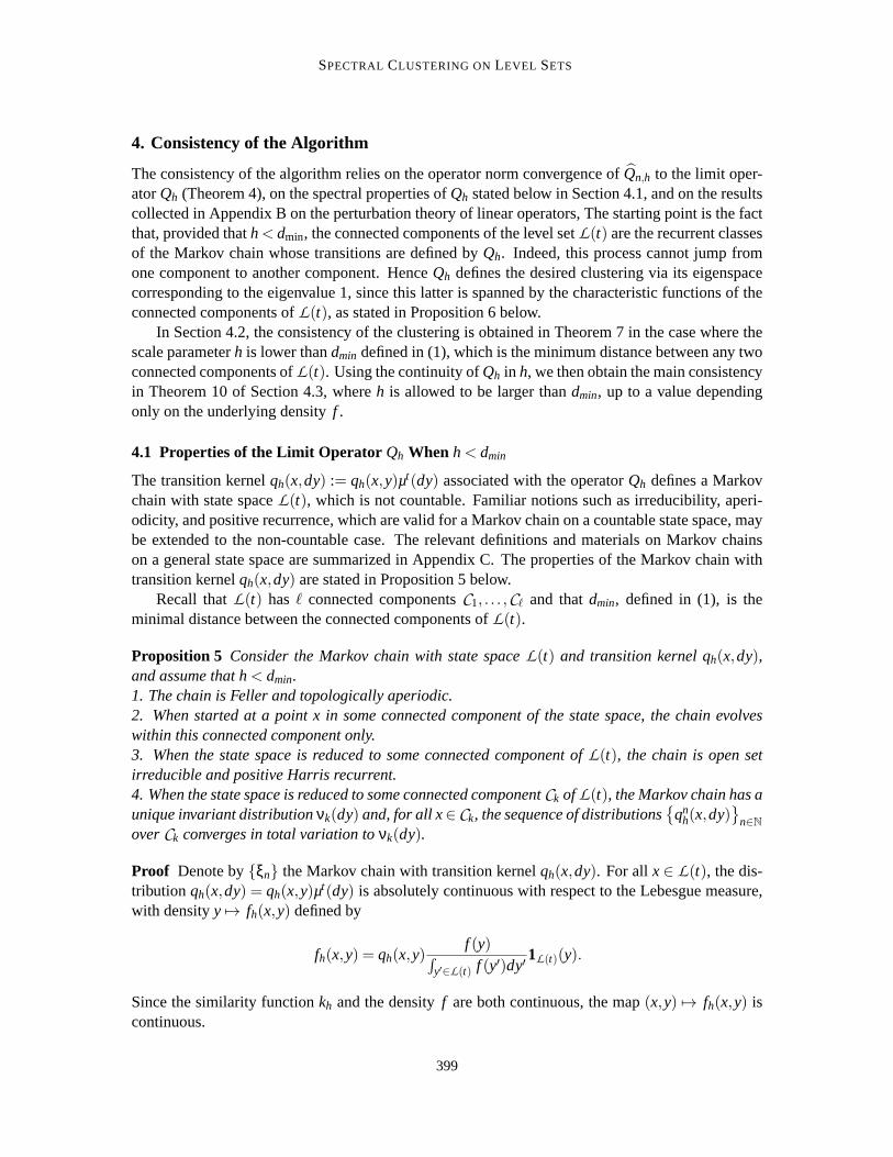
4. Consistency of the Algorithm
The consistency of the algorithm relies on the operator norm convergence of Qn,h to the limit oper-atorQh (Theorem 4), on the spectral properties ofQh stated below in Section 4.1, and on the resultscollected in Appendix B on the perturbation theory of linear operators, Thestarting point is the factthat, provided thath< dmin, the connected components of the level setL(t) are the recurrent classesof the Markov chain whose transitions are defined byQh. Indeed, this process cannot jump fromone component to another component. HenceQh defines the desired clustering via its eigenspacecorresponding to the eigenvalue 1, since this latter is spanned by the characteristic functions of theconnected components ofL(t), as stated in Proposition 6 below.
In Section 4.2, the consistency of the clustering is obtained in Theorem 7 in thecase where thescale parameterh is lower thandmin defined in (1), which is the minimum distance between any twoconnected components ofL(t). Using the continuity ofQh in h, we then obtain the main consistencyin Theorem 10 of Section 4.3, whereh is allowed to be larger thandmin, up to a value dependingonly on the underlying densityf .
4.1 Properties of the Limit Operator Qh When h< dmin
The transition kernelqh(x,dy) := qh(x,y)µt(dy) associated with the operatorQh defines a Markovchain with state spaceL(t), which is not countable. Familiar notions such as irreducibility, aperi-odicity, and positive recurrence, which are valid for a Markov chain ona countable state space, maybe extended to the non-countable case. The relevant definitions and materials on Markov chainson a general state space are summarized in Appendix C. The properties ofthe Markov chain withtransition kernelqh(x,dy) are stated in Proposition 5 below.
Recall thatL(t) hasℓ connected componentsC1, . . . ,Cℓ and thatdmin, defined in (1), is theminimal distance between the connected components ofL(t).
Proposition 5 Consider the Markov chain with state spaceL(t) and transition kernel qh(x,dy),and assume that h< dmin.1. The chain is Feller and topologically aperiodic.2. When started at a point x in some connected component of the state space, the chain evolveswithin this connected component only.3. When the state space is reduced to some connected component ofL(t), the chain is open setirreducible and positive Harris recurrent.4. When the state space is reduced to some connected componentCk ofL(t), the Markov chain has aunique invariant distributionνk(dy) and, for all x∈ Ck, the sequence of distributions
qn
h(x,dy)
n∈NoverCk converges in total variation toνk(dy).
Proof Denote byξn the Markov chain with transition kernelqh(x,dy). For allx∈ L(t), the dis-tribution qh(x,dy) = qh(x,y)µt(dy) is absolutely continuous with respect to the Lebesgue measure,with densityy 7→ fh(x,y) defined by
fh(x,y) = qh(x,y)f (y)∫
y′∈L(t) f (y′)dy′1L(t)(y).
Since the similarity functionkh and the densityf are both continuous, the map(x,y) 7→ fh(x,y) iscontinuous.
399

PELLETIER AND PUDLO
Now, by induction onn, the distribution ofξn conditioned byξ0 = x, which isqn+1h (x,dy) is also
absolutely continuous with respect to the Lebesgue measure and its densityy 7→ f nh (x,y) satisfies
f nh (x,y) =
∫z∈L(t)
f n−1h (x,z) fh(z,y)dz=
∫z∈L(t)
fh(x,z) f n−1h (z,y)dz, (30)
where the last equality follows from the Markov property. Moreover, one easily sees by inductionthat the map(x,y) 7→ f n
h (x,y) is continuous.1. Since the similarity functionkh is continuous, with compact supporthB, the map
x 7→ Qhg(x) =∫L(t)
qh(x,dy)g(y)
is continuous for every bounded, measurable functiong. Hence, the chain is Feller.Now we have to prove that the chain is topologically aperiodic, that is, thatqn
h(x,x+ηB) > 0for eachx ∈ L(t), for all n ≥ 1 andη > 0, whereqn
h(x, ·) is the distribution ofξn conditioned onξ0 = x. Since the distributionqn
h(x, ·) admits a continuous densityf nh (x, ·), it is enough to prove that
f nh (x,x) > 0. Sincekh is bounded from below on(h/2)B by Assumption 2, the densityfh(x,y) is
strictly positive for ally∈ x+hB/2. By induction overn, using (30),f nh (x,x) > 0 and the chain is
topologically aperiodic.
2. Without loss of generality, since the numbering of the connected components is arbitrary, assumethatx∈ C1. Let y be a point ofL(t) which does not belong toC1. Then‖y−x‖ ≥ dmin > h so thatqh(x,y) = 0. Whence,
Px(ξ1 ∈ C1) = qh(x,C1) =∫C1
qh(x,y)µt(dy) =
∫L(t)
qh(x,y)µt(dy) = 1.
3. Assume that the state space is reduced toC1. In order to prove that the chain is open set irre-ducible, it is enough to prove that, for eachx,y∈ C1 andη > 0, there exists some integerN such thatPx(ξN ∈ y+ηB) = qN
h (x,y+ηB) is positive. Observe thatqnh(x,dy) is the distribution with density
qnh(x,y) =
∫x1,...,xn−1∈C1
qh(x,x1)qh(x1,x2) . . .qh(xn−1,y)dx1dx2dxn−1
and(x1, . . . ,xn−1) 7→ qh(x,x1)qh(x1,x2) . . .qh(xn−1,y) is continuous. Hence, it is enough to provethat there exists some integerN and a finite sequencex1, . . .xN such that
qh(x,x1)qh(x1,x2) . . .qh(xN−1,y)> 0.
SinceC1 is connected, there exists a finite sequencex0, x1, . . .xN of points inC1 such thatx0 = x,xN = y, and‖xi −xi+1‖ ≤ h/2 for eachi. Therefore
qh(x,x1)qh(x1,x2) . . .qh(xN−1,y)> 0
which proves that the chain is open set irreducible.SinceC1 is compact, the chain is non-evanescent, and so it is Harris recurrent. Recall that
k(x) = k(−x) from Assumption 2. Thereforekh(y−x) = kh(x−y) which yields
Kh(x)qh(x,dy)µt(dx) = Kh(y)qh(y,dx)µt(dy).
400
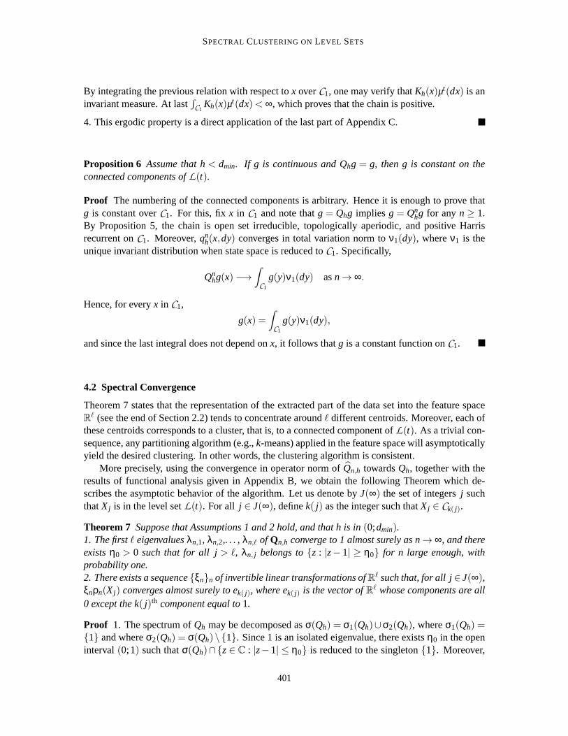
SPECTRAL CLUSTERING ONLEVEL SETS
By integrating the previous relation with respect tox overC1, one may verify thatKh(x)µt(dx) is aninvariant measure. At last
∫C1
Kh(x)µt(dx)< ∞, which proves that the chain is positive.
4. This ergodic property is a direct application of the last part of Appendix C.
Proposition 6 Assume that h< dmin. If g is continuous and Qhg = g, then g is constant on theconnected components ofL(t).
Proof The numbering of the connected components is arbitrary. Hence it is enough to prove thatg is constant overC1. For this, fixx in C1 and note thatg = Qhg implies g = Qn
hg for any n ≥ 1.By Proposition 5, the chain is open set irreducible, topologically aperiodic,and positive Harrisrecurrent onC1. Moreover,qn
h(x,dy) converges in total variation norm toν1(dy), whereν1 is theunique invariant distribution when state space is reduced toC1. Specifically,
Qnhg(x)−→
∫C1
g(y)ν1(dy) asn→ ∞.
Hence, for everyx in C1,
g(x) =∫C1
g(y)ν1(dy),
and since the last integral does not depend onx, it follows thatg is a constant function onC1.
4.2 Spectral Convergence
Theorem 7 states that the representation of the extracted part of the data set into the feature spaceRℓ (see the end of Section 2.2) tends to concentrate aroundℓ different centroids. Moreover, each of
these centroids corresponds to a cluster, that is, to a connected component ofL(t). As a trivial con-sequence, any partitioning algorithm (e.g.,k-means) applied in the feature space will asymptoticallyyield the desired clustering. In other words, the clustering algorithm is consistent.
More precisely, using the convergence in operator norm ofQn,h towardsQh, together with theresults of functional analysis given in Appendix B, we obtain the following Theorem which de-scribes the asymptotic behavior of the algorithm. Let us denote byJ(∞) the set of integersj suchthatXj is in the level setL(t). For all j ∈ J(∞), definek( j) as the integer such thatXj ∈ Ck( j).
Theorem 7 Suppose that Assumptions 1 and 2 hold, and that h is in(0;dmin).1. The firstℓ eigenvaluesλn,1, λn,2,. . . ,λn,ℓ of Qn,h converge to 1 almost surely as n→ ∞, and thereexistsη0 > 0 such that for all j> ℓ, λn, j belongs toz : |z− 1| ≥ η0 for n large enough, withprobability one.2. There exists a sequenceξnn of invertible linear transformations ofRℓ such that, for all j∈ J(∞),ξnρn(Xj) converges almost surely to ek( j), where ek( j) is the vector ofRℓ whose components are all0 except the k( j)th component equal to1.
Proof 1. The spectrum ofQh may be decomposed asσ(Qh) = σ1(Qh)∪σ2(Qh), whereσ1(Qh) =1 and whereσ2(Qh) = σ(Qh)\1. Since 1 is an isolated eigenvalue, there existsη0 in the openinterval (0;1) such thatσ(Qh)∩z∈ C : |z−1| ≤ η0 is reduced to the singleton1. Moreover,
401
PELLETIER AND PUDLO
1 is an eigenvalue ofQh of multiplicity ℓ, by Proposition 6. Hence by Theorem 18,W(L(t)
)
decomposes intoW(L(t)
)= M1⊕M2 whereM1 = N(Qh−1) andM2 is mapped into itself byQh.
Split the spectrum ofQn,h asσ(Qn,h
)= σ1
(Qn,h
)∪σ2
(Qn,h
), where
σ1(Qn,h
)= σ
(Qn,h
)∩
z∈ C : |z−1|< η0.
By Theorem 18, this decomposition of the spectrum ofQn,h yields a decomposition ofW(L(t)
)as
W(L(t)
)= Mn,1⊕Mn,2, whereMn,1 andMn,2 are stable subspaces underQn,h and
Mn,1 :=⊕
λ∈σ1(Qn,h)
N(Qn,h−λ).
By Proposition 1,σ(Qn,h) = σ(Qn,h)∪0. Statement 6 of Theorem 19 implies that, for alln largeenough, the total multiplicity of the eigenvalues inσ1(Qn,h) is dim(M1) = dim(N(Qh − 1)) = ℓ.Hence, for allj > ℓ, λn, j belongs toz : |z−1| ≥ η0. Moreover, statement 4 of Theorem 19 provesthat the firstℓ eigenvalues converges to 1.2. In addition to the convergence of the eigenvalues ofQn,h, the convergence of the eigenspaces alsoholds. More precisely, letΠ be the projector onM1 = N(Qh−1) alongM2 andΠn the projector onMn,1 alongMn,2. Statements 2, 3, 5 and 6 of Theorem 19 leads to
‖Πn−Π‖W → 0 a.s. (31)
and the dimension ofMn,1 is equal toℓ for all n large enough.Denote byEn,1 the subspace ofC j(n) spanned by the eigenvectors ofQn,h corresponding to the
eigenvaluesλn,1, . . .λn,ℓ. Since
Mn,1 =⊕
λ∈σ1(Qn,h)
N(Qn,h−λ) and En,1 =⊕
λ∈σ1(Qn,h)
N(Qn,h−λ),
by Proposition 1 the mapπnΦn induces an isomorphism betweenMn,1 and En,1. Moreover,Πn
induces a morphismΠn from M1 to Mn,1 which converges to the identity map ofM1 in W-norm by(31). Hence, ifn is large enough,Πn is invertible and we have the following isomorphisms of vectorspaces:
Πn : M1∼=−→ Mn,1 and πnΦn : Mn,1
∼=−→ En,1. (32)
By Proposition 6, the functionsgk := 1Ck, k= 1,2. . . , ℓ, form a basis ofM1 = N(Qh−1). Usingthe isomorphisms of (32), we may define for allk∈ 1, . . . ℓ,
gn,k := Πngk, and ϑn,k := πnΦngn,k = πnΦnΠngk.
Then the collectionsgn,kk=1,...,ℓ andϑn,kk=1,...,ℓ are a basis ofMn,1 andEn,1 respectively. More-over, for allk∈ 1, . . . , ℓ, gn,k converges to1Ck in W-norm by (31). And, asn→ ∞, if j ∈ J(∞),
ϑn,k, j = Πn(1Ck)ϕ−1n (Xj)→ 1Ck(Xj) =
1 if k= k( j),
0 otherwise.(33)
402

SPECTRAL CLUSTERING ONLEVEL SETS
The eigenvectorsVn,1, . . . ,Vn,ℓ chosen in the algorithm form another basis ofEn,1. Hence, thereexists a matrixξn of dimensionℓ× ℓ such that
ϑn,k =ℓ
∑i=1
ξn,k,i Vn,i .
Hence thej th component ofϑn,k, for all j ∈ J(n), may be expressed as
ϑn,k, j =ℓ
∑i=1
ξn,k,i Vn,i, j .
Sinceρn(Xj) is the vector ofRℓ with componentsVn,i, ji=1,...,ℓ, the vectorϑn,•, j = ϑn,k, jk of Rℓ
is related toρn(Xj) by the linear transformationξn, that is,
ϑn,•, j = ξn ρn(Xj).
The convergence ofϑn,•, j to ek( j) then follows from (33) and Theorem 7 is proved.
Remark 8 The last step of the spectral clustering algorithm consists in partitioning the transformeddata in the feature space, which can be performed by a standard clusteringalgorithm, like the k-means algorithm or a hierarchical clustering. Theorem 7 states that thereexists a choice for a basisof ℓ eigenvectors such that the transformed data concentrates on theℓ canonical basis vectors ek ofRℓ. Consequently, upon choosing a suitable collection Vn,1, . . . ,Vn,ℓ of eigenvectors, for anyε > 0,
with probability one, for n large enough, the transformed dataρn(Xj)’s belong to the union of ballscentered at e1, . . . ,eℓ and of radiusε. Combining this result with known asymptotic properties of theaforementioned clustering algorithms leads to the desired partition.
For instance, a hierarchical agglomerative method with single linkage allowsto separate groupsprovided that the minimal distance between the groups is larger than the maximal diameter of thegroups. In the preceding display, by choosingε such that2ε <
√2, with probability one for n large
enough the points belong toℓ balls of diameter2ε which are all at a distance strictly larger than2ε.Consequently, cutting the dendrogram tree of the single linkage hierarchical clustering at a height2ε will correctly separate the groups, and the algorithm is consistent.
Similarly, for the k-means algorithm, we may note that, upon choosing a suitable basis of eigen-vectors, the empirical measure associated with the transformed data converges to a discrete mea-sure supported by the canonical vectors e1, . . . ,eℓ. Consistency of the grouping then follows fromthe well-known properties of the vector quantization method; see Pollard (1981).
The existence of an appropriate choice of eigenvectors is guaranteed by Theorem 7. How tochoose such a collection of eigenvectors in practice is left for future research. In this direction,we may note that the two clustering methods considered above (i.e., k-means and hierarchical)are invariant by isometries. So the main question concerns the choice of the normalization of anarbitrary collection of eigenvectors.
Remark 9 Note that if one is only interested in the consistency property, then this resultcould beobtained through another route. Indeed, it is shown in Biau et al. (2007)that the neighborhoodgraph with connectivity radius h has asymptotically the same number of connected components as
403

PELLETIER AND PUDLO
the level set. Hence, splitting the graph into its connected components leads tothe desired clusteringas well. But Theorem 7, by giving the asymptotic representation of the data when embedded in thefeature spaceRℓ, provides additional insight into spectral clustering algorithms. In particular,Theorem 7 provides a rationale for the heuristic of Zelnik-Manor and Perona (2004) for automaticselection of the number of groups. Their idea is to quantify the amount of concentration of thepoints embedded in the feature space, and to select the number of groupsleading to the maximalconcentration. Their method compared favorably with the eigengap heuristic considered in vonLuxburg (2007).
4.3 Further Spectral Convergence
Naturally, the selection of the number of groups is also linked with the choice ofthe parameterh. In this direction, let us emphasize that the operatorsQn,h andQh depend continuously on thescale parameterh. Thus, the spectral properties of both operators will be close to the onesstated inTheorem 7 ifh is in a neighborhood of the interval(0;dmin). This follows from the continuity ofan isolated set of eigenvalues, as stated in Appendix B. In particular, the sum of the eigenspaces ofQh associated with the eigenvalues close to 1 is spanned by functions that are close to (inW(L(t))-norm) the characteristic functions of the connected components ofL(t). Hence, the representationof the data set in the feature spaceR
ℓ still concentrates on some neighborhoods ofek, 1≤ k≤ ℓ anda simple clustering algorithm such as thek-means algorithm will still lead to the desired partition.This is made precise in the following Theorem.
Theorem 10 Suppose that assumptions 1 and 2 hold. There exists hmax> dmin which depends onlyon the density f , such that, for any h∈ (0;hmax), the event “for all n large enough, the representationof the extracted data set in the feature space, namelyρn(Xj) j∈J(n), concentrates inℓ cubes ofRℓ
that do not overlap” has probability one. Moreover, on this event of probability one, theℓ cubesare in one-to-one correspondence with theℓ connected component ofL(t). Hence, for all n largeenough, eachρn(Xj) with j ∈ J(∞) is in the cube corresponding to the k( j)th cluster for all n largeenough.
This result contrasts with the graph techniques used to recover the connected components, as in,for example, Biau et al. (2007), where an unweighted graph is defined by connecting two observa-tions if and only if their distance is smaller thanh. The partition is then obtained by the connectedcomponents of the graph. However, whenh is taken slightly larger than the critical valuedmin, atleast two connected components cannot be separated using the graph partitioning algorithm.Proof Let us begin with the following consequence of Proposition 6. For allh≤ dmin theℓ largesteigenvalues ofQh are all equal to 1 and the corresponding eigenspace is spanned by the indicatorfunctions of the connected components of thet-level set. Moreover, 1 is an isolated eigenvalue ofQdmin, that is, there existsη0 in the interval(0;1) such thatσ(Qdmin)∩z∈ C : |z−1| < η0 is thesingleton1.
We choose an arbitrary constantC0 in (0;1/2). Sinceh 7→ Qh is continuous for the topology ofthe operator norm, Theorem 19 implies that there exists a neighborhood(hmin;hmax) of dmin suchthat, for allh in (hmin;hmax),(i) Qh has exactlyℓ eigenvalues inz∈ C : |z−1|< η0;(ii) the sum of the corresponding eigenspaces ofQh is spanned byℓ functions, sayg1, . . . ,gℓ, atdistance (in‖ · ‖W-norm) less thanC0/2 from the indicator functions of the connected components
404

SPECTRAL CLUSTERING ONLEVEL SETS
of L(t) :‖gk−1Ck‖∞ ≤ ‖gk−1Ck‖W <C0/2 for k= 1, . . . , ℓ. (34)
Now, fix h in (dmin;hmax). We follow the arguments leading to Theorem 7. The convergence in(33) becomes
limn→∞
ϑn,k, j = gk(Xj) almost surely.
Hence, there existsn0 such that, for alln ≥ n0, j ∈ J(n) and k ∈ 1, . . . , ℓ, we have|ϑn,k, j −gk(Xj)| < C0/2. With the triangular inequality and (34), we obtain|ϑn,k, j − 1Ck(Xj)| < C0, that is,the representation of the extracted data set in the feature space concentrates in cubes with edgelength 2C0, centered atek, k = 1, . . . , ℓ, up to a linear transformation ofRℓ, for all n large enough.Moreover, ifXj with j ∈ J(∞) lies in Ck( j), then its representation is in the cube centered atek( j).Since those cubes have edge length 2C0 < 1, they do not overlap. Hence, a classical method such asthe k-means algorithm will asymptotically partition the extracted data set as desired.
4.4 Generalizations and Open Problems
Our results allow to relate the limit partition of a spectral clustering algorithm with theconnectedcomponents of either the support of the distribution (caset = 0) or of an upper level set of thedensity (caset > 0). This holds for a fixed similarity function with compact support. Interestingly,the scale parameterh of the similarity function may be larger than the minimal distance between twoconnected components, up to a threshold valuehmax above which we have no theoretical guaranteethat the connected components will be recovered.
Several important questions, though, remain largely open. Among these, interpreting the limitpartition of the classical spectral clustering algorithm with the underlying distribution when oneasks for more groups than the number of connected components of its support remains largely anunsolved problem. Also in practice, a sequencehn decreasing to 0 with the number of observations isfrequently used for the scale parameter of the similarity function, and to the best of our knowledge,no convergence results have been obtained yet. At last, it would be interesting to alleviate theassumption of compact support on the similarity function. Indeed, a gaussian kernel is a popularchoice in practice. In this direction, one possibility would be to consider a sequence of functionswith compact support converging towards the gaussian kernel at an appropriate rate.
5. Auxiliary Results for the Operator Norm Convergence
In this section we give technical lemmas that were needed in the proof of ourmain results. We alsorecall several facts from empirical process theory in Section 5.2.
5.1 Preliminaries
Let us start with the following simple lemma.
Lemma 11 Let Ann≥0 be a decreasing sequence of Borel sets inRd, with limit A∞ = ∩n≥0An. If
µ(A∞) = 0, then
PnAn =1n
n
∑i=1
1Xi ∈ An→ 0 almost surely as n→ ∞,
405

PELLETIER AND PUDLO
wherePn is the empirical measure associated with the random sample X1, . . . ,Xn.
Proof First, note that limnµ(An) = µ(A∞). Next, fix an integerk. For all n ≥ k, An ⊂ Ak and soPnAn ≤ PnAk. But limnPnAk = µ(Ak) almost surely by the law of large numbers. ConsequentlylimsupnPnAn ≤ µ(Ak) almost surely. Lettingk→ ∞ yields
limsupn
PnAn ≤ µ(A∞) = 0,
which concludes the proof sincePnAn ≥ 0.
5.2 Uniform Laws of Large Number and Glivenko-Cantelli Classes
In this paragraph, we prove that some classes of functions satisfy a uniform law of large numbers.We shall use some facts on empirical processes that we briefly summarize below. For materials onthe subject, we refer the reader to Chapter 19 in van der Vaart (1998) and the book by van der Vaartand Wellner (2000).
A collectionF of functions is Glivenko-Cantelli if it satisfies a uniform law of large numbers,that is, if
supg∈F
∣∣∣∣∣1n
n
∑i=1
g(Xi)−E[X]
∣∣∣∣∣→ 0 almost surely,
where(Xn)n is an i.i.d. sequence of random variables with the same distribution as the randomvariableX. That a classF is Glivenko-Cantelli depends on its size. A simple way of measuring thesize ofF is in terms of bracketing numbers.
A bracket[ fl , fu] is the set of functionsg in F such thatfu ≤ g≤ fu, and anε-bracket in Lp isa bracket[ fl , fu] such thatE[( fu(X)− fl (X))p]1/p < ε. Thebracketing number N[ ](ε,F ,Lp) is theminimal number ofε-brackets of sizeε in theLp norm which are needed to coverF . A sufficientcondition for a classF to be Glivenko-Cantelli is thatN[ ](ε,F ,L1) is finite for all ε > 0 (Theorem2.4.1, van der Vaart and Wellner, 2000, p. 122).
A bound on theL1-bracketing number of a classF may be obtained from a bound on its metricentropy in the uniform norm, if appropriate. Anε-covering ofF in the supremum norm is a col-lection ofN balls of radiusε and centered at functionsf1, . . . , fN in F whose union coversF . Forease of notation, anε-covering ofF is denoted by the centers of the ballsf1 . . . , fN. The minimalnumberN (ε,F ,‖.‖∞) of balls of radiusε in the supremum norm that are needed to coverF iscalled thecovering numberof F in the uniform norm. Theentropyof the class is the logarithmof the covering number, andF is said to havefinite entropyif N (ε,F ,‖.‖∞) is finite for all ε. Ifa classF may be covered by finitely many balls of radiusε in the supremum norm and centeredat f1, . . . , fN, then the brackets[ fi − ε; fi + ε] have size at most 2ε for theL1 norm and their unioncoversF . This argument is used to conclude the proof of Lemma 13 below.
Lemma 12 The two collections of functions
F1 :=
y 7→ kh(y−x)1L(t)(y) : x∈ L(t − ε0),
F2 :=
y 7→ Dxkh(y−x)1L(t)(y) : x∈ L(t − ε0),
are Glivenko-Cantelli, where Dxkh denotes the differential of kh.
406

SPECTRAL CLUSTERING ONLEVEL SETS
Proof Denote bygx the functions inF1, for x ranging inL(t − ε0). We proceed by constructing acovering ofF1 by finitely manyL1-brackets of an arbitrary size, as in, for example, Example 19.8in van der Vaart (1998). Denote byQ a probability measure onL(t). Let δ > 0. SinceL(t − ε0) iscompact, it can be covered by finitely many balls of radiusδ, that is, there exists an integerN andpointsx1, . . . ,xN in L(t − ε0) such thatL(t − ε0) ⊂
⋃Ni=1B(xi ,δ). Define the functionsgl
i,δ andgui,δ
respectively bygl
i,δ(y) = infx∈B(xi ,δ)
gx(y) and gui,δ(y) = sup
x∈B(xi ,δ)gx(y).
Then the union of brackets[gli,δ,g
ui,δ], for i = 1, . . . ,N, coversF1. Observe that|gx(y)| ≤ ‖kh‖∞ for
all x∈ L(t − ε0) and ally∈ L(t) sincekh is uniformly bounded, and that for any fixedy∈ L(t), themapx 7→ gx(y) is continuous sincek is of classC 2 onR
d under Assumption 2. Therefore the func-tion gu
i,δ −gli,δ converges pointwise to 0 and‖gu
i,δ −gli,δ‖L1(Q) goes to 0 asδ → 0 by the Lebesgue
dominated convergence theorem. Consequently, for anyε > 0, one may choose a finite coveringof L(t − ε0) by N balls of radiusδ > 0 such that maxi=1,...,N ‖gu
i,δ −gli,δ‖L1(Q) ≤ ε. Hence, for all
ε > 0 theL1-bracketing number ofF1 is finite, soF1 is Glivenko-Cantelli. Sincekh is continuouslydifferentiable, the same arguments apply to each component ofDxkh, and soF2 is also a Glivenko-Cantelli class.
Lemma 13 Let r : L(t)×Rd be a continuously differentiable function such that
(i) there exists a compactK ⊂ Rd such that r(x,y) = 0 for all (x,y) ∈ L(t)×K c;
(ii) r is uniformly bounded onL(t)×Rd, that is,‖r‖∞ < ∞.
Then the collection of functions
F3 :=
y 7→ r(x,y)g(y)1L(t)(y) : x∈ L(t), ‖g‖W(L(t)) ≤ 1
is Glivenko-Cantelli.
Proof SetR = y 7→ r(x,y) : x∈ L(t). Sincer is continuous on the compact setL(t)×K , it isuniformly continuous. So for anyε > 0, there existsδ > 0 such that|r(x,y)− r(x′,y′)| ≤ ε wheneverthe points(x,y) and(x′,y′) in L(t)×K are at a distance no more thanδ. SinceL(t) is compact, itmay be covered by finitely many balls of radiusδ centered atN pointsx1, . . . ,xN of L(t). Denote bygi the function inR defined bygi(y) = r(xi ,y), and letRi = y 7→ r(x,y) : x∈ L(t) , ‖x−xi‖ ≤ δ.Then the union of theRi ’s coverR , and for anyg in Ri , ‖g−gi‖∞ ≤ ε. This shows thatR has finiteentropy in the supremum norm, that is, thatN (ε,R ,‖.‖∞)< ∞.
Second, consider the unit ballG in W(L(t)), that is,G = g : L(t) → C : ‖g‖W(L(t)) ≤ 1.Denote byX the convex hull ofL(t), and consider the collection of functionsG = g : X → C :‖g‖W(X ) ≤ 1. Observe thatG is a subset of the Holder spaceC0,1(X ). It is proved in Theorem2.7.1, p. 155 in the book by van der Vaart and Wellner (2000) that ifX is a convex bounded subsetof Rd, thenC0,1(X ) has finite entropy in the uniform norm (this theorem was established in van derVaart (1994) using results of Kolmogorov and Tikhomirov (1961). Consequently, for anyε > 0,there existN functions g1, . . . , gn in G such that the union of the setsg ∈ G : ‖g− gi‖∞ ≤ εcoversG . By considering the restrictionsgi of each ˜gi to L , it follows that the union of the setsg∈ G : ‖g−gi‖∞ ≤ ε coversG . SoN (ε,G ,‖.‖∞)< ∞ for anyε > 0.
407
PELLETIER AND PUDLO
Now fix ε > 0. Let r1, . . . , rM ∈ R be anε-covering ofR in the supremum norm, and letg1, . . . ,gN ∈ G be anε-covering ofG in the supremum norm, for some integersM and N. Forany function f in F3 of the form f (y) = r(x,y)g(y)1L(t) for somex ∈ L(t) andg∈ W(L(t)) with‖g‖W(L(t)) ≤ 1, there exists 1≤ i ≤M and 1≤ j ≤N such that‖r(x, .)− r i‖∞ ≤ ε and‖g−g j‖∞ ≤ ε.Then
supy∈Rd
| f (y)− r i(y)g j(y)1L(t)(y)| = supy∈L(t)
|r(x,y)g(y)− r i(y)g j(y)|
= supy∈L(t)
∣∣(r(x,y)− r i(y))g(y)+ r i(y)(g(y)−g j(y))∣∣
≤ supy∈L(t)
|r(x,y)− r i(y)|‖g‖∞ +‖r i‖∞ supy∈L(t)
∣∣g(y)−g j(y)∣∣
≤ ε+‖r‖∞ε,
since‖r i‖∞ = 1 for all i = 1, . . . ,M and since‖g‖∞ ≤ ε. So the collection of functionsfi j : y 7→r i(y)g j(y)1L(t)(y) form a finite covering ofF3 of sizeM ×N by balls of radius(1+ ‖r‖∞)ε in thesupremum norm, andN (ε,F3,‖.‖∞)< ∞ for all ε > 0.
To conclude the proof, observe that iff1, . . . , fN ∈ F3 is anε-covering ofF3 in the supremumnorm, then the brackets[ fi − ε; fi + ε] have size at most 2ε in theL1 norm, and their union coversF3. So for allε > 0 theL1-bracketing number ofF3 is finite andF3 is Glivenko-Cantelli.
5.3 Bounds on Kernels
We recall that the limit operatorQh is given by (18). The following lemma gives useful bounds onKh andqh, both defined in (19).
Lemma 14 1. The function Kh is uniformly bounded from below by some positive number onL(t−ε0), that is,infKh(x) : x∈ L(t − ε0)> 0;2. The kernel qh is uniformly bounded, that is,‖qh‖∞ < ∞;3. The differential of qh with respect to x is uniformly bounded onL(t − ε0)×R
d, that is,sup‖Dxqh(x,y)‖ : (x,y) ∈ L(t − ε0)×R
d< ∞;
4. The Hessian of qh with respect to x is uniformly bounded onL(t − ε0)×Rd, that is,
sup‖D2
xqh(x,y)‖ : (x,y) ∈ L(t − ε0)×Rd< ∞.
Proof First observe that the statements 2, 3 and 4 are immediate consequences of statement 1together with the fact that the functionkh is of classC 2 with compact support, which implies thatkh(y−x), Dxkh(y−x), andD2
xkh(y−x) are uniformly bounded.To prove statement 1, note thatKh is continuous and thatKh(x)> 0 for all x∈ L(t). Set
α(ε0) = inf‖Dx f (x)‖; x∈ L t
t−ε0
.
Let (x,y) ∈ L tt−ε0
×∂L(t). Then
ε0 ≥ f (y)− f (x)≥ α(ε0)‖y−x‖.
Thus,‖y−x‖ ≤ ε0/α(ε0) and so
dist(x,L(t)
)≤ ε0
α(ε0), for all x∈ L t
t−ε0.
408

SPECTRAL CLUSTERING ONLEVEL SETS
Recall from (4) thath/2> ε0/α(ε0). Consequently, for allx∈ L(t − ε0), the set(x+hB/2)∩L(t)contains a non-empty, open setU(x). Moreoverkh is bounded from below by some positive numberon hB/2 by Assumption 2. HenceKh(x) > 0 for all x in L(t − ε0) and point 1 follows from thecontinuity ofKh and the compactness ofL(t − ε0).
In order to prove the convergence ofQn,h to Qh, we also need to study the uniform convergenceof Kn,h, given in (2). Lemma 15 controls the difference betweenKn,h andKh, while Lemma 16controls the ratio ofKh overKn,h.
Lemma 15 As n→ ∞, almost surely,
1. supx∈L(t−ε0)
∣∣∣Kn,h(x)−Kh(x)∣∣∣→ 0 and
2. supx∈L(t−ε0)
∣∣∣DxKn,h(x)−DxKh(x)∣∣∣→ 0.
Proof Let
K†n,h(x) :=
1nµ(L(t))
n
∑i=1
kh(Xi −x)1Ln(t)(Xi), K††n,h(x) :=
1nµ(L(t))
n
∑i=1
kh(Xi −x)1L(t)(Xi).
Let us start with the inequality∣∣∣Kn,h(x)−Kh(x)
∣∣∣≤∣∣∣Kn,h(x)−K†
n,h(x)∣∣∣+∣∣∣K†
n,h(x)−Kh(x)∣∣∣, (35)
for all x∈ L(t − ε0). Using the inequality
∣∣∣Kn,h(x)−K†n,h(x)
∣∣∣≤∣∣∣∣
nj(n)
− 1µ(L(t))
∣∣∣∣ ‖kh‖∞
we conclude that the first term in (35) tends to 0 uniformly inx overL(t − ε0) with probability oneasn→ ∞, since j(n)/n→ µ
(L(t)
)almost surely, and sincekh is bounded onRd.
Next, for allx∈ L(t − ε0), we have∣∣∣K†
n,h(x)−Kh(x)∣∣∣≤∣∣∣K†
n,h(x)−K††n,h(x)
∣∣∣+∣∣∣K††
n,h(x)−Kh(x)∣∣∣. (36)
The first term in (36) is bounded by
∣∣∣K†n,h(x)−K††
n,h(x)∣∣∣≤ ‖kh‖∞
µ(L(t)
) 1n
∣∣∣∣∣n
∑i=1
1Ln(t)(Xi)−1L(t)(Xi)
∣∣∣∣∣
=‖kh‖∞
µ(L(t)
) 1n
n
∑i=1
1Ln(t)∆L(t)(Xi),
whereLn(t)∆L(t) denotes the symmetric difference betweenLn(t) andL(t). Recall that, on theeventΩn, L(t − εn)⊂ Ln(t)⊂ L(t − εn). ThereforeLn(t)∆L(t)⊂ L t+εn
t−εnon Ωn, and so
0≤ 1n
∣∣∣∣∣n
∑i=1
1Ln(t)(Xi)−1L(t)(Xi)
∣∣∣∣∣1Ωn ≤1n
n
∑i=1
1An(Xi),
409
PELLETIER AND PUDLO
whereAn = L t+εnt−εn
. Hence by Lemma 11, and since1Ωn → 1 almost surely asn→ ∞, the first termin (36) converges to 0 with probability one asn→ ∞.
Next, since the collection
y 7→ kh(y− x)1L(t)(y) : x ∈ L(t − ε0)
is Glivenko-Cantelli byLemma 12, we conclude that
supx∈L(t−ε0)
∣∣∣K††n,h(x)−Kh(x)
∣∣∣→ 0,
with probability one asn→ ∞. This concludes the proof of the first statement.The second statement may be proved by developing similar arguments, withkh replaced by
Dxkh, and by noting that the collection of functions
y 7→ Dxkh(y− x)1L(t)(y) : x ∈ L(t − ε0)
isalso Glivenko-Cantelli by Lemma 12.
Lemma 16 As n→ ∞, almost surely,
supx∈L(t)
∣∣∣∣Kh(ϕn(x)
)
Kn,h(ϕn(x)
) −1
∣∣∣∣→ 0, and supx∈L(t)
∥∥∥∥Dx
[Kh(ϕn(x)
)
Kn,h(ϕn(x)
)]∥∥∥∥→ 0.
Proof First of all,Kh is uniformly continuous onL(t−ε0) sinceKh is continuous and sinceL(t−ε0)is compact. Moreover,ϕn converges uniformly to the identity map ofL(t) by Lemma 17. Hence
supx∈L(t)
∣∣Kh(ϕn(x)
)−Kh(x)
∣∣→ 0 asn→ ∞,
and sinceKn,h converges uniformly toKh with probability one asn→ ∞ by Lemma 15, this provesthe first convergence result.
We have
Dx
[Kh(ϕn(x)
)
Kn,h(ϕn(x)
)]
=Dxϕn(x)
[Kn,h
(ϕn(x)
)DxKh
(ϕn(x)
)−Kh
(ϕn(x)
)DxKn,h
(ϕn(x)
)]
[Kn,h
(ϕn(x)
)]2 .
SinceDxϕn(x) converges to the identity matrixId uniformly overx∈L(t) by Lemma 17,‖Dxϕn(x)‖is bounded uniformly overn andx∈ L(t) by some positive constantCϕ. Furthermore the mapx 7→Kn,h(x) is bounded from below overL(t) by some positive constantkmin independent ofx becausei) inf x∈L(t−ε0)Kh(x) > 0 by Lemma 14, and ii) supx∈L(t−ε0)
∣∣Kn,h(x)−Kh(x)∣∣→ 0 by Lemma 15.
Hence ∣∣∣∣∣Dx
[Kh(ϕn(x)
)
Kn,h(ϕn(x)
)]∣∣∣∣∣≤
Cϕ
k2min
∣∣∣Kn,h(y)DxKh(y)−Kh(y)DxKn,h(y)∣∣∣,
where we have sety= ϕn(x) which belongs toL(t − εn)⊂ L(t − ε0). At last, Lemma 15 gives
supy∈L(t−ε0)
∣∣∣Kn,h(y)DxKh(y)−Kh(y)DxKn,h(y)∣∣∣→ 0 almost surely,
asn→ ∞ which proves the second convergence result.
410

SPECTRAL CLUSTERING ONLEVEL SETS
Acknowledgments
This work was supported by the French National Research Agency (ANR) under grant ANR-09-BLAN-0051-01. We thank the referees and the Associate Editor for valuable comments and insight-ful suggestions that led to an improved version of the paper.
Appendix A. Geometry of Level Sets
The proof of the following result is adapted from Theorem 3.1 in (Milnor, 1963, p. 12) and Theo-rem 5.2.1 in (Jost, 1995, p. 176)
Lemma 17 Let f : Rd →R be a function of classC 2. Let t∈R and suppose that there existsε0 > 0such that f−1
([t − ε0; t + ε0]
)is non empty, compact and contains no critical point of f . Letεnn
be a sequence of positive numbers such thatεn < ε0 for all n, andεn → 0 as n→ ∞. Then thereexists a sequence of diffeomorphismsϕn : L(t)→ L(t − εn) carryingL(t) toL(t − εn) such that:1. sup
x∈L(t)‖ϕn(x)−x‖→ 0 and
2. supx∈L(t)
‖Dxϕn(x)− Id‖→ 0,
as n→ ∞, where Dxϕn denotes the differential ofϕn and where Id is the identity matrix onRd.
Proof Recall first that a one-parameter group of diffeomorphismsϕuu∈R of Rd gives rise to avector fieldV defined by
Vxg= limu→0
g(ϕu(x)
)−g(x)
u, x∈ R
d,
for all smooth functiong : Rd → R. Conversely, a smooth vector field which vanishes outside of acompact set generates a unique one-parameter group of diffeomorphisms ofRd; see Lemma 2.4 in(Milnor, 1963, p. 10) and Theorem 1.6.2 in (Jost, 1995, p. 42)
Denote the setx∈ Rd : a≤ f (x) ≤ b by Lb
a , for a≤ b. Let η : Rd → R be the non-negativedifferentiable function with compact support defined by
η(x) =
1/‖Dx f (x)‖2 if x∈ L tt−ε0
,
(t + ε0− f (x))/‖Dx f (x)‖2 if x∈ L t+ε0t ,
0 otherwise.
Then the vector fieldV defined byVx = η(x)Dx f (x) has compact supportL t+ε0t−ε0
, so thatV generatesa one-parameter group of diffeomorphisms
ϕu : Rd → Rd, u∈ R.
We haveDu[
f(ϕu(x)
)]= 〈V,Dx f 〉ϕu(x) ≥ 0,
sinceη is non-negative. Furthermore,
〈V,Dx f 〉ϕu(x) = 1, if ϕu(x) ∈ L tt−ε0
411

PELLETIER AND PUDLO
Consequently the mapu 7→ f(ϕu(x)
)has constant derivative 1 as long asϕu(x) lies inL t
t−ε0. This
proves the existence of the diffeomorphismϕn := ϕ−εn which carriesL(t) toL(t − εn).Note that the mapu∈R 7→ ϕu(x) is the integral curve ofV with initial conditionx. Without loss
of generality, suppose thatεn ≤ 1. For allx in L t+ε0t−ε0
, we have
‖ϕn(x)−x‖ ≤∫ 0
−εn
∥∥Du(ϕu(x)
)∥∥du≤ εn/β(εn)≤ εn/β(ε0)
where we have setβ(ε) := inf
‖Dx f (x)‖ : x∈ L t+ε
t−ε> 0.
This proves the statement 1, sinceϕn(x)−x is identically 0 onL(t + ε0).For the statement 2, observe thatϕu(x) satisfies the relation
ϕu(x)−x=∫ u
0Dv(ϕv(x)
)dv=
∫ u
0V(ϕv(x))
)dv.
Differentiating with respect tox yields
Dxϕu(x)− Id =∫ u
0Dxϕv(x)DxV
(ϕv(x)
)dv.
Since f is of classC 2, the two terms inside the integral are uniformly bounded overL t+ε0t−ε0
, so thatthere exists a constantC> 0 such that
‖Dxϕn− I‖x ≤Cεn,
for all x in L t+ε0t−ε0
. Since‖Dxϕn− I‖x is identically zero onL(t + ε0), this proves the statement 2.
Appendix B. Continuity of an Isolated Finite Set of Eigenvalues
In brief, the spectrumσ(T) of a bounded linear operatorT on a Banach space is upper semi-continuous inT, but not lower semi-continuous; see Kato (1995), IV§3.1 and IV§3.2. However, anisolated finite set of eigenvalues ofT is continuous inT, as stated in Theorem 19 below.
Let T be a bounded operator on theC-Banach spaceE with spectrumσ(T). Letσ1(T) be a finiteset of eigenvalues ofT. Setσ2(T) = σ(T)\σ1(T) and suppose thatσ1(T) is separated fromσ2(T)by a rectifiable, simple, and closed curveΓ. Assume that a neighborhood ofσ1(T) is enclosed inthe interior ofΓ. Then we have the following theorem; see Kato (1995), III.§6.4 and III.§6.5.
Theorem 18 (Separation of the spectrum) The Banach space E decomposes into a pair of sup-plementary subspaces as E= M1⊕M2 such that T maps Mj into M j ( j = 1,2) and the spectrumof the operator induced by T on Mj is σ j(T) ( j = 1,2). If additionally the total multiplicity m ofσ1(T) is finite, thendim(M1) = m.
Moreover, the following theorem states that a finite system of eigenvalues of T, as well as thedecomposition ofE of Theorem 18, depends continuously ofT, see Kato (1995), IV.§3.5. LetTnn be a sequence of operators which converges toT in norm. Denote byσ1(Tn) the part of thespectrum ofTn enclosed in the interior of the closed curveΓ, and byσ2(Tn) the remainder of thespectrum ofTn.
412

SPECTRAL CLUSTERING ONLEVEL SETS
Theorem 19 (Continuous approximation of the spectral decomposition) There exists a finite in-teger n0 such that the following holds true.1. Bothσ1(Tn) andσ2(Tn) are nonempty for all n≥ n0 provided this is true for T .2. For each n≥ 0, the Banach space E decomposes into two subspaces as E= Mn,1⊕Mn,2 in themanner of Theorem 18, that is, Tn maps Mn, j into itself and the spectrum of Tn on Mn, j is σ j(Tn).3. For all n≥ n0, Mn, j is isomorphic to Mj .4. If σ1(T) is a singletonλ, then every sequenceλnn with λn ∈ σ1(Tn) for all n ≥ n0 convergesto λ.5. If Π is the projector on M1 along M2 andΠn the projector on Mn,1 along Mn,2, thenΠn convergesin norm toΠ.6. If the total multiplicity m ofσ1(T) is finite, then, for all n≥ n0, the total multiplicity ofσ1(Tn) isalso m anddim(Mn,1) = m.
Appendix C. Background Materials on Markov Chains
For the reader not familiar with Markov chains on a general state space, we begin by summarizingthe relevant part of the theory.
Let ξii≥0 be a Markov chain with state spaceS ⊂ Rd and transition kernelq(x,dy). We write
Px for the probability measure when the initial state isx andEx for the expectation with respect toPx. The Markov chain is called(strongly) Fellerif the map
x∈ S 7→ Qg(x) :=∫S
q(x,dy)g(y) = Ex f (ξ1)
is continuous for every bounded, measurable functiongonS ; see (Meyn and Tweedie, 1993, p. 132).This condition ensures that the chain behaves nicely with the topology of the state spaceS . Thenotion of irreducibility expresses the idea that, from an arbitrary initial point,each subset of thestate space may be reached by the Markov chain with a positive probability. AFeller chain is saidopen set irreducibleif, for every pointsx,y in S , and everyη > 0,
∑n≥1
qn(x,y+ηB)> 0,
whereqn(x,dy) stands for then-step transition kernel; see (Meyn and Tweedie, 1993, p. 135). Evenif open set irreducible, a Markov chain may exhibit a periodic behavior, that is, there may exist apartitionS = S0∪S1∪ . . .∪SN of the state space such that, for every initial statex∈ S0,
Px[ξ1 ∈ S1,ξ2 ∈ S2, . . . ,ξN ∈ SN,ξN+1 ∈ S0, . . .] = 1.
Such a behavior does not occur if the Feller chain istopologically aperiodic, that is, if for eachinitial statex, eachη > 0, there existsn0 such thatqn(x,x+ηB) > 0 for everyn≥ n0; see (Meynand Tweedie, 1993, p. 479).
Next we come to ergodic properties of the Markov chain. A Borel setA of S is calledHarrisrecurrent if the chain visitsA infinitely often with probability 1 when started at any pointx of A,that is,
Px
(∞
∑i=0
1A(ξi) = ∞
)= 1
413

PELLETIER AND PUDLO
for all x ∈ A. The chain is then said to beHarris recurrent if every Borel setA with positiveLebesgue measure is Harris recurrent; see (Meyn and Tweedie, 1993, p. 204). At least two typesof behavior, called evanescence and non-evanescence, may occur. The event[ξn → ∞] denotes thefact that the sample path visits each compact set only finitely many often, and the Markov chain iscallednon-evanescentif Px(ξn → ∞) = 0 for each initial statex∈ S . Specifically, a Feller chain isHarris recurrent if and only if it is non-evanescent; see (Meyn and Tweedie, 1993, p. 122), Theorem9.2.2.
The ergodic properties exposed above describe the long time behavior ofthe chain. A measureν on the state space is saidinvariant if
ν(A) =∫S
q(x,A)ν(dx)
for every Borel setA in S . If the chain is Feller, open set irreducible, topologically aperiodic andHarris recurrent, it admits a unique (up to constant multiples) invariant measure ν; see (Meyn andTweedie, 1993, p. 235), Theorem 10.0.1. In this case, eitherν(S) < ∞ and the chain is calledpositive, or ν(S) = ∞ and the chain is callednull. The following important result provides one withthe limit of the distribution ofξn whenn→ ∞, whatever the initial state is. Assuming that the chainis Feller, open set irreducible, topologically aperiodic and positive Harrisrecurrent, the sequenceof distributionqn(x,dy)n≥1 converges in total variation toν(dy), the unique invariant probabilitydistribution; see Theorem 13.3.1 of (Meyn and Tweedie, 1993, p. 326).That is to say, for everyx inS ,
supg
∣∣∣∣∫S
g(y)qn(x,dy)−∫S
g(y)ν(dy)
∣∣∣∣→ 0 asn→ ∞,
where the supremum is taken over all continuous functionsg from S to R with ‖g‖∞ ≤ 1.
References
M.R. Anderberg.Cluster Analysis for Applications. Academic Press, New-York, 1973.
A. Azzalini and N. Torelli. Clustering via nonparametric estimation.Stat. Comput., 17:71–80, 2007.
M. Belkin and P. Niyogi. Towards a theoretical foundation for Laplacian-based manifold methods.In Learning Theory, volume 3559 ofLecture Notes in Comput. Sci., pages 486–500. Springer,Berlin, 2005.
M. Belkin, I. Matveeva, and P. Niyogi. Regularization and semi-supervised learning on large graphs.In Learning Theory, volume 3120 ofLecture Notes in Comput. Sci., pages 624–638. Springer,Berlin, 2004.
G. Biau, B. Cadre, and B. Pelletier. A graph-based estimator of the numberof clusters. ESAIMProbab. Stat., 11:272–280, 2007.
F.R.K. Chung.Spectral Graph Theory, volume 92 ofCBMS Regional Conference Series in Math-ematics. Published for the Conference Board of the Mathematical Sciences, Washington, DC,1997.
R.R. Coifman and S. Lafon. Diffusion maps.Appl. Comput. Harmon. Anal., 21:5–30, 2006.
414

SPECTRAL CLUSTERING ONLEVEL SETS
A. Cuevas, M. Febrero, and R. Fraiman. Estimating the number of clusters.Canadian Journal ofStatistics, 28:367–382, 2000.
A. Cuevas, M. Febrero, and R. Fraiman. Cluster analysis: a further approach based on densityestimation.Comput. Statist. Data Anal., 36:441–459, 2001.
R.O. Duda, P.E. Hart, and D.G. Stork.Pattern Classification. Wiley Interscience, New-York, 2000.
M. Fillipone, F. Camastra, F. Masulli, and S. Rovetta. A survey of kernel and spectral methods forclustering.Pattern Recognition, 41(1):176–190, 2008.
L.A. Garcıa-Escudero, A. Gordaliza, C. Matran, and A. Mayo-Iscar. A general trimming approachto robust cluster analysis.Ann. Statis., 36(3):1324–1345, 2008.
E. Gine and V. Koltchinskii. Empirical graph Laplacian approximation of Laplace-Beltrami oper-ators: large sample results. InHigh Dimensional Probability, volume 51 ofIMS Lecture NotesMonogr. Ser., pages 238–259. Inst. Math. Statist., Beachwood, OH, 2006.
J.A. Hartigan.Clustering Algorithms. Wiley, New-York, 1975.
T. Hastie, R. Tibshirani, and J. Friedman.The Elements of Statistical Learning: Data Mining,Inference, and Prediction. Springer, New-York, 2001.
M. Hein, J.-Y. Audibert, and U. von Luxburg. Graph Laplacians and their convergence on randomneighborhood graphs.Journal of Machine Learning Research, 8:1325–1368, 2007.
J. Jost.Riemannian Geometry and Geometric Analysis. Universitext. Springer-Verlag, Berlin, 1995.
T. Kato. Perturbation Theory for Linear Operators. Classics in Mathematics. Springer-Verlag,Berlin, 1995. Reprint of the 1980 edition.
A.N. Kolmogorov and V.M. Tikhomirov.ε-entropy andε-capacity of sets in functional space.Amer.Math. Soc. Transl. (2), 17:277–364, 1961.
V.I. Koltchinskii. Asymptotics of spectral projections of some random matricesapproximatingintegral operators. InHigh Dimensional Probability (Oberwolfach, 1996), volume 43 ofProgr.Probab., pages 191–227. Birkhauser, Basel, 1998.
T. Linder. Learning-theoretic methods in vector quantization. InPrinciples of NonparametricLearning (Udine, 2001), volume 434 ofCISM Courses and Lectures, pages 163–210. Springer,Vienna, 2002.
J. MacQueen. Some methods for classification and analysis of multivariate observations. InProc.Fifth Berkely Symp. Math. Statist. Prob., volume 1, pages 281–297, 1967.
G. McLachlan and D. Peel.Finite Mixture Models. Wiley, New-York, 2000.
S.P. Meyn and R.L. Tweedie.Markov Chains and Stochastic Stability. Communications and ControlEngineering Series. Springer-Verlag, London, 1993.
J.W. Milnor. Morse Theory. Annals of Mathematics Studies, No. 51. Princeton University Press,Princeton, N.J., 1963.
415

PELLETIER AND PUDLO
B. Nadler, S. Lafon, R.R. Coifman, and I.G. Kevrekidis. Difusion maps, spectral clustering andreaction coordinates of dynamical systems.Appl. Comput. Harmon. Anal., 21(1):113–127, 2006.
A. Ng, M. Jordan, and Y. Weiss. On spectral clustering: Analysis and an algorithm. In T. Diet-terich, S. Becker, and Ghahramani, editors,Advances in Neural Information Processing Systems,volume 14, pages 849–856. MIT Press, 2002.
D. Pollard. Consistency of k-means clustering.Ann. Statis., 9(1):135–140, 1981.
D. Pollard.Convergence of Stochastic Processes. Springer-Verlag. New-York, 1984.
B. L. S. Prakasa Rao.Nonparametric Functional Estimation. Probability and Mathematical Statis-tics. Academic Press Inc., New York, 1983.
L. Rosasco, M. Belkin, and E. De Vito. On learning with integral operators. Journal of MachineLearning Research, 11:905–934, 2010.
A.W. van der Vaart. Bracketing smooth functions.Stochastic Process. Appl., 52(1):93–105, 1994.
A.W. van der Vaart.Asymptotic Statistics, volume 3 ofCambridge Series in Statistical and Proba-bilistic Mathematics. Cambridge University Press, Cambridge, 1998.
A.W. van der Vaart and J.A. Wellner.Weak Convergence and Empirical Processes. Springer Seriesin Statistics, Second Edition. Springer, New-York, 2000.
U. von Luxburg. A tutorial on spectral clustering.Stat. Comput., 17(4):395–416, 2007.
U. von Luxburg and S. Ben-David. Towards a statistical theory of clustering. In PASCAL Workshopon Statistics and Optimization of Clustering, 2005.
U. von Luxburg, M. Belkin, and O. Bousquet. Consistency of spectralclustering.Ann. Statis., 36(2):555–586, 2008.
L. Zelnik-Manor and P. Perona. Self-tuning spectral clustering. InEighteenth Annual Conferenceon Neural Information Processing Systems (NIPS), 2004.
416