Optimal PMU Placement Evaluation forPower System Dynamic State Estimation

Jinghe Zhang, Student Member, IEEE, Greg Welch, Member, IEEE,Gary Bishop, and Zhenyu Huang Senior Member, IEEE

Abstract—The synchronized phasor measurement unit (PMU),developed in the 1980s, is considered to be one of the mostimportant devices in the future of power systems. The recentdevelopment of PMU technology provides high-speed, preciselysynchronized sensor data, which has been found to be usefulfor dynamic state estimation of the power grid. While PMUmeasurements currently cover fewer than 1% of the nodes in theU.S. power grid, the power industry has gained the momentumto advance the technology and install more units. However, withlimited resources, the installation must be selective.

Previous PMU placement research has focused primarily onnetwork topology, with the goal of finding configurations thatachieve full network observability with a minimum number ofPMUs. Recently we introduced an approach that utilizes stochas-tic models of the signals and measurements, to characterize theobservability and corresponding uncertainty of power systemstatic states (bus voltage magnitudes and phase angles), for anygiven configuration of PMUs. Here we present a new approachto designing optimal PMU placement according to estimationuncertainties of the dynamic states. We hope the approach canprovide planning engineers with a new tool to help in choosingbetween PMU placement alternatives.

Index Terms—Power systems, Dynamic State Estimation,Power system planning, Power system simulation, Power systemstate estimation.

I. INTRODUCTION

W ITH the advent of clock synchronization via the globalpositioning system (GPS), phasor measurement units

(PMU), which measure both the magnitude and phase angleof the electrical waves in a power grid, have achieved a levelof measurement precision that typically exceeds conventionalmeasurement units. As such the PMU has been identified asone of the key enabling technologies of the smart grid.

Traditionally, power grid measurements have been providedby remote terminal units (RTU) at the substations. RTU mea-surements include real/reactive power flows, power injections,and magnitudes of bus voltages and branch currents. The mostcommonly used state estimation measurements are:

• Line power flow measurements: the real and reactivepower flow along the transmission lines or transformers.

• Bus power injection measurements: the real and reactivepower injected at the buses.

• Voltage magnitude measurements: the voltage magnitudesof the buses.

This work supported by U.S. DOE grant DE-SC0002271, which is asubcontract from PNNL, PI Zhenyu “Henry” Huang. At DOE, grant managedby Sandy Landsberg, Program Manager for Applied Mathematics Research;Office of Advanced Scientific Computing Research; DOE Office of Science.

The authors are all members of the Department of Computer Science, TheUniversity of North Carolina at Chapel Hill, Chapel Hill, NC, 27599-3175USA e-mail: {jing2009, welch, gb}@cs.unc.edu

Under certain circumstances such as state estimation of dis-tribution systems, the line current magnitude measurements(along the transmission lines or at transformers) may beconsidered. The installation of PMUs makes two additionaltypes of measurements available:

• Voltage phasor measurements: the phase angles and mag-nitudes of voltage phasors at system buses.

• Current phasor measurements: the phase angles and mag-nitudes of current phasors along transmission lines ortransformers.

Recent developments of phasor measurement technologiesprovide high-speed sensor data (typically 30 samples/second)with precise time synchronization [1], [2]. Synchronized pha-sor measurements are commonly referred to as synchropha-sors. This is in comparison with traditional Supervisory Con-trol And Data Acquisition (SCADA) RTU measurements,which have cycle times of five seconds or longer and are nottime synchronized.

PMUs are becoming increasingly attractive in various powersystem applications such as system monitoring, protection,control, and stability assessment. PMUs can provide real-time synchrophasor data to the SCADA system to capture thedynamic characteristics of the power system, and hence facil-itate time-critical control. Compared to estimating relativelystationary state elements such as bus voltage magnitudes andphase angles, dynamic state estimation seeks to estimate moretransient states of a power system. For example, in [3] weused PMUs to estimate generator rotor angles and speeds.

Significant previous work has also been dedicated to theselection of the best locations to install new PMUs [4]–[7].Several algorithms have been developed, primarily with theaim of utilizing a minimum number of PMUs to ensure fullnetwork observability. However, there are two issues relatedto optimal PMU placement for dynamic state estimation:1) It is typically assumed that all bus voltages and phaseangles are measured directly by PMUs. In reality one doesnot have the luxury of having or installing a complete setof PMUs throughout the power grid. It would be useful toknow how well a set of available and/or planned PMUs couldserve the dynamic state estimator. 2) In the previous research,the network topology was the primary focus. In practice thenetworks usually have complex topologies where more thanone solution for the same minimum number of PMUs will beobtained. In such cases, the planning engineers need to makea choice from among these solutions.

In this paper, we focus on bridging these gaps. Specificallyour contributions include:

• We develop a stochastic model that captures dynamicstate estimation uncertainties, to facilitate the assessmentof PMUs installed on a subset of the buses.

• We design an optimal PMU placement evaluation algo-rithm by incorporating uncertainty estimates into topo-logical considerations for the specific network.

• We present an approach to the comparison among alterna-tive configurations via quantitative measure of expecteduncertainties.

The remainder of this paper is organized as follows. Sec-tion II introduces the background. In Section III, we presentan approach to determine the effects of the existing PMUs onthe estimation of the power system dynamic states. We re-formulate the optimal PMU placement problem in Section IVsuch that the solution should be not only a minimum set ofPMUs that can cover the entire power system, but also theone benefits dynamic state estimation the most. Our methodis tested on a multi-machine system model in Section Vto demonstrate how it might help engineers make decisionsregarding different candidate plans. Finally, conclusions andacknowledgement are stated in Section VI and Section VIIrespectively.

II. BACKGROUND AND RELATED WORK

The phasor measurement unit (PMU) was first developedand utilized in [1], [2]. Considering partially observable sys-tems (with an inadequate number of PMUs) the authors in[8] presented an estimation algorithm based on singular valuedecomposition (SVD), which did not require the completenetwork system to be observable prior to estimation.

In [3] we investigated the feasibility of applying Kalmanfiltering techniques to include dynamic state variables in theestimation process. The study shows a promising path forwardfor the implementation of Kalman filter based dynamic stateestimation in conjunction with the emerging PMU measure-ment technologies.

Optimal PMU placement for full observability was studiedin [4]. An algorithm for finding the minimum number of PMUsrequired for power system state estimation was developed, inwhich simulated annealing optimization and graph theory wereutilized in formulating and solving the problem.

In [7] the authors focused on the analysis of network observ-ability and PMU placement when using a mixed measurementset. They developed an optimal placement algorithm for PMUsusing integer programming. In [5], a strategic PMU placementalgorithm was developed to improve the bad data processingcapability of state estimation by taking advantage of thePMU technology. Furthermore, the PMU placement problemwas re-studied and a generalized integer linear programmingformulation is presented in [6].

Previously we presented a stochastic approach to charac-terize the observability and corresponding uncertainty of thepower system buses for any given configuration of PMUs,whether that configuration achieves full observability or not[9]. Here we present work on connecting the optimal PMUplacement with power system dynamic state estimation: weprovide a method for evaluating any candidate PMU placement

design, which can be especially useful when there are multipleplacement candidates.

III. PMU PLACEMENT EVALUATION

Built on the previous work [9]–[11], we evaluate a PMUplacement using a stochastic estimate of the asymptotic orsteady-state error covariance, as a quantitative metric of theperformance. As part of introducing the notion of steady-stateerror covariance, we first consider the relevant state spacemodels.

A. State Space Models

The state space models are the most basic yet extensivelyused mathematical models in power system state estimation.An assumed linear system can be modeled as a pair of linearstochastic process and measurement equations

xk = Axk−1 + wk−1 (1)zk = Hxk + vk (2)

where x ∈ Rn is the state vector, z ∈ Rm is the measurementvector, A is a n×n matrix that relates the state at the previoustime step k−1 to the state at the current step k in the absenceof either a driving function or process noise1, and H is am × n matrix that relates the state to the measurement zk.The process noise wk and measurement noise vk are assumedto be mutually independent random variables, spectrally white,and with normal probability distributions

p(w) ∼ N(0, Q) (3)p(v) ∼ N(0, R), (4)

where the process noise covariance Q and measurement noisecovariance R matrices are often assumed to be constant.

In reality, the process to be estimated and (or) the mea-surement relationship to the process is usually nonlinear.Especially when our objective is to estimate the dynamic statesof the power system. A nonlinear system can be modeled usingnonlinear stochastic process and measurement equations

xk = a(xk−1, wk−1) (5)zk = h(xk, vk). (6)

One can approximate the states and measurements by

xk = a(xk−1) (7)zk = h(xk). (8)

These nonlinear functions can then be linearized about thepoint of interest x in the state space. To do so one need tocompute either or both of the Jacobian matrices

A =∂a(x)

∂x|x (9)

H =∂h(x)

∂x|x (10)

where A and H are the partial derivatives of a and h(respectively) with respect to x.

1In practice, the matrix A may change with each time step, but it is assumedto be constant here.

For the true state xk and corresponding estimate x̂k attime step k, the estimate error covariance can be defined asPk ≡ E[(xk − x̂k)(xk − x̂k)

T ], where E denotes statisticalexpectation.

B. Steady-State Performance of the Estimation Process

On-line methods such as the Kalman filter [12], [13] can beused to estimate time varying state and error covariance in arecursive predictor-corrector fashion. In these on-line scenariosthe estimate error covariance Pk changes over time. Howeverthe steady-state error covariance

P∞ = limk→∞

E[(xk − x̂k)(xk − x̂k)T ] (11)

can be computed in closed form, off line. In fact to computethe steady-state uncertainty one does not actually need toestimate xk and x̂k. Instead one can estimate P∞ directlyfrom state-space models of the system using stochastic modelsfor the various noise sources.

The Discrete Algebraic Riccati Equation (DARE) representssuch a closed-form solution to the steady-state covariance P∞

[14]. Assuming the process and measurement noise elementsare uncorrelated, the DARE can be written in the form

P∞ =AP∞AT +Q (12)

−AP∞HT (R+HP∞HT )−1HP∞AT .

We use the MacFarlane-Potter-Fath “Eigenstructure Method”[14] to calculate the DARE solution P∞. Specifically, for allpoints of interest in the state space we perform the followingsteps. First we obtain or compute the model parameters A,Q, H , and R as described in the preceding section. Next wecalculate the 2n× 2n discrete-time Hamiltonian matrix

Ψ =

[A+QA−THTR−1H QA−T

A−THTR−1H A−T

]. (13)

We then form [BC

]= [e1, e2, ..., en] (14)

from the n characteristic eigenvectors [e1, e2, ..., en] of Ψ.Finally, using B and C we compute the steady-state errorcovariance as

P∞ = BC−1. (15)

Note that because the Jacobians A and H are functions of thestate, they will generally have to be computed at each pointof interest in the state space. The noise covariance matrices Rand Q might be constant, or might also vary as a function ofthe state.

For each point of interest in the state space, P∞ indicatesthe expected asymptotic state estimation uncertainty corre-sponding to the candidate design modeled by the specific A,Q, H , and R. Intuitively, given PMU placements leading to thesame level of observability, the lower the overall uncertaintyis, the more we prefer this design.

C. The Process Model

Without loss of generality, in a power system that consists ofn generators, let us consider the generator i which is connectedto the generator terminal bus i. We use a classical modelfor the generator composed of a voltage source |Ei|∠δi withconstant amplitude behind an impedance X ′

di. The nonlinear

differential-algebraic equations regarding the generator i canbe written as{

dδidt = ωB(ωi − ω0)dωi

dt = ω0

2Hi(Pmi − |Ei||Vi|

X′di

sin(δi − θi)−Di(ωi − ω0))

(16)

where state variables δ and ω are the generator rotor angleand speed respectively, ωB and ω0 are the speed base and thesynchronous speed in per unit, Pmi is the mechanical input, Hi

is the machine inertia2, Di is the generator damping coefficientand |Vi|∠θi is the phasor voltage at the generator terminal busi (which is a function of δ1, δ2, ..., δn).

For the state vector x = [δ1, ω1, δ2, ω2, ..., δn, ωn]T , the

corresponding continuous time change in state can be modeledby the linearized equation

dx

dt= Acx+ wc, (17)

where wc is an 2n× 1 continuous time process noise vectorwith 2n×2n noise covariance matrix Qc = E[wcw

Tc ], and Ac

is an 2n×2n continuous time state transition Jacobian matrix,whose entries for i ∈ {1, ..., n} and j ∈ {1, ..., n} (i �= j) arethe corresponding partial derivatives

Ac[2i−1,2i−1]= 0 (18)

Ac[2i−1,2i]= ωB (19)

Ac[2i,2i−1]= − ω0|Ei|

2HiX ′di

[∂|Vi|∂δi

sin(δi − θi) (20)

+|Vi| cos(δi − θi)(1 − ∂θi∂δi

)

]

Ac[2i,2i] = − ω0

2HiDi (21)

Ac[2i−1,2j−1]= 0 (22)

Ac[2i−1,2j]= 0 (23)

Ac[2i,2j−1]= − ω0|Ei|

2HiX ′di

[∂|Vi|∂δj

sin(δi − θi) (24)

+|Vi| cos(δi − θi)(− ∂θi∂δj

)

]Ac[2i,2j] = 0. (25)

Hence the update of the state vector x from time step (k−1) tok over duration Δt has the complete corresponding discrete-time state transition matrix

A = I +Ac ·Δt. (26)

The next issue is the discrete-time process noise covarianceQ. As described by [14], if we assume the process noise

2The mechanical power Pmi and machine inertia Hi should not beconfused with the error covariance P and measurement Jacobian H from thepreceding section. While potentially confusing these are the variables used bypopular convention in the respective fields.

“flows” through (is shaped by) the same system of integratorsrepresented by A, we can integrate the continuous time processequation (17) over the time interval Δt to obtain a 2n × 2ndiscrete-time (sampled) Q matrix:

Q =

∫ Δt

0

eActQceAT

c tdt (27)

Now using the process model from equation (1) we have

xk = Axk−1 + wk−1 (28)= (I +Ac ·Δt)xk−1 + wk−1, (29)

where w is the process noise with normal probability distri-bution p(w) ∼ N(0, Q).

D. The Measurement Model

In this paper, we only consider the measurements providedby PMUs. According to [5]–[7], a PMU installed at a specificbus is capable of measuring not only the bus voltage phasor,but also the current phasors along all the lines incident to thebus. So in addition to the phasor voltage at this bus, we areable to compute the phasor voltages of all of its neighboringbuses, hence they all become observable.

All the observable buses can be divided into two levels,according to the “directness” of their observations: Level 1contains the directly observable buses with PMUs installed onthem; while Level 2 contains the more “indirect” observablebuses with PMUs installed on their neighbors instead ofthemselves.

1) Level 1 buses: If the bus i is in Level 1 (meaning thatthere is a PMU placed on this bus), the measurement equationis

zi = Vi + vi, (30)

where zi is the measured complex voltage at bus i, Vi isthe “true” complex voltage at bus i and vi is the complexmeasurement noise of this PMU. Thus for all the buses inLevel 1, we can write the measurement equation in the matrixform

zV = I · VL1 + vV , (31)

where zV is the complex voltage measurement subvector, I isthe identity matrix, VL1 is the complex state subvector (“true”complex voltages at all Level 1 buses) and vV is the voltagemeasurement noise subvector.

2) Level 2 buses: If the bus i is in Level 2 (meaning thatthere is at least one PMU placed on an adjacent bus), then foreach PMU placed at some adjacent bus j, the measurementequation will be

zji =(Yji −Yji

)(Vj

Vi

)+ vj , (32)

where zji is the measured complex current at bus j (towardsbus i), Yji is the admittance of line (j, i), Vj and Vi are the“true” complex voltages at bus j and i respectively, and vj isthe complex measurement noise of this PMU.

So for all the buses in Level 1 and Level 2, we have themeasurement equation

zC =(YCL1 YCL2

)(VL1

VL2

)+ vC , (33)

where zC is the complex current measurement subvector, YCL1

and YCL2 are the line admittance matrices that relates Level1 and Level 2 bus voltages to zC respectively, VL1 and VL2

are the complex state subvector (“true” complex voltages at allLevel 1 and Level 2 buses), and vC is the current measurementnoise subvector. In this equation, the measurement matrix(YCL1 YCL2

)has each row sum up to zero.

If the number of PMUs installed is sufficient, or the powergrid is well-connected, it is quite possible that a Level 2 bushas more than one PMU-installed neighbor buses. In such case,we allow the contributions from each adjacent PMU to befused at this bus.

Combining the above, the measurements are functions ofthe phasor voltages of all observable buses:(

zVzC

)=

(I 0

YCL1 YCL2

)(VL1

VL2

)+

(vVvC

)(34)

We can simply denote the equation above as

z′ = H ′′V + v′ (35)

However in this paper, our state variables are no longer busvoltages, but dynamic generator state variables, so we need tointroduce the expanded system nodal equation first:

Yexp

(EV

)=

(YGG YGL

YLG YLL

)(EV

)=

(IG0

)(36)

where E is the vector of internal generator complex voltages,V is the vector of bus complex voltages, IG representselectrical currents injected by generators, Yexp is called theexpanded nodal matrix, which includes loads and generatorinternal impedances: YGG, YGL, YLG and YLL are thecorresponding partitions of the expanded admittance matrix.

Therefore the relationship of the bus voltages to thegenerator voltages can be expressed as:

V = −Y −1LL YLGE = RV E (37)

where RV is defined as the bus reconstruction matrix.

Combining equations (35) and (37), we have:

z′ = H ′′RV E + v′ = H ′E + v′ (38)

Because the internal generator complex voltage vector E =[|E1|∠δ1, |E2|∠δ2, ..., |En|∠δn]T is a function of the statevector x, the measurements can be modeled as

z = h(x) + v (39)

where z = [|z′1|, arg(z′1), |z′2|, arg(z′2), ..., |z′m|, arg(z′m)]T isthe 2m×1 measurement vector that consists of amplitude andphase angle of each PMU measurement.

Furthermore, the measurement model can be expressed inthe form of equation (2) after linearization

z = Hx+ v (40)

where H is the corresponding Jacobian matrix:

H =

⎛⎜⎜⎜⎜⎜⎜⎝

∂h1

∂δ10 ∂h1

∂δ20 · · ·

∂h2

∂δ10 ∂h2

∂δ20 · · ·

∂h3

∂δ10 ∂h3

∂δ20 · · ·

∂h4

∂δ10 ∂h4

∂δ20 · · ·

......

......

. . .

⎞⎟⎟⎟⎟⎟⎟⎠

, (41)

and v is the measurement noise noise with normal probabilitydistribution p(v) ∼ N(0, R). The measurement noise covari-ance R can be determined experimentally, by testing the PMUsover time.

IV. OPTIMAL PMU PLACEMENT

Conventionally, we want the PMU placement to be optimalin the sense that it makes all buses in the system observablewith a minimum number of PMUs. This is especially true forlarge-scale complex systems. The authors in [6], [7] presenteda numerical formulation of this optimization problem:

min

n(buses)∑i

wi ·Xi (42)

s.t. f(X) = C ·X ≥ 1̂

where n(buses) is the number of buses in the system, wi isthe cost of the PMU installed at bus i, X is a binary decisionvariable vector with entries Xi defined as

Xi =

{1 if a PMU is installed at bus i0 otherwise , (43)

1̂ is a vector whose entries are all ones, f(X) is a vectorfunction and C is the binary connectivity matrix with entries

C[k,m] =

⎧⎨⎩

1 if k = m1 if buses k and m are connected0 otherwise

. (44)

This formulation allows easy analysis of the network observ-ability and concerns about the full coverage of the system.We first solve this optimization problem using integer linearprogramming techniques. However, the integer linear program-ming approach may not be sufficient for determining theoptimal locations of PMUs. The reason is that very often therewill be multiple optimal solutions with the same minimumnumber of PMUs. In such cases, one would want a means forcomparing the different solutions, as some will actually offerlower estimate uncertainty and latency.

Thus the next step is to evaluate the solution(s) using steady-state uncertainty analysis as described in section III. In orderto compute P∞ for all desired points in the state space, weneed to identify the parameter matrices A, Q, H and R.Notice that in these matrices, only the generator rotor angles{δ1, δ2, ..., δn} are variables, so one only need to decide atwhich interest points {x̄1, x̄2, ...x̄p} where x̄i ∈ [0, 2π]n,to evaluate P∞. Finally, our approach can be described byalgorithm 1.

Algorithm 1: Optimal PMU placement evaluationBuild the optimization problem as shown in (42) basedon the network topologyObtain all solutions to this problemfor each solution set of PMUs do

for each n-dimensional point x̄i ∈ {x̄1, x̄2, ...x̄p} doDetermine Δt for the PMUsEvaluate A with Δt using (26)Evaluate Q with Δt using (27)Evaluate H using (41)Evaluate RCompute Ψ using (13)Compute the n eigenvectors of Ψ using (14)Compute P∞

i using (15)

V. SIMULATION RESULTS

In this section, we first test the uncertainty analysis on anideal multi-machine system with PMU installed on every bus.We then apply our approach to the evaluation of four differentoptimal PMU placement alternatives, to find the best one.

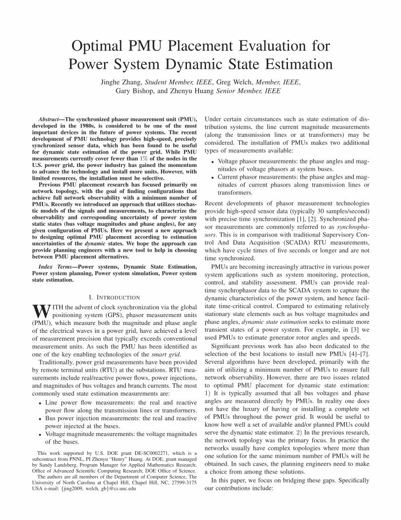
A. Estimation Uncertainty of a Fully PMU-installed System

We carried out our steady-state uncertainty analysis on asmall test system consisting of three machines in a loopednetwork of nine buses as shown in Fig. 1(a). The dynamicstate vector is x = {δ1, ω1, δ2, ω2, δ3, ω3}. To better illustratethe results, we represent the entire set of interest points x̂ ={δ1, δ2, δ3} ∈ [0, 2π]3 by a 3D grid. For each point x̂i, weobtain a 6 × 6 steady-state error covariance matrix P∞

i , andthen aggregate the information in P∞

i to the following valuefor visualization

f(x̂i) =

∑j=1,3,5

√P∞i[j,j]

+ wBΔt∑

j=2,4,6

√P∞i[j,j]

3, (45)

where we use Δt to convert speeds to changes in angle overthe inter-measurement period. Because√

P∞i[2k−1,2k−1]

+ wBΔt√P∞i[2k,2k]

·Δt (46)

represents the uncertainty in estimating the rotor angle ofgenerator k over time Δt, the value f(x̂i) is the averageuncertainty of the three generators over Δt at this particularpoint x̂i.

To begin with we consider an ideal scenario, where PMUsare installed on all the nine buses. Fig. 1(b) illustrates thef(x̂) values throughout the [0, 2π]3 space. One can clearly tella periodic pattern in the plot, because the Jacobian parametermatrices involve trigonometric functions of x̂. The darker areasreflect lower uncertainty, hence imply better expected estima-tion. This ideal case indicates the best estimation uncertaintylevel we can reach with a PMU placed on every bus.

B. Comparison Among Multiple Optimal Solutions

In this subsection, we used the same test system in Fig. 1(a)as an example of finding the optimal PMU placement solution.

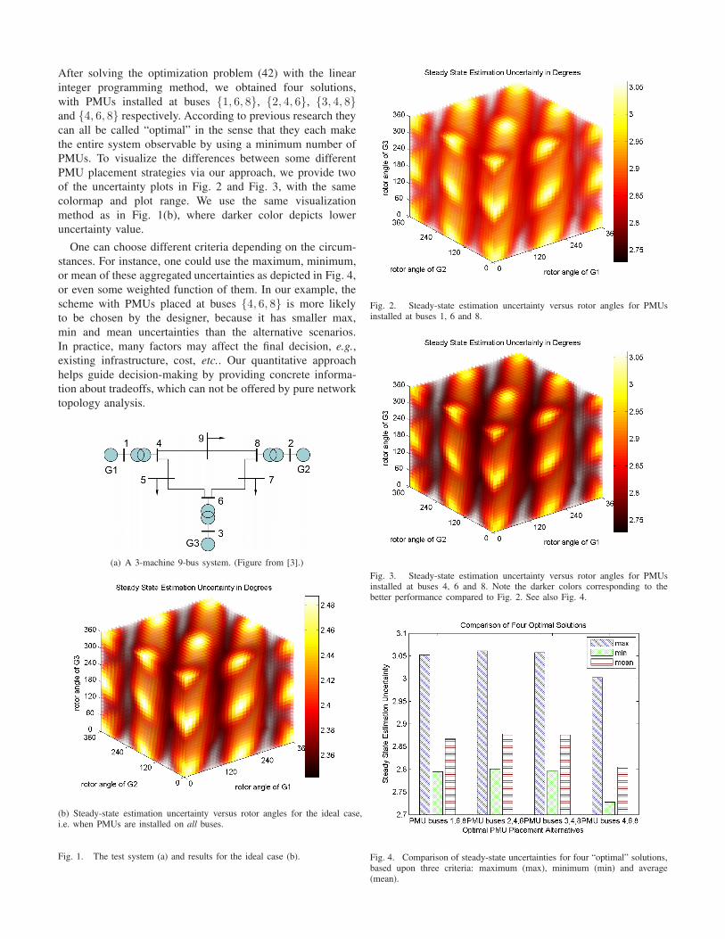
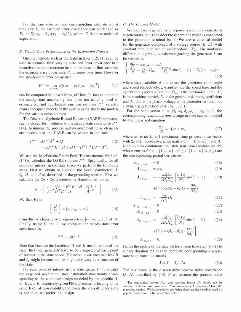
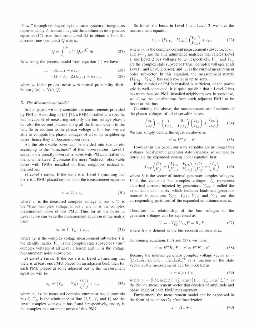
After solving the optimization problem (42) with the linearinteger programming method, we obtained four solutions,with PMUs installed at buses {1, 6, 8}, {2, 4, 6}, {3, 4, 8}and {4, 6, 8} respectively. According to previous research theycan all be called “optimal” in the sense that they each makethe entire system observable by using a minimum number ofPMUs. To visualize the differences between some differentPMU placement strategies via our approach, we provide twoof the uncertainty plots in Fig. 2 and Fig. 3, with the samecolormap and plot range. We use the same visualizationmethod as in Fig. 1(b), where darker color depicts loweruncertainty value.

One can choose different criteria depending on the circum-stances. For instance, one could use the maximum, minimum,or mean of these aggregated uncertainties as depicted in Fig. 4,or even some weighted function of them. In our example, thescheme with PMUs placed at buses {4, 6, 8} is more likelyto be chosen by the designer, because it has smaller max,min and mean uncertainties than the alternative scenarios.In practice, many factors may affect the final decision, e.g.,existing infrastructure, cost, etc.. Our quantitative approachhelps guide decision-making by providing concrete informa-tion about tradeoffs, which can not be offered by pure networktopology analysis.

(a) A 3-machine 9-bus system. (Figure from [3].)

(b) Steady-state estimation uncertainty versus rotor angles for the ideal case,i.e. when PMUs are installed on all buses.

Fig. 1. The test system (a) and results for the ideal case (b).

Fig. 2. Steady-state estimation uncertainty versus rotor angles for PMUsinstalled at buses 1, 6 and 8.

Fig. 3. Steady-state estimation uncertainty versus rotor angles for PMUsinstalled at buses 4, 6 and 8. Note the darker colors corresponding to thebetter performance compared to Fig. 2. See also Fig. 4.

Fig. 4. Comparison of steady-state uncertainties for four “optimal” solutions,based upon three criteria: maximum (max), minimum (min) and average(mean).

VI. CONCLUSIONS

We have presented a stochastic framework to quantify thesteady-state performance of any candidate PMU placementdesign, and reformulated the optimal PMU placement problemto tie it in with dynamic state estimation. This method can bereadily used without running the actual estimation procedure.We applied the method to a test system, and visualized theresults for several candidate PMU placements.

While we initially chose to work with PMU measurementsonly, we plan to extend the measurement set to includeconventional RTU measurements. We also plan to employour steady-state approach in a system-wide sensor placementoptimization framework.

VII. ACKNOWLEDGEMENTS

At the Pacific Northwest National Laboratory we acknowl-edge Ning Zhou, Pengwei Du, and Ruisheng Diao for helpfulbackground discussions. This work is supported by U.S. De-partment of Energy grant DE-SC0002271 “Advanced KalmanFilter for Real-Time Responsiveness in Complex Systems,”PIs Zhenyu Huang at PNNL and Greg Welch at UNC. AtDOE we acknowledge Sandy Landsberg, Program Manager forApplied Mathematics Research; Office of Advanced ScientificComputing Research; DOE Office of Science.

REFERENCES

[1] A. Phadke, J. Thorp, and M. Adamiak, “A new measurement techniquefor tracking voltage phasors, local system frequency, and rate of changeof frequency,” Power Apparatus and Systems, IEEE Transactions on,vol. PAS-102, no. 5, pp. 1025 –1038, may 1983.

[2] A. G. Phadke, J. S. Thorp, and K. J. Karimi, “State estimlatjon withphasor measurements,” Power Systems, IEEE Transactions on, vol. 1,no. 1, pp. 233 –238, feb. 1986.

[3] Z. Huang, K. Schneider, and J. Nieplocha, “Feasibility studies of apply-ing kalman filter techniques to power system dynamic state estimation,”in Power Engineering Conference, 2007. IPEC 2007. International, 3-62007, pp. 376 –382.

[4] T. Baldwin, L. Mili, J. Boisen, M.B., and R. Adapa, “Power systemobservability with minimal phasor measurement placement,” PowerSystems, IEEE Transactions on, vol. 8, no. 2, pp. 707 –715, may 1993.

[5] J. Chen and A. Abur, “Placement of pmus to enable bad data detection instate estimation,” Power Systems, IEEE Transactions on, vol. 21, no. 4,pp. 1608 –1615, nov. 2006.

[6] B. Gou, “Generalized integer linear programming formulation for op-timal pmu placement,” Power Systems, IEEE Transactions on, vol. 23,no. 3, pp. 1099 –1104, aug. 2008.

[7] B. Xu and A. Abur, “Observability analysis and measurement placementfor systems with pmus,” in Power Systems Conference and Exposition,2004. IEEE PES, 10-13 2004, pp. 943 – 946 vol.2.

[8] C. Madtharad, S. Premrudeepreechacharn, and N. R. Watson,“Power system state estimation using singular value decomposition,”Electric Power Systems Research, vol. 67, no. 2, pp. 99 – 107,2003. [Online]. Available: http://www.sciencedirect.com/science/article/B6V30-48JSMC9-1/2/39cddf1bf10c8ef84a9961dd54157556

[9] J. Zhang, G. Welch, and G. Bishop, “Observability and estimation un-certainty analysis for pmu placement alternatives,” (under submission),2010.

[10] B. D. Allen and G. Welch, “A general method for comparing theexpected performance of tracking and motion capture systems,” in VRST’05: Proceedings of the ACM symposium on Virtual reality software andtechnology. New York, NY, USA: ACM, 2005, pp. 201–210.

[11] B. D. Allen, “Hardware design optimization for human motion trackingsystems,” Ph.D. Dissertation, The University of North Carolina atChapel Hill, Department of Computer Science, Chapel Hill, NC, USA,November 2007.

[12] R. E. Kalman, “A new approach to linear filtering and predictionproblems,” Transaction of the ASME—Journal of Basic Engineering,vol. 82, no. Series D, pp. 35–45, 1960.

[13] G. Welch and G. Bishop, “An introduction to the kalman filter,”University of North Carolina at Chapel Hill, Department of ComputerScience, Tech. Rep. TR95-041, 1995.

[14] S. Grewal, Mohinder and P. Andrews, Angus, Kalman Filtering Theoryand Practice, ser. Information and System Sciences Series. UpperSaddle River, NJ USA: Prentice Hall, 1993.

Jinghe Zhang is a graduate student in computerscience at the University of North Carolina (UNC)at Chapel Hill. Her current research interests includeoptimal sensor placement for the power grid, andlarge scale estimation in general. Zhang has a B.S.from the University of Science and Technology ofChina (2006), and an M.S. from the University ofIdaho (2008), both in mathematics.

Greg Welch is a research associate professor ofcomputer science at the University of North Carolina(UNC) at Chapel Hill. His primary research areasinclude stochastic estimation, virtual and augmentedreality, human tracking systems, and 3D telepres-ence. Welch has a B.S.E.T. from Purdue University(1986), and a Ph.D. in computer science from UNC-Chapel Hill (1995). He is a member of the IEEEComputer Society and the ACM.

Gary Bishop is a professor of computer science atthe University of North Carolina (UNC) at ChapelHill. His current research interests include applica-tions of computer technology to address the needsof people with disabilities, and systems for man-machine interaction. Bishop has a B.S.E.E.T. fromSouthern Technical Institute (1976) and a Ph.D. incomputer science from UNC-Chapel Hill (1984).

Zhenyu Huang is a staff research engineer at thePacific Northwest National Laboratory, Richland,WA, and a licensed professional engineer in the stateof Washington. His research interests include powersystem stability and control, high-performance com-puting applications, and power system signal pro-cessing. Huang (M’01, SM’05) received his B. Eng.from Huazhong University of Science and Tech-nology (1994) and Ph.D. from Tsinghua University(1999).