optimal placement of convex polygons to maximize point containment

ELSEVIER Computational Geometry 11 (1998) 1-16

C o m p u t a t i o n a l

G e o m e t r y Theory and Applications

Optimal placement of convex polygons to maximize point containment

M a t t h e w D i c k e r s o n *, I, Dan ie l Schars te in 2

Department of Mathematics and Computer Science, Warner Hall Middlebury College, Middlebury, VT 05753, USA

Communicated by David Kirkpatrick; submitted 1 June 1996; accepted 23 February 1998

Abstract

Given a convex polygon P with m vertices and a set S of n points in the plane, we consider the problem of finding a placement of P (allowing both translation and rotation) that contains the maximum number of points in S. We present first an algorithm requiting O(nekm 2 log(mn)) time and O(n +m) space, where k is the maximum number of points contained. We then give a refinement that makes use of bucketing to improve the running time to O(nk2c2m 2 log(mk)), where c is the ratio of length to width of the polygon. This provides an improvement over the best previously known algorithm linear in n when k is large (®(n)) and a cubic when k is small. We also show that the algorithm can be extended to solve bichromatic and general weighted variants of the problem. The algorithm is self-contained and utilizes the geometric properties of the containing regions in the parameter space of transformations. © 1998 Elsevier Science B.V. All tights reserved.

Keywords: Maximizing placement; Rotation diagram

1. Introduction

A planar rigid motion p is an affine transformation of the plane that preserves distance (and therefore angles and area also). We say that a polygon P contains a set S of points if every point in S lies on the boundary of P, denoted a P, or in the interior of P. In this paper, we examine the following problem.

P rob l e m 1 (Optimal polygon placement). Given a convex polygon P and a planar point set S, find a rigid motion p that maximizes the number of points contained by p(P) . Report p and the subset of S contained by p(P) .

* Corresponding author. E-mail: [email protected]. 1 Supported by funds of the National Science Foundation CCR-9301714. 2 Supported by funds of the National Science Foundation IRI-9057928. E-mail: [email protected].

0925-7721/98/$19.00 © 1998 Elsevier Science B.V. All rights reserved. PII: S0925-7721(98)00015-7

2 M. Dickerson, D. Scharstein/Computational Geometry 11 (1998) 1-16

A similar optimization problem has been studied for fixed-radius circles [6]. Finding a placement of a circle to contain a maximum number of points has several applications, including placing a radio station of fixed transmission power so that the maximum population can receive the signal, and planning telescope observations to cover as many galaxies as possible [14]. There are also applications to clustering, line detection, and statistical analysis.

Here, we generalize the problem to the placement of convex polygons. This problem has previously been studied and solved for the restricted case of translation only [2,9]. We are not aware of previously published solutions for the general case of translation and rotation.

An extension of our algorithm to weighted point sets (see Section 4) has further applications, including placing labels on maps to avoid covering too much other information [15,20], or cutting a given piece out of a leather hide including as few flaws as possible [12]. Our algorithm has also been extended to solve a polygon annulus placement problem, with applications to geometric tolerancing, robot localization, and geometric pattern matching [1].

1.1. Background

Finding a transformation of a region such that it contains a given point set or subset is a problem that has received considerable attention in the past [2,4,7,9,11,13,16,18,19]. An interesting variant of the problem is to find an optimal placement of a given polygon that maximizes the number of points contained. Several authors have proposed algorithms for different versions of this problem, constraining either the shape of the polygon or the kind of allowed transformation.

Eppstein and Erickson [11], as a substep of their algorithm to find the minimum L~ diameter k-subset of a given set S, note that an algorithm of Overmars and Yap [17] can be modified to find the maximum depth of an arrangement of axis-aligned rectangles. This approach solves in O(n log n) time the problem of finding an optimal translation of a rectangle to cover the maximum sized subset of S. That is, it solves Problem 1 in O(n logn) time in the special case when the polygon is a rectangle and placement is restricted to translation only. Efrat et al. [9], as a substep in their algorithm for finding the smallest k-enclosing homothetic copy of an m-vertex polygon, claim an oracle solving the translation version for general m-vertex convex polygons. They suggest a line-sweep technique for their oracle, yielding an algorithm running in O(nklognlogm) time. Barequet et al. recently showed that the optimizing translation of a convex polygon can be found in O(nk log(mk)) time and O(m + n) space using anchored sweeps around points in S [2].

When we allow general rigid motion (translation and rotation) as in Problem 1, less is known. Chazelle [5] gave a definition of a stable placement of two polygons P and Q with P containing Q and general rigid motion allowed.

Definition 1 (Chazelle). Polygons P and Q are in a stable placement with P containing Q if and only if one of the following conditions holds: (1) at least 3 vertices in Q lie on 8P, or (2) at least 2 vertices in Q lie on 8 P and at least one vertex of Q lies on a vertex of P.

It was shown in [5] that if some polygon P contains a polygon Q, then there exists a stable placement of P and Q with P still containing Q. Furthermore, all stable placements of an m-vertex polygon P on three points (of which there may be ®(m2)) can be computed in O(m 2) time. For Problem 1, a brute-

M. Dickerson, D. Scharstein / Computational Geometry 11 (1998) 1-16 3

force approach based on this result could, for each triple of points in S, compute all stable placements of P, and for each of these n3m 2 placements count in O(n logm) time the number of points contained. This leads to an O(n4m 2 log m) time algorithm.

Eppstein has pointed out in a personal communication [10] that the problem can also be solved in O(n2kam 2 logm) time using techniques of [11]. He noted that the set covered by the optimal polygon placement is a subset of the O(k) nearest points in vertical distance to some segment pq, where p and q are the maximum and minimum points (with respect to x-coordinate) of the optimal set. In other words, let p and q be the leftmost and rightmost points covered by the optimal placement. Then the other k - 2 points not only have to project vertically onto segment pq but also have to be among the ck points nearest to segment pq in vertical distance. This reduces the problem to searching O(n 2) subsets (those generated by accepting every pair (p, q) as possible endpoints) of O(k) points each. For each subset, apply the technique described in the previous paragraph to ck points instead of n points. This yields an O(n2k4m210gm) time solution. Though k may be as large as n, making this an ~'~(n 6) algorithm in the worst case, it does present an "output-sensitive" approach and shows that the dependence on n can be reduced to quadratic. In the case where k is small, this method provides the best previously known algorithm.

1.2. Outline of our approach

In this paper we provide a new algorithm for Problem 1 that requires only O(n2km 2 log(mn)) time and O(m + n) space. The basic idea of the algorithm is as follows.

For each point qi 6 S, we identify all transformations p of the polygon P that keep qi on its boundary. We capture these transformations geometrically in the rotation diagram, a compact geometric characterization of a two-dimensional subset of the parameter space. Each other point qj yields a containing region in the rotation diagram which can be decomposed into O(m 2) subregions of constant complexity, and can be computed efficiently by considering the intersections of two rotating copies of P. We search the arrangement of all containing regions using a line sweep to find the translation-stable placement yielding maximum point containment.

We also provide a variant of our algorithm in which we reduce our search space by using a bucketing approach to eliminate points that are too far from qi to be contained by a placement of P with qi on the boundary. If we consider the length to width ratio of the polygon as a constant, then this bucketing approach requires only O(nkZm 2 log(ink)) time, which is linearly faster in n than the approach without bucketing if the number k of points covered is small.

The rest of the paper is organized as follows. In Section 2 we present some definitions and geometric lemmas upon which our algorithm is based. In Section 3 we present our algorithm along with an analysis and proof of correctness. In Section 4, we generalize our algorithm to solve the bichromatic variant of our problem, as well as a general weighted variant. Section 5 provides our summarizing remarks and some open related problems.

2. Geometric and algorithmic preliminaries

We now present some geometric results necessary for our algorithm. We begin with some definitions and notation that will be used throughout the paper.

4 M. Dickerson, D. Scharstein/Computational Geometry 11 (1998) 1-16

We use qi to represent the ith point in our input set S. We assume that the polygon P is represented as a list of its vertices Vl . . . . . Vm given in clockwise order, with vl located at the origin. We use the standard notation 0 P to represent the boundary of the polygon P, i.e., the union of the edges and vertices of P.

2.1. Stable placements

Stable placements play a fundamental role in our algorithm, allowing us to consider only a finite subset of the infinite number of all possible placements. Extending Chazelle's idea of stable placement of two polygons, Barequet et al. [2] gave the following definition for the translation stable placement of a polygon with respect to a point set.

Definition 2. Let r ( P ) be a translation of a polygon P. We say that r ( P ) is in translation stable placement with respect to a set of points S if at least 2 points in S are on 0 P.

In our algorithm, we use a simplified version of a result of Chazelle's [5].

Lemma 1. Let S be a planar point set and P a convex polygon. If there is a rigid motion p such that p (P) contains k >>, 2points in S, then there exists a rigid motion p* such that p*(P) contains at least k points in S with at least one point in S on the boundary Op* ( P).

We also use the following lemma (which was stated and proven in a slightly different form in [2]) relating intersections of polygons and translation stable placements.

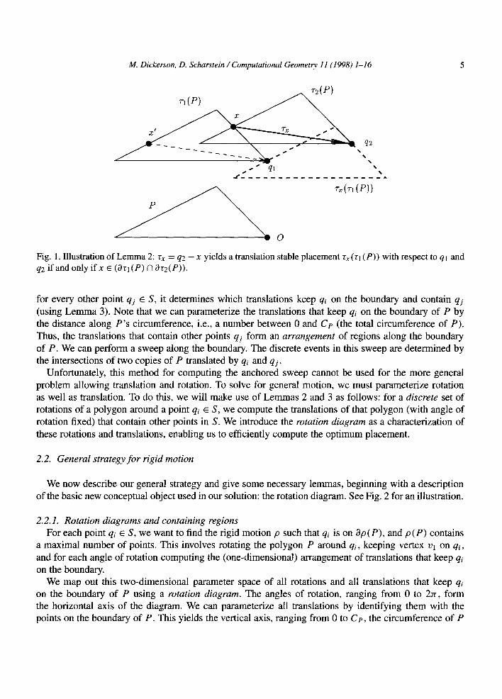
Lemma 2 (Barequet, Dickerson and Pau). Let P be a convex polygon, ql, q2 points, and ~1 and r2 the translations mapping the origin to points ql and q2 respectively. For any point x on Orl( P), define rx = q2 - x as the translation that maps x to q2. Then x is a point of intersection between Orl(P) and Or2(P) if and only if ql is on 0rx(rl (P)). (Note that q2 must be on OZx(rl (P)) by the definition Of rx.)

The proof of the lemma follows from simple vector arithmetic (see Fig. 1). Let x' = x + ql - - q2 be the point on r I (P) corresponding to x on rE(P). The vector rx maps x' to ql and x to q2. Since x' and x are both on r l (P) , ql and q2 are both on Zx(rl(P)).

What this lemma tells us is that the points of intersection between two translated copies of a convex polygon P determine all translations of P that are in translation stable placement with respect to these points. Specifically, rx (rl (P)) is in translation stable placement with ql and q2 on Or: x (/~1 ( P ) ) if and only if x is a point of intersection between 0z~ (P) and Or2(P).

The lemma easily generalizes to the following lemma on containment of two points ql and q2-

Lemma 3. Let P be a convex polygon, ql, q2 points, and r 1 and r2 the translations mapping the origin to points ql and q2, respectively. For any point x, define Zx = q2 - x as the translation that maps x to q2. Then x E ( / : I ( P ) f ' ) / : 2 (P ) ) if and only if rx(zl(P)) contains both ql and q2.

For a proof, consider again x' --- x + ql - q2- If x is in rz(P) then x' is in r l (P) , rx maps x to q2 and x' to ql. But x' and x are both in Zl (P), so ql and q2 are both in rx (rl (P)) .

To solve the simpler problem of maximal point containment for translation only, the algorithm of [2] performs an "anchored sweep" of the polygon P around each point in S. That is, for a given qi ~ S and


n(P) / / i ~ (P)

X /

q2

s

T~(7"1 (P))

O

%

Fig. 1. Illustration of Lemma 2: rx = q2 - - x yields a translation stable placement rx ( r l (P)) with respect to ql and q2 if and only ifx ~ (0rl(P) A 0r2(P)).

for every other point qj E S, it determines which translations keep qi on the boundary and contain qj (using Lemma 3). Note that we can parameterize the translations that keep qi on the boundary of P by the distance along P ' s circumference, i.e., a number between 0 and Cp (the total circumference of P). Thus, the translations that contain other points qj form an arrangement of regions along the boundary of P. We can perform a sweep along the boundary. The discrete events in this sweep are determined by the intersections of two copies of P translated by qi and qj.

Unfortunately, this method for computing the anchored sweep cannot be used for the more general problem allowing translation and rotation. To solve for general motion, we must parameterize rotation as well as translation. To do this, we will make use of Lemmas 2 and 3 as follows: for a discrete set of rotations of a polygon around a point qi E S, we compute the translations of that polygon (with angle of rotation fixed) that contain other points in S. We introduce the rotation diagram as a characterization of these rotations and translations, enabling us to efficiently compute the optimum placement.

2.2. General strategy for rigid motion

We now describe our general strategy and give some necessary lemmas, beginning with a description of the basic new conceptual object used in our solution: the rotation diagram. See Fig. 2 for an illustration.

2.2.1. Rotation diagrams and containing regions For each point qi E S, w e want to find the rigid motion p such that qi is on Op(P), and p(P) contains

a maximal number of points. This involves rotating the polygon P around qi, keeping vertex v~ on qi, and for each angle of rotation computing the (one-dimensional) arrangement of translations that keep qi on the boundary.

We map out this two-dimensional parameter space of all rotations and all translations that keep qi on the boundary of P using a rotation diagram. The angles of rotation, ranging from 0 to 2Jr, form the horizontal axis of the diagram. We can parameterize all translations by identifying them with the points on the boundary of P. This yields the vertical axis, ranging from 0 to Cp, the circumference of P

M. Dickerson, D. Scharstein / Computational Geometry 11 (1998) 1-16

01 02 03 07 05 06 Vl

V2

'03

0 90 180 270 360 "01

Fig. 2. An example of a containing region Aq2 in the rotation diagram Rp,ql for a triangle P. The critical angles are marked 01 through 06.

(normalized to 1 in Fig. 2). We call the resulting two-dimensional space the rotation diagram Rp,qi. Note that both axes of Rp,q i "wrap around", since 0 and 2zr, and also 0 and Cp are identified. (In terms of topology, the rotation diagram forms the surface of a torus.) Each point (0, t) in Rp.q i corresponds to the placement of P rotated by 0 and translated such that the point at position t along P ' s circumference is identified with qi.

Given other points in S, we can then map out their containing regions in the rotation diagram, allowing us to geometrically capture the optimal placement of P. We illustrate this idea in the following section for only one extra point, and give several lemmas necessary for both our proof of correctness and run-time analysis.

2.2.2. Pairs of rotating polygons Consider placing two copies P1 and P2 of a polygon P on points ql, q2 E S. Specifically, we place

vertex Vl of P on each of the two points. We now rotate the two polygons in tandem and examine what happens. By Lemma 2, at any given angle of rotation the intersections between the two polygons determine the translations of P which would place both ql and q2 on the boundary of P. As we rotate the pair of polygons, these translations trace out curves in the rotation diagram Rp,q~ for P and ql. By Lemma 3, these curves are the boundary of a (not necessarily connected) containing region in Rp,q~ corresponding to all placements of P that contain q2 (and have ql on the boundary). Let us call this region Aq2. We will now study the properties of Aq2.

At each angle 0 we can imagine a vertical line in Rp,ql representing the "unfolded" boundary of the polygon P rotated by 0. Note that such a line can intersect at most two of the bounding curves, since two copies of the same convex polygon at the same orientation can intersect in at most two distinct points (or, in the degenerate case, along a consecutive part of the boundary). In between these two intersection points, the line intersects the containing region Aq2. The intersection corresponds to the part of the boundary of Pl that is covered by P2. We now decompose Aq2 into smaller regions bounded on the left and right by certain critical angles: namely those angles at which a vertex of P1 sweeps through 8 P2 or a vertex of P2 sweeps through 0 P1 (see Fig. 3). Each decomposed region has four sides, and it is clear by definition that the left and right sides are vertical lines at the critical angles. In the case that


. . - . . . . . . .

, ..

.-' ~ . / ",\ ~ " ." \ "~. " ~ Z . ' , .

i ', ..

• ."

" ' . . . '

" . . . . . . . . . . . -

Fig. 3. The underlying geometry for the rotation diagram in Fig. 2. The critical angles correspond to intersections of circles with edges.

at a critical angle the polygons start (or stop) being in contact with each other, a vertical bounding line might degenerate to a point. Fig. 2 shows an example of a containing region in a rotation diagram for a triangle. The containing region Aq2 is traced out by vertical lines; the critical angles are shown by dotted lines. Remember that the diagram wraps around.

The obvious next question to ask is: what kind of curves form the top and bottom boundaries of the containing region? Lemma 4 answers this question, and Lemmas 5 and 6 deal with the size and number of the decomposed regions.

Lemma 4. The upper and lower curves bounding the decomposed regions of Aq2 are sine curves of the form cl + c2 sin(0 + c3).

Proof. The key observation for this proof is that rotating two polygons in tandem is equivalent to keeping one of the polygons fixed, and translating the other polygon on a circle around it. No rotation needs to take place, since the relative orientation of the two polygons to each other remains constant. Specifically, if we keep PI in place, every vertex of P2 describes a circle around the corresponding vertex of Pl (see Fig. 3). All circles have the same radius r, which is equal to the distance between the points ql and q2. Between two critical angles, a bounding curve of Aq2 is created by some edge ee of P2 intersecting an edge el of P1- The y-coordinate in the rotation diagram is the position of the intersection point on the circumference of P1, i.e., the position of the intersection point on el plus the length l of all previous edges of PI. To show that the position of the point of intersection on an edge with another edge sweeping out a circle is a multiple of a sine function, let us reorient the coordinate system by a translation that places the center of rotation at the origin, and by an angle of rotation F such that e2 is now vertical. Now, e2 intersects the x-axis at r sinot, where ot = 0 - y. Let ~b be the orientation of el in our new coordinate

8 M. Dickers®n, D. Scharstein/Computational Geometry 11 (1998) 1-16

el f . . . o

x0 I . . . . . . . r - ~

Fig. 4. Illustration of Lemma 4: edge ex translating on a circle intersects edge el at position x0 + (r/cos ~b) sin or.

system, and let x0 be the length of the part of el that lies to the left of the y-axis (see Fig. 4). Then, the intersection point on the circumference of P1 is at l + x0 + (r/cos ~b) sin(0 - y) , or Cl + c2 sin(0 + c3). []

Lemma 5. Each decomposed region is at most Jr wide.

Proof. A decomposed region is bounded by two critical angles, which are created by vertices sweeping through edges of the other polygon. The maximum width of the regions is bounded by the maximal part of a circle---centered on a vertex--that lies inside the polygon, that is, by the biggest angle of the polygon. Since the polygon is convex, the biggest possible angle is re. []

Lemma 6. Aq2 is decomposed into at most ®(m 2) regions.

Proof. Polygon P has m vertices and edges. Since the path of each vertex is traced by a circle, a vertex can sweep through each edge of the other polygon at most twice yielding at most 2m critical angles per vertex, or O(m 2) total critical angles. []

Note that the bound given in Lemma 6 is tight, i.e., there are cases yielding ®(m 2) decomposed regions. Fig. 5 illustrates an example. We construct a polygon by placing m/ 2 vertices such that they form a quarter of a regular 4(m/2 - 1)-gon, intersecting the unit circle m times (the intersections are marked with crosses). Let e be the maximum variation of the radius of the circle still yielding m intersections. Place the other m/2 vertices such that they form a rounded comer less than e away from the origin. Now, for two points ql, q2 of distance 1, the rotation diagram has ®(m 2) critical angles as the m / 2 closely spaced vertices of each copy of the polygon intersect edges of the other copy of the polygon m times as 0 ranges from 0 to 2zr.

2.2.3. Generalization to multiple points For a given point qi, we can compute the containing regions Aqj in Rp,qi for all other points qj E S

and j 5~ i. For points qj and qk, the regions Aqj and Aqk may intersect, indicating a placement of P


. " E I .--4--- . ' " I " ,

T - - ; - -

" . I o "

I I

Fig, 5. A polygon yielding m 2 critical angles (m = 8 in the figure). Half of the vertices form a quarter of a regular polygon that intersects the unit circle m times, the other half are closely spaced next to the origin.

\ \

C 0 90 180 270 360

Fig. 6. An arrangement of four containing regions. The deepest point in the arrangement is marked with a white dot. The corresponding transformation of the polygon (yielding containment of all four points) is drawn on the left. The transformation corresponding to the origin of the rotation diagram is shown dashed.

containing qi, qj and qk- The deepest point in the arrangement of all containing regions gives us the rotation and translation keeping qi on the boundary and containing the maximum number of other points in S. We compute these arrangements of containing regions for all rotation diagrams Re,qi and compute the deepest arrangement in all n diagrams. See Fig. 6 for an example of an arrangement of four containing regions.

10 M. Dickerson, D. Scharstein / Computational Geometry 11 (1998) 1-16

2.3. Other applications of the rotation diagram

Besides the problem considered in this paper, rotation diagrams also have applications in robot motion planning: Note that the rotation diagram Rp,q represents the configuration space of a convex polygonal robot P that must stay in contact with a point q (say, a power source). A path in Rp,q that does not cross any boundaries of containing regions corresponds to a collision-free motion of P avoiding (or containing) a given set of points while keeping q on the boundary of P. The tools to compute and search arrangements of containing regions in rotation diagrams developed in this paper can also be used to compute such collision-free paths efficiently.

3. The algorithm

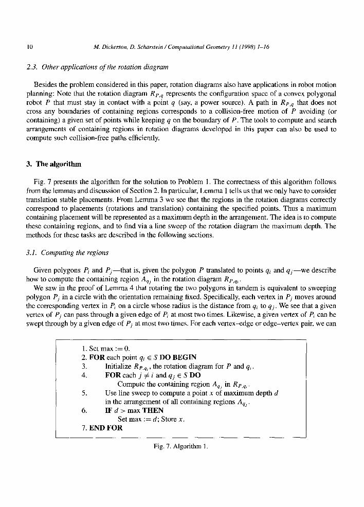
Fig. 7 presents the algorithm for the solution to Problem 1. The correctness of this algorithm follows from the lemmas and discussion of Section 2. In particular, Lemma 1 tells us that we only have to consider translation stable placements. From Lemma 3 we see that the regions in the rotation diagrams correctly correspond to placements (rotations and translation) containing the specified points. Thus a maximum containing placement will be represented as a maximum depth in the arrangement. The idea is to compute these containing regions, and to find via a line sweep of the rotation diagram the maximum depth. The methods for these tasks are described in the following sections.

3.1. Computing the regions

Given polygons Pi and Pj- - that is, given the polygon P translated to points qi and q j - - w e describe how to compute the containing region Aqj in the rotation diagram Rp,qi.

We saw in the proof of Lemma 4 that rotating the two polygons in tandem is equivalent to sweeping polygon Pj in a circle with the orientation remaining fixed. Specifically, each vertex in Pj moves around the corresponding vertex in Pi on a circle whose radius is the distance from qi tO qj. We see that a given vertex of Pj can pass through a given edge of Pi at most two times. Likewise, a given vertex of P/can be swept through by a given edge of Pj at most two times. For each vertex-edge or edge-vertex pair, we can

1. Set max := 0. 2. FOR each point qi E S DO BEGIN 3. Initialize Rp,qg, the rotation diagram for P and qi. 4. FOR each j ~ i and qj ~ S DO

Compute the containing region Aqj in Rp,q i . 5. Use line sweep to compute a point x of maximum depth d

in the arrangement of all containing regions Aqj. 6. IF d > max THEN

Set max := d; Store x. 7. END FOR

Fig. 7. Algorithm 1.


explicitly compute the angles of rotation causing an intersection in constant time by intersecting a circle with a segment. We have a total of m 2 work to compute these angles. We sort these in O(m 2 logm) time, and use them to compute at most m 2 decomposed regions of Aqj.

3.2. Complexity of the arrangements via line sweep

Given the rotation diagram Rp,qi for a point qi, we now show how the depth of the arrangement of all containing regions Aqj, j ~ i, in Rp,q i can be found. We sweep a vertical line through all angles of rotation 0. The events in the line sweep consist of the discrete set of angles marking the left and fight boundaries of the decomposed regions, and the intersections of sine curves forming the top and bottom boundaries of the decomposed regions with other boundaries. We need a data structure to keep track of these boundaries so that we can quickly search, insert and delete boundaries, as well as swap their order in the case of an intersection event. An efficient data structure for this is a segment tree, which we modify for sine curves. The segment tree was introduced by Bentley [3] and is also described in [18, pp. 13-15]. A version that handles degeneracy without special cases is described in [8, pp. 22-29]. The segment tree is a binary search tree that keeps track of the vertical ordering of a set of line segments (in our case sine curves) at a particular x-coordinate. At the left (respectively right) boundaries of a region we add (delete) sine curves to the tree, and at each intersection event two such sine curve boundaries swap locations in the tree. In all of these cases, we need to compare all newly created neighbors in the tree to check for new intersection events. If n is the number of segments in the tree, then all of the segment tree operations and thus all of our events require O(logn) time.

To analyze the efficiency of our line sweep, we thus need to count the number of critical events. Note first that in rotation diagram Rp,qi, there are n - 1 containing regions Aqj, each decomposed into at most

O(m 2) subregions. At any given angle, there are at most 2n - 2 sine curves to be stored in the segment tree. This data structure therefore requires O(n) space and O(log n) time per operation. How many queue events are there? We have just seen that there are at m o s t O ( n m 2) critical angles marking the left and fight sides of regions. So we need now count only intersection events.

3.2.1. A bound on the number of intersections Remember that in our rotation diagram Rp,qi, the region Aqj for a point qj corresponds to placements

containing qj and with qi on the boundary. So the upper and lower boundaries of the region Aqj correspond to placements of P with both qi and qj on the boundary. Finally, an intersection between the regions Aqj and Aqk corresponds to a stable placement with qi, qj and q~ all on the boundary. To bound the number of such intersection events in our line sweep, we therefore need only to bound the number of stable placements with qi and two other points on the boundary of P.

Theorem 1. Let P be a convex polygon and S a planar point set with qi E S. I f k is the maximum number of points that can be covered by a placement of P in contact with qi, then there are at most O(nkm 2) stable placements of P with qi and two other points in S on the boundary of P.

Proof. We will use an amortization approach to limit the number of possible stable placements. We charge each stable placement with qi, qj and qk on the boundary to whichever of qj and qk is the farthest from qi. For this we need the following lemma.


Lemma 7. Given points qi and qj separated by a distance r and a circle of radius r around qi, the fraction of the area of this circle that can be swept out by an (arbitrarily long) rectangle of width d containing both qi and qj is bounded by 5dr, and this swept area can be tiled by at most 6 overlapping copies of the rectangle.

The proof of Lemma 7 is given in Appendix A. We use the lemma as follows. In order for there to be a stable placement of P on qi and q j, there is also (by definition) a placement of P containing qi and qj. Assume this is the case. Now let R be the smallest rectangle containing polygon P. There must also be a placement of R containing qi and qj. Our amortization approach only charges to qj those stable placements where the third point (say q~) is at least as close to qi than qj. These points must be in the circle centered at qi whose radius is the distance from qi to qj. Lemma 7 bounds the area in which the third point qk can fall and still be covered by R, and says that 6 overlapping copies of R suffice to contain all the points in this region. For a given 3 points, there are O(m 2) placements. Let K be the number of points in this area. Thus Km 2 is the maximum number of placements that can possibly be charged to qi. Then by Lemma 7 there is a placement of R containing at least K/6 points. Or, conversely, assume that R was our polygon and let k be the maximum number of points contained in the optimal placement of R, then at most 6km 2 stable placements (intersection events) get charged to qj. However, it was shown in [2, Lemma 7] that a constant number of overlapping copies of P suffice to tile R, thus our bound still holds and there are O(km 2) stable placements (intersection events) that get charged to qj.

By our amortized analysis, there are n - 1 other points, each of which gets charged O(km 2) times for a total of O(nkm 2) stable placements in contact with qi. []

Corollary 1. The number of critical intersection events in the line sweep of a rotation diagram for a particular point in Algorithm 1 is O(nkm2).

3.2.2. Final analysis of Algorithm 1 So we see that for each of n rotation diagrams Rp,q i, the number of intersections between pairs of

containing regions is bounded by O(nkm2), where k is the maximal depth of all arrangements. For each of n diagrams we also have at most O(nm 2) critical angles marking left and right boundaries of subregions. Algorithm 1 therefore requires O(n2km 2 log(mn)) time and O(n + m) space. This analysis is independent of the shape of the polygon. The algorithm is asymptotically faster than those based on the results of [5] and [11] by factors of n2/k and k 3, respectively.

3.3. Bucketing

We now discuss a variant of Algorithm 1 that makes use of bucketing to give a tighter output sensitive time bound. Let D be the diameter of the polygon P. If C is a chord of P of length D, let W be the width of P perpendicular to C. Our bucketing strategy is to bucket space into squares of size D x D, and to place each point in its correct bucket. We use the following straightforward lemma for the analysis.

Lemma 8. Any bucket can be tiled by a fixed number c of copies of P, with c dependent only on the ratio D~ W. Furthermore, if any bucket contains K points, then there is a placement of P containing f2 ( K / c) points.

M. Dickerson, D. Scharstein / Computational Geometry 11 (1998) l-16 13

The idea of the proof is to construct a rectangle R' inscribed inside P and aligned with C, with sides having the same proportions as D and W. It is easy to see that the bucket can be tiled with ®(C/W) copies of R', and thus also of P.

A polygon containing a point qi in bucket b can contain only points in b and the 8 buckets neighbor- ing b. We call this group of 9 buckets Bi. We modify our algorithm as follows. First, we add a preprocessing phase.

0. Preprocessing. Preprocess points into buckets of size D x D. For all points qi E S, w e define Bi a s

the set of buckets that could intersect a placement of polygon P containing point qi.

We then replace step 4 with the following.

4. FOR each j ~ i and qj ~ Bi DO

Thus, in our construction of the rotation diagram Rp,qi for polygon P and point qi we consider only points in Bi.

3.4. Final analysis of the bucketing approach

The analysis of the bucketing approach remains almost identical: we replace each factor of n (except the outermost FOR loop of step 2) with a k. If we consider the length to width ratio of the polygon as a constant, this gives a running time of O(nkZm 2 log(mk)).

For "skinny" polygons with a large ratio c = D~ W, the bucketing approach may be inefficient: by Lemma 8, the number k of points covered is proportional to K/c where K is the number of points in the densest bucket. Thus, the exact running time is given by O(nKZm 2 log(mk)) = O(nk2cZm 2 log(mk)).

Theorem 2. Algorithm 1 requires O(n2km 2 log(mn)) time and O(n + m) space when no bucketing is used, and O(nk2m 2 log(mk)) time when bucketing is used.

4. Bichromatic and weighted variants

The algorithm presented here can easily be extended to a more general version of the problem. Consider a set S where each point qi is given a weight W(qi). Instead of maximizing the number of points covered, we want to maximize the total weights of all points contained. If all weights are greater than or equal to zero, then Lemma 1 still applies where k becomes the total weight of the contained points rather than the number of contained points. The only modification to the algorithm is that we keep track of placements of greatest weight instead of greatest number of points.

However, if W(qi) < 0 for some points in the set, then it is possible that there is no stable placement that maximizes the total weight of the points covered. (It is not difficult to give an example where the only stable placement covering the same points as that covered by the maximal placement also covers an additional negatively weighted point.) In particular, consider the bichromatic version where the set S is divided into two subsets Sr and Sb and the goal is to find a placement that maximizes the number of points contained from Sr and minimizes the number contained from Sb. This can be modeled as the weighted variant where all points in Sr have weight 1 and all points in So have weight -1 . Another


bichromatic problem, to maximize points covered in Sr while covering no point in Sb, can be solved by assigning weight 1 to the points in Sr and the weight - Ia r l to the points in Sb.

The solution to the problem is not difficult. For each placement p with a negatively weighted point qi on the boundary, we look for a "nearby" placement p~ that contains the same points but does not contain qi. The same idea can be applied in the degenerate case where multiple points lie on the boundary, though if there is more than one negatively weighted point on the boundary then the e translation will not necessarily exist. Thus with minor modifications, the algorithm can be used to solve both the bichromatic and the general weighted variant of the problem with the same running time.

5. Summary

We have provided the asymptotically fastest known solution to the problem of computing a placement (translation and rotation) of a given convex polygon P containing the maximum number of points of a given point set S. We have shown that the algorithm requires output-sensitive O(n2km 2 log(mn)) time and O(n + m) space, where n is the number of points in S, m is the number of vertices of P, and k is the maximum number of points contained (k ~< n). Using bucketing, we achieve a time bound of O(nk2c2m 2 log(mk)), where c is the width to length ratio of P. This bucketing variant is more "output sensitive" in that it is linearly faster in n when k is small (a constant), but it depends on the shape of the polygon P.

The algorithm we presented is conceptually simple and self-contained. It uses a line sweep of an arrangement of containing regions in a rotation diagram. The rotation diagram can also be used to solve motion planning problems in which a convex polygonal robot must stay in contact with a certain point while avoiding or containing other points. The algorithm generalizes at no cost in running time not only to solve the bichromatic variant of the problem, but the more general weighted point set problem. It is asymptotically faster than the best previously known approaches by at least a linear factor, and as much a s n 3 depending on k, the number of points covered.

A Java applet providing an interactive demonstration of the rotation diagram can be accessed at http : //www .middlebury. edu/-schar/rotate/.

5.1. Extensions and open problems

There are obvious generalizations of Problem 1.

Problem 2. Given a simple polygon P and a planar point set S, find a rigid motion (or even just a translation) p that maximizes the number of points contained by p(P).

Our algorithm can still be applied, but with a significant increase in complexity [1].

Problem 3. Given a convex polyhedron P and a point set S in R 3, find a rigid motion p that maximizes the number of points contained by p (P) over all possible rigid motions.


Acknowledgements

This paper benefited from discussions with Amy Briggs and the comments of the reviewers.

anonymous

Appendix A. Proof of Lemma 7

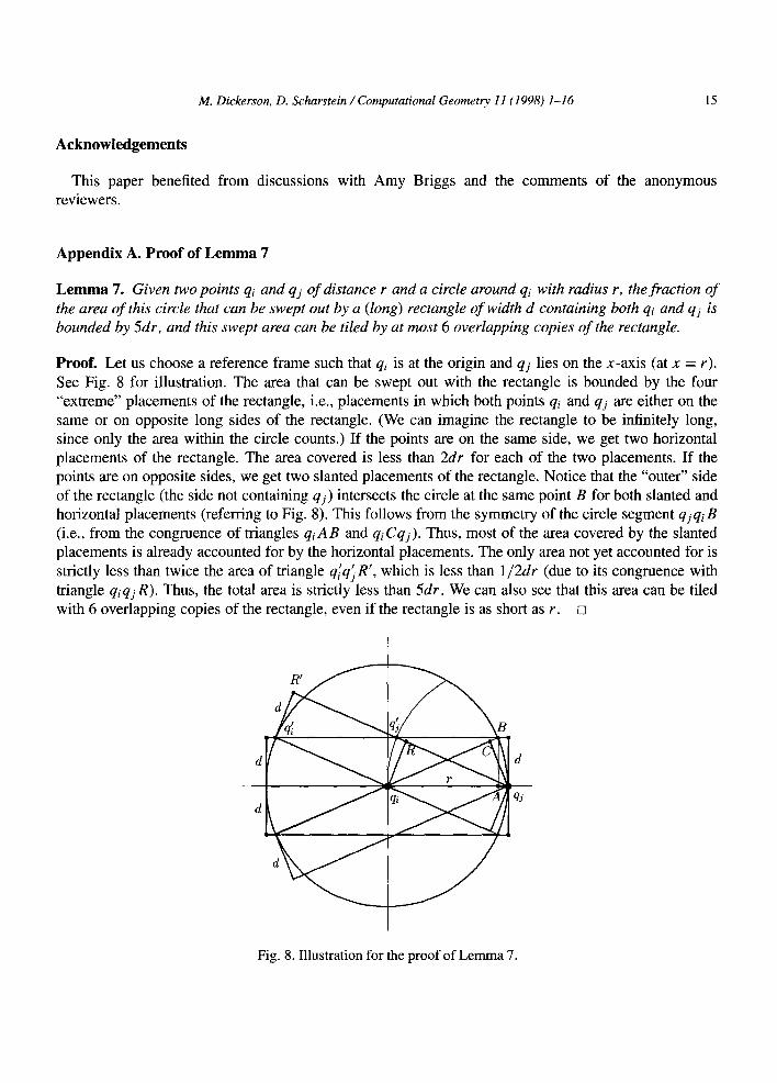
Lemma 7. Given two points qi and qj of distance r and a circle around qi with radius r, the fraction of the area of this circle that can be swept out by a (long) rectangle of width d containing both qi and qj is bounded by 5dr, and this swept area can be tiled by at most 6 overlapping copies of the rectangle.

Proof. Let us choose a reference frame such that qi is at the origin and qj lies on the x-axis (at x = r). See Fig. 8 for illustration. The area that can be swept out with the rectangle is bounded by the four "extreme" placements of the rectangle, i.e., placements in which both points qi and qj are either on the same or on opposite long sides of the rectangle. (We can imagine the rectangle to be infinitely long, since only the area within the circle counts.) If the points are on the same side, we get two horizontal placements of the rectangle. The area covered is less than 2dr for each of the two placements. If the points are on opposite sides, we get two slanted placements of the rectangle. Notice that the "outer" side of the rectangle (the side not containing q j) intersects the circle at the same point B for both slanted and horizontal placements (referring to Fig. 8). This follows from the symmetry of the circle segment qjqi B (i.e., from the congruence of triangles qiAB and qiCqj). Thus, most of the area covered by the slanted placements is already accounted for by the horizontal placements. The only area not yet accounted for is strictly less than twice the area of triangle q~q~ R', which is less than 1 ~2dr (due to its congruence with triangle qiqjR). Thus, the total area is strictly less than 5dr. We can also see that this area can be tiled with 6 overlapping copies of the rectangle, even if the rectangle is as short as r. []

Fig. 8. Illustration for the proof of Lemma 7.


References

[1] G. Barequet, A. Briggs, M. Dickerson, M. Goodrich, Offset-polygon annulus placement problems, in: Proc. 5th Annual Workshop on Algorithms and Data Structures, Lecture Notes in Computer Science, Vol. 1272, Springer, New York, 1997, pp. 378-391.

[2] G. Barequet, M. Dickerson, P. Pau, Translating a convex polygon to contain a maximum number of points, in: Proc. 7th Canadian Conference on Computational Geometry, 1995, pp. 61-66. Also: Computational Geometry: Theory and Applications 8 (1997) 167-179.

[3] J. Bentley, Algorithms for Klee's rectangle problems, Carnegie Mellon University, Unpublished notes, 1977. [4] S. Chandran, D. Mount, A parallel algorithm for enclosed and enclosing triangles, Computational Geometry:

Theory and Applications 2 (2) (1992) 191-214. [5] B. Chazelle, The polygon placement problem, in: E Preparata (Ed.), Advances in Computing Research, Vol. 1

(JAI Press, 1983) pp. 1-34. [6] B. Chazelle, D.T. Lee, On a circle placement problem, Computing 36 (1986) 1-16. [7] A. Datta, H.E Lenhof, C. Schwarz, M. Smid, Static and dynamic algorithms for k-point clustering problems,

in: Proc. 3rd Workshop on Algorithms and Data Structures, Lecture Notes in Computer Science, Vol. 709, Springer, New York, 1993, pp. 265-276.

[8] M. de Berg, M. van Kreveld, M. Overmars, O. Schwarzkopf, Computational Geometry: Algorithms and Applications, Springer, Berlin, 1997.

[9] A. Efrat, M. Sharir, A. Ziv, Computing the smallest k-enclosing circle and related problems, Computational Geometry: Theory and Applications 4 (1994) 119-136.

[10] D. Eppstein, 1995, Personal communication. [11] D. Eppstein, J. Erickson, Iterated nearest neighbors and finding minimal polytopes, Discrete Comput. Geom.

11 (1994) 321-350. [12] J. Heistermann, T. Lengauer, The nesting problem in the leather manufacturing industry, Ann. Oper. Res. 57

(1995) 147-173. [13] V. Klee, M.L. Laskowski, Finding the smallest triangles containing a given convex polygon, J. Algorithms 6

(1985) 359-375. [14] R. Lupton, E Miller Maley, N. Young, Data collection for the Sloan Digital Sky Survey - A network-flow

heuristic, in: Proc. 7th ACM-SIAM Symposium on Discrete Algorithms, 1996, pp. 296-303. [15] A. Mirzain, B. Zhu, Labeling a rectilinear map, in: Proc. 5th MSI Workshop on Computational Geometry,

1995. [16] J. O'Rourke, A. Aggarwal, S. Maddila, M. Baldwin, An optimal algorithm for finding minimal enclosing

triangles, J. Algorithms 7 (1986) 258-269. [17] M.H. Overmars, C. Yap, New upper bounds in Klee's measure problem, SIAM J. Computing 20 (1991)

1034-1045. [18] EE Preparata, M.I. Shamos, Computational Geometry, Springer, New York, 1985. [ 19] G.T. Toussaint, Solving geometric problems with the rotating calipers, in: Proc. IEEE MELECON '83, Athens,

Greece, 1983. [20] E Wagner, A. Wolff, Map labeling heuristics: Provably good and practically useful, in: Proc. 1 lth Annual

ACM Symposium on Computational Geometry, 1995, pp. 109-118.

optimal placement of convex polygons to maximize point containment

Documents