optimal jury design for homogeneous juries with correlated ... · 1 introduction let us suppose...
TRANSCRIPT

Optimal Jury Design For Homogeneous Juries With
Correlated Votes
Serguei Kaniovski∗ Alexander Zaigraev†
June 18, 2009
Abstract
In a homogeneous jury, in which each vote is correct with the same probability, and eachpair of votes correlates with the same correlation coefficient, there exists a correlation-robustvoting quota, such that the probability of a correct verdict is independent of the correlationcoefficient. For positive correlation, an increase in the correlation coefficient decreases theprobability of a correct verdict for any voting rule below the correlation-robust quota, andincreases that probability for any above the correlation-robust quota. The jury may be lesscompetent under the correlation-robust rule than under simple majority rule and less compe-tent under simple majority rule than a single juror alone. The jury is always less competentthan a single juror under unanimity rule.
JEL-Codes: C63, D72Key Words: dichotomous choice, Condorcet’s Jury Theorem, correlated votes
∗Austrian Institute of Economic Research (WIFO)P.O. Box 91, A-1103 Vienna, Austria. Email: [email protected].
†Faculty of Mathematics and Computer ScienceNicolaus Copernicus University, Chopin str. 12/18, 87-100 Torun, Poland. Email: [email protected].
1

1 Introduction
Let us suppose that an executive contemplates hiring a group of experts. The executive wants
to maximize the probability of the group collectively making the correct decision. How large
should the group be and how should the expert opinions be pooled into a collective judgment?
Condorcet’s Jury Theorem answers the first question and indirectly also the second one.
The experts are jurors who share the goal of convicting the guilty and acquitting the innocent.
Provided that the following five assumptions apply: 1) the jury must choose between two al-
ternatives (one of which is correct); 2) the jury reaches its verdict by simple majority vote; 3)
each juror is competent (i.e. is more likely than not to vote correctly); 4) all jurors are equally
competent (have equal probabilities); and 5) each juror decides independently of all other jurors:
1. any jury comprising an odd number greater than one of jurors is more likely to select the
correct alternative than any single juror and
2. this likelihood tends to a certainty as the number of jurors tends to infinity.
A proof of the theorem is obtained by showing that this likelihood (Condorcet’s probability)
increases with the size of the jury (Young 1988, Boland 1989, Ladha 1992). Since adding another
juror improves the collective competence, the jury should be as large as possible. The answer
to the second question is only implicit. The probability of the event ‘k + 1 jurors vote correctly’
cannot exceed that of the event ‘k jurors vote correctly’, as the occurrence of the former implies
the latter. Consequently, the probability of the jury being correct cannot increase in the number
of votes required to reach a verdict; it is the highest for simple majority and lowest for unanimity.
It remains to be shown that a simple majority jury beats a single juror, and the first part of the
theorem establishes that.
2

Note that the definition of collective competence as the probability of the jury collectively
reaching the correct decision can be made without reference to the probability of the defendant
being guilty. Let p be the probability of the correct decision, which is to convict the guilty or
acquit the innocent, and let g be the probability of the defendant being guilty. Since the jury
can either acquit or convict the defendant, who can be either guilty or innocent,
P (convict|guilty)︸ ︷︷ ︸
p
+ P (acquit|guilty)︸ ︷︷ ︸
1−p
= 1,
P (acquit|innocent)︸ ︷︷ ︸
p
+ P (convict|innocent)︸ ︷︷ ︸
1−p
= 1.
The probability of the correct decision pg + p(1 − g) = p is independent of g. This is because
the events guilty and innocent are mutually exclusive, and P (guilty) + P (innocent) = 1.
Condorcet’s Jury Theorem rationalizes entrusting important decisions to a group rather
than an individual and a simple majority as the best decision rule for the group, but it does
so under restrictive assumptions. The independence assumption is especially unrealistic. Jurors
are influenced by many individual and contextual factors such as differences or similarities in
education, experience or ideologies and common information conveyed by the court evidence.
The independence assumption impinges on the assumption of individual competence because,
as Lindley (1985) succinctly puts it: ‘The most important source of correlation is the knowledge
held in common’ (p. 25). But individual competence is crucial to the validity of the theorem,
as the assumption of individual incompetence reverses its conclusion.
We show that the blueprint for an optimal jury is more nuanced when the votes are cor-
related. First, enlarging the jury under simple majority rule will not necessarily improve the
collective competence. Secondly, the optimal jury size may comprise a single juror even if all
jurors are equally competent. The existing literature suggests that this can only occur if some
3

jurors are more competent than others, or when the most competent juror will outperform a
jury comprising her less competent colleagues (e.g. Nitzan and Paroush 1984, Ben-Yashar and
Paroush 2000). Thirdly and most importantly, the effect of correlation on the jury’s competence
crucially depends on the voting rule. For example, positive correlation decreases the competence
of the jury under simple majority but increases it under unanimity. This switch in the effect of
correlation hints at the existence of an intermediate voting quota for which the probability of
the jury being correct is not affected by correlation.
A voting rule is defined by the number of votes k ∈ N required to pass a decision in a jury
of size n ∈ N, an integer ranging from n+12 in the case of simple majority rule to n in the case
of unanimity. Expressed as a share of total votes, the voting rule implies a voting quota, a real
number between 0.5 and 1. We prove the existence of a quota that makes the jury immune
to the effect of correlation. Being a general real number, the correlation-robust quota may not
define a feasible voting rule. Among the two feasible voting rules which are least sensitive to
correlation, we favor the one which leads to higher collective competence.
Our paper thus contributes to a large body of research on the consequences of relaxing
the independence assumption for the validity of Condorcet’s Jury Theorem. Our approach
is based on an explicit representation of the joint probability distribution on the set of all
conceivable inter-arrangements of votes obtained by Bahadur (1961). Working with the joint
distribution allows us to get more precise results that have been obtained in the literature
(Section 2). We derive the probability of being correct under an arbitrary quota-base voting rule
for a homogeneous jury with correlated votes, and provide an alternative representation of this
probability in terms of the regularized beta function (Section 3). We then state the conditions
for which a jury operating under the two most frequently studied voting rules: simple majority
and unanimity outperforms a single juror (Section 4). The last section offers concluding remarks.
4

2 The model
We model juror i’s vote as a realization vi of a Bernoulli random variable Vi, such that: P (Vi =
1) = pi and P (Vi = 0) = 1 − pi. Juror i is correct if vi = 1, and incorrect if vi = 0. Juror i’s
individual competence is measured by the probability of being correct pi.
In a jury of n jurors, the n-tuple of votes v = (v1, . . . , vn) is called a voting profile. There
will be 2n such voting profiles. Let v occur with the probability πv. For example, in a jury of
three jurors with p1 = 0.75 and p2 = p3 = 0.6, the eight voting profiles may occur with the
probabilities listed in Table 1.
Table 1: Two examples of joint probability distributions of votes(n = 3, p1 = 0.75, p2 = p3 = 0.6)
v1 v2 v3 πv πv
1 1 1 0.270 0.3571 1 0 0.180 0.1361 0 1 0.180 0.1361 0 0 0.120 0.1220 1 1 0.090 0.0510 1 0 0.060 0.0560 0 1 0.060 0.0560 0 0 0.040 0.086
The competence of a jury is measured by the probability of it collectively reaching the correct
decision under a given voting rule. In the example on the left this probability equals 0.720 when
the jury reaches a decision by simple majority vote and 0.270 when a unanimous vote is required.
In the second example these probabilities equal respectively 0.680 and 0.357.
Computing the probability of a correct verdict requires the probabilities of all voting profiles.
In the first example the votes are independent, and the probabilities were obtained as:
πv =
n∏
i=1
pvi
i (1 − pi)1−vi .
5

In the second example the votes are correlated with c1,2 = c1,3 = c2,3 = 0.2. Although zero cor-
relation does not imply independence in general, the definition of the Pearson product-moment
correlation coefficient for two Bernoulli random variables Vi, Vj with E(Vi) = pi, E(Vj) = pj:
ci,j =P{Vi = 1, Vj = 1} − pipj√
pi(1 − pi)pj(1 − pj),
shows that two uncorrelated Bernoulli random variables are indeed independent.
2.1 Bahadur’s theorem
Computing the probability of a correct verdict in general requires a joint probability distribution
on the set of voting profiles. Bahadur (1961) obtained a closed-form expression for the joint
probability distribution of n correlated Bernoulli random variables. He established that the
probability of a voting profile in the case of correlated votes can be factorized into its proba-
bility in the case of independent votes and an adjustment factor that accounts for correlations.
Bahadur’s result is the starting point of our analysis.
The Pearson product-moment correlation coefficient is a pairwise, or second-order, measure
of dependence. Ladha (1992) and Berend and Sapir (2007) discuss examples of a jury comprising
three jurors, in which the votes are pairwise uncorrelated and yet not independent. This is pos-
sible because the marginal probabilities and second-order correlation coefficients do not uniquely
define the joint probability distribution unless all higher-order correlation coefficients are equal
to zero. Higher order correlation coefficients measure dependence between the general tuples of
votes. In a jury of size n there will be∑n
i=2 Cin = 2n −n−1 correlation coefficients of all orders,
which together with n marginal probabilities (expected values) uniquely define the joint proba-
6

bility distribution of n correlated Bernoulli random variables.1 Let Zi = (Vi − pi)/√
pi(1 − pi)
for all i = 1, 2, . . . , n, and
ci,j = E(ZiZj) for all 1 ≤ i < j ≤ n;
ci,j,k = E(ZiZjZk) for all 1 ≤ i < j < k ≤ n;
. . .
c1,2,...,n = E(Z1Z2 . . . Zn).
The joint probability distribution of n correlated Bernoulli random variables is:
πv = πv
(
1 +∑
i<j
ci,jzizj +∑
i<j<k
ci,j,kzizjzk + · · · + c1,2,...,nz1z2 . . . zn
)
.
Here zi = (vi − pi)/√
pi(1 − pi) denotes a realization of the random variable Zi.
The large number of parameters required to define a distribution severely limits the appli-
cation of Bahadur’s result. Foreseeing this difficulty, he proposed truncating the distribution to
second-order correlation coefficients:
πv = πv
(
1 +∑
i<j
ci,jzizj
)
. (1)
The truncated solution is exact if all higher-order correlation coefficients equal to zero. If not,
additional constraints on ci,j ’s are required for the coordinates of the truncated solution to be
nonnegative for given n and pi’s.
1Cxn denotes the binomial coefficient Cx
n = n!/[x!(n − x)!] for n, x ∈ N, where Cxn = 0 for n < x.
7

2.2 Homogeneous jury
This paper studies the simplest extension of the Condorcet’s Jury Theorem to correlated votes:
Definition 1. In a homogeneous jury each vote has an equal probability of being correct, and
each pair of votes correlates with the same correlation coefficient. Condorcet’s Jury Theorem
assumes a homogeneous jury in which the correlation coefficient equals zero.
The homogeneous jury model is an example of a representative agent model. In a homo-
geneous jury the probability of occurrence of any voting profile depends on the total number
of correct votes in that profile, but not on the identity of the jurors who cast them. To avoid
the need for a tie-breaking rule, we assume that the jury comprises an odd number of jurors n,
n ≥ 3. If pi = p ∈ (0.5, 1) for all i = 1, 2, . . . , n and ci,j = c ∈ [0, 1) for all 1 ≤ i < j ≤ n, then
(1) becomes:
πv = pt(1 − p)n−t
{
1 +c
2p(1 − p)
[
t2v− tv + p(n − 1)(np − 2tv)
]}
, (2)
where tv =∑n
i=1 vi is the total number of correct votes. Bahadur stated the bounds on c that
ensure πv ∈ [0, 1]:
−2(1 − p)
n(n − 1)p≤ c ≤
2p(1 − p)
(n − 1)p(1 − p) + 0.25 − γ, where γ = min
0≤t≤n{[t−(n−1)p−0.5]2} ≤ 0.25.
(3)
Since c ∼ O(n−1) for c > 0, and |c| ∼ O(n−2) for c < 0, the upper bound is tighter for c < 0.
We focus on nonnegative correlation2, so that only the right inequality is used. Effectively these
constraints imply that in a large homogeneous jury the votes may be only weakly dependent.
2It is nonnegative correlation that we typically find in voting data. For example, in the U.S. Supreme Court(Kaniovski and Leech 2009), the Supreme Court of Canada (Heard and Swartz 1998), the non-judicial votingbodies such as the European Union Council of Ministers (Hayes-Renshaw, van Aken and Wallace 2006) and theinstitutions of the United Nations (Newcombe, Ross and Newcombe 1970).
8

This makes our model better suited for modeling voting committees than general electorates.
The set of admissible model parameters is given by
Bn =
{
(p, c) : 0.5 < p < 1, 0 ≤ c ≤2p(1 − p)
(n − 1)p(1 − p) + 0.25 − γ
}
. (4)
In the following we assume (p, c) ∈ Bn. Figure 1 plots the upper bound on c ≥ 0 for two values
of n. In Appendix A, we prove that in a homogeneous jury c can be at most 1n−1 for p ≈ 1 and
at most 2n−1 for p ≈ 0.5.
For correlated votes, the asymptotic part of Condorcet’s Jury Theorem follows directly from
inequality (3), as n → ∞ =⇒ c → 0 =⇒ Mn(p, c) → Mn(p, 0), and we know from the original
theorem that Mn(p, 0) → 1 as n → ∞.
We use distribution (2) to obtain Condorcet’s probability under an arbitrary voting rule.
Formally, this is the probability of at least k successes in n correlated Bernoulli trials:
P kn (p, c) =
n∑
t=k
∑
v:tv=t
πv, wheren + 1
2≤ k ≤ n. (5)
For simple majority and unanimity rules we use simpler notations: Pn+1
2n (p, c) = Mn(p, c) and
Pnn (p, c) = Un(p, c), where Un(p, c) ≤ P k
n (p, c) ≤ Mn(p, c). A solution for P kn (p, c) allows us
to compare different voting rules and find the correlation-robust voting quota. A solution for
Mn(p, c) allows us to study its sensitivity to c and its monotonicity with respect to n.
The versatility of working with the joint probability distribution comes at the cost of retaining
the homogeneity assumption. Workable explicit solutions for the joint probability distribution
are available for homogeneous juries only. In this our approach is less general than the hetero-
geneous jury model by Ladha (1992), and the sequential voting models by Boland (1989) and
9

Berg (1993). In sequential voting models there is both heterogeneity, as a juror’s probability
of being correct may depend on her position in the voting sequence, and dependence, although
correlations may decay with the time lag between the votes.
In heterogeneous jury models the joint probability distribution and exact conditions for its
existence are typically unknown. Nevertheless such conditions clearly exist. For example, the
probability of jurors i and j both being correct cannot exceed min{pi, pj} and therefore
ci,j ≤ min
{√
pi(1 − pj)
pj(1 − pi),
√
pj(1 − pi)
pi(1 − pj)
}
.
By working with the joint distribution we are able to differentiate between the conditions required
for the distribution to exist and those required for Condorcet’s theorem to hold.
In sequential voting models the correlation between the votes is induced by group dynamics.
The probability of a vote being correct may change every time a vote is cast. There is a state
dependence in the process of reaching a decision, with the possibility of a lock-in on the incorrect
alternative (Page 2006). In spite of sequential voting models being potentially very useful in
modeling certain types of group dynamics, strictly speaking they do not apply to the baseline
case of simultaneous and anonymous voting, or when the expertise of several experts whose
opinions have been expressed individually is pooled into a collective judgment. This is the
original setting of Condorcet’s Jury Theorem.
In our analysis we abstract from the effect of asymmetric information on jurors’ behavior
and assume sincere voting. In this our approach follows the tradition of the classic Condorcet’s
Jury Theorem. A conceptually more general approach is that of strategic voting. Each juror
receives private information – a signal – concerning the guilt of the defendant. Whether or not
the juror acts according to her private signal (i.e. sincerely) depends on the probability of her
10

being pivotal conditioned on the behavior of other jurors.
The literature on strategic voting shows that sincere voting can be irrational in the presence
of informational asymmetries among jurors (Austen-Smith and Banks (1996), Myerson (1998)).
Feddersen and Pesendorfer (1996, 1997) show the inefficiency of unanimity rule in aggregating
private information, while non-unanimous voting rules are asymptotically efficient.
The strategic voting framework has been extended in several ways, all of which highlight
the importance of taking account of communication between the jurors when designing voting
procedures. Extensions include, for example, the role of incentives to acquire costly information
(Persico (2004), Gerardi and Yariv (2008)) and deliberation prior to voting (Austen-Smith and
Feddersen (2006), Gerardi and Yariv (2007)).
3 The correlation-robust voting rule
In this section we prove the existence of a voting quota α for which the probability of the
jury being correct is independent of the correlation coefficient c. In this case the jury’s compe-
tence cannot be impaired or improved by independence, as Pαn (p, c) = Pα
n (p, 0). We call α the
correlation-robust quota. Its existence follows from the following theorem:
Theorem 1. If (p, c) ∈ Bn, then Condorcet’s probability under a k-voting rule, where n+12 ≤
k ≤ n, is given by:
P kn (p, c) = P k
n (p, 0) + 0.5cn(n − 1)
(k − 1
n − 1− p
)
Ck−1n−1p
k−1(1 − p)n−k. (6)
11

In particular, under simple majority and unanimity rules we have
Mn(p, c) = Mn(p, 0) + cn(n − 1)(0.5 − p)Cn−1
2n−2 (p − p2)
n−12 (7)
Un(p, c) = pn
(
1 + 0.5cn(n − 1)1 − p
p
)
. (8)
Proof. P kn (p, 0) is the probability of at least k successes in n independent Bernoulli trials:
P kn (p, 0) =
n∑
t=k
Ctnpt(1 − p)n−t.
The above probability leads to two recurrence relations:
P kn (p, 0) − P k
n−1(p, 0) = Ck−1n−1p
k(1 − p)n−k; (9)
P kn (p, 0) − P k
n−2(p, 0) = Ck−1n−1p
k(1 − p)n−k
(
1 +n − k
(1 − p)(n − 1)
)
. (10)
By substituting (2) in (5) we obtain:
P kn (p, c) = P k
n (p, 0) +c
2p(1 − p)×
[n∑
t=k
∑
v:tv=t
t2pt(1 − p)n−t −
n∑
t=k
∑
v:tv=t
tpt(1 − p)n−t + p(n − 1)
(
np − 2
n∑
t=k
∑
v:tv=t
tpt(1 − p)n−t
)]
.
We evaluate the double sums as follows:
n∑
t=k
∑
v:tv=t
tpt(1 − p)n−t =
n∑
t=k
Ctntpt(1 − p)n−t = n
n∑
t=k
Ct−1n−1p
t(1 − p)n−t;
n∑
t=k
∑
v:tv=t
t2pt(1 − p)n−t =n∑
t=k
Ctnt2pt(1 − p)n−t
= n(n − 1)n∑
t=k
Ct−2n−2p
t(1 − p)n−t + nn∑
t=k
Ct−1n−1p
t(1 − p)n−t,
12
and, consequently,
P kn (p, c) = P k
n (p, 0)+cn(n − 1)
2p(1 − p)
(n∑
t=k
Ct−2n−2p
t(1 − p)n−t − 2p
n∑
t=k
Ct−1n−1p
t(1 − p)n−t + p2P kn (p, 0)
)
.
(11)
Next we express the sums in (11) in terms of P kn (p, 0) by using equations (9)-(10) and identities
xCxn = nCx−1
n−1 and x2Cxn = n(n − 1)Cx−2
n−2 + nCx−1n−1. Let i = t − 1. Then,
n∑
t=k
Ct−1n−1p
t(1 − p)n−t =
n−1∑
i=k−1
Cin−1p
i+1(1 − p)n−i−1 = p(P kn−1(p, 0) + Ck−1
n−1pk−1(1 − p)n−k)
= pP kn (p, 0) + (1 − p)Ck−1
n−1pk(1 − p)n−k.
Similarly, let j = t − 2. In view of identities Cx−1n−2 = n−x
n−1Cx−1n−1 and Cx−2
n−2 = x−1n−1Cx−1
n−1,
n∑
t=k
Ct−2n−2p
t(1 − p)n−t =
n−2∑
j=k−2
Cjn−2p
j+2(1 − p)n−j−2
= p2(P kn−2(p, 0) + Ck−2
n−2pk−2(1 − p)n−k + Ck−1
n−2pk−1(1 − p)n−k−1)
= p2P kn (p, 0) + Ck−1
n−1pk(1 − p)n−k
[(k − 1) + p(n − k)
n − 1− p2
]
.
A substitution of the above sums in (11) leads to
P kn (p, c) = P k
n (p, 0) +cn
2p(1 − p)[(k − 1) + p(n − k) + p(p − 2)(n − 1)] Ck−1
n−1pk−1(1 − p)n−k,
which simplifies to (6). Equation (7) follows from substituting k = n+12 in (6), while equation
(8) from substituting k = n in (6).
Theorem 1 establishes that for a given size and individual competence, the effect of positive
correlation on the jury’s competence depends on the voting rule.
13

Corollary 1. Let (p, c) ∈ Bn. Given n and p, the probability P kn (p, c) decreases in c for k <
p(n − 1) + 1, and increases in c for k > p(n − 1) + 1. In particular, an increase in c increases
the jury’s competence under unanimity but decreases it under simple majority.
Proof. The piecewise monotonicity follows immediately from (6). Under simple majority k =
n+12 =⇒ k−1
n−1 − p = 0.5 − p < 0, while under unanimity k = n =⇒ k−1n−1 − p = 1 − p > 0.
The above corollary corroborates the finding by Ladha (1992) and Berg (1993), who found
negative correlation to improve the collective competence under simple majority, and positive
correlation to have the opposite effect. We add that under simple majority, correlation has no
effect on the competence of a randomizing jury in which p = 0.5. The effect of correlation is the
opposite under unanimity: negative correlation is detrimental, positive correlation is beneficial.
In theory choosing α = p(n − 1) + 1 as the voting rule would make the jury immune to
correlation. In practice α may not be an integer between n+12 and n, and thus may not define a
valid voting rule. Two feasible correlation-robust voting rules can be defined using the greatest
integer smaller or equal to α (⌊α⌋) and the smallest integer larger or equal to α (⌈α⌉). The
respective probabilities P⌊α⌋n (p, c) and P
⌈α⌉n (p, c) will have different sensitivities with respect to
c. The sensitivity of a k-voting rule to correlation can be measured by
∣∣∣∣
∂P kn (p, c)
∂c
∣∣∣∣= 0.5n(n − 1)
∣∣∣∣
k − 1
n − 1− p
∣∣∣∣Ck−1
n−1pk−1(1 − p)n−k.
If α ∈ N, then ∂P αn (p,c)∂c = 0 and Pα
n (p, c) = Pαn (p, 0). In this case α is a valid voting rule that
makes the jury immune to correlation. If α /∈ N, then using ⌊α⌋ = ⌈α⌉ − 1 and xCxn−1 =
14

(n − x)Cx−1n−1 one can show that
∣∣∣∣∣
∂P⌊α⌋n (p, c)
∂c
∣∣∣∣∣<
∣∣∣∣∣
∂P⌈α⌉n (p, c)
∂c
∣∣∣∣∣⇐⇒ (1 − p)
α − ⌊α⌋
n − ⌊α⌋< p
⌊α⌋ − α + 1
⌊α⌋. (12)
Corollary 2. If (p, c) ∈ Bn, then inequality (12) holds for p ≈ 0.5 and p ≈ 1.
Proof. We show first that (12) holds for p ≥ n−2n−1 . In this case ⌊α⌋ = n − 1 and
(1 − p)α − ⌊α⌋
n − ⌊α⌋< p
⌊α⌋ − α + 1
⌊α⌋⇐⇒ (1− p)(α − n + 1) <
p(n − α)
n − 1⇐⇒ (n − 1)(1 − p) > 1− p.
Next we prove that (12) holds for 0 < 2p− 1 < n−12 −
√(n−1)2
4 − 1. In this case ⌊α⌋ = n+12 since
α = p(n − 1) + 1 < n+32 ⇐⇒ 2p − 1 < 2
n−1 and n−12 −
√(n−1)2
4 − 1 < 2n−1 . We have
(1 − p)α − ⌊α⌋
n − ⌊α⌋< p
⌊α⌋ − α + 1
⌊α⌋⇐⇒
(1 − p)(2α − n − 1)
n − 1<
p(n + 3 − 2α)
n + 1⇐⇒
(1 − p)(2p − 1) <p(n + 1 − 2p(n − 1))
n + 1⇐⇒ (2p − 1)2 − (2p − 1)(n − 1) + 1 > 0.
Despite the different sensitivities under the two rules, P⌊α⌋n (p, c) > P
⌈α⌉n (p, c) because P k
n (p, c)
is non-increasing in k. We therefore call ⌊α⌋ the optimal correlation-robust voting rule. Since
n+12 ≤ ⌊α⌋ ≤ n−1, the optimal correlation robust voting rule may coincide with simple majority
rule but not with unanimity rule.
We emphasize that the optimal correlation robust voting rule does not necessarily maximize
the jury’s competence; this is accomplished by simple majority rule, as is also the case when the
votes are independent (Fey 2003). But we shall see that when the votes are correlated, the jury
may be less competent than a single juror even under simple majority rule.
15

4 Individual vs. collective competence
In this section we compare the competence of the jury of size n with that of a single juror under
the two most common voting rules: simple majority and unanimity, when (p, c) ∈ Bn.
It is convenient to represent P kn (p, c) in terms of the regularized incomplete beta function:
Ix(a, b) =Bx(a, b)
B(a, b)for a, b > 0, (13)
where B(a, b) is the complete and Bx(a, b) is the incomplete beta functions:
B(a, b) =
∫ 1
0ua−1 (1 − u)b−1du and Bx(a, b) =
∫ x
0ua−1 (1 − u)b−1du, x ∈ [0, 1].
From the definition of Bx(a, b) it is easy to verify that
∂Ix(a, b)
∂x=
xa−1(1 − x)b−1
B(a, b). (14)
Properties of the regularized incomplete beta function (13) and its first derivative (14) are well-
known due to their being, respectively, the probability distribution and density functions of the
Beta(a,b) distribution. We will also use a sum representation:
Ix(a, b) =
a+b−1∑
i=a
Cia+b−1x
i(1 − x)a+b−1−i. (15)
We can now formulate
Corollary 3. If (p, c) ∈ Bn, then Condorcet’s probability under a k-voting rule, where n+12 ≤
16

k ≤ n, can be written as:
P kn (p, c) = Ip(k, n − k + 1) + 0.5c(n − 1)
(k − 1
n − 1− p
)∂Ip(k, n − k + 1)
∂p. (16)
In particular, under simple majority rule we have
Mn(p, c) = Ip
(n + 1
2,n + 1
2
)
+ 0.5c(n − 1)(0.5 − p)∂Ip(
n+12 , n+1
2 )
∂p. (17)
Proof. Substituting x = p, a = k and b = n − k + 1 in (15) and (14), we obtain:
Ip (k, n − k + 1) =
n∑
i=k
Cinpi(1 − p)n−i = P k
n (p, 0), (18)
∂Ip(k, n − k + 1)
∂p= nCk−1
n−1pk−1(1 − p)n−k. (19)
Here we use the formula nCxn−1 = 1
B(x+1,n−x) . A substitution of (18) and (19) in (6) furnishes
the corollary. Equation (17) follows from (16) by substituting k = n+12 .
4.1 Independent votes
Figure 2 shows examples of the functions Mn(p, 0) and Un(p, 0). The fact that Mn(p, 0) coincides
with the probability distribution function of the symmetric Beta distribution provides a simple
proof of the non-asymptotic part of Condorcet’s Jury Theorem. Twice differentiating Mn(p, 0)
with respect to p shows that Mn(p, 0) is concave:
anM ′′n(p, 0) = (n − 1)(0.5 − p)(p − p2)
n−32 < 0, where an = B
(n + 1
2,n + 1
2
)
> 0. (20)
17

Together with Mn(0.5, 0) = 0.5 and Mn(1, 0) = 1 this implies Mn(p, 0) > p for p ∈ (0.5, 1). It is
not the case under unanimity, as Un(p, 0) = pn < p for all p ∈ (0.5, 1).
4.2 Correlated votes: simple majority vs. single juror
Consider the function Mn(p, c). Since both p = 0.5 and p = 1 satisfy the equation Mn(p, c) = p,
the function Mn(p, c) meets the 45◦ line at the endpoints of the interval (0.5, 1) (Figure 3). We
shall show that Mn(p, c) has at most one interior inflection point and, therefore, if an interior
solution to Mn(p, c) = p exists, it is unique. The case n = 3 must be treated separately.
Theorem 2. Let n ≥ 3 and c ≥ 0 be given and (p, c) ∈ Bn. Then
n = 3, c < 13 , M3(p, c) > p;
n = 3, c = 13 , M3(p, c) = p;
n = 3, c > 13 , M3(p, c) < p;
n ≥ 5, c ≤ 2n−1
(
1 − 1f(0.5)
)
, Mn(p, c) > p;
n ≥ 5, c > 2n−1
(
1 − 1f(0.5)
)
, Mn(p, c) < p for p ∈ (0.5, p);
Mn(p, c) > p for p ∈ (p, 1),
where p ∈ (0.5, 1) is the solution to the equation Mn(p, c) = p and f(p) =∂Ip(n+1
2, n+1
2)
∂p .
Proof. Consider the case n = 3. We have M3(p, c) = p2(3−2p)+3p(1−p)(1−2p)c. To complete
the proof, we observe that M3(p, c) − p = p(1 − p)(2p − 1)(1 − 3c).
18

Let n ≥ 5. Twice differentiating Mn(p, c) with respect to p:
anM ′n(p, c) = (p − p2)(n−3)/2[(1 − 0.5c(n − 1))(p − p2) + 0.5c(n − 1)2(0.5 − p)2] > 0;
anM ′′n(p, c) = (n − 1)(0.5 − p)(p − p2)(n−5)/2 ×
×[(1 − 0.5cn(n − 1))(p − p2) + 0.125c(n − 1)(n − 3)], an = B
(n + 1
2,n + 1
2
)
,
shows that Mn(p, c) is increasing for p ∈ (0.5, 1), and
M ′′n(p, c) = 0 ⇐⇒ p − p2 =
0.125c(n − 1)(n − 3)
0.5cn(n − 1) − 1. (21)
Since p− p2 for p ∈ (0.5, 1) decreases monotonically from 0.25 to 0, it follows from (21) that an
interior inflection point for Mn(p, c) exists, iff 0.125c(n−1)(n−3)0.5cn(n−1)−1 ∈ (0, 0.25), and, if it exists, it is
unique. By a simple calculation we obtain:
0.125c(n − 1)(n − 3)
0.5cn(n − 1) − 1∈ (0, 0.25) ⇐⇒ 0.5cn(n − 1) − 1 > 0.5c(n − 1)(n − 3) ⇐⇒ c >
2
3(n − 1).
In this case the curvature of Mn(p, c) changes from convex to concave at an interior point.
Moreover, both Mn(1, c) = 1 and M ′n(1, c) = 0 imply Mn(p, c) > p for p ≈ 1.
To complete the investigation of the function Mn(p, c), we consider its behavior for p ≈ 0.5.
From Mn(0.5, c) = 0.5 we infer that Mn(p, c) intersects the 45◦ line at an interior point p if
M ′n(0.5, c) = f(0.5)[1− 0.5c(n− 1)] < 1, that is if c > 2
n−1
(
1 − 1f(0.5)
)
. Note that 1− 1f(0.5) > 1
3
for n ≥ 5.3
For c ≤ 23(n−1) , Mn(p, c) is concave for p ∈ (0.5, 1). The inequality Mn(p, c) > p for p ∈
(0.5, 1) follows from Mn(0.5, c) = 0.5 and Mn(1, c) = 1.
3Using the approximation B(a, b) ≈√
2π aa−0.5bb−0.5
(a+b)a+b−0.5 it can be shown that f(0.5) ≈√
2(n+1)π
.
19

Finally, for 23(n−1) < c ≤ 2
n−1
(
1 − 1f(0.5)
)
an interior inflection point exists but Mn(p, c) lies
above the 45◦ line, i.e. Mn(p, c) > p for p ∈ (0.5, 1).
The above theorem shows that a single juror will outperform a jury under simple majority
rule when the individual competence is low but the correlation is high. Since simple majority
rule maximizes the collective competence, the single juror will outperform the jury under any
conceivable voting rule.
Contrary to the case of independent votes, increasing the size of a jury when the votes are
correlated will not necessarily improve its competence. For positive correlation an enlargement
of the jury can be detrimental up to a certain size, beyond which it becomes beneficial.
Corollary 4. Let p ∈ (0.5, 1) and c ≥ 0 be given and such that (p, c) ∈ Bn. Under simple
majority, enlarging the jury by two jurors has a positive effect on the collective competence
regardless of c if n satisfies the condition
n2 − 1
n2 + 2n + 3> 4p(1 − p). (22)
If (22) does not hold, the effect of enlarging the jury by two jurors on the collective competence
can be positive or negative depending on c.
Proof. Following Boland (1989), Mn+2(p, 0)−Mn(p, 0) = (2p−1)Cn+1
2n (p−p2)
n+12 . Substituting
this difference into Mn+2(p, c) − Mn(p, c), and using the identity (n + 1)Cn+1
2n = 4nC
n−12
n−2 , we
obtain:
Mn+2(p, c) − Mn(p, c) = (2p − 1)Cn+1
2n (p − p2)
n+12
[
1 − 0.5c(n + 1)
(
n + 2 −n − 1
4p(1 − p)
)]
. (23)
20

By simple calculations,
n2 − 1
n2 + 2n + 3> 4p(1 − p) ⇐⇒
(n + 1)2 + 2
n2 − 1<
1
4p(1 − p)⇐⇒
n + 2 −n − 1
4p(1 − p)< 1 −
2
n + 1⇐⇒ 0.5c(n + 1)
(
n + 2 −n − 1
4p(1 − p)
)
< 0.5c(n − 1) ≤ 1.
If inequality (22) does not hold, then for c > 0
Mn+2(p, c) − Mn(p, c) > 0 if (n + 1)
(
n + 2 −n − 1
4p(1 − p)
)
<2
c;
Mn+2(p, c) − Mn(p, c) < 0 if (n + 1)
(
n + 2 −n − 1
4p(1 − p)
)
>2
c.
When p is low but c is high, enlarging the jury may decrease its collective competence. For
n ≥ 3, the term n2−1n2+2n+3
increases monotonically from 49 to 1, so that even a small enlargement
of a very competent jury will improve collective competence regardless of c.
For given p and c > 0, the value of n is bounded from above at least by 2c +1 (Appendix A).
Note that if for a given n0 inequality (22) holds, then it will also hold for any n > n0. On the
other hand, if for some n (22) does not hold, then n0 exists such that it holds for all n ≥ n0.
4.3 Correlated votes: unanimity vs. single juror
A single juror is always more likely to be correct than a jury to be unanimously correct. Indeed,
Un(p, c) = P {∩ni=1Vi = 1} ≤ P {Vi = 1} ≤ p =⇒ Un(p, c) < p for p ∈ (0.5, 1).
21

The effect of correlation on the probability Un(p, c) is illustrated in Figure 4. Although positive
correlation improves the jury’s competence under unanimity, it cannot raise it above that of a
single juror. This is true for independent and correlated votes as well as for homogeneous and
heterogeneous juries.
4.4 Numerical examples
The following numerical examples illustrate our results. Let n = 9. This jury size corresponds,
for example, to the full bench in the U.S. Supreme Court and the Supreme Court of Canada.
Depending on the individual competence p, the upper bound on c ≥ 0 ranges from 1/(n−1) =
0.125 to 2/(n − 1) = 0.25 (Figure 1).
For p = 0.55, the correlation-robust voting quota α = p(n − 1) + 1 = 5.4. Since α /∈ N, we
consider the two correlation-robust voting rules ⌊α⌋ = 5 and ⌈α⌉ = 6. The ⌊α⌋-rule coincides
with simple majority rule and maximizes the jury’s competence. A check of inequality (12)
shows that the jury’s competence is less sensitive to correlation under the ⌊α⌋-rule than under
the ⌈α⌉-rule. For p = 0.75, the correlation-robust quota α = 7 defines a valid voting rule. Under
this voting rule the jury is immune to correlation, as P 79 (p, c) = P 7
9 (p, 0) for all (p, c) ∈ B9.
Setting p = 0.95 yields α = 8.6. A check of inequality (12) again shows that under the ⌊α⌋-rule
the jury is less sensitive to correlation than under the ⌈α⌉-rule.
Enlarging a jury under simple majority may decrease the jury’s competence if n is such that
inequality (22) does not hold, i.e. if n2−1n2+2n+3
≤ 4p(1 − p). For n = 9, we have n2−1n2+2n+3
≈ 0.8.
Therefore, for very competent juries (with p = 0.75 or p = 0.95) inequality (22) holds and
enlarging a jury increases its competence. But enlarging a barely competent jury (p = 0.55)
may lower its competence if c is not too small, e.g. if c = 0.1. For a lower correlation, e.g. for
c = 0.05, the effect of enlarging the jury is positive again.
22

Theorem 2 tells us that if c ≤ 2n−1
(
1 − 1f(0.5)
)
≈ 0.148, the jury under simple majority
rule would outperform a single juror for all (p, c) ∈ B9. For c > 0.148 the jury will be more
competent than a single juror if p > p, where M9(p, c) = p, e.g. if c = 0.2, then p ≈ 0.693.
5 Concluding remarks
In this paper we discuss the optimal size and voting rule of a homogeneous jury with a given
individual competence. The model directly extends the setting of the classic Condorcet’s Jury
Theorem to correlated votes.
The effect of correlation on the jury’s competence is negative for voting rules close to simple
majority and positive for voting rules close to unanimity. The collective competence under
simple majority may fall below that of a single juror. This will be the case when the individual
competence is low but the correlation is high. The optimal jury then consists of a single juror.
The collective competence under simple majority will not, however, fall below the ‘competence’
offered by a fair coin flip, while under unanimity it will not exceed the individual competence
of a single juror.
If the individual competence is low, it may be beneficial and presumably more economical
to hire one expert rather than several. In all other cases simple majority rule is the optimal
decision rule for the group. A jury operating under simple majority rule will not necessarily
benefit from an enlargement, unless the enlargement is substantial. The higher the individual
competence, the sooner an enlargement will begin to be beneficial.
We derive a voting rule which minimizes the effect of correlation on collective competence by
making it as close as possible to that of a jury of independent jurors. The optimal correlation-
robust voting rule should be preferred to simple majority rule if mitigating the effect of correla-
23

tion is more important than maximizing the accuracy of the collective decision, e.g. as a means
of fostering the image of impartiality.
Another reason to choose the correlation robust voting rule is predictability. Suppose one
knows the individual competences of each juror but not the correlations between their votes,
e.g. because the jurors had never before jointly provided expertise, or the voting record is not
comprehensive enough to reliably estimate the correlation coefficient. Under the correlation-
robust rule the jury’s performance will be close to its performance in the case of independent
votes, which is easily computable using the binomial distribution. The correlation robust voting
rule would make the jury’s performance predictable but it would not necessarily maximize it.
Knowing the joint probability distribution allows us to compute the probability of any event
of interest. This makes our approach potentially useful in other situations in which there is a
need to model correlated dichotomous choice. These situations include modeling the probability
of casting a decisive vote as a measure of voting power, the Value at Risk of a portfolio of assets
with dependent default risks, the robustness of computer networks against both random failure
and intentional attack, or consumer choice among complements and substitutes.
A Appendix
Lemma 1. If (p, c) ∈ Bn, then the upper bound for 0.5c(n − 1) satisfies the conditions:
0.5 <(n − 1)p(1 − p)
(n − 1)p(1 − p) + 0.25 − γ≤ 1, (24)
(n − 1)p(1 − p)
(n − 1)p(1 − p) + 0.25 − γ→ 0.5, p → 1, (25)
where γ = min0≤t≤n{[t − (n − 1)p − 0.5]2} ≤ 0.25.
24

Proof. The upper bound in (24) follows as 0.25 − γ ≥ 0. To derive the lower bound in (24) and
(25) rewrite
0.25 − min0≤t≤n
{[t − (n − 1)p − 0.5]2} = max0≤t≤n
{(t − (n − 1)p)(1 − t + (n − 1)p)},
= (⌊(n − 1)p⌋ + 1 − (n − 1)p)((n − 1)p − ⌊(n − 1)p⌋).
Consider two cases: 0.5 < p < n−2n−1 and n−2
n−1 ≤ p < 1. Let
(n − 1)p(1 − p)
(n − 1)p(1 − p) + 0.25 − γ=
1
1 + A(z),
where z = (n−1)p and A(z) = (⌊z⌋+1−z)(z−⌊z⌋)z(1− z
n−1) . For n−2
n−1 ≤ p < 1, we have n−2 ≤ z < n−1 and
⌊z⌋ = n − 2. Therefore, A(z) = (n−1)(z−n+2)z . This function is increasing for z ∈ [n − 2, n − 1),
and A(z) → 1 as z → n − 1 or, equivalently, as p → 1. This proves (25).
To derive the lower bound in (24) it suffices to show that A(z) < 1 for z ∈ (n−12 , n − 2).
Clearly,
(⌊z⌋ + 1 − z)(z − ⌊z⌋) ≤ 0.25. (26)
On the other hand, the function z(1 − zn−1) is decreasing for z ∈ (n−1
2 , n − 2) and, therefore,
1
z(1 − zn−1)
<n − 1
n − 2. (27)
Together, inequalities (26) and (27) imply A(z) < 0.25n−1n−2 < 1.
25

References
Austen-Smith, D. and Banks, J. S.: 1996, Information aggregation, rationality and the Condorcet jury theorem,
American Political Science Review 90, 34–45.
Austen-Smith, D. and Feddersen, T.: 2006, Deliberation, preference uncertainty and voting rules, American
Political Science Review 100, 209–218.
Bahadur, R. R.: 1961, A representation of the joint distribution of responses to n dichotomous items, in
H. Solomon (ed.), Studies in item analysis and prediction, Stanford University Press, pp. 158–168.
Ben-Yashar, R. and Paroush, J.: 2000, A nonasymptotic Condorcet jury theorem, Social Choice and Welfare
17, 189–199.
Berend, D. and Sapir, L.: 2007, Monotonicity in Condorcet’s jury theorem with dependent voters, Social Choice
and Welfare 28, 507–528.
Berg, S.: 1993, Condorcet’s jury theorem, dependency among jurors, Social Choice and Welfare 10, 87–95.
Boland, P. J.: 1989, Majority systems and the Condorcet jury theorem, The Statistician 38, 181–189.
Feddersen, T. and Pesendorfer, W.: 1996, The swing voters curse, American Political Science Review 86, 408–424.
Feddersen, T. and Pesendorfer, W.: 1997, Voting behavior and information aggregation in elections with private
information, Econometrica 65, 1029–1058.
Fey, M.: 2003, A note on the Condorcet jury theorem with supermajority voting rules, Social Choice and Welfare
20, 27–32.
Gerardi, D. and Yariv, L.: 2007, Deliberate voting, Journal of Economic Theory 134, 317–338.
Gerardi, D. and Yariv, L.: 2008, Information acquisition in committees, Games and Economic Behavior 51, 436–
459.
Hayes-Renshaw, F., van Aken, W. and Wallace, H.: 2006, When and why the EU council of ministers votes
explicitly, Journal of Common Market Studies 44, 161–194.
Heard, A. and Swartz, T.: 1998, Empirical Banzhaf indices, Public Choice 97, 701–707.
Kaniovski, S. and Leech, D.: 2009, A behavioural power index, Public Choice, forthcoming .
Ladha, K. K.: 1992, The Condorcet’s jury theorem, free speech and correlated votes, American Journal of Political
Science 36, 617–634.
26

Figure 1: The upper bound on c ≥ 0
0.5 0.6 0.7 0.8 0.9 1.0
0.20
0.25
0.30
p
Upp
er−
boun
d on
c
0.5 0.6 0.7 0.8 0.9 1.0
0.5
0.6
0.7
0.8
0.9
1.0
p
Upp
er−
boun
d on
0.5
*c*(
n−1)
The left panel shows the upper bound on a positive second-order correlation coefficient c for n = 7 (solidline) and n = 9 (dashed line) implied in inequality (3) on the existence of a joint probability distribution of nBernoulli exchangeable correlated random variables. The right panel shows that max{0.5c(n−1)} ∈ (0.5, 1].
Lindley, D. V.: 1985, Reconciliation of discrete probability distributions, in J. M. Bernando, D. V. Degroot M. H.,
Lindley and S. A. F. M. (eds), Bayesian Statistics 2, Amsterdam: North Holland.
Myerson, R.: 1998, Extended Poisson games and the Condorcet Jury Theorem, Games and Economic Behavior
25, 111–131.
Newcombe, H., Ross, M. and Newcombe, A. G.: 1970, United Nations voting patterns, International Organization
24, 100–121.
Nitzan, S. and Paroush, J.: 1984, The significance of independent decisions in uncertain dichotomous choice
situations, Theory and Decision 17, 47–60.
Page, S. E.: 2006, Path dependence, Quarterly Journal of Political Science 1, 87–115.
Persico, N.: 2004, Committee design with endogenous information, Review of Economic Studies 71, 165–191.
Young, H. P.: 1988, Condorcet’s theory of voting, American Political Science Review 82, 1231–1244.
27

Figure 2: The functions Mn(p, 0) and Un(p, 0)
0.5 0.6 0.7 0.8 0.9 1.0
0.0
0.2
0.4
0.6
0.8
1.0
p
M_n
(p, c
) , U
_n(p
, c)
The figure shows the functions Mn(p, 0) (solid line) andUn(p, 0) (dashed line) for n = 9. In the interval (0.5, 1),Mn(p, 0) lies above the 45◦, while Un(p, 0) lies below.The jury is more competent than a single juror undersimple majority rule, but a single juror is more competentthan the jury under unanimity rule.
Figure 3: The function Mn(p, c)
0.5 0.6 0.7 0.8 0.9 1.0
0.5
0.6
0.7
0.8
0.9
1.0
p
M_n
(p, c
)
The figure compares the function Mn(p, c) for n = 9,c = 0 (solid line), c = 0.1 (dotted line), and c = 0.2(dashed line) to the 45◦ line. Positive correlation de-creases the jury’s competence under simple majority.The jury performs worse than a single juror unless thejurors are very competent indeed.
28
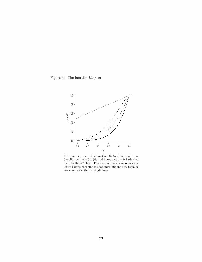
Figure 4: The function Un(p, c)
0.5 0.6 0.7 0.8 0.9 1.0
0.0
0.2
0.4
0.6
0.8
1.0
p
U_n
(p, c
)
The figure compares the function Mn(p, c) for n = 9, c =0 (solid line), c = 0.1 (dotted line), and c = 0.2 (dashedline) to the 45◦ line. Positive correlation increases thejury’s competence under unanimity but the jury remainsless competent than a single juror.
29