Optimal capital requirements over the business andfinancial cycles∗

Frederic Malherbe (London Business School)

July 4, 2017

Abstract

I study economies where banks do not fully internalize the social costs of their lend-

ing decisions. In equilibrium, this leads to over-investment by firms. The bank capital

requirement that restores investment efficiency depends on the state of the economy. I

identify a general equilibrium effect that has two main implications for this optimal capital

requirement. First, it is increasing in aggregate bank capital. Second, it is tighter during

booms than in recessions. A suboptimal policy that overlooks this effect exacerbates eco-

nomic fluctuations as it allows for excessive build-up of risk by banks during booms, and

contracts credit excessively in recessions.

1 Introduction

It is widely acknowledged that financial institutions have incentives to take on too much risk(Kareken and Wallace (1978), Acharya and Richardson (2009)) and that banking crises arecostly for society.1 Until the 2007-2009 global financial crisis, the main focus of bank pru-dential regulation was to contain risk taking at the individual bank level. Ever since, the focus∗I am grateful to Xavier Freixas, Anton Korinek, Marcela Lucchetta, David Martinez-Miera, Marcus Opp,

Jaume Ventura, Lucy White, and Tanju Yorulmazer for their insightful discussions of the paper, to Saleem Ba-haj, Patrick Bolton, Nuno Coimbra, Martin Eichenbaum, Emmanuel Farhi, Alessandro Graniero, Felipe Iachan,Enrique Mendoza, Matthias Paustian, Romain Ranciere, Helene Rey, Jean-Charles Rochet, Wolf Wagner, andseminar and conference participants at or in Amsterdam, Antwerp, the Bank of England, the Bank of Portugal, theBanque de France, Boston University, Cambridge, CREI, ECB, Exeter, Federal Reserve Board, FGV Rio, FGVSao Paulo, Frankfurt, Georgetown, Gerzensee, HSE Moscow, IMF, Konstanz, Lancaster, KU Leuven, LondonBusiness School, London School of Economics, Manchester, the National Bank of Belgium, the New York Fed,Queen Mary, San Diego, the Sveriges Riksbank, Toulouse, Tilburg, Universitat Pompeu Fabra, Warsaw, Warwick,York, and Zurich for their comments and suggestions. This paper has been prepared by the author under the Lam-falussy Fellowship Program sponsored by the ECB. Any views expressed are only those of the author and do notnecessarily represent the views of the ECB or the Eurosystem.

1For instance, the Savings and Loan crisis officially cost the US taxpayer at least $132bn (in 1995 USD). Thereis no consensus on the 2007-2009 crisis’ net fiscal costs, but Laeven and Valencia (2012) estimate the net outlaysat 2.1% of GDP in the US, 6.6% in the UK, up to a vertiginous 40% in Ireland. Besides fiscal costs, banking crisesappear to severely affect the real economy as they are typically followed by long and painful recessions (Jordà,Schularick and Taylor (2013)) and are associated with large permanent output losses (Cerra and Saxena (2008)).

1

has evolved towards containing system-wide risk taking. What are the the costs and benefitsof such policies? What are the relevant general equilibrium effects to take into account? Is anoptimal policy time-varying?

To address such questions, I develop a simple theory of intertwined business and financialcycles, where financial regulation both optimally responds to and influences the business cycle.In the economies I study, regulation is needed because banks do not fully internalize the socialcosts associated with their lending decisions. They do not internalize these costs for two mainreasons. First, in the case of a crisis, some of the costs are ultimately borne by the taxpayer.Second, credit expansion by a bank increases the probability of default of other banks andthe losses they make in such an event. As a result, the competitive equilibrium is generallyinefficient: banks lend too much, which translates into excessive real investment by firms in ageneral equilibrium.

The main focus of the paper is on the time-varying bank capital requirement that restoresinvestment efficiency. The first key contribution of the paper is to highlight a general equilib-rium effect that is a key driver of this optimal capital requirement, and of its cyclical properties.The second is to provide a detailed analysis of the pecuniary externalities generated by thisgeneral equilibrium effect.

The model involves overlapping generations of risk-neutral savers and bankers. Bankersare protected by limited liability. They collect deposits and competitively lend to firms, whichoperate a risky constant returns-to-scale production function. Some firms succeed, some fail.Those that fail default on their bank loan. Banks are perfectly diversified and their realizedreturn to lending depends on the firm default rate. The return to lending also depends on theequilibrium in the labor and capital markets. Labor supply is fixed, so there are diminishingreturns to physical capital, which translates into decreasing marginal returns to lending in ageneral equilibrium. When the proceeds from lending are insufficient to repay depositors infull, the bank is insolvent and defaults, which generates deadweight losses.

To set up the analysis, I establish the market failure and show that the regulator can restoreinvestment efficiency thanks to a time-varying capital requirement. I then study the cyclicalproperties of this optimal capital requirement in two steps. First, I present two simple casesthat can be solved analytically. This allows me to formally identify the main mechanisms atplay. Second, I calibrate the model and solve it numerically to assess the quantitative relevanceof these mechanisms.

I find that the optimal capital requirement is increasing in aggregate bank capital. To seethe intuition, first consider an atomistic bank that doubles its equity. It should simply be allowedto double lending. However, if all banks in the economy double their equity, and if they areallowed to double lending, this could double investment in the economy. Given diminishingreturns to capital this cannot be optimal in a general equilibrium. In fact, the optimal policy isto let the banking sector expand, but less than proportionally, which corresponds to an increasein the capital requirement. This is a central result of the paper.

2

In this economy, aggregate productivity evolves over time. When it is high, the return tolending is high and new bankers also enter the sector with higher wealth (which comes fromtheir wage). Hence, aggregate bank capital is high. Due to the general equilibrium I have justdescribed, this calls for a tightening of the capital requirement. I refer to this effect as the bank

capital channel.When productivity is high, future productivity is likely to be high too. Hence, the firm de-

fault rate is likely to be low, which means that expected lending profitability is high. Efficiencytherefore requires an expansion of aggregate lending. All other things equal, this calls for aloosening of the capital requirement. I refer to this effect as the loan default rate channel.

These two channels pull in opposite directions. My analytical results indicate that the bankcapital channel is stronger than the loan default rate channel. As a result, the capital requirementis tighter during booms than in downturns. Since the bank capital channel is driven by thegeneral equilibrium effect, these analytical results suggest that this effect could be important.

I calibrate the general model and solve it numerically. Simulation results confirm the an-alytical insights. First, I consider the economy at steady state and study the response of theoptimal capital requirement to a single positive shock (namely, a 1% decrease in the loan de-fault rate). This response is positive: the optimal requirement increase peaks around 20bpsafter a few periods and then decays over time. Second, I simulate a full series of shocks. I findthat the optimal capital requirement is higher in good times (i.e. when the loan default rate is atleast one standard deviation below its mean) than in bad times (when the default rate is at leastone standard deviation above its mean).

To explore further the quantitative relevance of the general equilibrium effect, I also com-pare the optimal capital requirement to a suboptimal policy that takes into account the defaultrate channel but ignores the bank capital channel. Under this suboptimal policy, the cyclicalproperties of the requirement are reversed: it is tighter in bad times than in good times. As aresult, banks take on too much risk in good times (they lend too much and retain less profit) andcredit contraction is unnecessarily severe in bad times. According to my calibration, the asso-ciated welfare losses amount to 0.04% of steady state consumption, which is in the ballpark ofnumbers found in the literature on stabilization policy (Lucas, 2003).

The features of the suboptimal policy resonate with the criticisms of the second regimeof the international standards for banking regulation (BCBS (2004)), commonly referred to asBasel II. I show that my framework can easily be extended to study the cyclical effects of therisk-weights that this regime introduced. Then, taking the cyclical effect of risk-weights asgiven, I use my calibration results to compute back-of-the-envelope estimates for the optimaltime-varying adjustments that would restore investment efficiency. I relate these adjustments tothe macroprudential adjustments introduced by Basel III, the current regulatory regime (BCBS(2010)).

It is is well understood that a regulatory regime like Basel II is likely to magnify the business

3

cycle (Kashyap and Stein (2004), Repullo, Saurina and Trucharte (2010)).2 Adjusting capitalrequirements to the aggregate state of the economy seems a sensible response. However, howsuch adjustments should be designed and, more generally, what are their general equilibriumconsequences remain open questions.

Kashyap and Stein (2004) argue in favor of adjustments based on the scarcity of aggregatebank capital (relative to lending opportunity). They point out that a priori it is not obvious thataggregate bank capital scarcity is greater during a recession, but they interpret the empiricalliterature on bank capital crunches as generally supporting such a notion. My theoretical modeldelivers such a result.3 Repullo and Suarez (2013) find, however, the opposite. They study atheoretical model of optimal bank capital requirements and compare them to Basel I, II, andIII. In their setup, even though bank capital is scarcer in bad times, capital requirements shouldstill optimally be tighter than in good times. An important feature of their model is that theproduction function is linear in investment, which explains why they do not capture the generalequilibrium mechanism that drives the result in my model.

Martinez-Miera and Suarez (2014) propose a model where correlated risk-shifting by somebanks gives an incentive to other banks to play it safe. The reason is that banks that survive acrisis earn large scarcity rents in the aftermath, an application of the “last-bank-standing effect”(Perotti and Suarez (2002)). They focus on the optimal level of a constant capital requirement.4

Also, they do not consider business cycle dynamics but, in their model, loosening capital re-quirements after a banking crisis mitigates rents ex-post and induces more systemic risk-takingex ante. In contrast, in Dewatripont and Tirole (2012), incentives to gamble for resurrectionare stronger after a negative macroeconomic shock. In the same vein, Morrison and White(2005) study a model with both moral hazard and adverse selection. They find that the appro-priate policy response to a crisis of confidence may be to tighten capital requirements. Thishappens when the regulator’s ability to alleviate adverse selection through banking supervisionis relatively low.

In Section 5, I dissect the pecuniary externalities associated with the general equilibriumeffect. I show how they interact with bank default costs to generate inefficiencies. I highlight

2Basel I (BCBS (1988)) imposed a capital requirement of 8% on risk-weighted bank assets. Risk weightswhere essentially fixed (there were five coarse categories of borrowers, and borrowers would not change cate-gories). To better with risk heterogeneity in the cross-section, Basel II (BCBS (2004)) introduced risk weightsthat are directly linked to each loan probability of default. But probabilities of default tend to co-move over theeconomic cycle, which created effects in the time-series. In particular, lower probabilities of default in goodtimes decreased the effective stringency of the requirement (and conversely in a bust). If the purpose of capitalrequirement is to contain bank risk-taking, effectively tighter requirements in bad times seems desirable. But bankcapital (equity in the banking sector) is likely to be scarcer in bad times (because banks have incurred losses),which implies a credit contraction in the economy. The consensus is that such a contraction is excessive from asocial point of view.

3In a static model, Repullo (2013) finds that capital requirements should be loosened after an exogenousnegative shock to bank capital. This is in line with Kashyap and Stein (2004)’s premise and with my results, butthe mechanism is different.

4Other recent papers focusing on the optimal level include Morrison and White (2005), Van den Heuvel (2008),Admati et al. (2010), Harris, Opp and Opp (2015), and Begenau (2015).

4

two main classes of externalities. The first, already mentioned above, works through banks’probabilities of default. Credit expansion by a given bank increases aggregate physical capitalin equilibrium and, therefore, decreases its marginal productivity. This, in turn, decreases thereturn to lending of other banks and increases the probability that they default and incur defaultcosts. When making its lending decision, a bank takes its own default costs into account, butnot those of others, which leads to inefficiently high levels of lending. The second class of ex-ternalities works through the banks’ costs given default. Whether these externalities contributeto under- or overlending depends on the specific form of the default cost function. This lastresult directly speaks to the financial accelerator literature (e.g., Bernanke and Gertler (1989);Bernanke, Gertler and Gilchrist (1999); Carlstrom and Fuerst (1997)). More generally, thisanalysis contributes to the literature on externalities in macro-finance models (see Davila andKorinek (2017) for a synthesis).5

The paper is organized as follows: I present and discuss the environment in Section 2. Iestablish the market failure and derive the optimal regulatory response in Section 3. I study thecyclical properties of the optimal capital requirement in Section 4; and I analyze and discussthe externalities in Section 5; I discuss the key ingredients of the model in Section 6; and thenconclude.

2 The baseline model

There is an infinite number of periods indexed by t = 0,1,2..., in which a single consumptiongood is produced and used as the unit of account, and where generations of agents born atdifferent dates overlap.

Agents All agents are risk neutral, live two periods, and derive utility from their end-of-lifeconsumption. There is a measure 1 of agents born at the beginning of each period. They areendowed with one unit of labor, which they supply inelastically during the first period of theirlife. After having worked and received their wage, a measure η 1 of these agents becomeendowed with banking ability, which enables them to set up a bank under the protection oflimited liability. The remaining mass 1−η of agents become passive savers.

To transfer their wealth across periods, all agents have access to a safe storage technologyand bank deposits.6 The rate of return to storage is normalized to zero. I focus on caseswhere the storage technology is used in equilibrium, so that the return to storage pins down theexpected return on deposits.7 In addition, bankers can invest their wealth in their bank’s equity.

5On fire-sales externalities and other amplification mechanisms, see for instance Shleifer and Vishny (1997),Gromb and Vayanos (2002), Krishnamurthy (2003), Lorenzoni (2008), Bianchi (2011), Jeanne and Korinek(2010), Goodhart et al. (2012), Gersbach and Rochet (2012), and Stein (2012), and on aggregate demand ex-ternalities see Farhi and Werning (2013), Rognlie, Shleifer and Simsek (2014), and Korinek and Simsek (2016).

6The economy can be considered as a small open economy with excess savings, facing the world interest rate.7Alternatively, I could simply allow banks to raise deposits from the rest of the world.

5

Banks There is a continuum of banks that issue deposits to savers and lend competitively tofirms. The rate of return to lending is denoted r . It is a random variable, whose distributionis determined in equilibrium, and taken as given by bankers. When a bank’s proceeds fromlending are not sufficient to repay its deposits, the bank defaults. In case of bank default, thegovernment compensates depositors for any loss they made. Hence, deposits pay a zero interestrate. The government does not charge an insurance premium ex-ante but, when needed, levieslump-sum taxes on savers in order to break even in each period.

Bank default generates deadweight losses, which I model as a reduction in the value re-couped by creditors. These deadweight losses can capture a number of situations (e.g. costlystate verification, deadweight losses from taxation generated by an associated bailout, or otherforms of spillovers to the real real economy). Throughout the paper, I will consider several lossfunctions and discuss their interpretations.

Firms In each period, there is a continuum of penniless firms, indexed by i, that operate aconstant-return-to-scale production function. Firms competitively hire labor and borrow frombanks to invest in capital. For simplicity, firms operate only one period and capital can cost-lessly be transformed one for one into consumption good, and vice versa. The productionfunction takes the form ai kαi n1−α

i , where ni denotes labor, ki is physical capital (0 < α < 1), andai ∈ 0,1 is a random variable that captures firm specific productivity.

The realization of ai is observed by firm i at no cost, but is costly to observe for the banks.As is standard, I assume that such verification costs materialize as a reduction in the liquidationvalue of the firm. As a result, the optimal contract is a debt contract, whereby the firm repaysthe principal plus a given interest rate r l when ai = 1, and enters bankruptcy when ai = 0. Toformalize bankruptcy costs, I follow Martinez-Miera and Suarez (2014) and assume that whilecapital depreciates at a rate δ when ai = 1, it depreciates at a larger rate δ +∆ when ai = 0.Finally, I assume that default is independent across firms and denote A ≡ E[ai] the commonlyknown probability that a given firm succeeds.

Shocks To trigger fluctuations in this economy, I let A evolve according to an AR(1) process:

ln At = (1− ρ) ln A+ ρ ln At−1+ ε t , (1)

where ρ is a positive parameter capturing the persistence of the shocks, A is a positive constant,and ε t represents an iid shock with mean zero and standard deviation σ. The realization of At

is the event that defines the beginning of period t.

6

3 Market failure and constrained efficiency

3.1 Competitive equilibrium

The problem of the banker Bankers’ relevant decisions are how to allocate their wealthbetween storage and bank equity and how much the bank lends, given its level of equity. Thiscan be formalized as follows.

Consider a representative bank at date t, and denote by et its amount of equity. To lend anamount bt , the bank needs to raise bt − et of deposits. Let vt+1 denote the ex-post net worth ofthe bank, i.e. its value after its return to lending rt+1 is realized. That is,

vt+1 ≡ btrt+1+ et −Ψt+1

where Ψt+1 is the function that captures the deadweight losses from bank default.Then, consider a representative banker born at date t that has earned a wage wt . He solves:

maxet ,bt

Et [ct+1] (2)

subject to the budget constraints and non-negativity conditions:

et + st = wt

ct+1 = v+t+1+ st

et , bt , st , ct+1 ≥ 0 ,

(3)

where ct+1 represent his consumption, st is the amount he stores from date t to date t + 1, andv+t+1 is the realized (private) value of his bank’s equity, i.e. the positive part of vt+1:

v+t+1 ≡ [btrt+1+ et]+ . (4)

Note that Ψt+1 does not appear in (4) because it is nil when btrt+1+ et ≥ 0 (and positive other-wise).

Labor market Labor is hired at the beginning of the period. That is, after At is known, butbefore ait’s are realized. The labor market is competitive. The expected wage is:8

wt = (1−α) At kαt8At failed firms, the realized wage is nil. This is unrealistic but, since agents are risk neutral, this is the expected

wage that matters. An alternative would be to assume that firms are paid in advance of production (this wouldrequire the firm to borrow additional funds).

7

The return to lending At the end of a given period t − 1, firms borrow competitively frombanks to form capital that they will use for production in period t. Hence, investment takesplace before At is known.

In a competitive equilibrium, the expected unit repayment to the bank equates the firms’expected marginal return to capital (accounting for bankruptcy cost). Since firms are pennilessand protected by limited liability, there cannot be states in which they make strictly positiveprofits (otherwise they would make profits in expectation). As a result, in an optimal contract,the date-t repayment to the bank by a firm i that had borrowed kit and hired nit workers, mustcorrespond to its realized net share of capital. That is:

αkαit n1−αit + (1− δ)kit ; ait = 1

(1− δ−∆) kit ; ait = 0.

Date t−1 capital market clearing requires kt ≡∫

i kit = bt−1, and date t labor market clearingrequires nt ≡

∫i nit = 1. Given constant return to scale, all firms have the same capital to labor

ratio in equilibrium. A standard debt contract with an interest rate r lt ≡ αkα−1

t − δ is thereforeoptimal. Accordingly, the realized rate of return to lending for the bank corresponds to theaverage net marginal return to capital. That is:

r (At ,kt ) = αAt kα−1t − (δ+ (1− At )∆) .

Competitive equilibrium definition Given a sequence for the random variables At ∞t=0, and

initial condition k0, a competitive equilibrium is a sequence wt ,r lt ,et ,bt ,τt

∞t=0, such that: vector

wt ,r lt clears the labor and capital markets at date t and t−1 respectively; vector et ,bt solves

the maximization problem of the representative banker born at date t and τt is a lump-sum taxon savers such that the regulator breaks even at all t.

3.2 Efficiency analysis

Investment efficiency Economic surplus in this economy corresponds to output net of depre-ciation and bank default costs. Formally economic surplus at date t +1 is given by:

S(At+1,kt+1,et ) ≡ At+1kαt+1− (δ+ (1− At+1)∆)) kt+1−Ψ (At+1,kt+1,et ) . (5)

Investment efficiency requires to maximize expected economic surplus. Define:

k∗t+1 ≡ argmaxkt+1

Et [S(At+1,kt+1,et )] (6)

Definition 1. Investment at date t is efficient if and only if kt+1 = k∗t+1.

I can now compare the competitive equilibrium investment level, which I denote kCEt+1, with

8

this efficiency benchmark (which I discuss at the end of this section).

Proposition 1. At all dates, the competitive equilibrium capital stock is inefficiently high. That

is: kCEt+1 > k∗t+1,∀t.

Proof. All the proofs are in Appendix A.

Because of deposit insurance, banks do not fully internalize the losses that occur in badstates. This reflects an implicit subsidy. Banks compete for lending to firms and pass thissubsidy onto the firms in a general equilibrium. As a result, firms over invest. In this context,mispriced deposit insurance is a sufficient ingredient to obtain over-investment, but it is notnecessary. This is because credit expansion by a bank also increases the probability of defaultof other banks and the losses they make in such an event. This externality also operates througha general equilibrium effect and also leads to over-investment, even in the absence of depositinsurance. I postpone the detailed study of these externalities to Section 5 to directly turn to themain object of this analysis: the cyclical properties of the optimal regulatory response.

3.3 Regulatory response and constrained equilibrium

The regulator I study the problem of a regulator, whose mission is to restore investmentefficiency. The regulatory tool is a time-varying capital requirement xt ∈ [0,1] that constrainsbanks’ lending to a multiple of their equity.

et ≥ xt bt . (7)

Henceforth, I refer to et as bank capital.

Constrained equilibrium A constrained equilibrium is defined as a straightforward exten-sion of the competitive equilibrium. Given the same sequence of random variables and initialcondition, it is defined as a sequence of capital requirements xt

∞t=0 and a vector sequence

wt ,r lt ,et ,bt ,τt

∞t=0 satisfying the same conditions, with the only difference that et ,bt must

solve the problem of the representative banker born at t subject to the capital requirement xt .

The optimal capital requirement I restrict my analysis to the interesting case where bankcapital is scarce (i.e. ηtwt < k∗t+1) at all dates t. If bank capital was plentiful, the optimal capitalrequirement would be xt = 1, and banks would be fully funded with equity and could not defaultin equilibrium.9

9See S. Hanson, A. Kashyap and J. Stein (2011), Stein (2012), and Admati et al. (2010) for discussions on whybank capital is scarce in reality.

9

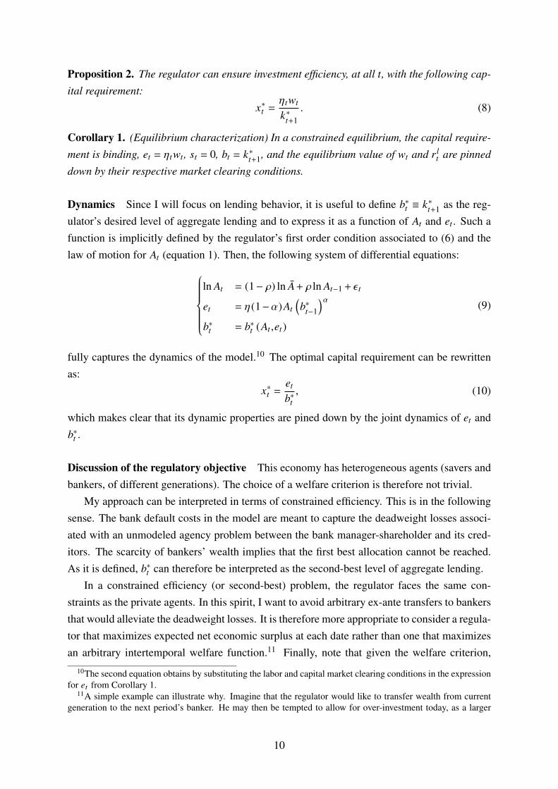
Proposition 2. The regulator can ensure investment efficiency, at all t, with the following cap-

ital requirement:

x∗t =ηtwt

k∗t+1. (8)

Corollary 1. (Equilibrium characterization) In a constrained equilibrium, the capital require-

ment is binding, et = ηtwt , st = 0, bt = k∗t+1, and the equilibrium value of wt and r lt are pinned

down by their respective market clearing conditions.

Dynamics Since I will focus on lending behavior, it is useful to define b∗t ≡ k∗t+1 as the reg-ulator’s desired level of aggregate lending and to express it as a function of At and et . Such afunction is implicitly defined by the regulator’s first order condition associated to (6) and thelaw of motion for At (equation 1). Then, the following system of differential equations:

ln At = (1− ρ) ln A+ ρ ln At−1+ ε t

et = η(1−α) At(b∗t−1

)αb∗t = b∗t (At ,et )

(9)

fully captures the dynamics of the model.10 The optimal capital requirement can be rewrittenas:

x∗t =et

b∗t, (10)

which makes clear that its dynamic properties are pined down by the joint dynamics of et andb∗t .

Discussion of the regulatory objective This economy has heterogeneous agents (savers andbankers, of different generations). The choice of a welfare criterion is therefore not trivial.

My approach can be interpreted in terms of constrained efficiency. This is in the followingsense. The bank default costs in the model are meant to capture the deadweight losses associ-ated with an unmodeled agency problem between the bank manager-shareholder and its cred-itors. The scarcity of bankers’ wealth implies that the first best allocation cannot be reached.As it is defined, b∗t can therefore be interpreted as the second-best level of aggregate lending.

In a constrained efficiency (or second-best) problem, the regulator faces the same con-straints as the private agents. In this spirit, I want to avoid arbitrary ex-ante transfers to bankersthat would alleviate the deadweight losses. It is therefore more appropriate to consider a regula-tor that maximizes expected net economic surplus at each date rather than one that maximizesan arbitrary intertemporal welfare function.11 Finally, note that given the welfare criterion,

10The second equation obtains by substituting the labor and capital market clearing conditions in the expressionfor et from Corollary 1.

11A simple example can illustrate why. Imagine that the regulator would like to transfer wealth from currentgeneration to the next period’s banker. He may then be tempted to allow for over-investment today, as a larger

10

Proposition 2 establishes that focusing on capital requirements is not restrictive since it allowsto restore efficiency at all dates.

4 Cyclical properties of the optimal capital requirement

In this Section I study the dynamic properties of x∗t . First, I identify a key general equilibriumeffect that drives the contemporaneous effect of et on x∗t . Then, I use two simple examples toidentify and disentangle the main mechanisms by which productivity shocks propagate overtime. Then, I calibrate and solve numerically the general model to assess the quantitativerelevance of these mechanisms.

Default cost function For this part of the analysis, I consider a simple default cost functionwhere deadweight losses are proportional to the representative bank’s financial distress. Thatis, they are proportional to the extent to which the net worth of the bank is negative. Formally:

Ψt+1 ≡ γ [− (btrt+1+ et )]+ , (11)

where γ is a positive parameter, operator [ . ]+ selects the positive part of the argument, andbtrt+1+ et the realized net worth. Hence, by construction, the costs only occur when net worthis negative, that is, when the bank defaults.

There are several possible interpretations for such a specification. For now, to fix ideas, itis useful to think of deadweight losses as emanating from the bank resolution process, which isarguably longer and more complicated when financial distress is high. Besides being intuitivelyappealing, default cost function (11) is analytically convenient (Townsend, 1979). However, themain results do not hinge on this specification (see Section 5 for alternative specifications anda full discussion).

4.1 The general equilibrium effect

A key contribution of this paper is to highlight a simple, but nonetheless important, generalequilibrium effect. To isolate this effect, it is useful to consider exogenous shocks to aggregatebank capital. To do so, I fix At and express x∗t as a function of et :

x∗t (et ) =et

b∗t (et ).

It is clear that x∗t (et ) is an increasing function unless b∗t increases more than proportionally withet . Denoting κt the point elasticity of b∗t with respect to et , I can state the following result.

capital stock will boost tomorrow’s wage and, therefore, the wealth of future bankers. This involves negativenet-present-value investment, but the regulator could still find it desirable given its objective functions and theconstraints it faces.

11

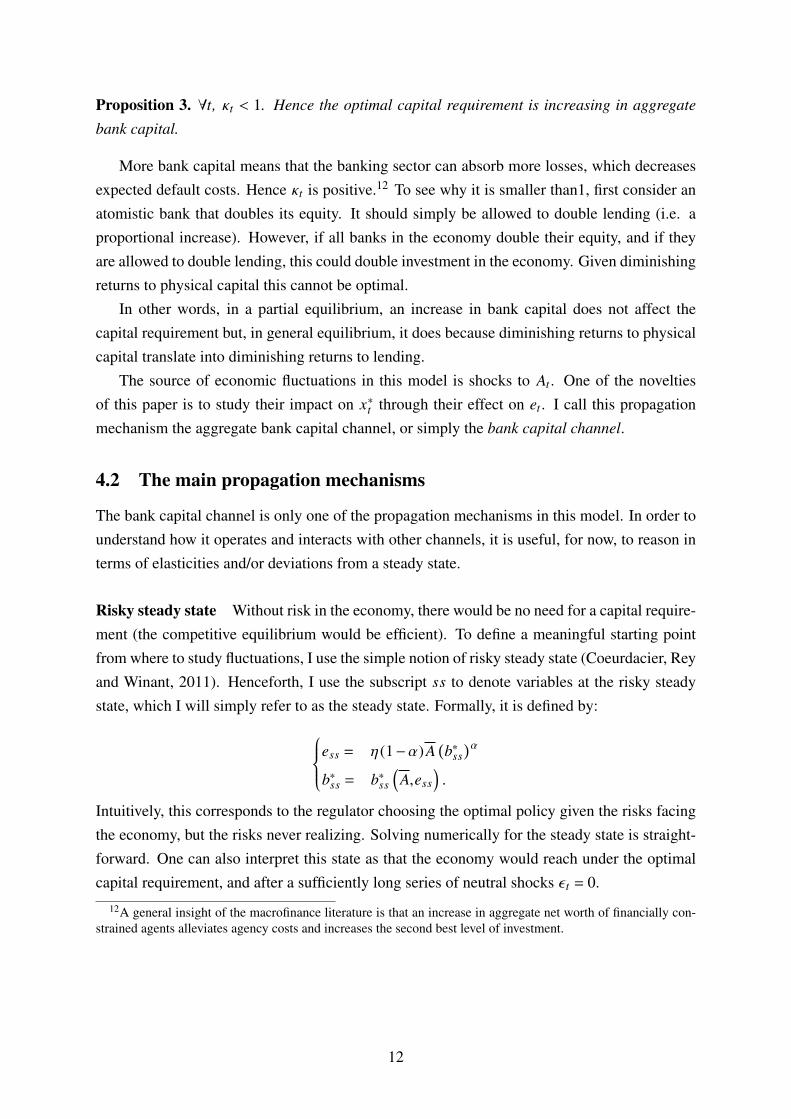
Proposition 3. ∀t, κt < 1. Hence the optimal capital requirement is increasing in aggregate

bank capital.

More bank capital means that the banking sector can absorb more losses, which decreasesexpected default costs. Hence κt is positive.12 To see why it is smaller than1, first consider anatomistic bank that doubles its equity. It should simply be allowed to double lending (i.e. aproportional increase). However, if all banks in the economy double their equity, and if theyare allowed to double lending, this could double investment in the economy. Given diminishingreturns to physical capital this cannot be optimal.

In other words, in a partial equilibrium, an increase in bank capital does not affect thecapital requirement but, in general equilibrium, it does because diminishing returns to physicalcapital translate into diminishing returns to lending.

The source of economic fluctuations in this model is shocks to At . One of the noveltiesof this paper is to study their impact on x∗t through their effect on et . I call this propagationmechanism the aggregate bank capital channel, or simply the bank capital channel.

4.2 The main propagation mechanisms

The bank capital channel is only one of the propagation mechanisms in this model. In order tounderstand how it operates and interacts with other channels, it is useful, for now, to reason interms of elasticities and/or deviations from a steady state.

Risky steady state Without risk in the economy, there would be no need for a capital require-ment (the competitive equilibrium would be efficient). To define a meaningful starting pointfrom where to study fluctuations, I use the simple notion of risky steady state (Coeurdacier, Reyand Winant, 2011). Henceforth, I use the subscript ss to denote variables at the risky steadystate, which I will simply refer to as the steady state. Formally, it is defined by:

ess = η(1−α)A(b∗ss

)αb∗ss = b∗ss

(A,ess

).

Intuitively, this corresponds to the regulator choosing the optimal policy given the risks facingthe economy, but the risks never realizing. Solving numerically for the steady state is straight-forward. One can also interpret this state as that the economy would reach under the optimalcapital requirement, and after a sufficiently long series of neutral shocks ε t = 0.

12A general insight of the macrofinance literature is that an increase in aggregate net worth of financially con-strained agents alleviates agency costs and increases the second best level of investment.

12

Elasticities Defining at as the log-deviation of At from A, we have that if the economy is atsteady state at date 0:

at =

t∑s=1

ρt−1ε t . (12)

In Subsection 4.3, I analyze the model globally. But for now, let me focus on system (9)linearized around the steady state. Together with (12), we have:

et = at +αbt−1

bt = ξat + κet

xt = et − bt

(13)

where bold variables et , bt , and xt are the log-deviation from ess, b∗ss, and x∗ss. Finally, ξ andκ are the point elasticity of b∗ss with respect to At and et . In the two examples that follow, Iconsider the effect of a unique initial productivity shock, starting from steady state. That is:ε1 = 1 and ε t,1 = 0.

4.2.1 The bank capital channel

Let me consider a first example where At are iid (i.e. ρ= 0). In this case, expected productivityis constant at all time. Hence, ξ = 0, and

xt = et (1− κ).

The only effect at play is the bank capital channel identified above. In fact, here, ε t can beinterpreted as a financial shock, in the sense that it affects the wealth that flows into aggregatebank capital, which impacts banking sector’s intermediation capacity, without having othereffects on k∗t+1.

From Proposition 3, we know κ < 1 . Hence, the immediate response to the shock is totighten the capital requirement:

x1 = (1− κ).

In subsequent periods, there is a feedback effect as et increases with bt−1 (more lending meansmore capital, which raises the equilibrium wage and, therefore, future bank capital). Iteratingforward, I can solve system (13) for xt :

xt = (ακ)t (1− κ),

which shows that the response is positive at all t and allows me to unambiguously sign the bankcapital channel: through it, a positive shock increases the optimal capital requirement.13

13If ρ > 0, the bank capital channel is reinforced because productivity is persistently raised. This boosts wages,which in turn increases future bank equity.

13

4.2.2 The loan default rate channel

In a second example, I assume away default costs in the banking sector (γ = 0). In this caseeconomic surplus (5) no longer depends on et , and one can solve for b∗t in closed form:

b∗t =(

αEt[At+1]δ+ (1−Et[At+1])∆

) 11−α

. (14)

This expression makes clear that b∗t is increasing in At (strictly when ρ > 0). The intuitionis simple: a positive productivity shock raises expected productivity, which calls for moreinvestment, which requires more lending.

In terms of elasticities, this means that ξ > 0. Looking at the second equation of system(13), we can see that this effect operates through the term ξat . Reinterpreting this channel froma bank lending standpoint, an increase in At decreases the loan default rate. This makes lendingmore profitable in expectation and calls for an expansion in aggregate lending. I refer to thismechanism as the loan default rate channel, or simply the default rate channel.

4.2.3 Which channel is likely to dominate?

The bank capital channel and the default rate channel pull in opposite directions. To get a firstsense of their relative importance, I assume further that ∆ = 0. This is useful because equation(14) then boils down to an isoelastic function, which gives:

ξ =ρ

1−α.

In this case, the immediate response to the shock is:

x1 = 1−ρ

1−α.

This means that x1 < 0, unless ρ < 1−α. Hence, unless the shock has relatively low persistence,the immediate optimal response to a positive shock is to loosen the requirement.

Feedback effect However, any increase in b∗t raises kt+1,which boosts wages and, therefore,increases et+1. Looking at the second equation of system (13), we can see that this effectoperates through the term αbt−1. Since γ = 0 implies κ = 0, we get:

xt = at + ξαat−1︸ ︷︷ ︸feedback effect︸ ︷︷ ︸

bank capital channel

− ξat︸︷︷︸default rate channel

,

Hence:xt>1 = ρ

t−1(

1− ρ1−α

)> 0,

14

which means that the feedback effect is sufficient to ensure that xt>1 is always positive. I collectthese results in a formal proposition.

Proposition 4. Assume default is costless (γ = 0 and ∆ = 0). The bank capital channel domi-

nates the default rate channel at any positive lag. In the period where the shock occurs, this is

true if the shock is not too persistent. Formally, following a date-1 positive productivity shock,

E1[xt>1] > 0, and x1 > 0⇔ ρ < 1−α.

In sum, in this example, aggregate bank capital is more procyclical than the efficient levelof the capital stock. This suggests that the optimal capital requirement increases during booms.Since the positive effect comes from the bank capital channel, this also suggests that the generalequilibrium that drives it could be quantitatively important.

4.3 Intertwined business and financial cycles

In the subsection above, I have highlighted the main propagation mechanisms. An increase inproductivity raises x∗t through the bank capital channel, but it decreases it through the defaultrate channels. In the example above (where γ = ∆ = 0), the former effect dominate. In thissubsection, I assess the quantitative relevance of the bank capital channel for the dynamics ofthe general model. That is, I now fully allow for feedback effects and non-linearities.14 I dothis in three steps.

First, I solve the model numerically to generate impulse response functions for x∗t , et , andb∗t . Second, I simulate the economy under x∗t , and compare the outcome to an economy facingan identical series of shocks but using a different policy function x

′

t , which takes into accountthe loan default rate channel but not the bank capital channel. I interpret the difference ineconomic surplus as a measure of the welfare cost of ignoring the general equilibrium effect.Third, I add to the model a reduced-form version of Basel II’s risk-weights and, in the spiritof Basel III, I use my framework to compute back-of-the-envelope estimates for optimal time-varying macroprudential capital buffers.

4.3.1 Methodology

Additional ingredient In real life, retained profits are an important source of capital forbanks. The two-period overlapping generation structure of the baseline model rules out profitretention. This is a useful assumption because it allows for transparent analytical results. Butsince studying the dynamics of x∗ in the general case already requires using numerical methods,I enrich the model in order to allow for such a source of bank capital.

14Compared to the case in Proposition 3, we get at least three additional effects in the general model. First, κ > 0decreases the strength of the bank capital channel. Second, ∆ > 0 affects ξ. And third, there are non-linearities(for instance due to the truncation implied by limited liability).

15

To do so, I use a common modelling trick and impose an exogenous exit rate for banks (seethe discussion in Suarez, 2010). That is, I assume that bankers face a constant probability todie λ, which yields the following condition:

et+1 ≤ ηwt+1+ (1− λ) [btrt+1+ et]+︸ ︷︷ ︸realized net worth

, (15)

where btrt+1 captures the (potentially negative) profit from lending. The case where λ = 1corresponds to the baseline model.

I maintain the assumption that aggregate bank capital is scarce. This is the case in allthe simulations I present in this section. As a result, under the optimal capital requirement,surviving bankers always find it optimal to invest all their wealth in bank equity. This meansthat condition (15) holds with equality and defines the law of motion for aggregate bank capital.

Calibration strategy I interpret one period in the model as 1 year. I choose standard valuesfor the basic technology parameters: α = 0.35 and δ = 0.05. The choice of a value for ∆,the extra depreciation of capital due to default, is less obvious as previous studies have useda relatively wide range of values. As a baseline, I follow Repullo and Suarez (2013) andMartinez-Miera and Suarez (2014) and set ∆ = 0.40. Their rationale for such a value is thatit generates realistic loan losses given default (under Basel II standardized approach, the lossgiven default for non-rated corporate exposure is 45%).15

The exogenous random variable is At , which I express here in terms of loan default rate:Dt ≡ 1− At . The relevant parameters for its distribution are the constant A, and the standarddeviation and persistence of the shocks, σ and ρ. I calibrate these values to match the average(3.9%), the standard deviation (1.9%), and the (annual) autocorrelation (0.83) of the US bankloan delinquency rate from 1985 to 2016.16

This leaves me with three free parameters: λ, η, and γ. The first two are driving aggregatebank capital accumulation. Parameter λ can naturally be linked to the shareholder payout ratio.I choose λ = 0.064, which is the value induced by a payout ratio of 60% ratio for financial firms(Floyd, Li and Skinner 2015) on a 12% return on equity.17 Given this value for λ, I pick thevalue of η to target a bank capital ratio of 4% in the risky steady state, which is in line with

15In my model, the loss given default on a loan (in percent) is equal to δ+∆, hence the value for ∆. The mainalternative approach is to target estimates of bankruptcy costs. For instance, Carlstrom and Fuerst 1997 argue thata reasonable range for estimates that include both the direct and indirect costs is [0.2 to 0.36]. They use a value of0.25. See Subsection 4.4 for a discussion on how this choice and that of other parameter values affect the results.

16Specifically, I use the end of Q4 value of the Delinquency Rate on All Loans, Top 100Banks Ranked by Assets [DRALT100N], retrieved from FRED, Federal Reserve Bank of St. Louis;https://fred.stlouisfed.org/series/DRALT100N, April 3, 2017. I calibrate the parameters to match the momentson a simulated series of 1,000,000 shocks.

17Formally, λ = (Payout Ratio)×ROE/(1+ROE). Note that studies adopting a comparable modelling approachtypically use higher values for the corresponding parameter, which they link to average survival time for firms orbanks (e.g, the exit rate is 0.1 in Gertler and Kiyotaki (2010) and 0.11 in Bernanke, Gertler and Gilchrist, 1999,and 0.2 in Martinez-Miera and Suarez (2014)).

16

average leverage ratios for banks in the decade before the global financial crisis (Adrian andShin, 2010). Note that given a typical average risk-weight below 50%, this allows to satisfythe Basel II risked weighted capital ratio of 8%. The last parameter (γ) is specific to mymodel and captures the intensity of bank default costs. In the absence of empirical estimates, Iconsider several values, ranging from 0 to 4. I use γ = 2 as a baseline, which yields a simulateddeadweight loss of 5% of steady state GDP, on average, when the representative bank defaults.Table 1 summarizes my calibration strategy.

Table 1: CalibrationValue Target

Concavity of the production function α 0.35 Capital share of outputBaseline depreciation δ 0.05 Physical capital depreciationExtra-depreciation in default ∆ 0.40 Loss given default on bank loansDefault rate parameters Loan delinquency rate (US)Expected success rate A 0.9575 Average (1985-2016): 3.9%Standard deviation of the shock ε σ 0.26 St. dev. (1985-2016): 1.9%Persistence of the shock ε ρ 0.83 Autocorr. (1985-2016): 0.83Banker exit rate λ 0.064 60% payout rate on 12% ROEMeasure of bankers η 0.0212 4% capital ratio (8% of RWA)Bank default cost γ 2 I also consider γ = 0, 1

2 ,4

Note: The default rate parameters are such that the moments of a simulated series of 1,000,000 shocks matchthose of the loan delinquency rates.

4.3.2 The cyclical properties of the optimal requirement

Figure 1 shows the main impulse response functions for the baseline calibration. Starting fromsteady state, it depicts the effects of a positive productivity shock that decreases the loan defaultrate by 1% (from 4.25% to 3.25%). The left panel displays x∗t , the response of the optimalcapital requirement. It is initially positive (by around 5bps) and reaches 20bps after 8 periodsbefore decaying.

The right panel shows the response of aggregate bank capital and of the efficient level ofaggregate lending. These responses are expressed in percentage deviation from steady state.They are therefore the non-linear counterparts of et and bt . With a slight abuse of notation, Iwill use the same bold letters to refer to these response functions. To link the two panels, notethat x∗t − xss ' (et − bt )xss, where xss = 0.04. Both responses are positive and decay over time.Note that e1 is only slightly larger than b1, but the latter decays at a faster pace, which explainsthe hump shape of x∗t .

The key takeaway from Figure 1 is that it confirms the analytical insights above. In particu-lar: (i) the capital requirement is increasing in aggregate bank capital (as in Proposition 3); and(ii) bank capital is more procyclical than the desired, efficient level of aggregate lending, sothat the optimal response to a positive productivity shocks is to tighten the capital requirement

17

Figure 1: Impulse responses

This figure presents results for the baseline calibration (see Table 1). The left panel shows the path for the optimalcapital requirement x∗t , starting from steady state and following a 1% decrease in the loan default rate. The rightpanel decomposes the response in two parts by showing the impulse responses for aggregate bank capital (blackcircles) and the efficient level of aggregate lending (red dots), expressed in percent deviation from their steadystate values.

Table 2: Simulation results (baseline calibration)Mean x∗t x

′

t

Unconditional 4% 3.9%In good time 4.4% 3.2%In bad times 2.9% 5.4%

This table compares simulated moments under the optimal capital requirement (x∗) and the alternative policy (x′

)defined by equation (16). Both simulations use baseline calibration parameters (Table 1), start at steady state, andfollow the exact same sequence of 10,000 random shocks. Good times (bad times) are defined as periods wherethe loan default rate is at least one standard deviation below (above) the sample mean.

(as in Proposition 4).These results, and their robustness (see Subsection 4.4), provide support for the quantitative

relevance of the bank capital channel and, therefore, of the general equilibrium effect that drivesit.

4.3.3 Good times versus bad times

Figure 1 focuses on fluctuations close to steady state. A simple way to confirm that the maininsights hold globally is to simulate a full series of shocks and compare the simulated optimalrequirement in “good times” versus “bad times”. I define good times (bad times) as periods inwhich the loan default rate is at least one standard deviation below (above) its mean. Table 2displays the simulation results. As we can see, x∗t is indeed tighter in good times (4.4%) thanin bad times (2.9%).

An alternative policy To get a sense of the role of the bank capital channel for the resultsabove, it is useful to define an alternative, suboptimal policy for the the capital requirement.

18

What I want to capture is a policy that takes into account the default rate channel, but ignoresthe bank capital channel. I model such a policy as follows:

x′

t ≡ess

b′t, (16)

whereb′

t ≡ argmaxbt

Et [S(At+1,bt ,ess)] .

That is, b′

t corresponds to the efficient level of aggregate lending if et = ess. This policy ignoresthe bank capital channel in the sense that it holds et constant to its steady state level.18 Thelinearized model of Subsection 4.2 provides a related interpretation: around the steady stateb′

t ' ξat and, therefore,x′

t ' xt − et (1− κ).

Figure 2: Alternative capital requirement policy

This figure presents results for the baseline calibration (see Table 1). The solid black line corresponds the the leftpanel of Figure 1. It is the path for the optimal capital requirement x∗t , starting from steady state and following a1% decrease in the loan default rate. The sequence of blue diamonds depicts the path of the capital requirementpolicy that ignores the bank capital channel (see equation 16).

I compare the response to a positive productivity shock under this policy to the optimalresponse in Figure 2. Ignoring the bank capital channel leads to a loosening of the capitalrequirement instead of a tightening. The difference is initially around 40bps and then decaysover time. Conversely, in case of a negative productivity shock, this policy results in excessivelystringent capital requirements.

The last column of Table 2 shows that the same insights hold away from steady state: x′

t islooser in good times and tighter in bad times. As we will see, policy x

′

t unnecessarily magnifybusiness cycle fluctuations, which resonates with the critiques of the Basel II regulatory regime.Before exploring this further, let me discuss the quantitative role of bank default costs, andpresent further details on the simulation results.

18Note that, by construction, policy x′

t also ignores the feedback effect (i.e. the dependence of et on bt−1).

19

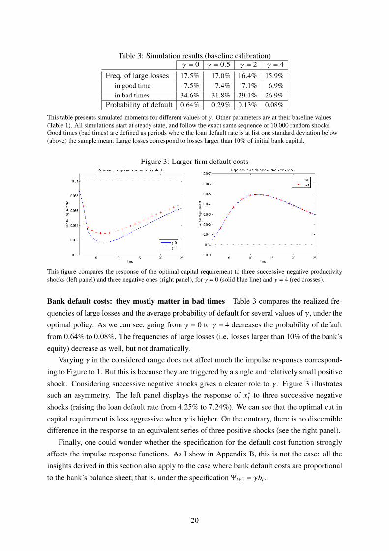
Table 3: Simulation results (baseline calibration)γ = 0 γ = 0.5 γ = 2 γ = 4

Freq. of large losses 17.5% 17.0% 16.4% 15.9%in good time 7.5% 7.4% 7.1% 6.9%in bad times 34.6% 31.8% 29.1% 26.9%

Probability of default 0.64% 0.29% 0.13% 0.08%

This table presents simulated moments for different values of γ. Other parameters are at their baseline values(Table 1). All simulations start at steady state, and follow the exact same sequence of 10,000 random shocks.Good times (bad times) are defined as periods where the loan default rate is at list one standard deviation below(above) the sample mean. Large losses correspond to losses larger than 10% of initial bank capital.

Figure 3: Larger firm default costs

This figure compares the response of the optimal capital requirement to three successive negative productivityshocks (left panel) and three negative ones (right panel), for γ = 0 (solid blue line) and γ = 4 (red crosses).

Bank default costs: they mostly matter in bad times Table 3 compares the realized fre-quencies of large losses and the average probability of default for several values of γ, under theoptimal policy. As we can see, going from γ = 0 to γ = 4 decreases the probability of defaultfrom 0.64% to 0.08%. The frequencies of large losses (i.e. losses larger than 10% of the bank’sequity) decrease as well, but not dramatically.

Varying γ in the considered range does not affect much the impulse responses correspond-ing to Figure to 1. But this is because they are triggered by a single and relatively small positiveshock. Considering successive negative shocks gives a clearer role to γ. Figure 3 illustratessuch an asymmetry. The left panel displays the response of x∗t to three successive negativeshocks (raising the loan default rate from 4.25% to 7.24%). We can see that the optimal cut incapital requirement is less aggressive when γ is higher. On the contrary, there is no discernibledifference in the response to an equivalent series of three positive shocks (see the right panel).

Finally, one could wonder whether the specification for the default cost function stronglyaffects the impulse response functions. As I show in Appendix B, this is not the case: all theinsights derived in this section also apply to the case where bank default costs are proportionalto the bank’s balance sheet; that is, under the specification Ψt+1 = γbt .

20

4.3.4 Comparing policies: further simulation results

Table 5 in Appendix C displays a series of additional results for the comparison between x∗tand x

′

t . Here are the main findings. First, I find that aggregate lending is more volatile under x′

t .Interestingly, the frequency of large bank losses is slightly lower under this suboptimal policy(16% compared to 16.4%). However, distinguishing between good times and bad times givesa nuanced picture. In good times, large losses are more frequent under x

′

t (12.1% compared to7.1% under x∗t ), which is consistent with the popular notion that banks are piling up risks ingood times.19 In bad times, however, banks do not take enough risk under x

′

t as large losses aremuch less frequent than under x∗t (11.8% compared to 29.12%). This is because x∗t optimallytrades off the costs of risk taking with the benefits of allowing for positive net present valueloans to be made. This also explains why the average probability of default is slightly higherunder x∗t .

The excessive risk taking in good times under x′

t materializes in two ways. First, banksdo not fully internalize the social costs of of their credit expansion, which means that theylend too much (see Proposition 1 and Section 5 for further intuition). Second, they do notfully retain their equity.20 This feature resonates with the well-documented dramatic increasein shareholder payouts by banks in the run-up to the global financial crisis (see, e.g., Acharyaet al., 2011 and Floyd, Li and Skinner, 2015).

In the model, the relevant measure of welfare is economic surplus (as defined in Equation(5)). At steady state, it corresponds to aggregate consumption. I find that the average welfareloss associated with x

′

t amounts to 0.04% of steady state consumption. This number is in theballpark of those typically associated with the welfare gains from traditional stabilization policy(see e.g. Lucas, 2003). My model is too stylized to take the results of this exercise at face value,but this simple metric is another hint of the bank capital channel quantitative relevance.

4.3.5 Basel II and the countercyclical buffers of Basel III

The model is useful to think about the so-called procyclical effects of Basel II and countercycli-cal buffers of Basel III.

A Basel II interpretation A key feature introduced by the Basel II regulatory regime is thatbank assets are weighted for capital regulation purposes. The weights on individual loansdepend on their probability of default; either directly (in the “Advanced” or “Internal RatingBased” approach) or through credit ratings (in the “Standardized” approach).

19See Borio and Drehmann (2009) and Boissay, Collard and Smets (2013) for instance.20Under x

′

t , condition (15) may not be binding in equilibrium. This is in that case that banks pay extra dividends.Here, I allow surviving bankers to re-inject equity in the bank in the future, which somehow alleviates the creditcrunch in bad times. In reality, however, banks are typically reluctant to raise capital in bad times, for instancebecause of stigma or debt overhang considerations. Such ingredients involve considerable technical challenges ina dynamic general equilibrium model (see Bahaj and Malherbe (2016)). I therefore leave this to future research.

21

These weights were designed to deal with cross-sectional differences in loan riskiness.However, because probabilities of default co-move over the business cycle, the average, oreffective, risk weight of a given loan portfolio evolves over time. Namely, the effective riskweight goes up during a downturn, and down during a boom. In the context of my model, asimplified version of Basel II’s capital requirement can be captured by the following constraint:

et ≥ xωt bt , (17)

where x is a constant capital requirement (for instance 8% as in the Basel II regime), ωt is theeffective risk weight on the loan portfolio at date t and, as before, et and bt are the representativebank’s capital and lending level. In a more general set-up, the effective risk-weight would bea function of both the portfolio composition (bi’s), and the associated probabilities of default(ai’s) and losses given default (which I could capture by indexing ∆i). However, since onlyaggregate risk matters in my model, the only relevant variable here is the expected loan defaultrate. Accordingly, I define

ωt ≡ ω (Et[Dt+1]) ,

where ω( . ) is an increasing function.

Macroprudential buffers Now, consider a macroprudential regulator that takes as given therules set by a microprudential regulator. In particular, consider a capital constraint that cor-responds to (17) except that the macroprudential regulator can set a time-varying adjustmentfactor zt . That is, consider the capital requirement constraint:

et ≥ zt xωt bt .

Assuming it binds in equilibrium (which implies bt = b∗t ), efficiency requires:

z∗t =et

xωt b∗t. (18)

Log-linearizing around the steady state gives:

zt = et − bt −ωt ,

and the following expression for the optimal macroprudential buffer:

z∗t ' zt x.

Since ω increases with the loan default rate, the response of ωt to a positive productivityshock is negative. Hence, ceteris paribus, this loosens the capital constraint. From a conceptualpoint of view, this is not necessarily a bad thing because higher productivity calls for more

22

investment, which requires more lending. In the context of the model, such a desired increase inlending due to the increase in credit quality can be captured by b

′

t , which leads to the followinginterpretation:

zt ' et (1− κ)︸ ︷︷ ︸bank capital

− b′

t︸︷︷︸credit quality

− ωt︸︷︷︸risk weights

.

As an example, assume that the effect of the change in risk-weights just generates theadjustment required by the change in credit quality. That is, assume ωt = −b

′

t . Then, the onlyrole for the macroprudential buffer is to account for the bank capital channel.

When changes in γ have little effect on xt this means that κ ' 0. From the discussionabove, we now that this is a good approximation in normal and good times. In that case, wehave zt ' et . The baseline impulse response (Figure 1) can then be used in a back-of-the-envelope estimation of the optimal macroprudential buffer. With this approach, the buffer thatcorresponds to a decrease of 1% in the loan default rate is approximately 11%×8% = 88bps att = 0, and then decays over time.

Now, it is widely accepted that the time varying effect of risk weights is excessive. Thereis no empirical consensus on an estimate for the elasticity of ωt with respect to productivity,but a series of studies have attempted to measure such an effect. For instance, using a defaultprobability model, Kashyap and Stein (2004) obtain an implied increase of 10% in risk weightsfrom 1998 to 2002 (a period where the US economy contracted and where, according to thedata I use for the calibration, there was an increase in a bit less than one percent in delinquencyrates).21

Assuming ω4 = −10% and, according to the baseline impulse responses, e4 = 9.7% andb4 = 5.7%, yields

z4 ' 9.7%︸︷︷︸bank capital

− 5.7%︸︷︷︸credit quality

+ 10%︸︷︷︸risk weights

= 14%,

which gives a macroprudential buffer:

z∗4 = 14%×8% = 1.12%

This exercise is very stylized, but it illustrates how the present framework can be usedto think formally about the cyclical effects of risk-weights and the so-called countercyclicalbuffers introduced by Basel III.

4.4 Sensitivity analysis

I have explored the parameter space beyond the set of values of my baseline calibration. Thegeneral conclusion from my numerical analysis is that the shape of the impulse response func-tions and, to some extent, their magnitude are quite robust to alternative parametrizations.

21Other approaches typically give higher numbers. Kashyap and Stein (2004) propose several approaches anddiscuss other estimates found in the literature (see, e.g., Catarineu-Rabell, Jackson and Tsomocos (2005)).

23

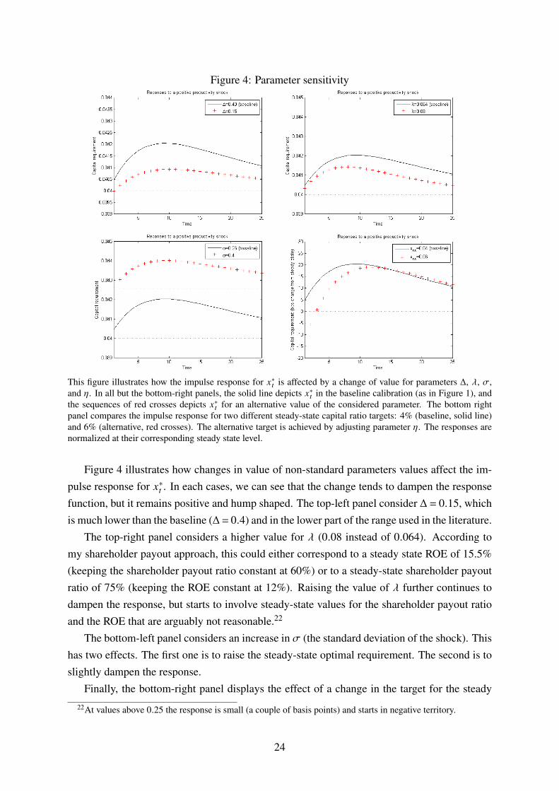
Figure 4: Parameter sensitivity

This figure illustrates how the impulse response for x∗t is affected by a change of value for parameters ∆, λ, σ,and η. In all but the bottom-right panels, the solid line depicts x∗t in the baseline calibration (as in Figure 1), andthe sequences of red crosses depicts x∗t for an alternative value of the considered parameter. The bottom rightpanel compares the impulse response for two different steady-state capital ratio targets: 4% (baseline, solid line)and 6% (alternative, red crosses). The alternative target is achieved by adjusting parameter η. The responses arenormalized at their corresponding steady state level.

Figure 4 illustrates how changes in value of non-standard parameters values affect the im-pulse response for x∗t . In each cases, we can see that the change tends to dampen the responsefunction, but it remains positive and hump shaped. The top-left panel consider ∆ = 0.15, whichis much lower than the baseline (∆= 0.4) and in the lower part of the range used in the literature.

The top-right panel considers a higher value for λ (0.08 instead of 0.064). According tomy shareholder payout approach, this could either correspond to a steady state ROE of 15.5%(keeping the shareholder payout ratio constant at 60%) or to a steady-state shareholder payoutratio of 75% (keeping the ROE constant at 12%). Raising the value of λ further continues todampen the response, but starts to involve steady-state values for the shareholder payout ratioand the ROE that are arguably not reasonable.22

The bottom-left panel considers an increase in σ (the standard deviation of the shock). Thishas two effects. The first one is to raise the steady-state optimal requirement. The second is toslightly dampen the response.

Finally, the bottom-right panel displays the effect of a change in the target for the steady

22At values above 0.25 the response is small (a couple of basis points) and starts in negative territory.

24

state capital ratio (it keeps λ constant and lets η adjust to meet the target). This substantiallyaffects the initial response as it becomes negative. However, the response quickly becomespositive and converges to the baseline case. This pattern is very similar to that described inProposition 4.

5 Dissecting the externalities

Default costs for banks play several roles in the model. As I have shown above, they asymmet-rically affect the optimal response of the capital requirement, with the stronger effect takingplace in bad times. But they also interact with the general equilibrium effect to contribute tothe need for the capital requirement in the first place: as I show in this section, they typicallygenerate externalities that lead to excessive lending in the competitive equilibrium.

5.1 Setting up the problem

Until now, I have assumed that deposits are guaranteed by the government. Not only becausethis is a relevant feature of the environment for real life bank, but also because it simplifiesthe exposition of the main results. In this section, I also consider the case where there are nogovernment guarantees. When there are no government guarantees, if the bank defaults withpositive probability in equilibrium, depositors must be compensated by a higher interest rate inthe states where the bank stays solvent. I denote r ≥ 0 the interest paid on deposits (r = 0 inthe presence of government guarantees). For this part of the analysis, I focus on a single periodand, therefore, omit time subscripts to improve readability.

The default threshold In the general case where r ≥ 0, the representative bank defaults if

(b− e)(1+ r

)> b (1+ r) , (19)

where the left-hand-side is the total promised repayment to depositors and the right-hand-sideis the proceeds from lending.

The equilibrium return to lending is:

r (A,k) = αAkα−1− (δ+ (1− A)∆)) .

Substituting in (19), I can solve for the threshold realization for A below which the representa-tive bank defaults:

A0 ≡

(δ+∆+ r

)b− e(1+ r)(

αkα−1+∆)

b(20)

25

The depositors’ break even condition The break even condition for the depositors reads:∫ ∞

A0

(1+ r) f (A)dA+∫ A0

0

b(1+ r (A))−Ψ(A,r ,b,e,k)b− e

f (A)dA = 0. (21)

The first integral correspond to the states where the bank is solvent and can repay the depositsin full, including the promised interests. The second term, where I now consider a generaldefault cost function Ψ(A,r ,b,e,k), captures what depositors recoup in the default states.

Condition (21), equation (20), and cost function Ψ(A,r ,b,e,k) jointly define an implicitfunction r (b,k,e).23 Note that if Ψ(A,r ,b,e,k) = 0, we have:

∂r∂b > 0∂r∂e < 0∂r∂k > 0.

(22)

The first two inequalities simply reflect that, ceteris paribus, the interest rate required by de-positor increases with leverage. The third one, reflects that an increase in aggregate lendingreduces the marginal return to lending and, therefore, increases the probability of default (A0

increases) and decreases the value recovered by depositors in the default states. For what fol-lows, I assume for simplicity that Ψ(A,r ,b,e,k) is such that r (b,e,k) is well-behaved. That is,I assume that conditions (22) are satisfied.

The planner’s first order condition The planner’s problem is

maxb≥0

E[A]bα − (δ+ (1−E[A])∆)) b−∫ A0

0Ψ(A,r ,b,e,b) f (A)dA.

Assuming the relevant derivative exist, the associated first order condition can be written:

αE[A]bα−1− (δ+ (1−E[A])∆))−∂A0

∂bf (A0)︸ ︷︷ ︸

ext. margin

Ψ(A0)−∫ A0

0

∂Ψ

∂b︸︷︷︸int. margin

f (A)dA = 0 (23)

The first two terms capture the marginal productivity of capital, net of depreciation. The sumof the two other terms captures the marginal effect of b on the expected default cost. The firstof the two is the effect on the extensive margin. That is, the effect on the probability of default.The second is the effect on the intensive margin. That is, the effect on the cost given default.

23I assume that such a function exists and is unique. That is, I ignore the cases where economic conditionsare so bad that the break-even condition cannot be satisfied. In case there are several values of r that satisfy thebreak-even condition, it is natural to select the the smallest value.

26

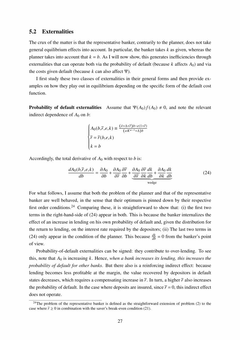
5.2 Externalities

The crux of the matter is that the representative banker, contrarily to the planner, does not takegeneral equilibrium effects into account. In particular, the banker takes k as given, whereas theplanner takes into account that k = b. As I will now show, this generates inefficiencies throughexternalities that can operate both via the probability of default (because k affects A0) and viathe costs given default (because k can also affect Ψ).

I first study these two classes of externalities in their general forms and then provide ex-amples on how they play out in equilibrium depending on the specific form of the default costfunction.

Probability of default externalities Assume that Ψ(A0) f (A0) , 0, and note the relevantindirect dependence of A0 on b:

A0(b,r ,e,k) ≡ (δ+∆+r)b−e(1+r)(αKα−1+∆)b

r = r (b,e,k)

k = b

Accordingly, the total derivative of A0 with respect to b is:

dA0(b,r ,e,k)db

=∂A0

∂b+∂A0

∂r∂r∂b+∂A0

∂r∂r∂k

dkdb+∂A0

∂kdkdb︸ ︷︷ ︸

wedge

(24)

For what follows, I assume that both the problem of the planner and that of the representativebanker are well behaved, in the sense that their optimum is pinned down by their respectivefirst order conditions.24 Comparing these, it is straightforward to show that: (i) the first twoterms in the right-hand-side of (24) appear in both. This is because the banker internalizes theeffect of an increase in lending on his own probability of default and, given the distribution forthe return to lending, on the interest rate required by the depositors; (ii) The last two terms in(24) only appear in the condition of the planner. This because dk

db = 0 from the banker’s pointof view.

Probability-of-default externalities can be signed: they contribute to over-lending. To seethis, note that A0 is increasing k. Hence, when a bank increases its lending, this increases the

probability of default for other banks. But there also is a reinforcing indirect effect: becauselending becomes less profitable at the margin, the value recovered by depositors in defaultstates decreases, which requires a compensating increase in r . In turn, a higher r also increasesthe probability of default. In the case where deposits are insured, since r = 0, this indirect effectdoes not operate.

24The problem of the representative banker is defined as the straightforward extension of problem (2) to thecase where r ≥ 0 in combination with the saver’s break-even condition (21).

27

Cost given default externalities Following the same logic as above, consider the generalcost function Ψ

(A,r ,b,e,k

)and note the relevant indirect dependence:

r = r (b,e,k)

B = b

The total derivative is:

dΨ(A,b,r ,e,k

)db

=∂Ψ

∂b+∂Ψ

∂r∂r∂b+∂Ψ

∂r∂r∂k

dkdb+∂Ψ

∂kdkdb︸ ︷︷ ︸

wedge

(25)

The last two terms identify another wedge in the banker’s first order condition. The last termis the direct effect, and the penultimate the indirect effect through the interest rate required bydepositors. Again, only the direct effect would operate if deposits were insured.

Contrarily to above, cost given default externalities can not always be signed, as they dependon the specific form for Ψ. I illustrate this in what follows.

5.3 Examples

Specification 1: Financial distress In the case where r ≥ 0, the cost function used in themain analysis generalizes to:

Ψ1 ≡ γ[(b− e)(1+ r (b,e,k))− b(1+ r (A,k))

]+ .First, by construction, we have Ψ1(A0) = 0. Hence, even though an increase in lending doesincrease the probability of default of other banks, this is not a source of inefficiency.25 Second,from equation (25), lending expansion by a bank increases the costs given default of otherbanks if

∂Ψ1

∂k+∂Ψ1

∂r∂r∂k≥ 0.

And this is the case: an increase in k decreases the marginal return to lending, which, ceterisparibus, increases default costs. Both directly (the first term is positive) and indirectly throughan increase in the required interest rate on deposits (the second term is positive too). Hence,we get overlending (and therefore overinvestment) in the competitive equilibrium, even in theabsence of government guarantees.26

25If the support for A is not continuous, then even though Ψ(A0) = 0, probability-of-default externalities canlead to inefficiency. For instance, assuming A ∈ AL ,AH , with AL < AH , it is easy to construct an example wherebanks default in state AL in the competitive equilibrium, but not in the socially optimal allocation.

26Even though the mechanism at their source is different, this case of the model shares the investment efficiencyproperties of many fire-sales model (see, e.g. Lorenzoni (2008) and Jeanne and Korinek (2013)). That is, under-investment with respect to first best (i.e. the efficient allocation if bank capital wasn’t scarce), but overinvestmentwith respect to second best (interpreted as k∗

t+1).

28

There are several possible interpretation for Ψ1. As mentioned in Section 4, one can thinkof deadweight losses emanating from the bank resolution process.27 Arguably, this processwill be longer and costlier when financial distress is high. Alternatively, in the presence ofgovernment guarantees, one can think of the default costs as a proxy for the deadweight lossesof taxation associated to bailouts (see, e.g., Acharya et al. (2010) and Bianchi (2013)).

In specification Ψ1, the costs are linear in financial distress and, therefore, in the amountneeded for the bailout (this is the assumption in Acharya et al., 2010). Hence, the externalityis not one where financial distress at a bank increases, in itself, the likelihood or the extent ofother banks’ financial distress. It is therefore quite different from a fire sale externality. Thatsaid, making γ an increasing function of aggregate financial distress would be an easy way toadd a fire-sale flavor to the model, and to magnify the externality.

Finally, note that specification Ψ1 is consistent with Townsend’s baseline assumptions inhis seminal paper that establishes the optimality of standard debt contracts in a costly-state-verification environment (see Proposition 3.1 in Townsend (1979)).28 Townsend (1979) stressesthe analytical convenience of such a specification, but he also considers fixed verification costs.This is the case I now turn to.

Specification 2: Balance sheet size The problem studied by Townsend (1979) is of fixedsize. In the present context, the natural interpretation of a fixed verification cost is one that isproportional to the size of the bank. Formally, conditional on default, this gives:

Ψ2 ≡ γb.

In this case, there is no cost-given-default externality. Formally, since Ψ2 does not depend onr or k , the wedge in expression (25) is nil. However, probability-of-default externalities dooperate (A0 still depends on r and k).

This implies that under specification Ψ2, as is the case under Ψ1, the competitive equilib-rium exhibits overlending, even in the absence of government guarantees. I have chosen to usespecification Ψ1 for the main analysis because I find it intuitively more appealing, and becauseof its analytical convenience (having Ψ(A0) = 0 makes the problem particularly well behaved).Arguably, the deadweight losses associated with a bank’s insolvency are likely to be increas-ing both in the extent of financial distress and on the size of the bank (Acharya et al. (2010)).One could therefore argue in favor of a cost function which would mix these two ingredients.

27Bankruptcies often involve deadweight losses (Townsend (1979)). In the case of financial institutions, lossescan be large (James (1991)), and banking crises are typically followed by long and painful recessions (Reinhartand Rogoff (2009)) involving permanent output losses (Cerra and Saxena (2008)).

28Specifically, the equivalence is as follows. In Townsend (1979) and following his own notation, the assump-tion for Proposition 3.1 is that verification costs are increasing and convex in C− g(y2), where C is the repaymentin absence of default (i.e. when no verification occurs) and g(y2) is the repayment in the case of default (i.e. whenverification occurs). Townsend then goes on with the example where verification costs are simply λ(C − g(y2)),where λ is a positive constant, which is thus equivalent to Ψ1.

29

However, as I have explained in the previous section, using specification Ψ2 in the numericalanalysis does not substantially affect the results. Using such an hybrid cost function is thereforeunlikely to affect them either.

Specification 3: Value of distressed assets Finally, I consider the case where default costsare proportional to the value of distressed assets. That is, conditional on default:

Ψ3 ≡ γbr (A,k)

Since Ψ3 depends on k (through r), the cost-given-default externality operates. The term thatbanks do not internalize is:

∂Ψ3

∂kdkdb= γbαA (α−1) kα−2 < 0.

It is negative, which means that bankers do not internalize that their credit expansion decreases

the default cost for other banks because it increases the losses they make on their loans. SinceΨ3(A0) > 0, the probability-of-default externality also contributes to the wedge, but with theopposite sign. Hence, the net effect cannot be signed. If f (A0) is small enough, the net effectis negative, and we get underinvestment in the competitive equilibrium (it is easy to generatean example with a discrete probability distribution function for At).

For non financial firms, specification Ψ3 has the natural interpretation that the deadweightlosses increase in the value of the firm’s capital stock (think of the additional wear and tearof machines that should be reallocated, or as fruit that rots on the shelves during a bankruptcyprocedure). In the context of financial assets, the interpretation is less clear, and the sign of theexternality is counter-intuitive. This result can, however, be related to the result in Hennessy(2004) that debt overhang problems are worse when the value recovered by creditors in defaultis high. That financial frictions can lead to counter-intuitive externalities also relates to thework of Davila and Korinek (2017).

A specification equivalent to Ψ3 was used in Bernanke and Gertler (1989) and in manypapers of the financial accelerator literature that followed (e.g. Carlstrom and Fuerst (1997);Bernanke, Gertler and Gilchrist (1999)). My analysis sheds new light on the mechanismsby which the financial accelerator operates and on related normative considerations. Underspecification Ψ3, a decrease in an agent’s net worth generates, in equilibrium, an increase inthe deadweight losses for other banks, which (assuming there are no government guarantees)makes them reduce their lending. To the best of my knowledge, the role of probability-of-default and cost-given-default externalities in financial accelerator models, and in particularthat they pull aggregate lending in opposite directions, had not been discussed yet.

30

6 Discussion of the model’s key ingredients

A central result in this paper is that when aggregate bank capital increases, the banking sectorshould be allowed to expand but less than proportionally. Hence, the capital requirement shouldbe tightened.

This result is robust in the sense that it does not hinge on specific parameter values andis in fact due to very few ingredients. The first of these ingredients is diminishing return tophysical capital. This is perhaps the most standard assumption in macroeconomics, but is oftenabstracted from the literature on banking and financial regulation (notable exceptions includeMartinez-Miera and Suarez (2014), and Van den Heuvel (2008)).

The second ingredient, is that bank credit supply matters for physical capital accumulation.In the model, I assume that banks are the only source of funding for firms, but this is notnecessary to generate the result. What really matters is that aggregate bank lending affectsaggregate real investment at the margin. Even though this seems to be a reasonable startingpoint, this is often abstracted from the macroeconomic literature. It is, however, now at thecore of current policy debates and there is a fast growing literature on the subject that builds oncontributions such as Holmström and Tirole (1997) for instance.29

Third, and perhaps most importantly, capital requirements affect aggregate lending, whichneed not (always) be the case in reality. There is no consensus on the subject (see Repullo andSuarez (2013)). For instance, there is evidence that banks do hold buffers above the regulatorylevel (Gropp and Heider, 2010), but there is also evidence of the relevance of bank capital re-quirements on credit supply in general (Bernanke, Lown and Friedman (1991); Thakor (1996);Ivashina and Scharfstein (2010); Aiyar, Calomiris and Wieladek (2012)). There also is evi-dence that changes in capital requirements affect bank lending (Jimenez et al. (2014); Bahajand Malherbe (2016)).30 And indeed, what matters for my analysis is that the requirements areessentially constraining lending. That is, what matters is that the capital requirement stanceaffects their behavior, even if the requirement is not technically binding. The huge resistanceof banks (through lobbying for instance) to structural increases in capital adequacy ratios andthe strong evidence of “risk-weight optimization” and regulatory arbitrage by the banks op-erating under the Basel II regime (buying CDS on ABS from AIG was one typical way toexplicitly circumvent the regulation for instance, see Yorulmazer (2013)) all indicate that capi-tal requirements do constrain bank decisions (see also Begley, Purnanandam and Zheng (2014);Mariathasan and Merrouche (2014)). In the model, capital requirements are binding becausebanks do not fully internalize the social cost of lending. This is likely to be the case in real-ity. First, because deposits are insured in most advanced economies, and there is evidence thatit does distort banks’ cost of borrowing (Demirguc-Kunt and Detragiache (2002); Ioannidouand Penas (2010)). Second, because large banks benefit from implicit guarantees (Acharya,

29See Brunnermeier, Eisenbach and Sannikov (2013) for a survey of recent developments, and Suarez (2010)for an insightful discussion of the various modeling strategies.

30See also Kashyap, Tsomocos and Vardoulakis (2014).

31

Anginer and Warburton (2014); Gandhi and Lustig (2015); Kelly, Lustig and Van Nieuwer-burgh (2011); Laeven (2000); Noss and Sowerbutts (2012)). And, last but not least, becausefinancial frictions can generate pecuniary externalities. A number of recent papers have fo-cused on fire sales externalities and alike (see Davila and Korinek (2017) for a synthesis), butthe mechanism I highlight in this paper had been overlooked so far.

7 Conclusion

I have studied economies where banks do not fully internalize the social costs of lending. Ina competitive equilibrium, this translates into over-investment by firms. The regulator canrestore investment efficiency thanks to a time-varying capital requirement. A key of its featuresis that it is increasing in aggregate bank capital. A regulatory regime that overlooks such abank capital channel will unnecessarily magnify business and financial cycle fluctuations. Acalibration of the model suggests that the associated welfare losses are substantial. I thereforebelieve that studying the real-world determinants of aggregate bank capital accumulation is animportant avenue for future research.31

ReferencesAcharya, Viral V, and Matthew Richardson. 2009. “Causes of the financial crisis.” Critical Review,

21(2-3): 195–210.

Acharya, Viral V, Deniz Anginer, and A Joseph Warburton. 2014. “The end of market discipline?investor expectations of implicit state guarantees.” mimeo, NYU.

Acharya, Viral V, Irvind Gujral, Nirupama Kulkarni, and Hyun Song Shin. 2011. “Dividends andbank capital in the financial crisis of 2007-2009.” NBER Working Paper Series.

Acharya, Viral V, João AC Santos, Tanju Yorulmazer, et al. 2010. “Systemic risk and depositinsurance premiums.” Economic Policy Review, , (Aug): 89–99.

Admati, A.R., P.M. DeMarzo, M.F. Hellwig, and P. Pfleiderer. 2010. “Fallacies, Irrelevant Facts,and Myths in the Discussion of Capital Regulation: Why Bank Equity is Not Expensive.”

Adrian, Tobias, and Hyun Shin. 2010. “Liquidity and Leverage.” Journal of Financial Intermedia-tion, 19(3).

Aiyar, Shekhar, Charles W Calomiris, and Tomasz Wieladek. 2012. “Does macro-pru leak? Evi-dence from a UK policy experiment.” NBER Working Paper Series.

Allen, Franklin, and Elena Carletti. 2013. “Deposits and bank capital structure.”

31Our current understanding of bank dynamic capital structure decisions is at best incomplete, especially ingeneral equilibrium (see the discussions in Allen and Carletti (2013), and Repullo and Suarez (2013) for instance,and Rampini and Viswanathan (2014), He and Krishnamurthy (2011), and Coimbra and Rey (2017) for recentadvances).

32

Bahaj, Saleem, and Frédéric Malherbe. 2016. “A positive analysis of bank behaviour under capitalrequirements.”

BCBS. 1988. “International convergence of capital measurement and capital standards (Basel I).”Basel Committee on Banking Supervision.

BCBS. 2004. “Basel II: International Convergence of Capital Measurement and Capital Stan-dards: A Revised Framework.” Basel Committee on Banking Supervision.

BCBS. 2010. “Basel III: A global regulatory framework for more resilient banks and bankingsystems.” Basel Committee on Banking Supervision.

Begenau, Juliane. 2015. “Capital Requirement, Risk Choice, and Liquidity Provision in a BusinessCycle Model.” mimeo, HBS.

Begley, Taylor, Amiyatosh Purnanandam, and Kuncheng Zheng. 2014. “The Strategic Under-Reporting of Bank Risk.” mimeo, London Business School.

Bernanke, Ben, and Mark Gertler. 1989. “Agency Costs, Net Worth, and Business Fluctuations.”American Economic Review, 79(1): 14–31.

Bernanke, Ben, Mark Gertler, and Simon Gilchrist. 1999. “The financial accelerator in a quanti-tative business cycle framework,.” (Elsevier).

Bernanke, Ben S, Cara S Lown, and Benjamin M Friedman. 1991. “The credit crunch.” Brookingspapers on economic activity, 205–247.

Bianchi, J. 2011. “Overborrowing and systemic externalities in the business cycle.” American Eco-nomic Review, 101(7): 3400–3426.

Bianchi, Javier. 2013. “Efficient bailouts?” mimeo, University of Wisconsin.

Boissay, Frederic, Fabrice Collard, and Frank Smets. 2013. “Booms and Banking Crises.” mimeo,ECB.

Borio, C., and M. Drehmann. 2009. “Assessing the risk of banking crises–revisited.” BIS QuarterlyReview, 29–46.

Brunnermeier, Markus K., Thomas Eisenbach, and Yuliy Sannikov. 2013. “Macroeconomics withFinancial Frictions: A Survey.” Advances in Economics and Econometrics, Tenth World Congressof the Econometric Society. New York:Cambridge University Press.

Carlstrom, Charles T, and Timothy S Fuerst. 1997. “Agency costs, net worth, and business fluctu-ations: A computable general equilibrium analysis.” The American Economic Review, 893–910.

Catarineu-Rabell, Eva, Patricia Jackson, and Dimitrios P Tsomocos. 2005. “Procyclicality and thenew Basel Accord-banks’ choice of loan rating system.” Economic Theory, 26(3): 537–557.

Cerra, Valerie, and Sweta Chaman Saxena. 2008. “Growth dynamics: the myth of economic re-covery.” The American Economic Review, 98(1): 439–457.

Coeurdacier, Nicolas, Hélène Rey, and Pablo Winant. 2011. “The Risky Steady State.” The Amer-ican Economic Review, 101(3): 398–401.

Coimbra, Nuno, and Hélene Rey. 2017. “Financial Cycles with Heterogeneous Intermediaries.”NBER Working Paper 23245.

33

Davila, Eduardo, and Anton Korinek. 2017. “Pecuniary Externalities in Economies with FinancialFrictions.” Review of Economic Studies.

Demirguc-Kunt, Asli, and Enrica Detragiache. 2002. “Does deposit insurance increase bankingsystem stability? An empirical investigation.” Journal of Monetary Economics, 49(7): 1373–1406.

Dewatripont, Mathias, and Jean Tirole. 2012. “Macroeconomic shocks and banking regulation.”Journal of Money, Credit and Banking, 44(s2): 237–254.

Farhi, Emmanuel, and Iván Werning. 2013. “A theory of macroprudential policies in the presenceof nominal rigidities.” NBER Working Paper Series.

Floyd, Eric, Nan Li, and Douglas J Skinner. 2015. “Payout policy through the financial crisis:The growth of repurchases and the resilience of dividends.” Journal of Financial Economics,118(2): 299–316.

Gandhi, Priyank, and Hanno Lustig. 2015. “Size anomalies in US bank stock returns.” The Journalof Finance, 70(2): 733–768.

Gersbach, Hans, and Jean-Charles Rochet. 2012. “Aggregate investment externalities and macro-prudential regulation.” Journal of Money, Credit and Banking, 44(s2): 73–109.

Gertler, M., and N. Kiyotaki. 2010. “Financial intermediation and credit policy in business cycleanalysis.” Handbook of Monetary Economics, 3: 547.

Goodhart, Charles AE, Anil K Kashyap, Dimitrios P Tsomocos, and Alexandros P Vardoulakis.2012. “Financial regulation in general equilibrium.” National Bureau of Economic Research.

Gromb, Denis, and Dimitri Vayanos. 2002. “Equilibrium and welfare in markets with financiallyconstrained arbitrageurs.” Journal of Financial Economics, 66(2-3): 361–407.

Gropp, Reint, and Florian Heider. 2010. “The Determinants of Bank Capital Structure.” Reviewof Finance, 14(4): 587–622.

Hanson, S., A. Kashyap, and J. Stein. 2011. “A macroprudential approach to financial regulation.”Journal of Economic Perspectives, 25(1): 3–28.

Harris, Milt, Christian Opp, and Marcus Opp. 2015. “Macroprudential bank capital regulationin a competitive financial system.” mimeo, Berkeley.

Hennessy, Christopher A. 2004. “Tobin’s Q, debt overhang, and investment.” The Journal of Fi-nance, 59(4): 1717–1742.

He, Zhiguo, and Arvind Krishnamurthy. 2011. “A model of capital and crises.” The Review ofEconomic Studies.

Holmström, Bengt, and Jean Tirole. 1997. “Financial Intermediation, Loanable Funds, and theReal Sector.” The Quarterly Journal of Economics, 112(3): 663–91.

Ioannidou, Vasso P, and María Fabiana Penas. 2010. “Deposit insurance and bank risk-taking:Evidence from internal loan ratings.” Journal of Financial Intermediation, 19(1): 95–115.

Ivashina, Victoria, and David Scharfstein. 2010. “Bank lending during the financial crisis of 2008.”Journal of Financial economics, 97(3): 319–338.

34

James, Christopher. 1991. “The losses realized in bank failures.” The Journal of Finance,46(4): 1223–1242.

Jeanne, Olivier, and Anton Korinek. 2010. “Managing credit booms and busts: A Pigouvian taxa-tion approach.” mimeo.

Jeanne, Olivier, and Anton Korinek. 2013. “Macroprudential regulation versus mopping up afterthe crash.” NBER Working Paper Series.

Jimenez, Gabriel, Seven Ongena, Jesus Saurina, and Jose-Luis Peydro. 2014. “MacroprudentialPolicy, Countercyclical Bank Capital Buffers and Credit Supply: Evidence from the SpanishDynamic Provisioning Experiments.” Mimeo, UPF.

Jordà, Òscar, Moritz Schularick, and Alan M Taylor. 2013. “When credit bites back.” Journal ofMoney, Credit and Banking, 45(s2): 3–28.

Kareken, J.H., and N. Wallace. 1978. “Deposit insurance and bank regulation: A partial-equilibrium exposition.” Journal of Business, 413–438.

Kashyap, A.K., and J.C. Stein. 2004. “Cyclical implications of the Basel II capital standards.”Economic Perspectives - Federal Reserve Bank of Chicago, 28(1): 18–33.

Kashyap, Anil K, Dimitrios P Tsomocos, and Alexandros P Vardoulakis. 2014. “How does macro-prudential regulation change bank credit supply?” National Bureau of Economic Research.

Kelly, Bryan T, Hanno Lustig, and Stijn Van Nieuwerburgh. 2011. “Too-systemic-to-fail: Whatoption markets imply about sector-wide government guarantees.” National Bureau of EconomicResearch.

Korinek, Anton, and Alp Simsek. 2016. “Liquidity trap and excessive leverage.” The AmericanEconomic Review, 106(3): 699–738.

Krishnamurthy, Arvind. 2003. “Collateral constraints and the amplification mechanism.” Journalof Economic Theory, 111(2): 277–292.

Laeven, Luc. 2000. “Banking risks around the world: The implicit safety net subsidy approach.”World Bank Policy Research Working Paper, , (2473).

Laeven, Luc, and Fabian Valencia. 2012. “Systemic banking crises database: An update.”

Lorenzoni, Guido. 2008. “Inefficient credit booms.” Review of Economic Studies, 75(3): 809–833.

Lucas, Robert. 2003. “Macroeconomic priorities.” The American Economic Review, 93(1): 1.

Mariathasan, Mike, and Ouarda Merrouche. 2014. “The manipulation of basel risk-weights.”Journal of Financial Intermediation, 23(3): 300–321.

Martinez-Miera, D., and J. Suarez. 2014. “A Macroeconomic Model of Endogenous Systemic RiskTaking.” mimeo, CEMFI.

Morrison, Alan D, and Lucy White. 2005. “Crises and capital requirements in banking.” AmericanEconomic Review, 1548–1572.

Noss, Joseph, and Rhiannon Sowerbutts. 2012. “The implicit subsidy of banks.” Bank of EnglandFinancial Stability Paper, 15.

35

Perotti, E.C., and J. Suarez. 2002. “Last bank standing: what do I gain if you fail?” Europeaneconomic review, 46(9): 1599–1622.

Rampini, Adriano A, and S Viswanathan. 2014. “Financial Intermediary Capital.” Mimeo, DukeUniversity.

Reinhart, Carmen M, and Kenneth Rogoff. 2009. This time is different: Eight centuries of financialfolly. Princeton University Press.

Repullo, Rafael. 2013. “Cyclical adjustment of capital requirements: A simple framework.” Jour-nal of Financial Intermediation, 22(4): 608–626.

Repullo, Rafael, and Javier Suarez. 2013. “The procyclical effects of bank capital regulation.”Review of Financial Studies, 26(2): 452–490.

Repullo, Rafael, Jesús Saurina, and Carlos Trucharte. 2010. “Mitigating the Pro-cyclicality ofBasel II.” Economic Policy, 25(64): 659–702.

Rognlie, Matthew, Andrei Shleifer, and Alp Simsek. 2014. “Investment Hangover and the GreatRecession.” National Bureau of Economic Research.

Shleifer, Andrei, and Robert W. Vishny. 1997. “The Limits of Arbitrage.” Journal of Finance,52(1): 35–55.

Stein, Jeremy. 2012. “Monetary policy as financial-stability regulation.” Quarterly Journal of Eco-nomics, 127: 57–95.

Suarez, Javier. 2010. “Discussion of: Procyclicality of capital requirements in a general equilib-rium model of liquidity dependence.” International Journal of Central Banking, forthcoming.

Thakor, Anjan V. 1996. “Capital requirements, monetary policy, and aggregate bank lending:theory and empirical evidence.” The Journal of Finance, 51(1): 279–324.

Townsend, Robert M. 1979. “Optimal contracts and competitive markets with costly state verifi-cation.” Journal of Economic theory, 21(2): 265–293.

Van den Heuvel, Skander J. 2008. “The welfare cost of bank capital requirements.” Journal ofMonetary Economics, 55(2): 298–320.

Yorulmazer, Tanju. 2013. “Has Financial Innovation Made the World Riskier? CDS, RegulatoryArbitrage and Systemic Risk.” Mimeo.

Appendix A: Proofs

Proposition. 1. At all dates, the competitive equilibrium capital stock is inefficiently high. That

is: kCEt+1 > k∗t+1,∀t.

Proof. The representative banker maximizes Et[[btrt+1+ et]+

]− et with respect to et ,bt ≥ 0 .

The respective first order conditions are:

∫ ∞ρt+1

f t (rt+1)drt+1 ≤ 1∫ ∞ρt+1

rt+1 f t (rt+1)drt+1 ≤ 0 ,

36

where f t is the probability distribution function of rt+1 conditional to date-t information, andρt+1 ≡ −

etbt

is the solvency threshold. That is, this is the value for rt+1 below which the bankdefaults..

Efficiency requires Et[rt+1] ≥ 0. Given the banker’s first order condition, Et[rt+1] > 0 cannotbe true in equilibrium. The only case where the competitive equilibrium could be efficient iswhen efficiency requires Et[rt+1] = 0. Assume that this is the case and consider the first orderconditions.

If Et[rt+1] = 0, the only way for both conditions to be satisfied is for the bank never todefault. If this is the case, the bank is locally indifferent between financing the loans withdeposits or equity. Now, imagine that the bank substitutes deposits for equity (keeping lendingconstant) up to the point where it fails if a low At realizes. From this point on, decreasing equityfurther increases expected profits (for each unit of equity withdrawn today, less than a unit isrepaid to depositors tomorrow in expectation). Hence, the bank defaults with strictly positiveprobability in equilibrium and, given the first order conditions, Et[rt+1] = 0 cannot be satisfiedin equilibrium.32

Proposition. 2. The regulator can ensure investment efficiency, at all t, with the following

capital requirement

x∗t =ηtwt

k∗t+1. (26)

Proof. Given that aggregate bank capital is assumed to be scarce (i.e. ηtwt < k∗t+1) and thatefficiency requires Et[rt+1] ≥ 0, bankers find it profitable to invest all their wealth in equity.Assume the representative bank defaults in equilibrium. Then, following the same logic asin the proof of Proposition 1, the banker always prefer to finance loans with deposits at themargin. Hence the capital requirement must be binding, and k∗t+1 = et/x∗t in equilibrium. If therepresentative bank does not default in the constrained equilibrium, a similar logic applies butthe optimal capital requirement is not unique.

Proposition. 3. ∀t, κt < 1. Hence the optimal capital requirement is increasing in aggregate

bank capital.

Proof. Since b∗t = k∗t+1, I need to show thatdk∗

t+1k∗t+1/ det

et< 1. Ignoring subscripts and superscripts,

I can rewrite economic surplus:

S = ¯E[A]kα − (δ+ (1−E[A])∆)) k −γ∫ A0

0

((δ+ (1− A)∆)) k −αAkα − e

)f (A) dA,

whereA0 ≡

(δ+∆) k − eαkα +∆k

.

32See the working paper version for a proof of equilibrium existence (anonymized reference).

37

From the first order condition associated with the maximization of S with respect to k, I candefine a function G(k,e) = 0

G(k,e) ≡ αE[A]kα−1− (δ+ (1−E[A])∆))−γ∫ A0

0

((δ+ (1− A)∆))−α2 Akα−1

)f (A) dA = 0.

Applying the implicit function theorem, I need to show that(∂G∂e

)/(− ∂G∂k

)< k

e . That is,

γ(−∂A0∂e

)f (A0)Ω

α(1−α)E[A]kα−2+γ∫ A0

0(α2 (1−α) Akα−2) f (A) dA+γ

(∂A0∂k

)f (A0)Ω

<ke, (27)

where

Ω ≡((δ+ (1− A0)∆))−α2 A0kα−1

).

We have:

∂A0∂e =

−1αkα+∆k

∂A0∂k =

(δ+∆)(αkα+∆k)−(α2kα−1+∆)((δ+∆)k−e)(αkα+∆k)2 .

By the definition of A0, we have that (δ+ (1− A0)∆)) > αA0kα−1. Hence, Ω > 0 and thenumerator in (27) is positive. Given that the first two terms of the denominator are also positive,it is sufficient to show that:

−∂A0

∂e/∂A0

∂k<

ke. (28)

Noting that ∂A0∂k > 0, condition (28) becomes:

eαkα +∆k

<(δ+∆) (αkα +∆k)−

(α2kα−1+∆

)((δ+∆) k − e)

(αkα +∆k)2 k,

which boils down to:

k(α2kα−1+∆

)((δ+∆) k − e) < ((δ+∆) k − e)

(αkα +∆k

),

which holds since ((δ+∆) k − e) > 0 (otherwise A0 = AL and banks do not default in equilib-rium), and α < 1.

Proposition. 4. Assume default is costless (γ = 0 and ∆ = 0). The bank capital channel domi-

nates the default rate channel at any positive lag. In the period where the shock occurs, this is

true if the shock is not too persistent. Formally, following a date-1 positive productivity shock,

E1[xt>1] > 0, and x1 > 0⇔ ρ < 1−α.

Proof. The proof follows exactly the same logic as the example in the text. The only differenceis that one needs to take expectations to account for the realizations of ε t>1.

38

Appendix B: Alternative default cost function

Figure 5 and Table 4 present results under the alternative bank default cost function (specifica-tion Ψt+1 = btγp). The value for the cost parameter is chosen so that the expected costs givendefault are comparable to those under the baseline calibration. That is γp = 0.02, which yieldsan expected deadweight loss (conditional on default) of 5.88% of steady state GDP. As we cansee, both the impulse responses and the loss distributions are very similar to what I get with mybaseline specification (see Figures 1 and 2 and Table 3). Finally, note that the welfare loss isessentially unchanged (it remains around 0.04% of steady state consumption).

Figure 5: Bank default costs proportional to balance sheet

This figure presents the results under the assumption that Ψt+1 = 0.02bt if the bank defaults, and 0 otherwise. Theleft panel shows the path for the optimal capital requirement x∗t , and the alternative policy, starting from steadystate and following a 1% decrease in the loan default rate. The right panel shows the path for the optimal capitalrequirement after a triple negative shock for two different values of γp.

Table 4: Loss frequenciesγ = 2 γ = 4 γprop = 0.02

Freq. of large losses 16.4% 15.9% 16.0%in good time 7.1% 6.9% 7%

in bad times 29.1% 26.9% 28%Probability of default 0.13% 0.08% 0.11%

This table compares simulated moments between the baseline specification for the default cost function (withγ = 2 and γ = 4) and the alternative specification Ψt+1 = 0.02bt . Other parameters are at their baseline value(Table 1). All simulations start at steady state, and follow the exact same arbitrary sequence of 10,000 randomshocks. Good times (bad times) are defined as periods where the loan default rate is at list one standard deviationbelow (above) the sample mean. Large losses correspond to losses larger than 10% of initial bank capital.

39

Appendix C: Comparing policies

Table 5: Further simulation results (baseline calibration)x∗t x

′

t

Lending volatility std (bt ) 1.98 2.19Probability of default mean (Prt (vt+1 < 0)) 0.13% ' 0Freq. of large losses ROE < −10% 16.4% 16.0%

in good time 7.1% 12.1%in bad times 29.1% 11.8%

Dividend / recap (et − et ) /et 0 1.6%in good time 0 7.1%in bad times 0 −3.4%

Welfare loss mean(S∗t − S

′

t

)/Sss - 0.04%

This table compares simulated moments under the optimal capital requirement (x∗) and the alternative policy(x′

). Both simulations use baseline calibration parameters (Table 1), start at steady state, and follow the exactsame arbitrary sequence of 10,000 random shocks. Good times (bad times) are defined as periods where the loandefault rate is at list one standard deviation below (above) the sample mean. ROE is defined as

(v+t+1/et

)− 1.

Variable et denotes the pre-dividend (and pre-recapitalization) level of aggregate bank equity at the end of date t.Finally, S∗t and S

′

t are the realized surplus under the respective policies.

Appendix D: Summary of intraperiod time-line

1. At is realized and publicly observed, firms competitively hire workers.

2. Production takes place and is allocated: wages are paid, solvent firms repay their loan,insolvent firms transfer their residual value to the banks.

3. If solvent, banks repay depositors. If insolvent, banks default and the associated costsare incurred by the depositors. The regulator compensates them for their losses and taxessavers to break even.

4. Young agents learn whether they have banking ability.

5. Young bankers make their investment portfolio decision (storage and/or investment intheir bank’s equity).

6. Banks borrow from savers and lend to firms, which invest in physical capital. Agents putthe remainder of their savings in the storage technology.

7. The old generation consumes and leaves the economy.

40