opencv 2 computer vision application programming cookbook · opencv 2 computer vision application...

OpenCV 2 Computer Vision Application Programming Cookbook

Robert Laganière

Chapter No.5

"Transforming Images with Morphological

Operations"

In this package, you will find: A Biography of the author of the book

A preview chapter from the book, Chapter NO.5 "Transforming Images with

Morphological Operations"

A synopsis of the book’s content

Information on where to buy this book

About the Author Robert Laganière is a professor at the University of Ottawa, Canada. He received his

Ph.D. degree from INRS-Telecommunications in Montreal in 1996. Dr. Laganière is a

researcher in computer vision with an interest in video analysis, intelligent visual

surveillance, and imagebased modeling. He is a co-founding member of the VIVA

research lab. He is also a Chief Scientist at iWatchLife.com, a company offering a cloud-

based solution for remote monitoring. Dr. Laganière is the co-author of Object-oriented

Software Engineering published by McGraw Hill in 2001.

Visit the author's website at http://www.laganiere.name.

I wish to thank all my students at the VIVA lab. I learn so much from

them. I am also grateful to my beloved Marie-Claude, Camille, and

Emma for their continuous support.

For More Information: www.PacktPub.com/opencv-2-computer-vision-application-

programming-cookbook/book

http://www.packtpub.com/opencv-2-computer-vision-application-programming-cookbook/book

OpenCV 2 Computer Vision Application Programming Cookbook In today's digital world, images and videos are everywhere, and with the advent of

powerful and affordable computing devices, it has never been easier to create

sophisticated imaging applications. Plentiful software tools and libraries manipulating

images and videos are offered, but for anyone who wishes to develop his/her own

applications, the OpenCV library is the tool to use.

OpenCV (Open Source Computer Vision) is an open source library containing more than

500 optimized algorithms for image and video analysis. Since its introduction in 1999, it

has been largely adopted as the primary development tool by the community of

researchers and developers in computer vision. OpenCV was originally developed at Intel

by a team led by Gary Bradski as an initiative to advance research in vision and promote

the development of rich, vision-based CPU-intensive applications. After a series of beta

releases, version 1.0 was launched in 2006. A second major release occurred in 2009 with

the launch of OpenCV 2 that proposed important changes, especially the new C++

interface which we use in this book. At the time of writing, the latest release is 2.2

(December 2010).

This book covers many of the library's features and shows how to use them to accomplish

specific tasks. Our objective is not to provide a complete and detailed coverage of every

option offered by the OpenCV functions and classes, but rather to give you the elements

you need to build your applications from the ground up. In this book we also explore

fundamental concepts in image analysis and describe some of the important algorithms in

computer vision.

This book is an opportunity for you to get introduced to the world of image and video

analysis. But this is just the beginning. The good news is that OpenCV continues to

evolve and expand. Just consult the OpenCV online documentation to stay updated about

what the library can do for you:

http://opencv.willowgarage.com/wiki/

What This Book Covers Chapter 1, Playing with Images, introduces the OpenCV library and shows you how to

run simple applications using the MS Visual C++ and Qt development environments.

Chapter 2, Manipulating the Pixels, explains how an image can be read. It describes

different methods for scanning an image in order to perform an operation on each of its

pixels. You will also learn how to define region of interest inside an image.




Chapter 3, Processing Images with Classes, consists of recipes which present various

object oriented design patterns that can help you to build better computer

vision applications.

Chapter 4, Counting the Pixels with Histograms, shows you how to compute image

histograms and how they can be used to modify an image. Different applications based

on histograms are presented that achieve image segmentation, object detection, and

image retrieval.

Chapter 5, Transforming Images with Morphological Operations, explores the concept of

mathematical morphology. It presents different operators and how they can be used to

detect edges, corners, and segments in images.

Chapter 6, Filtering the Images, teaches you the principle of frequency analysis and

image filtering. It shows how low-pass and high-pass filters can be applied to images. It

presents the two image derivative operators: the gradient and the Laplacian.

Chapter 7, Extracting Lines, Contours, and Components, focuses on the detection of

geometric image features. It explains how to extract contours, lines, and connected

components in an image.

Chapter 8, Detecting and Matching Interest Points, describes various feature point

detectors in images. It also explains how descriptors of interest points can be computed

and used to match points between images.

Chapter 9, Estimating Projective Relations in Images, analyzes the different relations

involved in image formation. It also explores the projective relations that exist between

two images of a same scene.

Chapter 10, Processing Video Sequences, provides a framework to read and write a video

sequence and to process its frames. It also shows you how it is possible to track feature

points from frame to frame, and how to extract the foreground objects moving in

front of a camera.




5Transforming Images

with Morphological Operations

In this chapter, we will cover:

Eroding and dilating images using morphological fi lters

Opening and closing images using morphological fi lters

Detecting edges and corners using morphological fi lters

Segmenting images using watersheds

Extracting foreground objects with the GrabCut algorithm

IntroductionMorphological fi ltering is a theory developed in the 1960s for the analysis and processing of discrete images. It defi nes a series of operators which transform an image by probing it with a predefi ned shape element. The way this shape element intersects the neighborhood of a pixel determines the result of the operation. This chapter presents the most important morphological operators. It also explores the problem of image segmentation using algorithms working on the image morphology.




Transforming Images with Morphological Operations

118

Eroding and dilating images using morphological fi lters

Erosion and dilation are the most fundamental morphological operators. Therefore, we will present them in this fi rst recipe.

The fundamental instrument in mathematical morphology is the structuring element . A structuring element is simply defi ned as a confi guration of pixels (a shape) on which an origin is defi ned (also called anchor point). Applying a morphological fi lter consists of probing each pixel of the image using this structuring element. When the origin of the structuring element is aligned with a given pixel, its intersection with the image defi nes a set of pixels on which a particular morphological operation is applied. In principle, the structuring element can be of any shape, but most often, a simple shape such as a square, circle, or diamond with the origin at the center is used (mainly for effi ciency reasons).

Getting ready As morphological fi lters usually work on binary images, we will use the binary image which was produced through thresholding in the fi rst recipe of the previous chapter. However, since in morphology, the convention is to have foreground objects represented by high (white) pixel values and background by low (black) pixel values, we have negated the image. In morphological terms, the following image is said to be the complement of the image that was produced in the previous chapter:




Chapter 5

119

How to do it... Erosion and dilation are implemented in OpenCV as simple functions which are cv::erode and cv::dilate. Their use is straightforward:

// Read input image cv::Mat image= cv::imread("binary.bmp");

// Erode the image cv::Mat eroded; // the destination image cv::erode(image,eroded,cv::Mat());

// Display the eroded image cv::namedWindow("Eroded Image");"); cv::imshow("Eroded Image",eroded);

// Dilate the image cv::Mat dilated; // the destination image cv::dilate(image,dilated,cv::Mat());

// Display the dilated image cv::namedWindow("Dilated Image"); cv::imshow("Dilated Image",dilated);

The two images produced by these function calls are seen in the following screenshot. Erosion is shown fi rst:





120

Followed by the dilation result:

How it works... As with all other morphological fi lters, the two fi lters of this recipe operate on the set of pixels (or neighborhood) around each pixel, as defi ned by the structuring element. Recall that when applied to a given pixel, the anchor point of the structuring element is aligned with this pixel location, and all pixels intersecting the structuring element are included in the current set. Erosion replaces the current pixel with the minimum pixel value found in the defi ned pixel set. Dilation is the complementary operator, and it replaces the current pixel with the maximum pixel value found in the defi ned pixel set. Since the input binary image contains only black (0) and white (255) pixels, each pixel is replaced by either a white or black pixel.

A good way to picture the effect of these two operators is to think in terms of background (black) and foreground (white) objects. With erosion, if the structuring element when placed at a given pixel location touches the background (that is, one of the pixels in the intersecting set is black), then this pixel will be sent to background. While in the case of dilation, if the structuring element on a background pixel touches a foreground object, then this pixel will be assigned a white value. This explains why in the eroded image, the size of the objects has been reduced. Observe how some of the very small objects (that can be considered as "noisy" background pixels) have also been completely eliminated. Similarly, the dilated objects are now larger and some of the "holes" inside of them have been fi lled.

By default, OpenCV uses a 3x3 square structuring element. This default structuring element is obtained when an empty matrix (that is cv::Mat()) is specifi ed as the third argument in the function call, as it was done in the preceding example. You can also specify a structuring element of the size (and shape) you want by providing a matrix in which the non-zero element defi nes the structuring element. In the following example, a 7x7 structuring element is applied:




Chapter 5

121

cv::Mat element(7,7,CV_8U,cv::Scalar(1)); cv::erode(image,eroded,element);

The effect is obviously much more destructive in this case as seen here:

Another way to obtain the same result is to repetitively apply the same structuring element on an image. The two functions have an optional parameter to specify the number of repetitions:

// Erode the image 3 times. cv::erode(image,eroded,cv::Mat(),cv::Point(-1,-1),3);

The origin argument cv::Point(-1,-1) means that the origin is at the center of the matrix (default), and it can be defi ned anywhere on the structuring element. The image obtained will be identical to the one we obtained with the 7x7 structuring element. Indeed, eroding an image twice is like eroding an image with a structuring element dilated with itself. This also applies to dilation.

Finally, since the notion of background/foreground is arbitrary, we can make the following observation (which is a fundamental property of the erosion/dilation operators). Eroding foreground objects with a structuring element can be seen as a dilation of the background part of the image. Or more formally:

The erosion of an image is equivalent to the complement of the dilation of the complement image.

The dilation of an image is equivalent to the complement of the erosion of the complement image.

There's more...It is important to note that even if we applied our morphological fi lters on binary images here, these can also be applied on gray-level images with the same defi nitions.





122

Also note that the OpenCV morphological functions support in-place processing. This means you can use the input image as the destination image. So you can write:

cv::erode(image,image,cv::Mat());

OpenCV creates the required temporary image for you for this to work properly.

See alsoThe next recipe which applies erosion and dilation fi lters in cascade to produce new operators.

The Detecting edges and corners using morphological fi lters for the application of morphological fi lters on gray-level images.

Opening and closing images using morphological fi lters

The previous recipe introduced the two fundamental morphological operators: dilation and erosion. From these, other operators can be defi ned. The next two recipes will present some of them. The opening and closing operators are presented in this recipe.

How to do it...In order to apply higher-level morphological fi lters, you need to use the cv::morphologyEx function with the appropriate function code. For example, the following call will apply the closing operator:

cv::Mat element5(5,5,CV_8U,cv::Scalar(1)); cv::Mat closed; cv::morphologyEx(image,closed,cv::MORPH_CLOSE,element5);

Note that here we use a 5x5 structuring element to make the effect of the fi lter more apparent. If we input the binary image of the preceding recipe, we obtain:




Chapter 5

123

Similarly, applying the morphological opening operator will result in the following image:

This one being obtained from the following code:

cv::Mat opened; cv::morphologyEx(image,opened,cv::MORPH_OPEN,element5);

How it works... The opening and closing fi lters are simply defi ned in terms of the basic erosion and dilation operations:

Closing is defi ned as the erosion of the dilation of an image.

Opening is defi ned as the dilation of the erosion of an image.





124

Consequently, one could compute the closing of an image using the following calls:

// dilate original image cv::dilate(image,result,cv::Mat()); // in-place erosion of the dilated image cv::erode(result,result,cv::Mat());

The opening would be obtained by inverting these two function calls.

While examining the result of the closing fi lter, it can be seen that the small holes of the white foreground objects have been fi lled. The fi lter also connects together several of the adjacent objects. Basically, any holes or gaps too small to completely contain the structuring element will be eliminated by the fi lter.

Reciprocally, the opening fi lter eliminated several of the small objects in the scene. All of the ones that were too small to contain the structuring element have been removed.

These fi lters are often used in object detection. The closing fi lter connects together objects erroneously fragmented into smaller pieces, while the opening fi lter removes the small blobs introduced by image noise. Therefore, it is advantageous to use them in sequence. If our test binary image is successively closed and opened, we obtain an image showing only the main objects in the scene, as shown below. You can also apply the opening fi lter before closing if you wish to prioritize noise fi ltering, but this can be at the price of eliminating some fragmented objects.

It should be noted that applying the same opening (and similarly the closing) operator on an image several times has no effect. Indeed, with the holes having been fi lled by the fi rst opening, an additional application of this same fi lter will not produce any other changes to the image. In mathematical terms, these operators are said to be idempotent.




Chapter 5

125

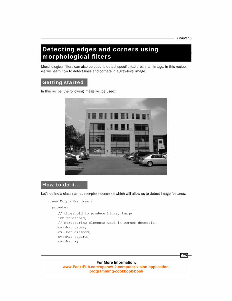
Detecting edges and corners using morphological fi lters

Morphological fi lters can also be used to detect specifi c features in an image. In this recipe, we will learn how to detect lines and corners in a gray-level image.

Getting startedIn this recipe, the following image will be used:

How to do it... Let's defi ne a class named MorphoFeatures which will allow us to detect image features:

class MorphoFeatures {

private:

// threshold to produce binary image int threshold; // structuring elements used in corner detection cv::Mat cross; cv::Mat diamond; cv::Mat square; cv::Mat x;





126

Detecting lines is quite easy using the appropriate fi lter of the cv::morphologyEx function:

cv::Mat getEdges(const cv::Mat &image) {

// Get the gradient image cv::Mat result; cv::morphologyEx(image,result, cv::MORPH_GRADIENT,cv::Mat());

// Apply threshold to obtain a binary image applyThreshold(result);

return result;}

The binary edge image is obtained through a simple private method of the class:

void applyThreshold(cv::Mat& result) {

// Apply threshold on result if (threshold>0) cv::threshold(result, result, threshold, 255, cv::THRESH_BINARY);}

Using this class in a main function, you then obtain the edge image as follows:

// Create the morphological features instanceMorphoFeatures morpho;morpho.setThreshold(40);

// Get the edgescv::Mat edges;edges= morpho.getEdges(image);




Chapter 5

127

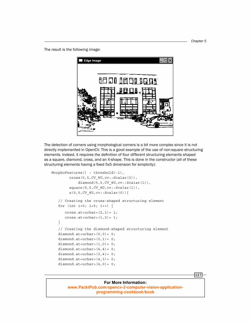
The result is the following image:

The detection of corners using morphological corners is a bit more complex since it is not directly implemented in OpenCV. This is a good example of the use of non-square structuring elements. Indeed, it requires the defi nition of four different structuring elements shaped as a square, diamond, cross, and an X-shape. This is done in the constructor (all of these structuring elements having a fi xed 5x5 dimension for simplicity):

MorphoFeatures() : threshold(-1), cross(5,5,CV_8U,cv::Scalar(0)), diamond(5,5,CV_8U,cv::Scalar(1)), square(5,5,CV_8U,cv::Scalar(1)), x(5,5,CV_8U,cv::Scalar(0)){

// Creating the cross-shaped structuring element for (int i=0; i<5; i++) {

cross.at<uchar>(2,i)= 1; cross.at<uchar>(i,2)= 1; }

// Creating the diamond-shaped structuring element diamond.at<uchar>(0,0)= 0; diamond.at<uchar>(0,1)= 0; diamond.at<uchar>(1,0)= 0; diamond.at<uchar>(4,4)= 0; diamond.at<uchar>(3,4)= 0; diamond.at<uchar>(4,3)= 0; diamond.at<uchar>(4,0)= 0;





128

diamond.at<uchar>(4,1)= 0; diamond.at<uchar>(3,0)= 0; diamond.at<uchar>(0,4)= 0; diamond.at<uchar>(0,3)= 0; diamond.at<uchar>(1,4)= 0;

// Creating the x-shaped structuring element for (int i=0; i<5; i++) {

x.at<uchar>(i,i)= 1; x.at<uchar>(4-i,i)= 1; } }

In the detection of corner features, all of these structuring elements are applied in cascade to obtain the resulting corner map:

cv::Mat getCorners(const cv::Mat &image) {

cv::Mat result;

// Dilate with a cross cv::dilate(image,result,cross);

// Erode with a diamond cv::erode(result,result,diamond);

cv::Mat result2; // Dilate with a X cv::dilate(image,result2,x);

// Erode with a square cv::erode(result2,result2,square);

// Corners are obtained by differencing // the two closed images cv::absdiff(result2,result,result);

// Apply threshold to obtain a binary image applyThreshold(result);

return result;}

In order to better visualize the result of the detection, the following method draws a circle on the image at each detected point on the binary map:

void drawOnImage(const cv::Mat& binary, cv::Mat& image) {

cv::Mat_<uchar>::const_iterator it= binary.begin<uchar>(); cv::Mat_<uchar>::const_iterator itend=




Chapter 5

129

binary.end<uchar>();

// for each pixel for (int i=0; it!= itend; ++it,++i) { if (!*it) cv::circle(image, cv::Point(i%image.step,i/image.step), 5,cv::Scalar(255,0,0)); }}

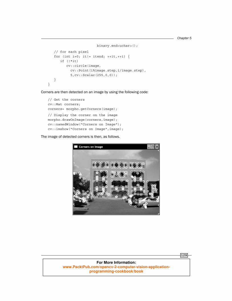
Corners are then detected on an image by using the following code:

// Get the cornerscv::Mat corners;corners= morpho.getCorners(image);

// Display the corner on the imagemorpho.drawOnImage(corners,image);cv::namedWindow("Corners on Image");cv::imshow("Corners on Image",image);

The image of detected corners is then, as follows.





130

How it works... A good way to help understand the effect of morphological operators on a gray-level image is to consider an image as a topological relief in which gray-levels correspond to elevation (or altitude). Under this perspective, bright regions correspond to mountains, while the darker areas form the valleys of the terrain. Also, since edges correspond to a rapid transition between darker and brighter pixels, these can be pictured as abrupt cliffs. If an erosion operator is applied on such a terrain, the net result will be to replace each pixel by the lowest value in a certain neighborhood, thus reducing its height. As a result, cliffs will be "eroded" as the valleys expand. Dilation has the exact opposite effect, that is, cliffs will gain terrain over the valleys. However, in both cases, the plateaux (that is, area of constant intensity) will remain relatively unchanged.

The above observations lead to a simple way of detecting the edges (or cliffs) of an image. This could be done by computing the difference between the dilated image and the eroded image. Since these two transformed images differ mostly at the edge locations, the image edges will be emphasized by the differentiation. This is exactly what the cv::morphologyEx function is doing when the cv::MORPH_GRADIENT argument is inputted. Obviously, the larger the structuring element is, the thicker the detected edges will be. This edge detection operator is also called the Beucher gradient (the next chapter will discuss the concept of image gradient in more detail). Note that similar results could also be obtained by simply subtracting the original image from the dilated one, or the eroded image from the original. The resulting edges would simply be thinner.

Corner detection is a bit more complex since it uses four different structuring elements. This operator is not implemented in OpenCV but we present it here to demonstrate how structuring elements of various shapes can be defi ned and combined. The idea is to close the image by dilating and eroding it with two different structuring elements. These elements are chosen such that they leave straight edges unchanged, but because of their respective effect, edges at corner points will be affected. Let's use the simple following image made of a single white square to better understand the effect of this asymmetrical closing operation:




Chapter 5

131

The fi rst square is the original image. When dilated with a cross-shaped structuring element, the square edges are expanded, except at the corner points where the cross shape does not hit the square. This is the result illustrated by the middle square. This dilated image is then eroded by a structuring element that, this time, has a diamond shape. This erosion brings back most edges at their original position, but pushes the corners even further since they were not dilated. The left square is then obtained, which, as it can be seen, has lost its sharp corners. The same procedure is repeated with an X-shaped and a square-shaped structuring element. These two elements are the rotated version of the previous ones and will consequently capture the corners at a 45-degree orientation. Finally, differencing the two results will extract the corner features.

See alsoThe article, Morphological gradients by J.-F. Rivest, P. Soille, S. Beucher, ISET's symposium on electronic imaging science and technology, SPIE, Feb. 1992, for more on morphological gradient.

The article A modifi ed regulated morphological corner detector by F.Y. Shih, C.-F. Chuang, V. Gaddipati, Pattern Recognition Letters , volume 26, issue 7, May 2005, for more information on morphological corner detection.

Segmenting images using watersheds The watershed transformation is a popular image processing algorithm that is used to quickly segment an image into homogenous regions. It relies on the idea that when the image is seen as a topological relief, homogeneous regions correspond to relatively fl at basins delimitated by steep edges. As a result of its simplicity, the original version of this algorithm tends to over-segment the image which produces multiple small regions. This is why OpenCV proposes a variant of this algorithm that uses a set of predefi ned markers which guide the defi nition of the image segments.

How to do it... The watershed segmentation is obtained through the use of the cv::watershed function. The input to this function is a 32-bit signed integer marker image in which each non-zero pixel represents a label. The idea is to mark some pixels of the image that are known to certainly belong to a given region. From this initial labeling, the watershed algorithm will determine the regions to which the other pixels belong. In this recipe, we will fi rst create the marker image as a gray-level image, and then convert it into an image of integers. We conveniently encapsulated this step into a WatershedSegmenter class :

class WatershedSegmenter {

private:





132

cv::Mat markers;

public:

void setMarkers(const cv::Mat& markerImage) {

// Convert to image of ints markerImage.convertTo(markers,CV_32S); }

cv::Mat process(const cv::Mat &image) {

// Apply watershed cv::watershed(image,markers);

return markers; }

The way these markers are obtained depends on the application. For example, some preprocessing steps might have resulted in the identifi cation of some pixels belonging to an object of interest. The watershed would then be used to delimitate the complete object from that initial detection. In this recipe, we will simply use the binary image used throughout this chapter in order to identify the animals of the corresponding original image (this is the image shown at the beginning of Chapter 4).

Therefore, from our binary image, we need to identify pixels that certainly belong to the foreground (the animals) and pixels that certainly belong to the background (mainly the grass). Here, we will mark foreground pixels with label 255 and background pixels with label 128 (this choice is totally arbitrary, any label number other than 255 would work). The other pixels, that is the ones for which the labeling is unknown, are assigned value 0. As it is now, the binary image includes too many white pixels belonging to various parts of the image. We will then severely erode this image in order to retain only pixels belonging to the important objects:

// Eliminate noise and smaller objects cv::Mat fg; cv::erode(binary,fg,cv::Mat(),cv::Point(-1,-1),6);




Chapter 5

133

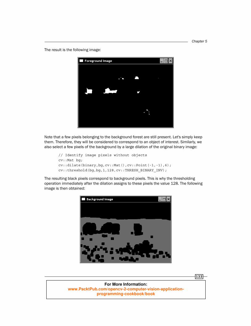
The result is the following image:

Note that a few pixels belonging to the background forest are still present. Let's simply keep them. Therefore, they will be considered to correspond to an object of interest. Similarly, we also select a few pixels of the background by a large dilation of the original binary image:

// Identify image pixels without objects cv::Mat bg; cv::dilate(binary,bg,cv::Mat(),cv::Point(-1,-1),6); cv::threshold(bg,bg,1,128,cv::THRESH_BINARY_INV);

The resulting black pixels correspond to background pixels. This is why the thresholding operation immediately after the dilation assigns to these pixels the value 128. The following image is then obtained:





134

These images are combined to form the marker image:

// Create markers image cv::Mat markers(binary.size(),CV_8U,cv::Scalar(0)); markers= fg+bg;

Note how we used the overloaded operator+ here in order to combine the images. This is the image that will be used as input to the watershed algorithm:

The segmentation is then obtained as follows:

// Create watershed segmentation object WatershedSegmenter segmenter;

// Set markers and process segmenter.setMarkers(markers); segmenter.process(image);

The marker image is then updated such that each zero pixel is assigned one of the input labels, while the pixels belonging to the found boundaries have value -1. The resulting image of labels is then:




Chapter 5

135

The boundary image is:

How it works... As we did in the preceding recipe, we will use the topological map analogy in the description of the watershed algorithm. In order to create a watershed segmentation, the idea is to progressively fl ood the image starting at level 0. As the level of "water" progressively increases (to levels 1, 2, 3, and so on), catchment basins are formed. The size of these basins also gradually increase and, consequently, the water of two different basins will eventually merge. When this happens, a watershed is created in order to keep the two basins separated. Once the level of water has reached its maximal level, the sets of these created basins and watersheds form the watershed segmentation.





136

As one can expect, the fl ooding process initially creates many small individual basins. When all of these are merged, many watershed lines are created which results in an over-segmented image. To overcome this problem, a modifi cation to this algorithm has been proposed in which the fl ooding process starts from a predefi ned set of marked pixels. The basins created from these markers are labeled in accordance with the values assigned to the initial marks. When two basins having the same label merge, no watersheds are created, thus preventing the over-segmentation.

This is what happens when the cv::watershed function is called. The input marker image is updated to produce the fi nal watershed segmentation. Users can input a marker image with any number of labels with pixels of unknown labeling left to value 0. The marker image has been chosen to be an image of a 32-bit signed integer in order to be able to defi ne more than 255 labels. It also allows the special value -1, to be assigned to pixels associated with a watershed. This is what is returned by the cv::watershed function. To facilitate the displaying of the result, we have introduced two special methods. The fi rst one returns an image of the labels (with watersheds at value 0). This is easily done through thresholding:

// Return result in the form of an image cv::Mat getSegmentation() {

cv::Mat tmp; // all segment with label higher than 255 // will be assigned value 255 markers.convertTo(tmp,CV_8U);

return tmp; }

Similarly, the second method returns an image in which the watershed lines are assigned value 0, and the rest of the image is at 255. This time, the cv::convertTo method is used to achieve this result:

// Return watershed in the form of an image cv::Mat getWatersheds() {

cv::Mat tmp; // Each pixel p is transformed into // 255p+255 before conversion markers.convertTo(tmp,CV_8U,255,255);

return tmp; }

The linear transformation that is applied before the conversion allows -1 pixels to be converted into 0 (since -1*255+255=0).

Pixels with a value greater than 255 are assigned the value 255. This is due to the saturation operation that is applied when signed integers are converted into unsigned chars.




Chapter 5

137

See alsoThe article The viscous watershed transform by C. Vachier, F. Meyer, Journal of Mathematical Imaging and Vision, volume 22, issue 2-3, May 2005, for more information on the watershed transform.

The next recipe which presents another image segmentation algorithm that can also segment an image into background and foreground objects.

Extracting foreground objects with the GrabCut algorithm

OpenCV proposes an implementation of another popular algorithm for image segmentation: the GrabCut algorithm . This algorithm is not based on mathematical morphology, but we present it here since it shows some similarities in its use with the watershed segmentation algorithm presented in the preceding recipe. GrabCut is computationally more expensive than watershed, but it generally produces a more accurate result. It is the best algorithm to use when one wants to extract a foreground object in a still image (for example, to cut and paste an object from one picture to another).

How to do it... The cv::grabCut function is easy to use. You just need to input an image and label some of its pixels as belonging to the background or to the foreground. Based on this partial labeling, the algorithm will then determine a foreground/background segmentation for the complete image.

One way of specifying a partial foreground/background labeling for an input image is by defi ning a rectangle inside which the foreground object is included:

// Open image image= cv::imread("../group.jpg");

// define bounding rectangle // the pixels outside this rectangle // will be labeled as background cv::Rect rectangle(10,100,380,180);

All pixels outside of this rectangle will then be marked as background. In addition to the input image and its segmentation image, calling the cv::grabCut function requires the defi nition of two matrices which will contain the models built by the algorithm:

cv::Mat result; // segmentation (4 possible values) cv::Mat bgModel,fgModel; // the models (internally used) // GrabCut segmentation cv::grabCut(image, // input image





138

result, // segmentation result rectangle, // rectangle containing foreground bgModel,fgModel, // models 5, // number of iterations cv::GC_INIT_WITH_RECT); // use rectangle

Note how we specifi ed that we are using the bounding rectangle mode using the cv::GC_INIT_WITH_RECT fl ag as the last argument of the function (the next section will discuss the other available mode). The input/output segmentation image can have one of the four values:

cv::GC_BGD, for pixels certainly belonging to the background (for example, pixels outside the rectangle in our example)

cv::GC_FGD, for pixels certainly belonging to the foreground (none in our example)

cv::GC_PR_BGD, for pixels probably belonging to the background

cv::GC_PR_FGD for pixels probably belonging to the foreground (that is the initial value for the pixels inside the rectangle in our example).

We get a binary image of the segmentation by extracting the pixels having a value equal to cv::GC_PR_FGD:

// Get the pixels marked as likely foreground cv::compare(result,cv::GC_PR_FGD,result,cv::CMP_EQ); // Generate output image cv::Mat foreground(image.size(),CV_8UC3, cv::Scalar(255,255,255)); image.copyTo(foreground,// bg pixels are not copied result);

To extract all foreground pixels, that is, with values equal to cv::GC_PR_FGD or cv::GC_FGD, it is possible to simply check the value of the fi rst bit:

// checking first bit with bitwise-and result= result&1; // will be 1 if FG

This is possible because these constants are defi ned as values 1 and 3, while the other two are defi ned as 0 and 2. In our example, the same result is obtained because the segmentation image does not contain cv::GC_FGD pixels (only cv::GC_BGD pixels have been inputted).

Finally, we obtain an image of the foreground objects (over a white background) by the following copy operation with mask:

// Generate output image cv::Mat foreground(image.size(),CV_8UC3, cv::Scalar(255,255,255)); // all white image image.copyTo(foreground,result); // bg pixels not copied




Chapter 5

139

The resulting image is then:

How it works... In the preceding example, the GrabCut algorithm was able to extract the foreground objects by simply specifying a rectangle inside which these objects (the four animals) were contained. Alternatively, one could also assign values cv::GC_BGD and cv::GC_FGD to some specifi c pixels of the segmentation image provided as the second argument of the cv::grabCut function . You would then specify GC_INIT_WITH_MASK as the input mode fl ag. These input labels could be obtained, for example, by asking a user to interactively mark a few elements of the image. It is also possible to combine these two input modes.

Using this input information, the GrabCut creates the background/foreground segmentation by proceeding as follows. Initially, a foreground label (cv::GC_PR_FGD) is tentatively assigned to all unmarked pixels. Based on the current classifi cation, the algorithm groups the pixels into clusters of similar colors (that is K clusters for the background and K clusters for the foreground). The next step is to determine a background/foreground segmentation by introducing boundaries between foreground and background pixels. This is done through an optimization process that tries to connect pixels with similar labels, and that imposes a penalty for placing a boundary in regions of relatively uniform intensity. This optimization problem is effi ciently solved using the Graph Cuts algorithm, a method that can fi nd the optimal solution of a problem by representing it as a connected graph on which cuts are applied in order to compose an optimal confi guration. The obtained segmentation produces new labels for the pixels. The clustering process can then be repeated and a new optimal segmentation is found again, and so on. Therefore, the GrabCut is an iterative procedure which gradually improves the segmentation result. Depending on the complexity of the scene, a good solution can be found in more or less iterations (in easy cases, one iteration can be enough!).





140

This explains the previous last argument of the function where the user can specify the number of iterations to apply. The two internal models maintained by the algorithm are passed as argument of the function (and returned) such that it is possible to call the function with the models of the last run again if one wishes to improve the segmentation result by performing additional iterations.

See alsoThe article by C. Rother, V. Kolmogorov and A. Blake, GrabCut: Interactive Foreground Extraction using Iterated Graph Cuts in ACM Transactions on Graphics (SIGGRAPH) volume 23, issue 3, August 2004, that describes in detail the GrabCut algorithm.




Where to buy this book You can buy OpenCV 2 Computer Vision Application Programming Cookbookfrom the

Packt Publishing website: http://www.packtpub.com/opencv-2-computer-vision-application-programming-cookbook/book.

Free shipping to the US, UK, Europe and selected Asian countries. For more information, please

read our shipping policy.

Alternatively, you can buy the book from Amazon, BN.com, Computer Manuals and

most internet book retailers.

www.PacktPub.com




http://www.packtpub.com/Shippingpolicy

opencv 2 computer vision application programming cookbook · opencv 2 computer vision application...

Documents