open signals and systems laboratory exercises
TRANSCRIPT

OpenSignals andSystemsLaboratoryExercisesAndrew K. BolstadJulie A. Dickerson
IOWA STATE UNIVERSITY DIGITAL PRESS

Open Signals and Systems Lab Exercises
Andrew Bolstad and Julie Dickerson
IOWA STATE UNIVERSITY DIGITAL PRESS
Ames

This is a publication of the
Iowa State University Digital Press
701 Morrill Rd, Ames, IA 50011
https://www.iatatedigitalpress.com
Copyright © 2021 Andrew Bolstad and Julie Dickerson
Open Signals and Systems Lab Exercises by Andrew Bolstad and Julie Dickerson is
licensed under a Creative Commons Attribution-NonCommercial 4.0 International
License, except where otherwise noted. You are free to copy, share, adapt, remix,
transform, and build upon the material for any purpose, even commercially, as long as
you follow the terms of the license.
Open signals and systems lab / Andrew Bolstad and Julie Dickerson
https://doi.org/10.31274/isudp.2021.68

Acknowledgments
This collection would not be possible without the help of both Abbey Elder and HarrisonInefuku, nor without support provided by a 2019 Miller Open Education Mini-grant.
While some of the lab exercises collected here have been completely rewritten, othershave been used in Iowa State University’s Electrical and Computer Engineering Departmentfor many years. Thank you to every student, teaching assistant, and faculty member whohas contributed to these lab exercises. In particular, thank you to the senior design teamsof sdmay18-31 (Chris Caldwell, Eric Joyce, Leif Bauer, Marty Szuck, Nicholas Star andTyler Tran) and sddec20-14 (Sam Burnett, Isaac Rex, Brady Anderson, Mitchell Hoppe,Emily LaGrant, and Max Kiley). Also, thank you to Matt Post for making signals andsystems labs a better experience for students each semester.

Table of Contents
Introduction ii
MATLAB Basics 1
Synthesis of Sinusoidal Signals using Tuning Forks 13
Impulse Response and Auralization 19
Frequency Response: Notch and Bandpass Filters 26
Fourier Series 34
Introduction to Digital Images 37
Filtering Digital Images 45
i
Introduction
Open Signals and Systems Laboratory Exercises is a collection of lab assignments thathave been used in EE 224: Signals and Systems I in the Department of Electrical andComputer Engineering at Iowa State University. These lab exercises have been curated,edited, and presented in a consistent format to improve student learning.
The first lab exercise introduces students to the MATLAB environment and languagewith an emphasis on signal processing applications. Students solve a system of equations,manipulate complex numbers, vectorize an equation, and manipulate sound and image files.The next lab exercise reinforces the concepts of period and frequency by having studentsrecord the sound of a tuning fork and measuring characteristics of the audio signal. Thethird lab uses the impulse response of a system to simulate how things sound in differentlocations.
Labs four and five give students practice with frequency domain signal manipulation.Lab four explores various filter types, including notch and bandpass. Lab five has studentscompare the Fourier series coefficients of a tone played by a trumpet and a flute. Studentsalso have the opportunity to make their own “instrument” by manipulating Fourier seriescoefficients. These lab exercises are somewhat long; we often give students two weeks tocomplete each of them.
The last two lab exercises in this collection focus on image processing. Lab 6 introducesstudents to basic pixel manipulation and displaying images in MATLAB. Lab 7 lets studentsapply two-dimensional filters for noise reduction and edge detection.
With a few exceptions noted above, these labs can usually be completed in a two hourlab session with students working in pairs. The collection presented here represents closeto a full semester of lab exercises; instructors may wish to supplement this collection withlabs covering modulation and sampling, or require a student project.
ii
MATLAB Basics
EE 224: Signals and Systems I
1 Overview
This lab introduces the MATLAB computing environment. MATLAB is an extremelyuseful tool for signals and systems as well as for many other computing tasks. UnlikeC, C++, or Java, there is no need to compile MATLAB code, making debugging andexperimenting much easier. The purpose of this lab is not to provide a comprehensiveintroduction to MATLAB, but to help students get comfortable enough to learn more ontheir own. Future labs will introduce new MATLAB content as necessary.
Note: Most of this lab was developed using MATLAB versions R2017b and R2019a.Compatibility across versions is generally very good in MATLAB, but the appearance of theGUIs tends to change.
2 Learning Objectives
By the end of this lab, students will be able to:
1. Get help and documentation for MATLAB functions
2. Solve matrix-vector equations in MATLAB
3. Manipulate complex numbers in MATLAB
4. Vectorize a simple equation
5. Use MATLAB’s plotting tools to graph signals
This lab will also preview future labs by demonstrating how to play audio signals anddisplay images.
3 Pre-Lab Reading
MATLAB is a commercial software product produced by MathWorks. The software in-cludes both a numeric computing environment and a programming language, though “MAT-LAB” often refers to the programming language. MATLAB is commonplace in industryand academia. You will benefit from understanding the basics of using MATLAB.
1

Many university students can obtain student versions of MATLAB for free. Instructionsfor Iowa State University students can be found here: https://it.engineering.iastate.edu/how-to/installing-matlab/. Free alternatives to MATLAB include GNU Oc-tave (https://www.gnu.org/software/octave/), Scilab (https://www.scilab.org/),and FreeMat(http://freemat.sourceforge.net/).
MATLAB stands for “MATrix LABoratory,” as it was first developed to allow universitystudents to easily use numeric computing software for linear algebra. Part of what makesMATLAB easy to use is that there is no need to compile MATLAB code before runningit. Code can be entered and executed line by line in the Command Window. Reflecting itsroots in linear algebra1, all variables are essentially matrices by default. Variables do nothave to be declared before they are used, and usually it is unnecessary to specify the classof a variable. These factors make it easy to get started in MATLAB, though they can bedisorienting for those used to compiled languages like C, C++, and Java.
4 Lab Exercises
4.1 Getting Started
Figure 1: The MATLAB Desktop
Upon starting up MATLAB, you will see the MATLAB Desktop (see Figure 1) whichconsists of the Tool Strip, Current Folder window, Command Window, Workspace, and
1Pun intended.
2

Command History. The purpose of these windows is largely self-explanatory, but we willtouch on them occasionally as necessary. Perhaps the best way to jump into MATLAB isto learn how to get help. You can simply type help followed by the name of a function toget help on that function. You can even get help for the function help:
1 >> help help
Another great way to get help is with the doc command. Whereas help gives youa (usually) brief explanation in the Command Window, doc opens up more thoroughdocumentation in a new window. Use the doc command to find out about the many waysto use the colon (:) in MATLAB:
1 >> doc colon
MATLAB also has built in demos to help you use various functions and tools. You cantype help demo to learn about how to run the examples, or you can just type demo to openup a new window with featured examples. Find and click on the “Basic Matrix Operations”demo. This will display the demo in the help window. Click the “Open Live Script” buttonin the upper right. This will open the demo as a live script in MATLAB’s Live Editor.Step through the live script by clicking the “Run Section” or “Run and Advance” buttonsin the Live Editor’s Tool Strip. Make sure you understand what is happening with eachcommand. (Most of you probably don’t know what it means to “convolve” two vectors yet,but you will in a few weeks!)
4.1.1 Solving Systems of Linear Equations
Figure 2: A simple circuit
Now that you have seen an example of solving a matrix equation y = Hx for x, let’sapply this to something you know. Consider the circuit shown in Figure 2. In EE 201, youlearned that the voltages v1, v2, and v3 in this circuit can be found via the Node VoltageMethod. Assuming you remember how to do that, you will arrive at the following set of
3
equations:
v1 − 10
100+
v11000
+v1 − v2
270= 0
v2 − v1270
+v2
3300+v2 − v3
480= 0
v3 − v2480
+v350
= 0.1
We can rewrite these as a matrix vector equation:1
100+ 1
1000+ 1
270−1270
0
−1270
1270
+ 13300
+ 1480
−1480
0 −1480
1480
+ 150
v1
v2
v3
=
10100
0
0.1
Use MATLAB to solve for the voltages v1, v2, and v3. Be sure to include the code you usedin your lab report.
HINT: You can use the diary function to keep track of the commands you use inMATLAB. Type help diary to find out how.
4.1.2 Complex Numbers in MATLAB
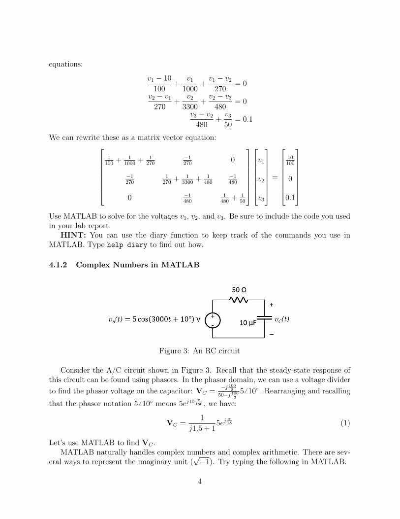
Figure 3: An RC circuit
Consider the A/C circuit shown in Figure 3. Recall that the steady-state response ofthis circuit can be found using phasors. In the phasor domain, we can use a voltage divider
to find the phasor voltage on the capacitor: VC =−j 100
3
50−j 1003
56 10. Rearranging and recalling
that the phasor notation 5 6 10 means 5ej10π
180 , we have:
VC =1
j1.5 + 15ej
π18 (1)
Let’s use MATLAB to find VC .MATLAB naturally handles complex numbers and complex arithmetic. There are sev-
eral ways to represent the imaginary unit (√−1). Try typing the following in MATLAB.
4
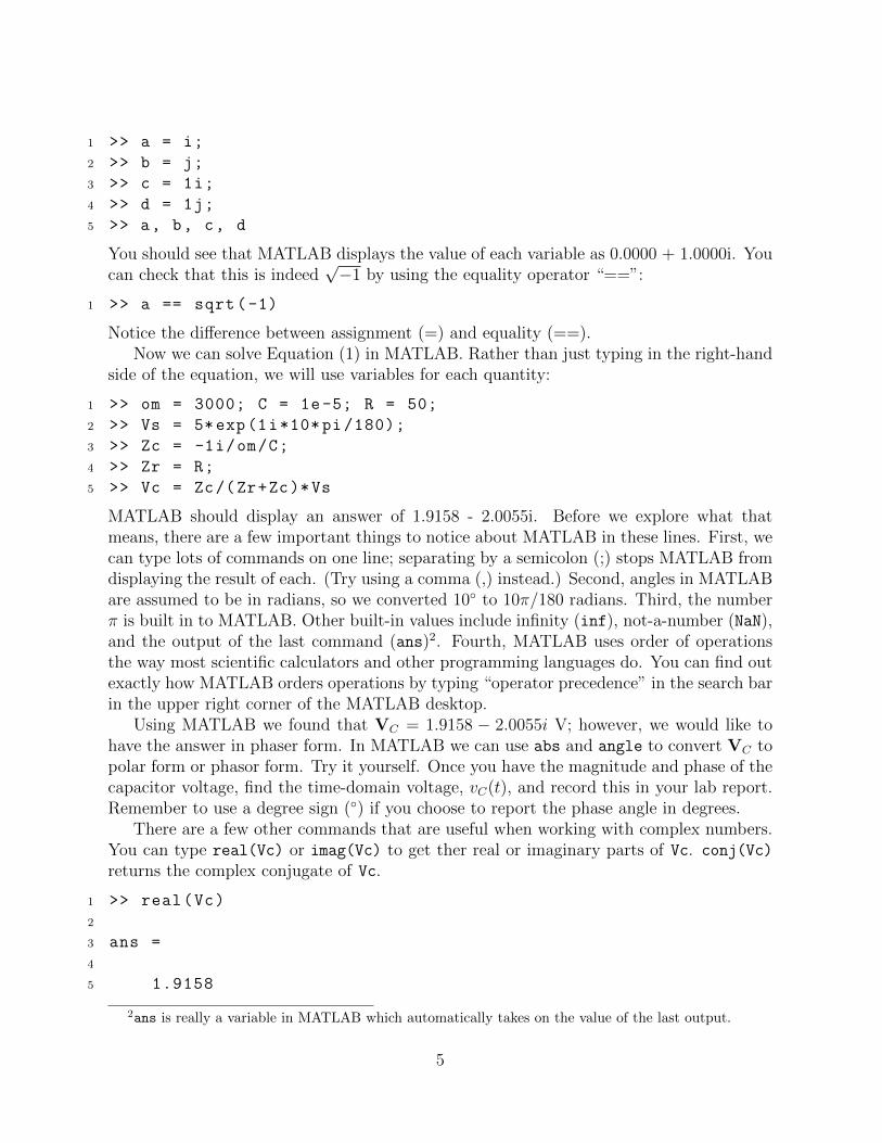
1 >> a = i;
2 >> b = j;
3 >> c = 1i;
4 >> d = 1j;
5 >> a, b, c, d
You should see that MATLAB displays the value of each variable as 0.0000 + 1.0000i. Youcan check that this is indeed
√−1 by using the equality operator “==”:
1 >> a == sqrt(-1)
Notice the difference between assignment (=) and equality (==).Now we can solve Equation (1) in MATLAB. Rather than just typing in the right-hand
side of the equation, we will use variables for each quantity:
1 >> om = 3000; C = 1e-5; R = 50;
2 >> Vs = 5*exp(1i*10*pi /180);
3 >> Zc = -1i/om/C;
4 >> Zr = R;
5 >> Vc = Zc/(Zr+Zc)*Vs
MATLAB should display an answer of 1.9158 - 2.0055i. Before we explore what thatmeans, there are a few important things to notice about MATLAB in these lines. First, wecan type lots of commands on one line; separating by a semicolon (;) stops MATLAB fromdisplaying the result of each. (Try using a comma (,) instead.) Second, angles in MATLABare assumed to be in radians, so we converted 10 to 10π/180 radians. Third, the numberπ is built in to MATLAB. Other built-in values include infinity (inf), not-a-number (NaN),and the output of the last command (ans)2. Fourth, MATLAB uses order of operationsthe way most scientific calculators and other programming languages do. You can find outexactly how MATLAB orders operations by typing “operator precedence” in the search barin the upper right corner of the MATLAB desktop.
Using MATLAB we found that VC = 1.9158 − 2.0055i V; however, we would like tohave the answer in phaser form. In MATLAB we can use abs and angle to convert VC topolar form or phasor form. Try it yourself. Once you have the magnitude and phase of thecapacitor voltage, find the time-domain voltage, vC(t), and record this in your lab report.Remember to use a degree sign () if you choose to report the phase angle in degrees.
There are a few other commands that are useful when working with complex numbers.You can type real(Vc) or imag(Vc) to get ther real or imaginary parts of Vc. conj(Vc)
returns the complex conjugate of Vc.
1 >> real(Vc)
2
3 ans =
4
5 1.9158
2ans is really a variable in MATLAB which automatically takes on the value of the last output.
5

6
7 >> imag(Vc)
8
9 ans =
10
11 -2.0055
12
13 >> conj(Vc)
14
15 ans =
16
17 1.9158 + 2.055i
4.1.3 Vectorization
MATLAB is optimized for operations involving matrices and vectors. For example, wecould use the following code to multiply matrices A and B and store the result in matrixC (assuming C has been initialized to all zeros):
1 >> for x = 1:size(A,1)
2 >> for y = 1:size(B,2)
3 >> for z = 1:size(A,2)
4 >> C(x,y) = C(x,y) + A(x,z) * B(z,y);
5 >> end
6 >> end
7 >> end
Not ony is this annoying to type, but it also executes less efficiently than simply typing:
1 >> C = A*B;
Likewise, matrix-vector products can be found by typing y = H*x for matrix H and vectorsx and y. We can multiply matrices or vectors by scalars by simply typing a*H or a*y.Almost all MATLAB operations are designed to be applied to matrices. In fact, it isgood programming practice to avoid for loops in MATLAB (though sometimes they areunavoidable).
Let’s use vectorization to our advantage. Suppose we want to know the steady-stateoutput voltage VC for the circuit in Figure 3 for the following input voltages:
• vS(t) = 5 cos (3000t+ 10) V
• vS(t) = 5 cos (3000t+ 20) V
• vS(t) = 10 cos (3000t+ 25) V
• vS(t) = 15 cos (3000t) V
6

Since all the sources have the same frequency (3000 radians/s), we can convert these tophasors and vectorize Equation (1):
1 >> Vs = [5* exp(1i*10*pi /180); 5*exp(1i*20*pi /180); ...
2 10* exp(1i*25*pi /180); 15];
3 >> Vc = Zc/(Zr+Zc)*Vs
This creates a column vector of source voltages in phasor form, Vs, and a column vector ofcapacitor voltages in phasor form, Vc. (The ellipsis (...) allows you to write one MATLABcommand on multiple lines.) We have solved all four circuit analysis problems at once! Useabs and angle to convert the answers to the time domain and record these in your report.
4.2 Working with Signals in MATLAB
Strictly speaking, MATLAB (and digital computers in general) can only operate on discrete-time, discrete-amplitude signals. Furthermore, digital computers can only store a finitenumber of signal values at a time. Recall that a signal is a function of one or more inde-pendent variables, and those independent variables are integers for discrete-time signals.
Consider the discrete-time signal x[n] = cos (2π0.01n). We can represent this signal asa vector in MATLAB for the range of integers n = 0, 1, 2, . . . , 9 as follows:
1 >> n = 0:9;
2 >> x = cos (2*pi *0.01*n)
The ten values stored in the array x should display as a row vector. We can change this toa column vector using an apostrophe (’):
1 >> y = x’
MATLAB indexes arrays starting with the number 1, not the the number 0 as manyother programming languages do. (This can be confusing if you are used to C/C++ orJava.) Thus, typing x(1) in MATLAB will display 1.0000, which is equal to cos (2π0.01(0)),whereas typing x(0) will result in an error. As you saw in the documentation for the colonoperator in Section 4.1, you can access various subsets of the vector x as follows:
1 >> x(4:7)
2
3 ans =
4
5 0.9823 0.9686 0.9511 0.9298
6
7 >> x(1:2: end)
8
9 ans =
10
11 1.0000 0.9921 0.9686 0.9298 0.8763
12
7

13 >> x(2:2: end)
14
15 ans =
16
17 0.9980 0.9823 0.9511 0.9048 0.8443
These are the fourth through seventh, odd-numbered, and even-numbered elements of thevector x, respectively.
4.2.1 Plotting Signals
Often signals of interest are functions of time. In the discrete-time case, the integers thatindex a signal correspond to different points in time. Let’s create another signal:
1 >> t = -0.01:1/44100:0.01;
2 >> x = cos (2*pi *440*t); % Don ’t forget the semicolon!
The first line created an array called t, which we are using to store values of time in seconds.The second line created an array called x, which holds the values of our signal as a functionof time.
MATLAB includes many built-in functions for plotting. We will start with the simplest:plot.
1 >> figure; plot(t,x)
The command figure opens up a new figure window. It is good practice to use figure
before plot; otherwise the plot command will use the last figure window that was used andoverwrite whatever was plotted there. The plot command plots the values in array x as afunction of the values in array t. What happens if you omit t? Type the following to findout:
1 >> figure; plot(x)
Describe what happens in your lab report.Let’s recreate the first plot and add some labels.
1 >> figure; plot(t,x)
2 >> xlabel(‘time (s)’)
3 >> ylabel(‘amplitude (V)’)
4 >> title(‘A plot of voltage vs. time ’)
Describe what xlabel, ylabel, and title do in your lab report. Make sure to label yourgraphs in all your lab reports!
We can plot more than one signal on the same figure. Let’s add a sinusoid at a lowerfrequency and amplitude. Use the hold command to add the new signal to the plot.
1 >> hold on
2 >> y = 0.5* cos(2*pi *349.23*t);
3 >> plot(t,y)
8

Using hold on allows us to plot a new signal without erasing the signals already on theplot. If you type hold off, the figure will no longer keep the existing signals when youtype plot. Typing hold by itself toggles the state.
Instead of plotting these two signals on top of each other, we can plot them in separatewindows in the same figure using the subplot command. Let’s plot these two signals andtheir sum:
1 >> figure;
2 >> subplot (3,1,1)
3 >> plot(t,x)
4 >> xlabel(‘time (s)’), ylabel(‘voltage (V)’)
5 >> subplot (3,1,2)
6 >> plot(t,y)
7 >> xlabel(‘time (s)’), ylabel(‘voltage (V)’)
8 >> subplot (3,1,3)
9 >> plot(t,x+y)
10 >> xlabel(‘time (s)’), ylabel(‘voltage (V)’)
11 >> title(’Three signals in subplots ’)
The first two arguments to subplot specify the layout of windows within the figure. Inour example, subplot(3, 1, n) specifies a three by one layout, so we have three subplotsin a column. The third number, n, specifies which of the subplots to use. For rectangularlayouts, n itemizes subplots by column (so subplot(3,2,4) would plot in the upper rightof a three by two layout).
MATLAB offers a lot more plotting functionality. Step through the “Creating 2-DPlots” live demo to see some examples. (Type “demo” in MATLAB to display availabledemos in the help window if it is not still open.) Other useful plotting commands includesemilogx, semilogy, loglog, and axis. Use help to learn about these.
The plot command connects each data point with a straight line, making a signal appearto be continuous-time. What plotting command from the demo could you use to emphasizethat a signal is discrete-time? Explain your answer in your report.
4.2.2 Sounds
Note: MATLAB’s ability to play sounds through speakers or headphones depends on howthe host system is configured. If you are trying this on your own machine, you may needto change the settings.
Signals representing sound and imagery are extremely helpful for developing intuition.Let’s use MATLAB to generate some sounds. A sampling rate of 44.1 kHz is typical formusic. We will learn later in class that this allows recording of music with frequencies upto 22.05 kHz. Most humans cannot hear frequencies above about 20 kHz, so this samplingrate makes sense.
1 >> Fs = 44100; % 44.1 kHz sampling rate
2 >> Ts = 1/Fs; % this is the sampling period or sampling interval
9

3 >> t = -0.5:Ts:0.5;
4 >> x = 0.3* cos (2*pi*440*t);
At this point we have created one second of audio in the vector x. The next command willsend this signal to the speakers at the appropriate sampling rate. Before you hit Enter,be sure to turn the volume down (especially on headphones). You can turn it up latter asnecessary.
1 >> sound(x,Fs)
You should hear one second of a pure ‘A’ (440 Hz).We can make more interesting sounds with the help of some new MATLAB commands.
The commands zeros(m, n) and ones(m, n) are extremely useful. They create m-by-narrays of zeros and ones, respectively:
1 >> zeros (2,5)
2
3 ans =
4
5 0 0 0 0 0
6 0 0 0 0 0
7
8 >> ones (1,3)
9
10 ans =
11
12 1 1 1
We can create a unit step signal using zeros(m, n) and ones(m, n) as follows.
1 >> u = [zeros (1 ,22050) , ones (1 ,22051)];
Notice the notation we used to create the vector u. In general, typing [A, B] will concate-nate the matrices (or vectors) A and B. The comma (,) puts the matrices side-by-side, so A
and B must have the same number of rows for this to work. The semicolon (;) concatenatesmatrices on top of one another (assuming they have the same number of columns).
Now lets make another sound signal using our unit step function.
1 >> y = 0.3* cos(2*pi *349.23*t);
2 >> s = x + u.*y;
The last line adds the vector x to another vector formed by multiplying y by a unit step.The “dot multiply” notation (.*) tells MATLAB to multiple the vectors point-wise ratherthan using a vector product. Now we are ready to play our new signal.
1 >> sound(s,Fs)
Describe what you hear in your lab report.
10

4.2.3 Images
Usually we deal with signals that are a function of one independent variable, such as thesound signals we just created. Signals can be functions of two or more independent variablesas well. Images are two-dimensional signals where the two independent variables are thex and y coordinates. The dependent variable is either a grayscale value or a color (oftenrepresented by three dependent variables: R, G, and B). Future labs will explore imagesand image processing; this section will briefly introduce images in MATLAB.
We can use zeros(m, n), ones(m, n), and concatenation to make a very boring image.
1 >> im = [zeros (20,20), ones (20 ,20); ones (20,20), zeros (20 ,20)];
2 >> figure; imshow(im)
We could make the image a little more exciting by repeating a few times.
1 >> board = repmat(im ,4,4);
2 >> figure; imshow(board)
The command repmat(im,4,4) repeats the matrix im in an four by four grid.Without other arguments, imshow assumes images to be grayscale with zero correspond-
ing to black and one corresponding to white. Color images can be displayed by providinga colormap.
1 >> load clown.mat
2 >> figure; imshow(X,map)
MATLAB also provides the commands image and imagesc to display images. Theseassume color images, but the default colormap is not always appropriate. Pixel valuesshould range from 0 to 255 when using image (assuming a colormap of 256 values). Whenusing imagesc, the pixel values are automatically scaled to fit the colormap.
Try the following commands and explain any differences that you observe betweenimshow, image, and imagesc.
1 >> figure; imshow(X,map)
2 >> figure; image(X)
3 >> colormap(map)
4 >> figure; imagesc(X)
5 >> colormap(map)
4.3 Report Checklist
Be sure the following are included in your report.
1. Section 4.1.1: Code to solve DC circuit and solution
2. Section 4.1.2: Solution for vC(t)
3. Section 4.1.3: Solution for vC(t) for four vS(t) input signals
11

4. Section 4.2.1: Description of what happens when plotting x without t
5. Section 4.2.1: Description of xlabel, ylabel, and title
6. Section 4.2.1: Description of how to emphasize a discrete-time signal in a plot
7. Section 4.2.2: Description of the sound you hear
8. Section 4.2.3: Explanation of the differences you observe
References
[1] MathWorks MATLAB Website. MATLAB, The MathWorks, Inc.,https://www.mathworks.com/products/matlab.html
[2] “MATLAB Installation Instructions.” Iowa State University Information Technology,Iowa State University of Science and Technology,https://www.it.iastate.edu/services/software-students/matlab
[3] Eaton, John W. GNU Octave Website. GNU Octave, John W. Eaton,https://www.gnu.org/software/octave/
[4] Scilab Website. Scilab, ESI Group,https://www.scilab.org/
[5] FreeMat Website. FreeMat, SourceForge,http://freemat.sourceforge.net/
12

Synthesis of Sinusoidal Signals using Tuning Forks
EE 224: Signals and Systems I
1 Overview
Tuning forks are physical systems that generate sinusoidal signals. When a tuning forkis exposed to vibration, it disturbs nearby air molecules, creating regions of higher-than-normal pressure (called compressions) and regions of lower-than-normal pressure (calledrarefactions). A microphone converts these variations to an electrical signal which canbe digitized with an analog-to-digital converter (ADC). The digital signal can be recorded,analyzed, processed, and replayed through a digital-to-analog converter (DAC) and speaker.This lab allows you to analyze sounds produced by tuning forks.
2 Learning Objectives
By the end of this lab, students will be able to:
1. Use the CyDAQ to record data
2. Write and use a MATLAB function
3. Measure the period of a signal
4. Determine the fundamental frequency of a measured signal
3 Pre-Lab Reading
Read the lab manual and the “Getting Started with the CyDAQ” document. Also read theWikipedia on tuning forks (in particular to see how the frequency of a fork is calculated).This lab uses tuning forks with frequencies ranging from 128 Hz to 4096 Hz. Assumingthat the stiffness of the tuning forks is the same, how does the length of a tuning forkchange as the frequency increases? Enter your answer in the Canvas pre-lab and verifyyour hypothesis when you get to the lab.
Do not strike the tuning forks on the table.
13

4 Lab Exercises
4.1 Overview
In this lab, you will be introduced to the CyDAQ, a device created specifically for thiscourse. The CyDAQ is capable of recording signals from a variety of sensors, and storingthe data in a way that can be easily used in MATLAB. For more information, refer to theGetting Started with CyDAQ document on Canvas.
Using a tone generator smartphone app, a pure sinusoidal tone can be generated andrecorded using the microphone on the CyDAQ. In order to observe a decaying signal, atuning fork can also be used. The CyDAQ will convert the generated sound to an electricalsignal, which in turn is converted to a sequence of numbers stored in a digital file whichcan be displayed on computer screen as a sinusoidal curve. Characteristics of the soundwave, such as its period T and frequency f can be determined from this curve. Knowingthe wave’s period, its frequency f is easily computed using the formula:
f = 1/T
4.2 MATLAB Preliminaries
In this section, you will write an m-file function that takes a sound signal at a specificsampling rate and plots the FFT (Fast Fourier Transform) of the signal. You will need toimport the data recorded from the CyDAQ into MATLAB. Your function should take the‘data’ vector imported from the CyDAQ, and the sampling rate, Fs.
4.2.1 Introduction to Using Functions in MATLAB
Functions are m-files that can accept input arguments and return output arguments. Thenames of the m-file and of the function should be the same. Functions operate on variableswithin their own workspace, separate from the workspace you access at the MATLABcommand prompt. The first line of a function m-file starts with the keyword function. Itgives the function name and order of arguments. A simple function, called compmag5 thatcomputes five times the magnitude of a complex number of the form x+ jy is given below.In this case, there are two input arguments and one output argument.
1 function [z] = compmag5(x,y);
2 % % % % % % % % %
3 % this function computes the magnitude of the complex number
4 % x+jy and returns it in variable z.
5 % Inputs:
6 % x - real part of complex number
7 % y - imaginary part of complex number
8 %Outputs:
9 %z - magnitude of complex number times 5
14

10 %written by J.A. Dickerson , January , 2005
11 a=5;
12 % compute magnitude and multiply
13 z = a * sqrt(x^2+y^2);
The next several lines, up to the first blank or executable line, are comment lines thatprovide the help text. These lines are printed when you type
1 >>help compmag5
The first line of the help text is the H1 line, which MATLAB displays when you use thelookfor command or search a directory with MATLAB’s Current Folder browser. The restof the file is the executable MATLAB code defining the function. The variable a introducedin the body of the function, as well as the variables on the first line, m, x and y, are all localto the function; they are separate from any variables in the MATLAB workspace. Thismeans that if you change the values of any variables with the same name while you are inthe function, it does not change the value of the variable in your workspace.
If no output argument is supplied, the result is stored in ans. You can terminate anyfunction with an end statement but, in most cases, this is optional. Functions returnwhen the end of the function is reached. The function is used by calling the functionwithin MATLAB or from a script. For example, the commands below can be used to callcompmag5 and get a result of m = 14.1421.
1 >> x=2; y=2; m=compmag5(x,y);
4.2.2 Writing an FFTPlot Function
For this lab, you will need a function that plots the frequency spectrum of a recorded signal.This function can also be reused in future labs. Using the FFT function in MATLAB willallow you to do so. For more information, refer to the following link: https://www.
mathworks.com/help/matlab/ref/fft.html. Be sure to plot the amplitude spectrumwith amplitude on the y-axis and frequency on the x-axis. You function should take asinput arguments the ‘data’ vector imported from the CyDAQ, and the sampling frequency(Fs) used when collecting the signal.
The following will help you get started:
1 function [] = FFTPlot(data , Fs)
2 % FFTPlot: convert data vector from time domain to frequency
3 % domain
4 % data: imported ‘data ’ vector from the CyDAQ
5 % Fs: sampling frequency specified on the CyDAQ
6
7
8
9 end
15
4.2.3 Labeling Plots in MATLAB
It is very important to label all plots and graphs submitted with your lab report. Recallhow to use the functions xlabel, ylabel, and title from Lab 1. The axis command canbe used to set the beginning and end values for the graph axes. For example, if the timeshould start at 2 s and end at 5 s and the recorded signal should range between 0 and 10volts, use the command axis([2, 5, 0 10]);. Type help axis for more information.
4.3 Signal Collection
A. First, using the CyDAQ, collect signals generated by a tone generator app. Referto the ‘Getting Started with CyDAQ’ document for instructions. Collect the signalsusing a sampling frequency of 8000 Hz on Channel 0, with ‘No Filter’ selected. Selecttwo frequencies greater than 150 Hz and less than 1000 Hz. For each of the selectedfrequencies, plot both the time domain of the signal (plot(time,data)) and thefrequency domain of the signal (FFTPlot(data,Fs)) in the same figure using subplot.Remember to include title and axis labels for both subplots! Include these plots inyour report.
B. Use the data cursor tool to measure the frequency. In the frequency domain plot, thiscan be done by finding the x coordinate of a peak value. In the time domain plot,this can be done by measuring the time difference between two peaks. (The timedifference between two consecutive peaks would give the period.) You may be ableto achieve better accuracy by measuring the time it takes for N peaks to occur, thendividing by N−1. Verify that your two frequency measurements are reasonably closeto each other. How do your measurements compare to the frequency you specifiedin the tone generator? Explain any discrepancies between your measured data andyour expected value.
C. Next, collect tuning fork signals. Use the CyDAQ to collect signals for two differenttuning forks with frequencies at or under 2048 Hz using a sampling frequency of8000 samples/sec. Repeat parts A and B for each of the tuning forks. How do yourmeasurements compare to the frequency listed on the tuning fork you used? Explainany discrepancies between your measured data and the expected frequency. Note: Ifyour measured frequency is not reasonably close to the tuning fork frequency, it ispossible that you are collecting data for too long. With your lab partner, have oneperson strike the tuning fork and one person push start and stop. Stop data collectionwithin three seconds of starting.
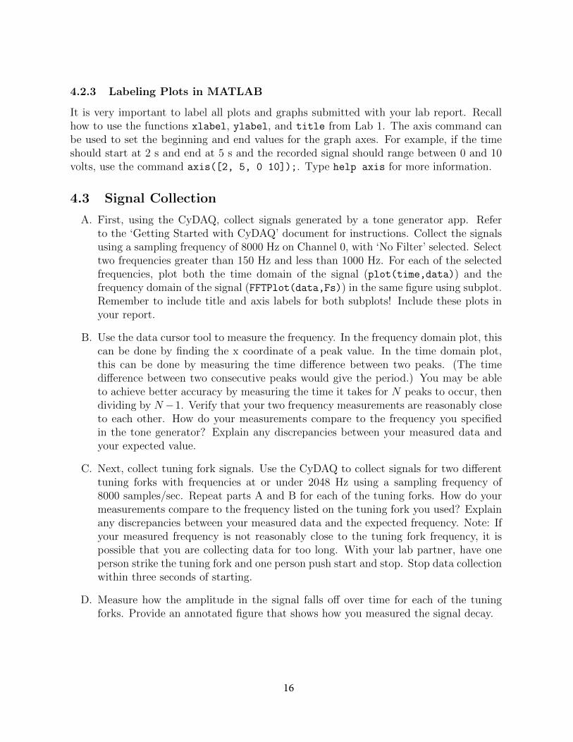
D. Measure how the amplitude in the signal falls off over time for each of the tuningforks. Provide an annotated figure that shows how you measured the signal decay.
16
Figure 1: Example tuning fork recording.
E. Comment on the other signals present in the spectrum. Why don’t you see a niceclean delta function in the frequency plot?
F. Fill in the table below as part of your report. Include entries for the ‘FrequencyEstimate from Time Plot’ and the ‘Frequency Estimate from Frequency Plot’ forboth frequencies from the tone generator as well as the entries for both tuning forks.
Signal SourceFrequency Estimatefrom Time Plot (Hz)
Magnitude DecayRate (V/s)
Frequency Estimatefrom Frequency Plot(Hz)
Tuning forklabeled 1024
Signal genera-tor 440 Hz
N/A
17

4.4 Report Checklist
Be sure the following are included in your report.
1. All your MATLAB code in an appendix of the report (including your FFTPlot func-tion)
2. Section 4.3A.: Time and frequency plots of data measured from a tone generator app
3. Section 4.3C.: Time and frequency plots of data measured from a tuning fork
4. Section 4.3B.: Frequency measurements of the tone generator app’s signal from timeand frequency plots (report in table)
5. Section 4.3C.: Frequency measurements of the tuning fork from time and frequencyplots (report in table)
6. Section 4.3B.: Explanation of discrepancies between measured and expected frequen-cies
7. Section 4.3D.: Plot and measurement of tuning fork amplitude decay (report estimatein table)
8. Section 4.3E.: Comment on other signals in the spectrum
18
Impulse Response and Auralization
EE 224: Signals and Systems I
1 Overview
“Auralization” is the process of using a computer to create or reproduce sound, often toachieve a desired sound effect. This is done by simulating characteristics of a room orother environment in order to produce sound that seems to have been recorded in thatenvironment. Auralization is an increasingly popular technique for accurately simulatingreverberation using acoustic impulse responses (IRs) from interesting buildings, spaces, andother sources. It is also used in video game and film production to create realistic soundeffects.
Bring headphones to this lab!
2 Learning Objectives
By the end of this lab, students will be able to:
1. Use a real-world impulse response to simulate different environments using discrete-time convolution
2. Describe FM modulated signals and chirp signals
3. Interpret a spectogram
3 Pre-Lab Reading
3.1 Auralization and Background
EchoThief (http://www.echothief.com) collects interesting IRs from “unusually clam-orous places” for anyone to use. You can read about how these IRs are created here.A similar process is described in Section 3.1.1 This lab will use the computed impulseresponses to approximate the sound of a signal in different environments.
19
3.1.1 Signal Acquisition
Ideally, we could obtain the acoustic impulse response of a space by producing an impulsesignal and measuring the sound it produces in a given space. Unfortunately, impulsefunctions can only be approximated in the real world. One way to do this is to produce ashort, tall (i.e., loud) pulse, but this requires a large amount of power (equal to the energyof the pulse divided by the pulse width). Requiring both more energy and a shorter pulsemakes electrical power handling a limiting factor in such a system. The output stage of atransmitter can only handle so much power without destroying itself.
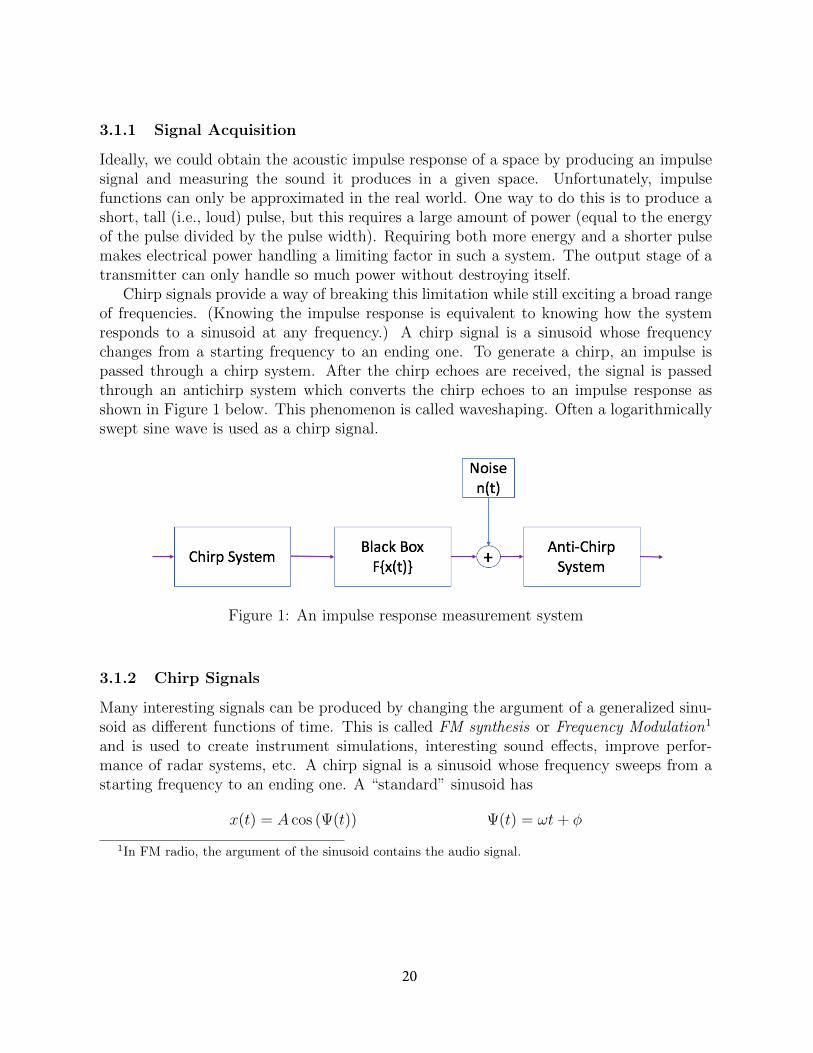
Chirp signals provide a way of breaking this limitation while still exciting a broad rangeof frequencies. (Knowing the impulse response is equivalent to knowing how the systemresponds to a sinusoid at any frequency.) A chirp signal is a sinusoid whose frequencychanges from a starting frequency to an ending one. To generate a chirp, an impulse ispassed through a chirp system. After the chirp echoes are received, the signal is passedthrough an antichirp system which converts the chirp echoes to an impulse response asshown in Figure 1 below. This phenomenon is called waveshaping. Often a logarithmicallyswept sine wave is used as a chirp signal.
Figure 1: An impulse response measurement system
3.1.2 Chirp Signals
Many interesting signals can be produced by changing the argument of a generalized sinu-soid as different functions of time. This is called FM synthesis or Frequency Modulation1
and is used to create instrument simulations, interesting sound effects, improve perfor-mance of radar systems, etc. A chirp signal is a sinusoid whose frequency sweeps from astarting frequency to an ending one. A “standard” sinusoid has
x(t) = A cos (Ψ(t)) Ψ(t) = ωt+ φ
1In FM radio, the argument of the sinusoid contains the audio signal.
20

However, much more interesting signals can be created with different functions such as aquadratic, logarithmic, or sinusoid as shown below.
Ψ(t) = 2πµt2 + 2πf0t+ φ
Ψ(t) = eat + 2πf0t+ φ
Ψ(t) = cos (2πf1t) + 2πf0t+ φ
The frequency spectra of these signals are hard to analyze; however, a decent approxi-mation of signal behavior can be found by looking at the first derivative of the argumentfunction. This is known as the instantaneous frequency, fi, of the signal. The instantaneousfrequency of the linear, quadratic, and logarithmic chirp are:
Linear : fi(t) = f0 + βt β =f1 − f0t1
Quadratic : fi(t) = f0 + βt2 β =f1 − f0t21
Logarithmic : fi(t) = f0βt β =
(f1f0
)1/t1
Figure 2 below shows the linear chirp system. For the problem of auralization, a loga-rithmically swept sinusoid is used.
Figure 2: Impulse response of a linear chirp signal (from Figure 11-10 of The Scientist andEngineers Guide to Signal Processing by Steven W. Smith, [2])
These signals can be generated using the Matlab command chirp.y = chirp(t,f0,t1,f1,‘method’,phi)
The command generates samples of a swept-frequency cosine signal at the time instancesdefined in array t, where f0 is the instantaneous frequency at time 0, and f1 is the instan-taneous frequency at time t1. f0 and f1 are both in hertz. If unspecified, f0 = e−6 forlogarithmic chirp and 0 for all other methods, t1 = 1, and f1 = 100.
21
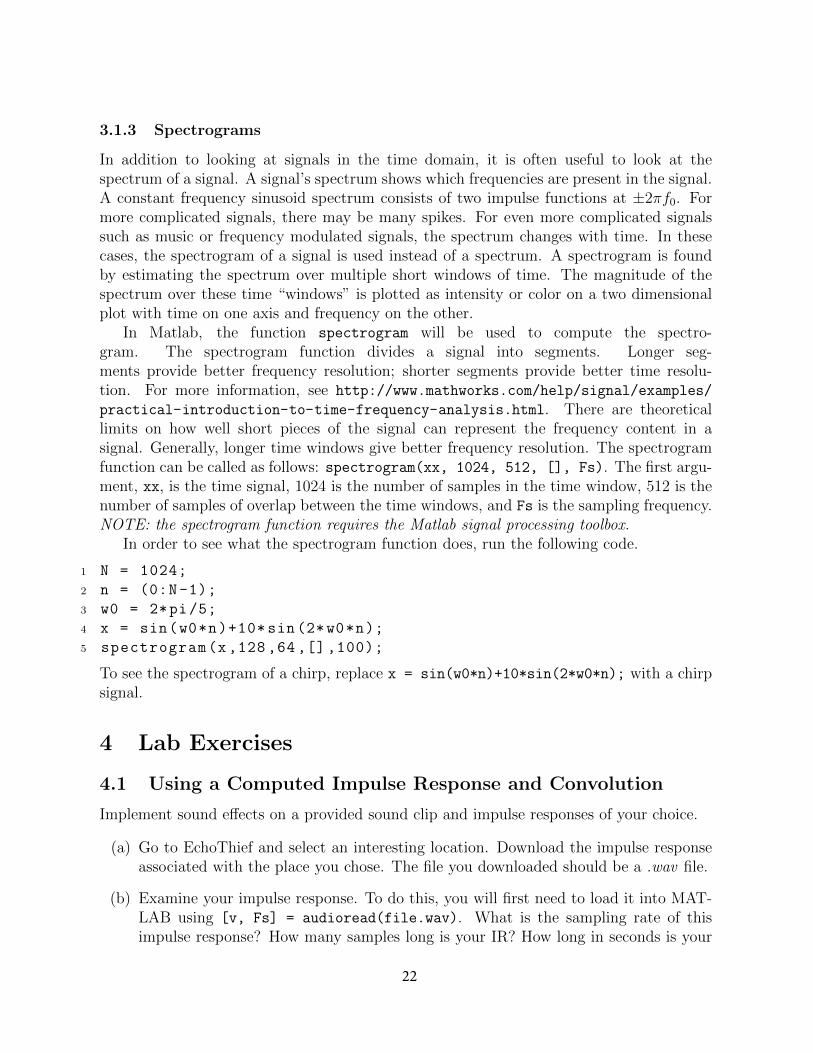
3.1.3 Spectrograms
In addition to looking at signals in the time domain, it is often useful to look at thespectrum of a signal. A signal’s spectrum shows which frequencies are present in the signal.A constant frequency sinusoid spectrum consists of two impulse functions at ±2πf0. Formore complicated signals, there may be many spikes. For even more complicated signalssuch as music or frequency modulated signals, the spectrum changes with time. In thesecases, the spectrogram of a signal is used instead of a spectrum. A spectrogram is foundby estimating the spectrum over multiple short windows of time. The magnitude of thespectrum over these time “windows” is plotted as intensity or color on a two dimensionalplot with time on one axis and frequency on the other.
In Matlab, the function spectrogram will be used to compute the spectro-gram. The spectrogram function divides a signal into segments. Longer seg-ments provide better frequency resolution; shorter segments provide better time resolu-tion. For more information, see http://www.mathworks.com/help/signal/examples/
practical-introduction-to-time-frequency-analysis.html. There are theoreticallimits on how well short pieces of the signal can represent the frequency content in asignal. Generally, longer time windows give better frequency resolution. The spectrogramfunction can be called as follows: spectrogram(xx, 1024, 512, [], Fs). The first argu-ment, xx, is the time signal, 1024 is the number of samples in the time window, 512 is thenumber of samples of overlap between the time windows, and Fs is the sampling frequency.NOTE: the spectrogram function requires the Matlab signal processing toolbox.
In order to see what the spectrogram function does, run the following code.
1 N = 1024;
2 n = (0:N-1);
3 w0 = 2*pi/5;
4 x = sin(w0*n)+10* sin(2*w0*n);
5 spectrogram(x,128 ,64 ,[] ,100);
To see the spectrogram of a chirp, replace x = sin(w0*n)+10*sin(2*w0*n); with a chirpsignal.
4 Lab Exercises
4.1 Using a Computed Impulse Response and Convolution
Implement sound effects on a provided sound clip and impulse responses of your choice.
(a) Go to EchoThief and select an interesting location. Download the impulse responseassociated with the place you chose. The file you downloaded should be a .wav file.
(b) Examine your impulse response. To do this, you will first need to load it into MAT-LAB using [v, Fs] = audioread(file.wav). What is the sampling rate of thisimpulse response? How many samples long is your IR? How long in seconds is your
22

IR? Plot your IR as a function of time, with the time in seconds. Comment on theplot in your report. Is this a mono or stereo recording? You can listen to your IR bytyping soundsc(v, Fs) in MATLAB.
(c) Download one of the two voice files from Canvas (female voice: spfe49 1.wav or malevoice: spme50 1.wav). Load this audio file into MATLAB. What is the sampling rateof this file? Is this a mono or stereo recording? How many samples are in the signal?Listen to the audio. What is the voice talking about?
(d) Now for the fun part! We want to make it sound like the voice is coming from thelocation corresponding to your IR. We can do this by convolving the speach signalwith the impulse response. Suppose your voice signal is v[n] and the IR is h[n]. Theconvolution y[n] = v[n] ∗ h[n] will produce a speach signal that sounds like it wasrecorded at the location you picked. It MATLAB, you can type y = conv(v,h) toconvolve the signals.
(i) NOTE 1: make sure your voice signal and IR are recorded at the same samplingrate, otherwise you will need to use resample on one of them.
(ii) NOTE 2: if your voice signal or IR (or both) were recorded in stereo, you willhave to pick one of the two channels to use before calling conv. You can selectthe first column of a matrix h by typing h1 = h(:,1).
(e) You can play back your new voice by typing soundsc(y,Fs).2 Describe what youhear in your report.
(f) Feel free to experiment with IRs from different locations and different sound files, butleave enough time to finish Section 4.2.
4.2 Investigating Frequency Modulated (FM) Signals
A chirp signal is also known as a swept frequency cosine. The frequency of the cosinechanges in time. The frequency can change in many different ways as seen in Figure 3for linear and quadratic sweeps. We will focus on a linear sweep where the instantaneousfrequency is linear as shown in Figure 3a. Figure 3b shows the case where the instantaneousfrequency is a quadratic.
(a) Use the Matlab chirp command to generate a signal. Find the spectrogram using awindow length of 2048 using the command:
1 spectrogram(x,2048 ,1024 ,[] ,Fs,‘yaxis ’);
Include this plot in your lab report and comment on the shape of the chirp.
2Be sure to use soundsc. The sound function expects to get data ranging from -1.0 to 1.0 (see the helpdocumentation), so if your audio signal exceeds 1.0 in magnitude, you will here additional distortion notcaused by your IR.
23
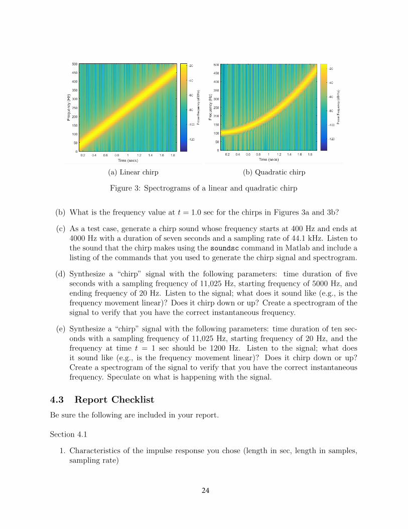
(a) Linear chirp (b) Quadratic chirp
Figure 3: Spectrograms of a linear and quadratic chirp
(b) What is the frequency value at t = 1.0 sec for the chirps in Figures 3a and 3b?
(c) As a test case, generate a chirp sound whose frequency starts at 400 Hz and ends at4000 Hz with a duration of seven seconds and a sampling rate of 44.1 kHz. Listen tothe sound that the chirp makes using the soundsc command in Matlab and include alisting of the commands that you used to generate the chirp signal and spectrogram.
(d) Synthesize a “chirp” signal with the following parameters: time duration of fiveseconds with a sampling frequency of 11,025 Hz, starting frequency of 5000 Hz, andending frequency of 20 Hz. Listen to the signal; what does it sound like (e.g., is thefrequency movement linear)? Does it chirp down or up? Create a spectrogram of thesignal to verify that you have the correct instantaneous frequency.
(e) Synthesize a “chirp” signal with the following parameters: time duration of ten sec-onds with a sampling frequency of 11,025 Hz, starting frequency of 20 Hz, and thefrequency at time t = 1 sec should be 1200 Hz. Listen to the signal; what doesit sound like (e.g., is the frequency movement linear)? Does it chirp down or up?Create a spectrogram of the signal to verify that you have the correct instantaneousfrequency. Speculate on what is happening with the signal.
4.3 Report Checklist
Be sure the following are included in your report.
Section 4.1
1. Characteristics of the impulse response you chose (length in sec, length in samples,sampling rate)
24

2. Plot of your IR and comments about it
3. Description of the voice you chose (sampling rate, mono/stero, number of samples,etc.)
4. Description of your sound effect
Section 4.2
1. Plot of your chirp with comments
2. Frequency values from Figure 3
3. Spectrogram of seven second chirp with code in the appendix
4. Description of five second chirp with spectrogram
5. Description of ten second chirp with spectrogram
References
[1] “EchoThief Impulse Response Library,” EchoThief, SuperHoax,http://www.echothief.com/
[2] Steven W. Smith. The Scientist and Engineer’s Guide to Digital Signal Processing,California Technical Publishing, San Diego, CA, 1997.
[3] Michael Vorlander. Auralization : Fundamentals of Acoustics, Modelling, Simulation,Algorithms and Acoustic Virtual Reality, Springer, Berlin, Germany, 2008.
25
Frequency Response: Notch and Bandpass Filters
EE 224: Signals and Systems I
1 Overview
The goal of this lab is to study the response of finitie impulse response (FIR) filters to inputssuch as complex exponentials and sinusoids. In the experiments, you will use MATLAB’sconv function to implement filters in the time domain and freqz to obtain each filter’sfrequency response. As a result, you should learn how to characterize a filter by knowinghow it reacts to different frequency components in the input. This lab also introducestwo practical filters: bandpass filters and nulling filters. Bandpass filters can be used todetect and extract information from sinusoidal signals, e.g., tones in a touch-tone telephonedialer. Nulling filters can be used to remove sinusoidal interference, e.g., jamming signalsin a radar or 60 Hz power signals from lights.
2 Learning Objectives
By the end of this lab, students will be able to:
1. Plot the frequency response of an FIR filter
2. Implement and apply an FIR filter in MATLAB
3. Design an FIR filter for nulling frequency components
4. Design an FIR filter for isolating specific frequencies
3 Pre-Lab Reading
3.1 Frequency Response of FIR Filters
The output or response of a filter for a complex sinusoidal input, ejΩ, depends on thefrequency, Ω. Often a filter is described solely by how it affects different input frequencies–this is called the frequency response. For example, the frequency response of the two-point
26

averaging filter
y[n] =1
2x[n] +
1
2x[n− 1]
can be found by using a general complex exponential as an input and observing the outputor response.
x[n] = Aej(Ωn+φ)
y[n] =1
2Aej(Ωn+φ) +
1
2Aej(Ω(n−1)+φ)
= Aej(Ωn+φ) 1
2
(1 + e−jΩ
)= Aej(Ωn+φ)H
(ejΩ)
(1)
In (1) there are two terms, the original input and a term that is a function of Ω. Thissecond term is the frequency response, and it is commonly denoted by H(ejΩ), which inthis case is
H(ejΩ) =1
2
(1 + e−jΩ
)Once the frequency response, H(ejΩ), has been determined, the effect of the filter onany complex exponential may be determined by evaluating H(ejΩ) at the correspondingfrequency. The output signal, y[n], will be the original input complex exponential signaltimes a complex number. The phase of this number imparts a phase shift and the magnitudedescribes the gain applied to the complex exponential. The frequency response of a generalfinite impulse response (FIR) linear, time-invariant system is
H(ejΩ) =M∑k=0
bke−jΩk (2)
In the example above, M = 1 and b0 = b1 = 12.
3.2 MATLAB Function for Frequency Response
MATLAB has a built-in function called freqz for computing the frequency response of adiscrete-time LTI system. The following MATLAB statements show how to use freqz1
to compute and plot both the magnitude (absolute value) and the phase of the frequencyresponse of a two-point averaging system as a function of Ω in the range −π ≤ Ω ≤ π:
1If the output of the freqz function is not assigned, then plots are generated automatically; however,the magnitude is given in decibels which is a logarithmic scale. For linear magnitude plots a separate callto plot is necessary.
27
1 bb = [0.5, 0.5]; \% Filter Coefficients
2 ww = -pi:(pi /100): pi; \% omega
3 HH = freqz(bb , 1, ww);
4 subplot (2,1,1);
5 plot(ww, abs(HH)); axis([-pi,pi ,0 ,1]);
6 subplot (2,1,2);
7 plot(ww, angle(HH)); axis([-pi,pi ,-2,2]);
8 xlabel(‘Normalized Radian Frequency ’)
For FIR filters, the second argument of freqz must always be equal to 1. The frequencyvector ww should cover an interval of length 2π for Ω, and its spacing must be fine enoughto give a smooth curve for H(ejΩ). Note: we will always use capital HH for the frequencyresponse in this lab.
3.3 Periodicity of the Frequency Response
The frequency responses of discrete-time filters are always periodic with period equal to2π. Explain why this is the case by stating a definition of the frequency response and thenconsidering two input sinusoids whose frequencies are Ω and Ω + 2π:
x1[n] = ejΩn
x2[n] = ejΩn+2πn
Notice that x2[n] = x1[n], so the output will be the same for both inputs. Include youranswer in your lab report.
The implication of periodicity is that a plot of H(ejΩ) only needs to extendover the interval −π ≤ n ≤ π or any other interval of length 2π.
4 Lab Exercises
4.1 Frequency Response of the Four-Point Averager
Filters that average input samples over a certain interval are called “running average” filtersor “averagers,” and they have the following form (for an L-point averager):
y[n] =1
L
L−1∑k=0
x[n− k]
In other words, the impulse response of an L-point averager is:
h[n] =
1L
0 ≤ n ≤ L− 1
0 otherwise
28

(a) Use Euler’s formula, (2), and complex number manipulations to show that the fre-quency response for the 4-point running average operator is given by:
H(ejΩ)
=cos (0.5Ω) + cos (1.5Ω)
2e−j1.5Ω (3)
(b) Implement (3) directly in MATLAB and plot the frequency response. Use a vectorthat includes 400 samples between −π and π for Ω. Since the frequency response is acomplex-valued quantity, use abs and angle to extract the magnitude and phase ofthe frequency response for plotting. Plotting the real and imaginary parts of H(ejΩ)is not very informative.
(c) Use freqz in MATLAB to compute H(ejΩ) numerically (from the filter coefficients)and plot its magnitude and phase versus Ω. Include the appropriate MATLAB codeto plot both the magnitude and phase of H(ejΩ) in your lab report’s appendix. Followthe example in Section 3.2. The filter coefficient vector for the 4-point averager isdefined via:
1 bb = 1/4* ones (1,4);
Note: the function freqz(bb,1,ww) evaluates the frequency response for all frequen-cies in the vector ww. It uses the summation in (2), not the formula in (3). The filtercoefficients are defined in the assignment to vector bb. How do your results comparewith part (b)?
4.2 The MATLAB find Function
Often signal processing functions are performed in order to extract information that can beused to make a decision. The decision process inevitably requires logical tests, which mightbe done with if-then constructs in MATLAB. However, MATLAB permits vectorizationof such tests, and the find function is one way to do lots of tests at once. In the followingexample, find extracts all the numbers that “round” to 3:
1 xx = 1.4:0.33:5 , jkl = find(round(xx)==3), xx(jkl)
The argument of the find function can be any logical expression. Notice that find returnsa list of indices where the logical condition is true. See help on relop for information.
Now, suppose that you have a frequency response:
1 ww = -pi:(pi /500): pi; HH = freqz( 1/4* ones(1,4), 1, ww );
Use the find command to determine the indices where HH is zero, and then use thoseindices to display the list of frequencies where HH is zero. Since there might be round-offerror in calculating HH, the logical test should probably be a test for those indices wherethe magnitude (absolute value in MATLAB) of HH is less than some rather small number,e.g., 1 × 10⁻⁶. Compare your answer to the frequency response that you plotted for thefour-point averager in Section 4.1.
29
4.3 Nulling Filters for Rejection
Nulling filters are filters that completely eliminate some frequency component. If thefrequency is Ω = 0 or Ω = π, then a two-point FIR filter will do the nulling. The simplestpossible general nulling filter can have as few as three coefficients. If Ω is the desired nullingfrequency, then the following length-3 FIR filter will have a zero in its frequency responseat Ω = Ωn:
y[n] = x[n]− 2 cos (Ω)x[n− 1] + x[n− 2]
For example, a filter designed to completely eliminate signals of the form Aej0.5πn wouldhave the following coefficients because we would pick the desired nulling frequency to beΩn = 0.5π.
b0 = 1, b1 = −2 cos (0.5π) = 0, b2 = 1
(a) Design a filtering system that consists of the cascade of two FIR nulling filters thatwill eliminate the following input frequencies: Ω = 0.44π, and Ω = 0.7π. For thispart, derive the filter coefficients of both nulling filters.
(b) Generate an input signal x[n] that is the sum of three sinusoids:
x[n] = 5 cos (0.3πn) + 22 cos(
0.44πn− π
3
)+ 22 cos
(0.7πn− π
4
)Make the input signal 150 samples long over the range 0 ≤ n ≤ 149.
(c) Use conv to filter the sum of three sinusoids signal x[n] through the filters designedin part (a). Include the MATLAB code that you wrote to implement the cascade oftwo FIR filters in the appendix.
(d) Make a plot of the output signal and show the first 40 points. Determine (by hand)the exact mathematical formula (magnitude, phase, and frequency) for the outputsignal for n ≥ 5. (Hint: recall that an LTI system alters the magnitude and phase ofsinusoidal inputs.)
4.4 Simple Bandpass Filter Design
The L-point averaging filter is a lowpass filter. Its passband width is controlled by L, beinginversely proportional to L. It is also possible to create a filter whose passband is centeredaround some frequency other than zero. One simple way to do this is to define the impulseresponse of an L-point FIR as:
h[n] =2
Lcos (Ωcn), 0 ≤ n < L
where L is the filter length and Ωc is the center frequency that defines the frequency locationof the passband. For example, we would pick Ωc = 0.44π if we want the peak of the filter’spassband to be centered at 0.44π. The bandwidth of the bandpass filter (BPF) is controlledby L; the larger the value of L, the narrower the bandwidth.
30
(a) Generate a bandpass filter that will pass a frequency component at Ω = 0.44π. Makethe filter length (L) equal to 10. Since we are going to be filtering the signal definedbelow, measure the gain of the filter at the three frequencies of interest: Ω = 0.3π,Ω = 0.44π and Ω = 0.7π.
x[n] = 5 cos (0.3πn) + 22 cos(
0.44πn− π
3
)+ 22 cos
(0.7πn− π
4
)(4)
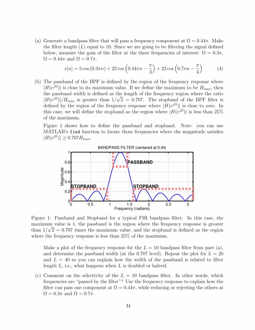
(b) The passband of the BPF is defined by the region of the frequency response where|H(ejΩ)| is close to its maximum value. If we define the maximum to be Hmax, thenthe passband width is defined as the length of the frequency region where the ratio|H(ejΩ)|/Hmax is greater than 1/
√2 = 0.707. The stopband of the BPF filter is
defined by the region of the frequency response where |H(ejΩ)| is close to zero. Inthis case, we will define the stopband as the region where |H(ejΩ)| is less than 25%of the maximum.
Figure 1 shows how to define the passband and stopband. Note: you can useMATLAB’s find function to locate those frequencies where the magnitude satisfies|H(ejΩ)| ≥ 0.707Hmax.
Figure 1: Passband and Stopband for a typical FIR bandpass filter. In this case, themaximum value is 1, the passband is the region where the frequency response is greaterthan 1/
√2 = 0.707 times the maximum value, and the stopband is defined as the region
where the frequency response is less than 25% of the maximum.
Make a plot of the frequency response for the L = 10 bandpass filter from part (a),and determine the passband width (at the 0.707 level). Repeat the plot for L = 20and L = 40 so you can explain how the width of the passband is related to filterlength L, i.e., what happens when L is doubled or halved.
(c) Comment on the selectivity of the L = 10 bandpass filter. In other words, whichfrequencies are “passed by the filter”? Use the frequency response to explain how thefilter can pass one component at Ω = 0.44π, while reducing or rejecting the others atΩ = 0.3π and Ω = 0.7π.
31

(d) Generate a bandpass filter that will pass the frequency component at Ω = 0.44π,but now make the filter length (L) long enough so that it will also greatly reducefrequency components at (or near) Ω = 0.3π and Ω = 0.7π. Determine the smallestvalue of L so that
(a) Any frequency component satisfying |Ω| ≤ 0.3π will be reduced by a factor of10 or more2.
(b) Any frequency component satisfying 0.7π ≤ |Ω| ≤ π will be reduced by a factorof 10 or more.
This can be done by making the passband width very small.
(e) Use the filter from the previous part to filter the “sum of three sinusoids” signal in(4). Make a plot of 100 points of the input and output signals, and explain how thefilter has reduced or removed two of the three sinusoidal components.
(f) Make a plot of the frequency response (magnitude only) for the filter from part (d),and explain how H(ejΩ) can be used to determine the relative size of each sinusoidalcomponent in the output signal. In other words, connect a mathematical descriptionof the output signal to the values that can be obtained from the frequency responseplot.
4.5 Report Checklist
Be sure the following are included in your report.
1. Section 3.3: explanation of periodicity of frequency response
2. Section 4.1: derivation of (3)
3. Section 4.1: (labeled) plots of magnitude and phase of H(ejΩ)
4. Section 4.1: plots of H(ejΩ) using freqz (code in appendix)
5. Section 4.2: list of frequencies where HH is 0 (and compare to above)
6. Section 4.3: coefficients of two nulling filters
7. Section 4.3: MATLAB code for filtering signal (appendix)
8. Section 4.3: plot of nulled output and formula for output signal
9. Section 4.4: coefficients of bandpass filter; gain at three frequencies
2For example, the input amplitude of the 0.7π component is 22, so its output amplitude must be lessthan 2.2
32

10. Section 4.4: plots of frequency response for L = 10, 20, and 40 with a description ofthe passband widths
11. Section 4.4: comments on selectivity of the L = 10 BPF
12. Section 4.4: the smallest L that satisfies the criteria
13. Section 4.4: plot of input and output; explanation of effect on three sinusoid signal
14. Section 4.4: plot of frequency response; explanation of size of each sinusoidal compo-nent in output
33

Fourier Series
EE 224: Signals and Systems I
1 Overview
In this lab you will experience the power of Fourier series analysis and synthesis.
2 Learning Objectives
By the end of this lab, students will be able to:
1. Use MATLAB to approximate Fourier series coefficients of a sampled signal.
2. Use MATLAB to synthesize a signal from its Fourier series coefficients.
3. Describe the difference in sound made by two musical instruments in terms of theirFourier series coefficients.
4. Create your own synthesized instrument using Fourier series (bonus).
3 Pre-Lab Reading
3.1 Fourier Analysis
Begin by reviewing the Fourier analysis formula. Given a periodic signal x(t) with periodT , x(t) can be represented by
x(t) =∞∑
k=−∞
akejkω0t (1)
where ω0 = 2πT
and
ak =1
T
∫ T
0
x(t)e−jkω0tdt for all k (2)
Although an infinite number of harmonics may be required for a general signal, in mostsituations, a finite number of them provides a practically good approximation.
If the signal x(t) is not given as a mathematical function but we have a sampled recordedversion of it, the integrals to compute the coefficients (ak) cannot be evaluated precisely.
34
Although there are more efficient methods to perform the Fourier analysis directly on thesampled signals (e.g., the Fast Fourier Transform (FFT)), we will use a simple method toapproximately evaluate those integrals: the Riemann approximation. Assuming that thesignal x(t) is reasonably smooth (Riemann integrable) and that the sampling time Ts is aninteger fraction of the period T , i.e., T = NTS of samples in a period (this is not reallynecessary but simplifies our code), then:
ak =1
T
∫ T
0
x(t)e−jkω0tdt ' TsT
T/Ts∑n=0
x[Tsn]e−jkω0Tsn. (3)
The approximation gets better and better as the number of samples goes to infinity (mean-ing Ts goes to zero). In other words, fixing the sampling time limits the quality of theapproximation, especially for larger values of k. This is because Ts becomes too large withrespect to kω0, the frequency of the kth harmonic.
Find the Fourier series coefficients a0, a1, a2, and a3 for the square wave given below(assume the signal repeats with period T = 0.04). Use the integral in (3) and include youranswer in your report.
x(t) =
1 0 ≤ t < 0.02
0 0.02 ≤ t < 0.04
3.2 Fourier Synthesis
The synthesis formula allows one to generate periodic signals from the linear combination ofharmonic complex exponentials. Here we assume that the number of non-zero coefficientsak is finite. Then
x(t) =∑k
akejkω0t
In particular,
x[Tsn] =∑k
akejkω0Tsn
4 Lab Exercises
4.1 Fourier Series Analysis Function
Write a Matlab function “findFS” which takes as inputs xT , a vector of samples of x(t)covering one period of x(t); k, the index of the desired coefficient; the period T ; and thesampling time Ts; and produces as output the approximate ak coefficient according to (3).Note that you can easily take advantage of vectorization by considering the product of therow vector xT and the column vector e−jkω0Tsn. A template for the function is provided.
35
4.2 Fourier Series Coefficients of a Square Wave
Let’s construct a test signal. Define in Matlabx T=[ones(1000,1);zeros(1000,1)];
This is one period of a square wave signal. Let the fundamental period be T = 0.04 sec.
a) Calculate the sampling time Ts and explain your answer. (Hint: Ts = T/2000)
b) Use the function you wrote in the previous exercise to compute a0, a1, a2, and a3.
c) Find a−1, a−2, and a−3. How do these relate to a1, a2, and a3?
d) Verify the coefficients you have computed approximate reasonably well the actualcoefficients you obtained for the prelab.
4.3 Fourier Series Synthesis
Write a Matlab function “synthFS” which has the following inputs: a column vector C =[a0; a1; . . . ; am] of coefficients where m is the largest integer corresponding to a non-zerocoefficient, the sampling time Ts, and the fundamental period T . The output should bexT (Tsn), the vector of N = T/Ts (N an integer) samples corresponding to one period of x.Note that your program should verify that T/Ts is an integer. You will also need to extendC to include the complex conjugate coefficients corresponding to the negative ks. Finally,you may want to generate an array F whose columns are the vectors ejkω0Tsn. xT is thencomputed as F*CC, where CC is a vector containing all the coefficients from −m to m. Atemplate for this function is provided.
4.4 Spectra of a Trumpet and Whistle
Load the data file trumpet whistle.mat, which can be found on Canvas. It containsvectors trumpet and whistle. Both signals are sampled at f0 = 44100 Hz, and theyrepresent one period of synthetic trumpet and whistle tones generated by a toy electrickeyboard.
a) Compute the period of the two signals.
b) For each signal, compute and report the first 9 harmonic coefficients, i.e., aks withk = −9, . . . , 9 using the function “findFS” you have developed.
c) For each signal, plot the magnitude and phase spectra of the frequency componentsfrom part b. Briefly comment on their main differences. You may use the Matlabfunction stem to plot the spectrum.
d) For each signal, synthesize an approximation by using the periods in part a, thecoefficients in part b, the sampling time Ts = 1/f0, and your function “synthFS.”
36
e) For each signal, plot on the same plot the given signal and its synthesized approxi-mation. (You may use spectraplot.m found on Canvas. Make sure the axis labelsare accurate.) Comment on the quality of the approximation in both cases.
f) For each signal and its approximation, generate a new signal by repeating them for1000 periods (e.g., using the built in function repmat). Use the function sound inMatlab and the sampling frequency f0 to hear the sound you have generated. Canyou hear the difference between the originals and the approximations? Comment.(Note you may need to scale the signals to have magnitude 1, see help sound.)
Note that the trumpet sound has a much richer spectrum and corresponds to a more com-plex sound. While the whistle sound essentially does not have any harmonic componentsabove the ninth and does not have any even harmonic components, the trumpet sound hasimportant harmonics above the ninth; this can be argued from the error in the approxima-tion.
4.5 Bonus
Synthesize your own “instrument” by repeating steps d-f of the last subsection. Insteadof using the ak that you calculated for the trumpet and whistle, come up with your owncoefficients any way you want. (You don’t have to limit yourself to nine coefficients.)Upload your sound and describe it in your report.
4.6 Report Checklist
Be sure the following are included in your report.
1. Section 4.1: include your function in the appendix
2. Section 4.2: provide answers for a-d
3. Section 4.3: include your function in the appendix
4. Section 4.4: provide answers for a-c, e, and f
5. Section 4.5: (bonus) describe the sound you created and explain how you created it
37

Introduction to Digital Images
EE 224: Signals and Systems I
1 Overview
In this lab we introduce digital images as a new higher dimensional signal type. Digitalimages are written as two-dimensional matrices of numbers that can be manipulated toenhance contrast, invert images, and highlight objects.
2 Learning Objectives
By the end of this lab, students will be able to:
1. Describe digital image types, including monochrome and color.
2. Display images in MATLAB.
3. Perform basic pixel manipulation including clearing, copying, inverting, and thresh-olding.
4. Perform grsyscale brightening and contrast-stretching.
3 Pre-Lab Reading
3.1 Monochrome Images
An image can be represented as a function J(x, y) of two continuous variables representingthe horizontal (x) and vertical (y) coordinates of a point in space. The variables x andy represent spatial dimensions. Thus, their units would be inches or some other unit oflength. Moving images (such as video) add a time variable to the two spatial variables.Digital images sample the signal J(x, y) at uniform intervals:
J [m,n] = J(mT1, nT2) 1 ≤ m ≤M and 1 ≤ n ≤ N
where T1 and T2 are the sample spacings in the horizontal and vertical directions. InMATLAB, we can represent an image as a matrix which consists of M rows and N columns.
38

The matrix entry at (m,n) is the sample value J [m,n]called a pixel (short for pictureelement).
Monochrome images are displayed using black and white and shades of gray, so they arecalled grayscale images. In this lab, we will consider only sampled grayscale still images. Asampled grayscale still image would be represented as a two-dimensional array of numbers.An important property of light images such as photographs and TV pictures is that theirvalues are always non-negative and finite in magnitude; i.e.,
0 ≤ J [m,n] ≤ Jmax <∞
This is because light images are formed by measuring the intensity of reflected or emittedlight which must always be a positive, finite quantity. When stored in a computer ordisplayed on a monitor, the values of J [m,n] have to be scaled relative to a maximumvalue Jmax . Usually, an eight-bit integer representation is used. With 8-bit integers,the maximum value (in the computer) would be Jmax = 28 − 1 = 255, and there would be28 = 256 different gray levels for the display, from 0 to 255. Images in this format have typeuint8 (unsigned 8-bit integer) in MATLAB. However, in image recognition applications,binary images (Jmax = 1) are often used to separate parts of the image that are of interestfrom areas that are not. A simple example is the application of zip code recognition onletters. The algorithm would first search for the zip code, then filter out the rest of theimage.
3.2 Displaying and Exporting Images in MATLAB
Most of the lab exercises in this class will require you to produce one or more outputimages. These will need to be incorporated into your report. Since many exercises will useMATLAB, we will describe here some basic I/O and display commands in the MATLABenvironment.
• Reading Images: You can read an image file, img.tif or image.jpg, into the MATLABworkspace using the command:
1 IMG=imread( p o u t . t i f );
This will produce an image matrix IMG of data type uint8.
• Displaying Images: You can display the image array IMG with the following com-mands.
1 colormap(gray (256)); % only needed for grayscale image
2 imshow(IMG)
3 truesize;
If IMG is a grayscale image, the colormap function is needed to tell MATLAB whichcolor to display for each possible pixel value. The truesize command, which isincluded in the image processing toolbox, maps each image pixel to a single displaypixel to avoid any interpolation on the display. This will be important in future labs.
39
• Writing Images: When producing a lab report document, you should strive to presentthe best representation of your output images. Therefore, it is best to export yourimages to a lossless file format, such as TIFF or BMP, which can then be importedinto your lab report document. You can write the image array X to a file using theimwrite function:
1 imwrite(x, i m g _ o u t . t i f )
Note that if X is of type uint8, the imwrite function assumes a dynamic range of[0, 255], and will clip any values outside that range. If X is of type double, thenimwrite assumes a dynamic range of [0, 1], and will linearly scale to the range [0, 255],clipping values outside that range, before writing out the image to a file. To convertthe image to type uint8 before writing, you can use
1 imwrite(uint8(x), i m g _ o u t . t i f )
If your image is in color, such as RGB (Red-Green-Blue), then you will need toconvert it to grayscale using the rgb2gray command in MATLAB:
1 RGB = imread(‘peppers.png ’); imshow(RGB)
2 I = rgb2gray(RGB);
3 figure; imshow(I)
3.3 Prelab Questions
Open Matlab and run the following command:
1 moon = imread(‘moon.tif ’);
1. What is the size of the image example? NxM pixels
2. What is the variable type?
3. Write out one line of Matlab code for seeing the intensity value of any given pixel inthe image.
4 Image Manipulation
The goal of image manipulation is to improve the image in ways that increase the perfor-mance of a system for human viewing or computer vision applications.
40

Figure 1: Image of a tire with a histogram of intensity values. Most of the pixels have lowintensities.
4.1 Histogram Computation
Image histograms are a simple but very useful method to analyze images and to enhance thequality of the image (at least for a human observer) by performing point transformations.In grayscale images, the histogram looks at the distribution of the intensity values of theimage. For each range of grayscale values, the number of pixels in that range are counted.To see the distribution of intensities in the image, create a histogram by calling the imhist
function. Generally, a good contrast image will have values spread out across the rangeof the intensity values from 0 to N . Figure 1 shows the MATLAB image tire.tif and itshistogram. Note that most of the pixels have low values that are in the range of 0-25 inintensity.
4.2 Contrast Stretching and Intensity Level Slicing
Figure 2: Example contrast mapping s = T (r). The function T is applied to each pixel.
Low contrast images result from poor illumination or lack of response from the imagingsensor. The idea behind contrast stretching is to increase the dynamic range of the gray
41

levels in the image being processed. This is implemented by a mapping function, s = T (r).Figure 2 shows a typical transformation for contrast stretching. The locations of points(r1, s1) and (r2, s2) control the shape of the contrast function. If r1 = r2 and s1 = s2,then the transformation is a linear function. If r1 = r2, s1 = 0, and s2 = L− 1, then thetransformation is a thresholding function. Intermediate values produce different types ofspread. The mapping is a piecewise linear interpolation.
Figure 3: Example mapping functions for Intensity Level Slicing. The mapping on theleft zeros out all pixels that have intensities below A (r < A) and above B (r > B). Themapping on the right brightens pixels with intensities between A and B (A ≤ r ≤ B).
A related transformation is Intensity Level Slicing which can highlight or delete a specificrange of gray levels. Applications include enhancing features such as water in satelliteimages or the tire in the image above. There are two main approaches for this: displaya high value for all of the pixels in a desired range and zero out the others or brightenthe pixels in the range and leave the other pixels the same. Levels can be deleted using asimilar approach. Examples are shown in Figure 3.
4.3 Histogram Equalization
The histogram equalization operation tries to change the pixel distribution so that it is asclose as possible to a uniform distribution. This means that all gray levels from 0 to 2B−1(where B is the number of bits) are approximately equally likely. The effect is to widenthe effective dynamic range of the image intensity. The results for this operation are shownin Figure 4 for the tire.tif image. Compare this to the original image in Figure 1. Notethat the histogram extends across most gray values with approximately equal numbers ofoccurrences. MATLAB code for this operation is (X is the original image):
1 Xeq = histeq(X);
2 figure; subplot (121); imshow(Xeq)
3 subplot (122); imhist(Xeq)
42
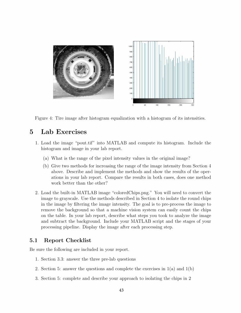
Figure 4: Tire image after histogram equalization with a histogram of its intensities.
5 Lab Exercises
1. Load the image “pout.tif” into MATLAB and compute its histogram. Include thehistogram and image in your lab report.
(a) What is the range of the pixel intensity values in the original image?
(b) Give two methods for increasing the range of the image intensity from Section 4above. Describe and implement the methods and show the results of the oper-ations in your lab report. Compare the results in both cases, does one methodwork better than the other?
2. Load the built-in MATLAB image “coloredChips.png.” You will need to convert theimage to grayscale. Use the methods described in Section 4 to isolate the round chipsin the image by filtering the image intensity. The goal is to pre-process the image toremove the background so that a machine vision system can easily count the chipson the table. In your lab report, describe what steps you took to analyze the imageand subtract the background. Include your MATLAB script and the stages of yourprocessing pipeline. Display the image after each processing step.
5.1 Report Checklist
Be sure the following are included in your report.
1. Section 3.3: answer the three pre-lab questions
2. Section 5: answer the questions and complete the exercises in 1(a) and 1(b)
3. Section 5: complete and describe your approach to isolating the chips in 2
43

References
[1] R.C. Gonzalez and R.E. Woods Digital Image Processing, Addison Wesley, 1993
[2] “MATLAB Image Processing Toolbox Documentation”,’ The Mathworks,https://www.mathworks.com/help/images/index.html?s_tid=CRUX_lftnav
[3] Jackson,Jeff Notes from ECE 482, University of Alabama,http://jjackson.eng.ua.edu/courses/ece482/lectures/LECT01-2.pdf
http://jjackson.eng.ua.edu/courses/ece482/lectures/LECT05-2.pdf
44

Filtering Digital Images
EE 224: Signals and Systems I
1 Overview
In this lab, we introduce linear sliding window filtering of images. The filters work in twodimensions to enhance the image in ways such as averaging out noise or emphasizing edges.
2 Learning Objectives
By the end of this lab, students will be able to:
1. Describe spatial frequency in 2D digital images.
2. Design and implement linear, spatially invariant (LSI) filters using two-dimenionalconvolutional windows.
3. Use the properties of LSI filters to implement the Canny Edge Detection Protocol forimages.
3 Pre-Lab Reading and Exercises
3.1 Image Filtering and Spatial Frequency
Image analysis deals with techniques for extracting information from images. The first stepis generally to segment an image. Segmentation divides an image into its constituent partsor objects. For example, in a military air-to-ground target acquisition application one maywant to identify tanks on a road. The first step is to segment the road from the rest of theimage and then to segment objects on the road for possible identification. Segmentationalgorithms are usually based on one of two properties of gray-level values: discontinuityand similarity. For discontinuity, the approach is to partition an image based on abruptchanges in gray level. Objects of interest are isolated points, lines, and edges.
An edge is the boundary between two regions with relatively distinct gray-level proper-ties. The idea underlying most edge-detection techniques is the computation of a relativederivative operator. Figure 1 illustrates this concept. The picture on the left shows an
45

Figure 1: Synthetic images with horizontal pixel intensity, first derivative of intensity, andsecond derivative of intensity.
image of a light stripe on a dark background, the gray-level profile of a horizontal scanline, and the first and second derivatives of the profile. The first derivative is positive whenthe image changes from dark to light and zero where the image is constant. The secondderivative is positive for the part of the transition associated with the dark side of theedge and negative for the transition associated with the light side of the edge. Thus, themagnitude of the first derivative can be used to detect the presence of an edge in the imageand the sign of the second derivative can be used to detect whether a pixel lies on the lightor dark side of the edge.
3.2 Sliding Window Filters
One way of filtering is to first filter the rows with a one-dimensional filter and then filterthe columns with a one-dimensional filter. Alternatively, two dimensional filters can beapplied to the neighborhood of each pixel to filter a signal. Filtering can help remove noisefrom an image by averaging out the effects of random noise fluctuations. High pass filtershelp detect edges and sudden spatial changes in an image.
The operations take place in the spatial domain and operate directly on pixel values.The general form for operations is: y(i, j) = T [x(i, j)] where x(i, j) is the input image,y(i, j) is the filtered output image, T is an operator on x defined over a neighborhoodof point (i, j). The operator, T , defines the size of the neighborhood around each pixel.The neighborhood is usually rectangular, centered on (i, j) and is much smaller than theimage. This neighborhood is moved around to each pixel, hence the name sliding windowor spatial mask. Use of spatial masks for filtering is called spatial filtering and the maskscan be linear or nonlinear. As a note, the linear filter is equivalent to a two-dimensionalconvolution of the image with the filter.
46

Figure 2: Spatial filtering with a sliding window; (left) three by three neighborhood of pixel(i, j); (right) three by three spatial mask.
A three by three linear filter can be written in matrix form as:w1,1 w1,0 w1,−1
w0,1 w0,0 w0,−1
w−1,1 w−1,0 w−1,−1
The output of applying a three by three mask to image x is given by the two-dimensionalconvolution:
y(i, j) =1∑
k=−1
1∑l=−1
wk,lx(i− k, j − l)
= w1,1x(i− 1, j − 1) + w1,0x(i− 1, j) + w1,−1x(i− 1, j + 1)
+ w0,1x(i, j − 1) + w0,0x(i, j) + w0,−1x(i, j + 1)
+ w−1,1x(i+ 1, j − 1) + w−1,0x(i+ 1, j) + w−1,−1x(i+ 1, j + 1)
This masking process continues until all pixels in the image are covered. The standardpractice is to create a new image with the new values. For pixels near the boundary of theimage, the output may be computed using partial neighborhoods or by padding the inputappropriately by adding in repeated edge rows/columns or by a frame of black or whitepixels.
These types of spatial filters are linear and spatially invariant (LSI). They can alsobe interpreted in the frequency domain. Lowpass filters attenuate (or eliminate) high fre-quency components characterized by edges and sharp details in an image with the net effect
47

of blurring the image. Highpass filters attenuate (or eliminate) low frequency componentssuch as slowly varying characteristics. The overall effect is a sharpening of edges. Bandpassfilters attenuate (or eliminate) a given frequency range of frequencies. This is primarilyused for image restoration.
3.3 Technical Notes for Implementing Filter Masks
In this lab, the MATLAB routine imfilter will be used: Y = imfilter(X,h); where Xis the image to be filtered, h is the filter in matrix form, and Y is the filtered image. Asimple example for a three by three averaging filter is given below:
1 >>X=imread( m o o n . t i f );
2 >>h = ones (3)/9;% or [1,1,1;1 1 1;1 1 1]/9;
3 >>Y = imfilter(X,h);
There are two things to keep in mind with imfilter. First, it returns an image inthe same format as the input. This means that if, for a uint8 image, the function gets anon-integer value, it rounds it to the closest integer. Second, it clips pixel values outside ofthe range [0, 255] to 0 or 255. These are non-linear operations which effect whether the LSIoperations can be done in any order. For pixels near the boundary of the image, the outputmay be computed using partial neighborhoods or by padding the input appropriately byadding in repeated edge rows/columns or by a frame of black or white pixels. The defaultin imfilter is to assume a black border. Details can be found by reading about paddingoptions on the help page.
3.4 Pre-Lab Questions
1. Which part of the image in Figure 3 has the lowest spatial frequency: specify top,bottom, left, right, middle, or a corner.
48
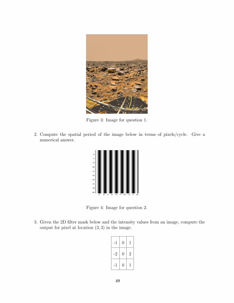
Figure 3: Image for question 1.
2. Compute the spatial period of the image below in terms of pixels/cycle. Give anumerical answer.
Figure 4: Image for question 2.
3. Given the 2D filter mask below and the intensity values from an image, compute theoutput for pixel at location (3, 3) in the image.
-1 0 1
-2 0 2
-1 0 1
49

Pixel # 1 2 3 4 5 6
1 5 25 25 30 20 10
2 20 20 30 60 25 30
3 35 30 40 70 40 40
4 80 80 70 70 60 50
4 Lab Exercises
This part of the lab will be done using the three images that were provided with the lab.They are called I, Ig, and Isp. For each piece of the lab, you will need to display the entireimage before and after filtering. The command for this is:
1 >> imshowpair(I,filtI ,‘montage ’)
You will also need to display a close up of parts of the image that illustrate the filter effectwell. To do this, it helps to display the image with the pixels numbered to help selectthe proper subimage. If the routine imshow does not do this automatically, then use thefollowing code to display image I, for example:
1 >> RI = imref2d(size(I)); figure; imshow(I,RI);
Load the Matlab file matlab.mat with the images.
4.1 Low-Pass Spatial Filtering with a Moving Average Filter
A simple three by three or N = 3 averaging filter has the form:
19
19
19
19
19
19
19
19
19
Write out the 2D filter for the N = 5 case. For averaging filters, the sum of the weightsover the filter should be equal to 1. Use filters with dimensions N = 5, 9, and 13 to filterthe image I. What is the effect of increasing the filter size in parts of the image with smalldetails? Include your output images in your report.
50
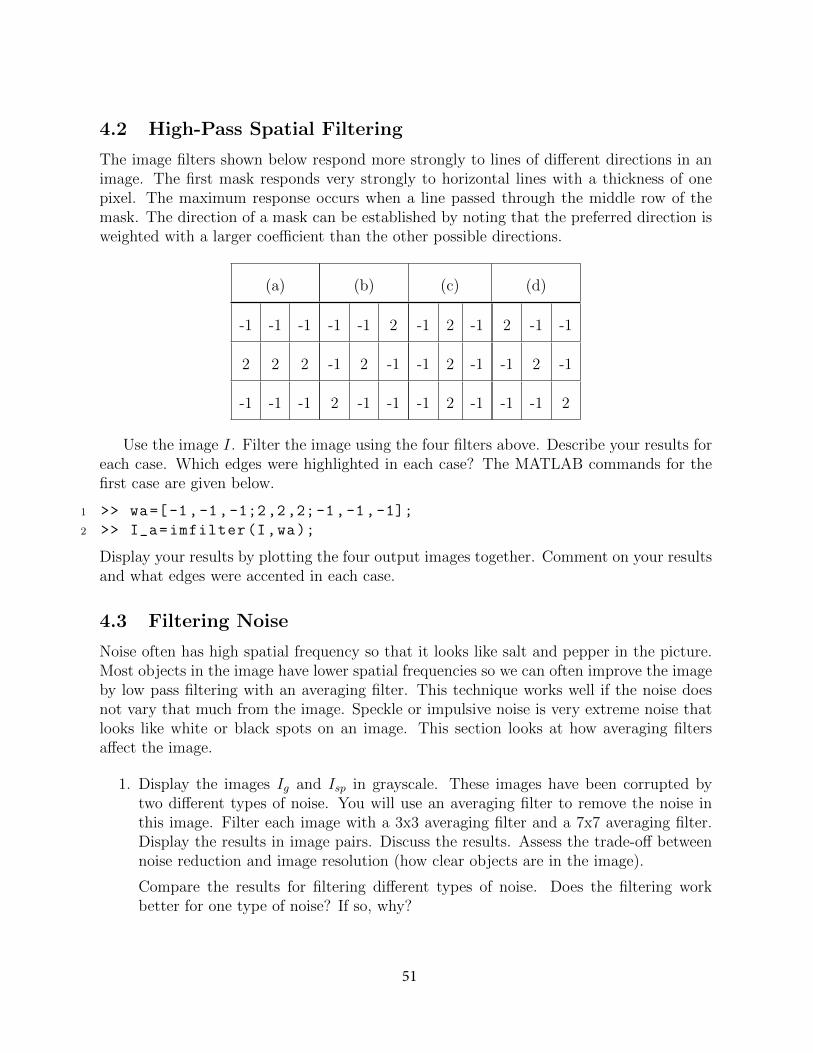
4.2 High-Pass Spatial Filtering
The image filters shown below respond more strongly to lines of different directions in animage. The first mask responds very strongly to horizontal lines with a thickness of onepixel. The maximum response occurs when a line passed through the middle row of themask. The direction of a mask can be established by noting that the preferred direction isweighted with a larger coefficient than the other possible directions.
(a) (b) (c) (d)
-1 -1 -1 -1 -1 2 -1 2 -1 2 -1 -1
2 2 2 -1 2 -1 -1 2 -1 -1 2 -1
-1 -1 -1 2 -1 -1 -1 2 -1 -1 -1 2
Use the image I. Filter the image using the four filters above. Describe your results foreach case. Which edges were highlighted in each case? The MATLAB commands for thefirst case are given below.
1 >> wa=[-1,-1,-1;2,2,2;-1,-1,-1];
2 >> I_a=imfilter(I,wa);
Display your results by plotting the four output images together. Comment on your resultsand what edges were accented in each case.
4.3 Filtering Noise
Noise often has high spatial frequency so that it looks like salt and pepper in the picture.Most objects in the image have lower spatial frequencies so we can often improve the imageby low pass filtering with an averaging filter. This technique works well if the noise doesnot vary that much from the image. Speckle or impulsive noise is very extreme noise thatlooks like white or black spots on an image. This section looks at how averaging filtersaffect the image.
1. Display the images Ig and Isp in grayscale. These images have been corrupted bytwo different types of noise. You will use an averaging filter to remove the noise inthis image. Filter each image with a 3x3 averaging filter and a 7x7 averaging filter.Display the results in image pairs. Discuss the results. Assess the trade-off betweennoise reduction and image resolution (how clear objects are in the image).
Compare the results for filtering different types of noise. Does the filtering workbetter for one type of noise? If so, why?
51

2. Using the images Ig and Isp, filter each image with the high pass filters (a) and (c)from Section 4.2. Display the results in image pairs. Discuss the results focusing onhow clear the edges in each direction appear.
Compare the results for filtering different types of noise. Does the filtering workbetter for one type of noise? If so, why?
4.4 Filtering Edges in Noise
Edge detection is a key processing step for finding objects with computer vision systems.Unfortunately, noise can disrupt finding edges, so a commonly used strategy is to first blurthe image to remove noise, then to use a high pass filter to find edges. Most practicaledge detection operators use multi-stage algorithms to detect a wide range of edges inimages. One example is Canny Edge Detection, developed by John F. Canny in 1986. TheCanny Edge Detector first smooths the image to blur the noise to prevent false detections.Then, it uses a set of high pass filters to detect edges and estimate their direction. Furtherprocessing filters and thins the edges. In this lab, we implement the first two steps.
1. Smoothing: Apply a low pass filter to smooth the image to remove noise to preventfalse detections caused by noise. The typical filter used by this function is a Gaussianfilter kernel which smooths the edges of the filter. Use the filter parameters below tofilter image Ig:
1 >> hgauss = [2 4 5 4 2; 4 9 12 9 4; 5 12 15 12 5; ...
2 4 9 12 9 4; 2 4 5 4 2]/159;
Display the result and comment on what you see in the image.
2. Edge Detection and Intensity Gradient: An edge in an image may point in avariety of directions, so the Canny algorithm uses filters to detect horizontal, vertical,and diagonal edges in the smoothed image. Use the Sobel Edge Detector filters givenbelow on the result from the previous step with each filter separately to get imagesfiltered in the x and y directions, Gx and Gy.
(a) (b)
-1 -2 -1 -1 0 1
0 0 0 -2 0 2
1 2 1 -1 0 1
52

Finally, combine the two filtered images to compute the intensity gradient and localdirection at each pixel in the image:
G =√G2
x +G2y
θ = atan2 (Gy, Gx)
Display the intensity gradient image, G, using the command imshow(G,[0,255])
and comment on your results from Section 4.3 Part 2 above. Are the edges clearer inone case or the other?
4.5 Thought Question
What will happen if the order of processing for an LSI low pass filter followed by an LSIhigh-pass filter is reversed for edge detection? Explain if order matters or not.
5 Report Checklist
Be sure the following are included in your report.
1. Section 3: answer the three pre-lab questions
2. Section 4.1: write out 5x5 filter
3. Section 4.1: report on filter effects for N = 5, 9, and 13; include images
4. Section 4.2: describe results of applying the four filters, answer related questions;include images
5. Section 4.3, Part 1: answer questions about noise reduction vs. resolution; includeimages
6. Section 4.3, Part 2: answer questions about edge enhancement; include images
7. Section 4.4, Part 1: display filtered image and comment
8. Section 4.4, Part 2: display gradient and direction images; compare to Section 4.3,Part 2
9. Section 4.5: answer the thought question
53

References
[1] R.C. Gonzalez and R.E. Woods, Digital Image Processing, Addison Wesley, 1993
[2] “MATLAB Image Processing Toolbox Documentation”, The Mathworks,https://www.mathworks.com/help/images/index.html?s_tid=CRUX_lftnav
[3] “Canny Edge Etector”, Wikipedia,https://en.wikipedia.org/wiki/Canny_edge_detector
[4] J. Canny, “A Computational Approach to Edge Detection,” IEEE Transactions onPattern Analysis and Machine Intelligence, vol. PAMI-8, no. 6, pp. 679-698, Nov. 1986
[5] Bill Green, “Canny Edge Detection Tutorial”,https://web.archive.org/web/20160324173252/http:/dasl.mem.drexel.edu/
alumni/bGreen/www.pages.drexel.edu/_weg22/can_tut.html
[6] Prem K. Kalra, “Canny Edge Detection”,https://web.archive.org/web/20150421090938/http:/www.cse.iitd.ernet.in/
~pkalra/csl783/canny.pdf
[7] NASA Image and Video Library https://images.nasa.gov/
54