signals and systems laboratory

1 | P a g e

SIGNALS AND SYSTEMS

LABORATORY

LAB MANUAL

Academic Year : 2019 – 2020

Subject Code : AECB17

Regulations : R18

Class : IV Semester

Branch : ECE

Prepared by

Ms. V.Bindusree.

Assistant Professor, ECE

Department of Electronics & Communication Engineering

INSTITUTE OF AERONAUTICAL ENGINEERING (Autonomous)

Dundigal, Hyderabad – 500 043

2 | P a g e

To produce professionally competent Electronics and Communication Engineers capable of

effectively and efficiently addressing the technical challenges with social responsibility.

The mission of the Department is to provide an academic environment that will ensure high quality education, training and research by keeping the students abreast of latest developments in the field of

Electronics and Communication Engineering aimed at promoting employability, leadership qualities

with humanity, ethics, research aptitude and team spirit.

Our policy is to nurture and build diligent and dedicated community of engineers providing a professional and unprejudiced environment, thus justifying the purpose of teaching and satisfying the

stake holders.

A team of well qualified and experienced professionals ensure quality education with its practical

application in all areas of the Institute.



Electronics & Communication Engineering

Philosophy

The essence of learning lies in pursuing the truth that liberates one from the darkness of ignorance and Institute of Aeronautical Engineering firmly believes that education is for liberation.

Contained therein is the notion that engineering education includes all fields of science that plays a

pivotal role in the development of world-wide community contributing to the progress of civilization.

This institute, adhering to the above understanding, is committed to the development of science and

technology in congruence with the natural environs. It lays great emphasis on intensive research and education that blends professional skills and high moral standards with a sense of individuality and

humanity. We thus promote ties with local communities and encourage transnational interactions in

order to be socially accountable. This accelerates the process of transfiguring the students into complete human beings making the learning process relevant to life, instilling in them a sense of

courtesy and responsibility.

Quality Policy

Mission

Vision

3 | P a g e




Program Outcomes

PO1 An ability to apply knowledge of basic sciences, mathematical skills, engineering

and technology to solve complex electronics and communication engineering problems

PO2 An ability to identify, formulate and analyze engineering problems using knowledge of Basic Mathematics and Engineering Sciences

PO3 An ability to provide solution and to design Electronics and Communication Systems as per social needs

PO4 An ability to investigate the problems in Electronics and Communication field and develop suitable solutions.

PO5 An ability to use latest hardware and software tools to solve complex engineering problems

PO6 An ability to apply knowledge of contemporary issues like health, Safety and legal which influences engineering design

PO7 An ability to have awareness on society and environment for sustainable solutions to Electronics and Communication Engineering problems

PO8 An ability to demonstrate understanding of professional and ethical responsibilities

PO9 An ability to work efficiently as an individual and in multidisciplinary teams

PO10 An ability to communicate effectively and efficiently both in verbal and written form

PO11 An ability to develop confidence to pursue higher education and for life-long learning

PO12 An ability to design, implement and manage the electronic projects for real world applications with optimum financial resources

Program Specific Outcomes

PSO1 Professional Skills: The ability to research, understand and implement computer

programs in the areas related to algorithms, system software, multimedia, web

design, big data analytics, and networking for efficient analysis and design of computer-based systems of varying complexity.

PSO2 Problem-Solving Skills: The ability to apply standard practices and strategies in

software project development using open-ended programming environments to deliver a quality product for business success.

PSO3 Successful Career and Entrepreneurship: The ability to employ modern computer

languages, environments, and platforms in creating innovative career paths, to be an entrepreneur, and a zest for higher studies.

4 | P a g e



ATTAINMENT OF PROGRAM OUTCOMES

& PROGRAM SPECIFIC OUTCOMES

S. No.

Experiment

Program

Outcomes

Attained

Program

Specific

Outcomes Attained

1 BASIC OPERATIONS ON MATRICES PO1

PO5

2 GENERATIN OF VARIOUS SIGNALS AND

SEQUENCE PO 1,

PO2

3 OPERATION ON SIGNALS AND SEQUENCES PO2, PSO1

4 GIBBS PHENOMENON PO2 PO4

5 FO FOURIER TRANSFORMS AND INVERSE FOURIER

TR TRANSFORM. PO 2

PO 4

6 PROPERTIES OF FOURIER TRANSFORMS PO 2 PO 4

7 LAPLACE TRANSFORMS PO 4

8 Z-TRANSFORMS PO 4

PSO3

9 CONVOLUTION BETWEEN SIGNALS AND

SEQUENCES PO4

PO 5

10 AUTO CORRELATION AND CROSS

CORRELATION PO 4

11 GAUSS IAN NOISE PO 2

12 WIENER – KHINCHINE RELATIONS PO4

PO 5

13 DISTRIBUTION AND DENSITY FUNCTIONS OF

STANDARD RANDOM VARIABLES PO 4

14 WIDE SENSE STATIONARY RANDOM PROCESS. PO 1 PO 2

5 | P a g e


Dundigal, Hyderabad - 500 043

CCeerrttiiffiiccaattee

This is to Certify that it is a bonafied record of Practical work

done by Sri/Kum._ bearing the Roll

No. _ of Class

_ Branch in the

_ laboratory during the

Academic year _ _under our supervision.

Head of the Department Lecture In-Charge

External Examiner Internal Examiner

6 | P a g e



Electronics and Communication Engineering

The course aims at practical experience with the generation and simulation of basic

signals, using standardized environments such as MATLAB. Experiments cover fundamental concepts of basic operation on matrices, generation of various signals and sequences, operation

on signals and sequences, convolution, autocorrelation and cross correlation between signals

and sequences. The objective of this laboratory is to enable the students to acknowledge with basic signals, and system responses. They can critically analyze the behavior of their

implementation, and observe the specific limitations inherent to the computational platform like

MATLAB.

OBJECTIVE

1. Understand the basics of MATLAB

2. Simulate the generation of signals and operations on them.

3. Illustrate Gibbs phenomenon

4. Analyze the signals using Fourier, Laplace and Z transforms.

COURSE OUTCOMES

1. Understand the applications of MATLAB and to generate matrices of various dimension

2. Generate the various signals and sequences and perform operations on signals.

3. Obtain the frequency domain representation of signals and sequences using Fourier transform, Laplace and z transform.

4. Understand the concept of convolution and correlation

5. Generation of various types of noise and measuring various characteristics of noise.

7 | P a g e




INSTRUCTIONS TO THE STUDENTS

1. Students are required to attend all labs.

2. Students should work individually in the hardware and software laboratories.

3. Students have to bring the lab manual cum observation book, record etc along with

them whenever they come for lab work.

4. Should take only the lab manual, calculator (if needed) and a pen or pencil to the

work area.

5. Should learn the pre lab questions. Read through the lab experiment to familiarize

themselves with the components and assembly sequence.

6. Should utilize 3 hour‟s time properly to perform the experiment and to record the

readings. Do the calculations, draw the graphs and take signature from theinstructor.

7. If the experiment is not completed in the stipulated time, the pending work has to be

carried out in the leisure hours or extended hours.

8. Should submit the completed record book according to the deadlines set up by the

instructor.

9. For practical subjects there shall be a continuous evaluation during the semester for

30 sessional marks and 70 end examination marks.

10. Out of 30 internal marks, 20 marks shall be awarded for day-to-day work and 10 marks to be awarded by conducting an internal laboratory test.

8 | P a g e



SIGNALS AND SYSTEMS LABORATORY LAB SYLLABUS

Recommended Systems/Software Requirements:

Intel based desktop PC with minimum of 166 MHZ or faster processor with at least 64 MB RAM and

100MB free disk space. MATLAB software.

S.No. List of Experiments Page No. Date Remarks

1. BASIC OPERATIONS ON MATRICES 17

2. GENERATIN OF VARIOUS SIGNALS AND

SEQUENCE 23

3. OPERATION ON SIGNALS AND SEQUENCES 33

4. GIBBS PHENOMENON 43

5. FOURIER TRANSFORMS AND INVERSE FOURIER

TRANSFORM 46

6. PROPERTIES OF FOURIER TRANSFORMS 51

7. LAPLACE TRANSFORMS 58

8. Z-TRANSFORMS 62

9. CONVOLUTION BETWEEN SIGNALS AND

SEQUENCES 67

10. AUTO CORRELATION AND CROSS CORRELATION 69

11. GAUSS IAN NOISE 73

12. WIENER – KHINCHINE RELATIONS 76

13. DISTRIBUTION AND DENSITY FUNCTIONS OF

STANDARD RANDOM VARIABLES 79

14. WIDE SENSE STATIONARY RANDOM PROCESS. 82

9 | P a g e

INTRODUCTION TO MATLAB

MATLAB (Matrix Laboratory):

MATLAB is a software package for high-performance language for technical computing. It integrates

computation, visualization, and Programing in an easy-to-use environment where problems and solutions are

expressed in familiar mathematical notation. Typical uses include the following:

Math and computation

Algorithm development

Data acquisition

Modeling, simulation, and prototyping

Data analysis, exploration, and visualization

Scientific and engineering graphics

Application development, including graphical user interface building

10 | P a g e

At its core ,MATLAB is essentially a set (a ―toolbox‖) of routines (called ―m files‖ or ―mex files‖) that sit

on your computer and a window that allows you to create new variables with names (e.g. voltage and time)

and process those variables with any of those routines (e.g. plot voltage against time, find the largest voltage,

etc).

It also allows you to put a list of your processing requests together in a file and save that combined

list with a name so that you can run all of those commands in the same order at some later time.

Furthermore, it allows you to run such lists of commands such that you pass in data and/or get data back out

(i.e. the list of commands is like a function in most programming languages). Once you save a function, it

becomes part of your toolbox (i.e. it now looks to you as if it were part of the basic toolbox that you started

with). For those with computer programming backgrounds: Note that MATLAB runs as an interpretive

language (like the old BASIC). That is, it does not need to be compiled. It simply reads through each line of

the function, executes it, and then goes on to the next line. (In practice, a form of compilation occurs when

you first run a function, so that it can run faster the next time you run it.)

The name MATLAB stands for matrix laboratory. MATLAB was originally written to provide easy access

to matrix software developed by the LINPACK and EISPACK projects. Today, MATLAB engines

incorporate the LAPACK and BLAS libraries, embedding the state of the art in software for matrix

computation. MATLAB has evolved over a period of years with input from many users. In university

environments, it is the standard instructional tool for introductory and advanced courses in mathematics,

engineering, and science. In industry, MATLAB is the tool of choice for high-productivity research,

development, and analysis.

MATLAB features a family of add-on application-specific solutions called toolboxes. Very important to

most users of MATLAB, toolboxes allow learning and applying specialized technology. Toolboxes are

comprehensive collections of MATLAB functions (M-files) that extend the MATLAB environment to

solve particular classes of problems. Areas in which toolboxes are available include Image processing, signal

processing, control systems, neural networks, fuzzy logic, wavelets, simulation, and many others.

11 | P a g e

The main features of MATLAB

1. Advance algorithm for high performance numerical computation, especially in the Field matrix algebra

2. A large collection of predefined mathematical functions and the ability to define one’s own functions.

3. Two-and three dimensional graphics for plotting and displaying data

4. A complete online help system

5. Powerful, matrix or vector oriented high level programming language for individual applications.

6. Toolboxes available for solving advanced problems in several application areas

MATLAB Windows: MATLAB works through three basic windows

1. Command Window : This is the main window .It is characterized by MATLAB command

prompt >> when you launch the application PROGRAM MATLAB puts you in this window all

commands including those for user-written PROGRAMs ,are typed in this window at the

MATLAB prompt .

2. Graphics window: the OUTPUT of all graphics commands typed in the command window are

flushed to the graphics or figure window, a separate gray window with white background color the

user can create as many windows as the system memory will allow .

3. Edit window: This is where you write, edit, create and save your own PROGRAMs in files

called M files.

Write OUTPUT files. Input-OUTPUT: MATLAB supports interactive computation taking the input from

the screen and flushing, the OUTPUT to the screen. In addition it can read input files and

12 | P a g e

Data Type: the fundamental data–type in MATLAB is the array. It encompasses several distinct data

objects- integers, real numbers, matrices, character strings, structures and cells. There is no need to declare

variables as real or complex, MATLAB automatically sets the variable to be real.

Dimensioning: Dimensioning is automatic in MATLAB. No dimension statements are required for vectors

or arrays .we can find the dimensions of an existing matrix or a vector with the size and length commands.

· The functional unit of data in any MATLAB PROGRAM is the array. An array is a collection of

data values organized into rows and columns, and known by a single name.

· MATLAB variable is a region of memory containing an array, which is known by a user

specified name. MATLAB variable names must begin with a letter, followed by any combination

of letters, numbers, and the underscore (_) character. Only the first 31 characters are significant; if

more than 31 are used, the remaining characters will be ignored. If two variables are declared with

names that only differ in the 32nd character, MATLAB will treat them as same variable.

· Spaces cannot be used in MATLAB variable names, underscore letters can be substituted to

create meaningful names.

· It is important to include a data dictionary in the header of any PROGRAM that you write. A

data dictionary lists the definition of each variable used in a PROGRAM. The definition should

include both a description of the contents of the item and the units in which it is measured.

· MATLAB language is case-sensitive. It is customary to use lower-case letters for

ordinary variable names.

· The most common types of MATLAB variables are double and char.

· MATLAB is weakly typed language. Variables are not declared in a PROGRAM before it is

used.

· MATLAB variables are created automatically when they are initialized. There are three

Common ways to initialize variables in MATLAB:

Assign data to the variable in an assignment system.

13 | P a g e

Input data into the variable from the keyboard.

Read data from a file.

· The semicolon at the end of each assignment statement suppresses the automatic echoing of

values that normally occurs whenever an expression is evaluated in an assignment statement.

How to invoke MATLAB?

Double Click on the MATLAB icon on the desktop.

You will find a Command window where in which you can type the commands and see the

OUTPUT. For example if you type PWD in the command window, it will print current

working directory.

If you want to create a directory type mkdir mydir in the command window, it will create a

directory called pes.

If you want delete a directory type rmdir mydir in the command window.

How to open a file in MATLAB?

Go to File _ New_ M-File and click

Then type the PROGRAM in the file and save the file with an extension of .m. While giving

filename we should make sure that given file name should not be a command. It is better to

give the filename as myconvolution .

How to run a MATLAB file?

Go to Debug->run and click

Where to work in MATLAB?

All PROGRAMs and commands can be entered either in the a) Command window b) As an M file

using MATLAB editor

Note: Save all M files in the folder 'work' in the current directory. Otherwise you have to locate the

file during compiling. Typing quit in the command prompt >> quit, will close MATLAB

Development Environment. For any clarification regarding plot etc, which are built in functions type

help topic

I.e. help plot

14 | P a g e

Basic Instructions in MATLAB:

10. stem (t,x) :- This instruction will display a figure window as shown

11. Subplot: This function divides the figure window into rows and columns. Subplot (2 2 1)

divides the figure window into 2 rows and 2 columns 1 represent number of the

figure

15 | P a g e

Subplot (3 1 2) divides the figure window into 3 rows and 1 column 2 represent the figure number

12. Conv Syntax: w = conv(u,v) Description: w = conv(u,v) convolves vectors u and v.

Algebraically, convolution is the same operation as multiplying the polynomials whose

coefficients are the elements of u and v.

13. Disp Syntax: disp(X) Description: disp(X) displays an array, without printing the array name.

If X contains a text string, the string is displayed. Another way to display an array on the screen is

to type its name, but this prints a leading "X=," which is not always desirable.

Note: disp does not display empty arrays.

14. xlabel Syntax: xlabel('string')

Description: xlabel('string') labels the x-axis of the current axes.

15. ylabel Syntax : ylabel('string')

Description: ylabel('string') labels the y-axis of the current axes.

16. Title Syntax : title('string') Description: title('string') OUTPUTs the string at the top and in the

center of the current axes.

17. grid on Syntax : grid on Description: grid on adds major grid lines to the current axes.

16 | P a g e

18. FFT Discrete Fourier transform. FFT(X) is the discrete Fourier transform (DFT) of vector X. For

matrices, the FFT operation is applied to each column. For N-D arrays, the FFT operation operates on the

first non-singleton dimension. FFT(X,N) is the N-point FFT, padded with zeros if X has less than N points

and truncated if it has more.

19. ABS Absolute value. ABS(X) is the absolute value of the elements of X. When X is complex, ABS(X)

is the complex modulus (magnitude) of the elements of X.

20. ANGLE Phase angle. ANGLE (H) returns the phase angles, in radians, of a matrix with complex

elements.

21. INTERP Resample data at a higher rate using lowpass interpolation. Y = INTERP(X,L) resamples the

sequence in vector X at L times the original sample rate. The resulting resampled vector Y is L times

longer, LENGTH(Y) = L*LENGTH(X).

22. DECIMATE Resample data at a lower rate after low pass filtering.

Y = DECIMATE(X, M) resample the sequence in vector X at 1/M times the original sample

rate. The resulting resample vector Y is M times shorter, i.e., LENGTH(Y) = CEIL (LENGTH(X)/M). By

default, DECIMATE filters the data with an 8th order Chebyshev Type I low pass filter with cutoff

frequency .8*(Fs/2)/R, before resampling.

17 | P a g e

EXPERIMENT-1 BASIC OPERATIONS ON MATRICES

AIM:

To generate matrix and perform basic operation on matrices Using MATLAB Software.

EQUIPMENTS:

PC with windows (95/98/XP/NT/2000).

MATLAB Software

THEORY:

MATLAB treats all variables as matrices. For our purposes a matrix can be thought of as

an array, in fact, that is how it is stored.

• Vectors are special forms of matrices and contain only one

row OR one column.

• Scalars are matrices with only one row AND one column.A matrix with only

one row AND one column is a scalar. A scalar can be reated in MATLAB as

follows:

≫ a_value=23

a_value =23

• A matrix with only one row is called a row vector. A row vector can be created

in MATLAB as follows :

≫ rowvec = [12 , 14 , 63]

rowvec =

12 14 63

• A matrix with only one column is called a column vector. A column vector can

be created in MATLAB as follows:

≫ colvec = [13 ; 45 ; -2]

colvec =

13

45

-2

• A matrix can be created in MATLAB as follows:

≫ matrix = [1 , 2 , 3 ; 4 , 5 ,6 ; 7 , 8 , 9]

matrix =

18 | P a g e

1 2 3

4 5 6

7 8 9

Extracting a Sub-Matrix

A portion of a matrix can be extracted and stored in a smaller matrix by

specifying the names of both matrices and the rows and columns to extract. The syntax

is:

sub_matrix = matrix ( r1 : r2 , c1 : c2 ) ;

Where r1 and r2 specify the beginning and ending rows and c1 and c2 specify the

beginning and ending columns to be extracted to make the new matrix.

• A column vector can beextracted from a matrix.

• As an example we create a matrix below:

≫ matrix=[1,2,3;4,5,6;7,8,9]

matrix = 1 2 3

4 5 6

7 8 9

Here we extract column 2 of the matrix and make a column vector:

≫ col_two=matrix( : , 2)

col_two =

2 5 8

• A row vector can be extracted from a matrix.

As an example we create a matrix below:

≫ matrix=[1,2,3;4,5,6;7,8,9]

matrix = 1 2 3

4 5 6

7 8 9

• Here we extract row 2 of the matrix and make a row vector. Note that the 2:2

specifies the second row and the 1:3 specifies which columns of the row.

≫ rowvec=matrix(2 : 2 , 1 :3)

rowvec =4 5 6

19 | P a g e

≫ a=3;

≫ b=[1, 2, 3;4, 5, 6]

b = 1 2 3

4 5 6

≫ c= b+a % Add a to each element of b c =

4 5 6

7 8 9

• Scalar - Matrix Subtraction

≫ a=3;

≫ b=[1, 2, 3;4, 5, 6]

b = 1 2 3

4 5 6

≫ c = b - a %Subtract a from each element of b c =

-2 -1 0

1 2 3

• Scalar - Matrix Multiplication

≫ a=3;

≫ b=[1, 2, 3; 4, 5, 6]

b = 1 2 3

4 5 6

≫ c = a * b % Multiply each element of b by a c =

3 6 9

12 15 18

• Scalar - Matrix Division

≫ a=3;

≫ b=[1, 2, 3; 4, 5, 6]

20 | P a g e

b = 1 2 3

4 5 6

≫ c = b / a % Divide each element of b by a c =

0.3333 0.6667 1.0000

1.3333 1.6667 2.0000

PROGRAM:

clc;

clear

all;

close

all;

a=input('enter the first matrix a');

b=input('enter the second matrix b');

%addition of two matrices

y=a+b;

disp('the addition value

is');

disp(y);

%subtraction of two matrices

x=a-b;

disp('the subtraction value

is');

disp(x);

%multiplication of two

matrices z=a*b;

disp('the multiplication value

is'); disp(z);

21 | P a g e

%multiplication of two matrices element by

element z=a.*b;

disp('the multiplication value

is'); disp(z);

%division of a matrix by a scalar value

r=a/2;

disp('the matrix division by a value 2 is');

disp(r);

%transpose of a

matrix p=a';

disp('the transpose of matrix a

is'); disp(p);

%inverse of

matrix q=inv(a);

disp('the inverse of matrix a

is'); disp(q);

%determinant of a matrix

r=det(a);

disp('the detrerment of matrix a is');

disp(r);

CONCLUSION:

In this experiment basic operations on matrices Using MATLAB have been demonstrated.

22 | P a g e

RESULT:

23 | P a g e

EXPERIMENT-2

GENERATION ON VARIOUS SIGNALS AND SEQUENCES

(PERIODICAND APERIODIC), SUCH AS UNIT IMPULSE, UNIT STEP,

SQUARE,SAWTOOTH, TRIANGULAR, SINUSOIDAL, RAMP, SINC.

AIM:

To generate different types of signals Using MATLAB Software.

EQUIPMENTS:


MATLAB Software

24 | P a g e

Square waves: Like sine waves, square waves are described in terms of period,

frequency and amplitude:

25 | P a g e

Peak amplitude, Vp , and peak-to-peak amplitude, Vpp , are measured as you might

expect. However, the rms amplitude, Vrms , is greater than that of a sine wave.

Remember that the rms amplitude is the DC voltage which will deliver the same power

as the signal.

If a square wave supply is connected across a lamp, the current flows first one way and

then the other. The current switches direction but its magnitude remains the same. In other

words, the square wave delivers its maximum power throughout the cycle so that Vrms is

equal to Vp . (If this is confusing, don't worry, the rms amplitude of a square wave is not

something you need to think about very often.)

Although a square wave may change very rapidly from its minimum to maximum

voltage, this change cannot be instaneous. The rise time of the signal is defined as the

time taken for the voltage to change from 10% to 90% of its maximum value. Rise

timesare usually very short, with durations measured in nanoseconds (1 ns = 10-9 s), or

microseconds (1 μs = 10-6 s), as indicated in the graph

SAW TOOTH:

The sawtooth wave (or saw wave) is a kind of non-sinusoidal waveform. It is named a

sawtooth based on its resemblance to the teeth on the blade of a saw. The Convention is

that a sawtooth wave ramps upward and then sharply drops. However, there are also

sawtooth waves in which the wave ramps downward and then sharply rises. The latter type

of sawtooth wave is called a 'reverse sawtooth wave' or 'inverse sawtooth wave'. As audio

signals, the two orientations of sawtooth wave sound identical. The piecewise linear

function based on the floor function of time t, is an example of a sawtooth wave with

period 1. A more general form, in the range −1 to 1, and with period a, is this sawtooth

function has the same phase as the sine function. A sawtooth wave's sound is harsh and

clear and its spectrum contains both even and odd harmonics of the fundamental

frequency. Because it contains all the integer harmonics, it is one of the best waveforms to

use for synthesizing musical sounds, particularly bowed string instruments like violins and

cellos, using subtractive synthesis.

26 | P a g e

Triangle wave

A triangle wave is a non-sinusoidal waveform named for its triangular shape.A

bandlimited triangle wave pictured in the time domain (top) and frequency domain

(bottom). The fundamental is at 220 Hz (A2).Like a square wave, the triangle wave

contains only odd harmonics. However, the higher harmonics roll off much faster than in

a square wave (proportional to the inverse square of the harmonic number as opposed to

just the inverse).It is possible to approximate a triangle wave with additive synthesis by

adding odd harmonics of the fundamental, multiplying every (4n−1)th harmonic by −1 (or

changing its phase by π), and rolling off the harmonics by the inverse square of their

relative frequency to the fundamental.This infinite Fourier series converges to the triangle

wave:

Sinusoidal Signal Generation

The sine wave or sinusoid is a mathematical function that describes a smooth repetitive

Oscillation. It occurs often in pure mathematics, as well as physics, signal processing,

electrical engineering and many other fields. It’s most basic form as a function of time

(t) is: where:

• A, the amplitude, is the peak deviation of the function from its center position.

• ω, the angular frequency, specifies how many oscillations occur in a unit time

interval, in radians per second

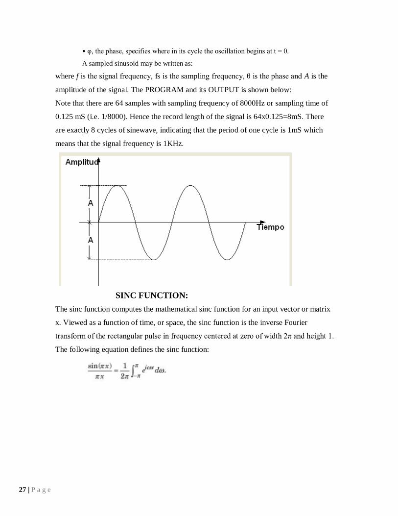
27 | P a g e

• υ, the phase, specifies where in its cycle the oscillation begins at t = 0.

A sampled sinusoid may be written as:

where f is the signal frequency, fs is the sampling frequency, θ is the phase and A is the

amplitude of the signal. The PROGRAM and its OUTPUT is shown below:

Note that there are 64 samples with sampling frequency of 8000Hz or sampling time of

0.125 mS (i.e. 1/8000). Hence the record length of the signal is 64x0.125=8mS. There

are exactly 8 cycles of sinewave, indicating that the period of one cycle is 1mS which

means that the signal frequency is 1KHz.

SINC FUNCTION:

The sinc function computes the mathematical sinc function for an input vector or matrix

x. Viewed as a function of time, or space, the sinc function is the inverse Fourier

transform of the rectangular pulse in frequency centered at zero of width 2π and height 1.

The following equation defines the sinc function:

28 | P a g e

PROGRAM:

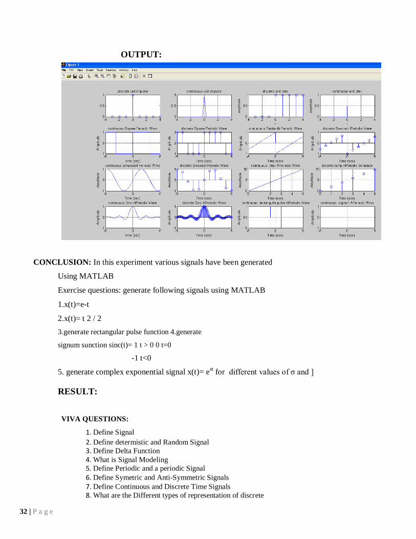
%discrete unit impulse sequence generation clc;

close all; n=-

3:4;

x=[n==0];

subplot(4,4,1),stem(n,x);

title('discrete unit impulse');

%continuous unit impulse signal generation

t=-3:.25:4;

x=[t==0];

subplot(4,4,2),plot(t,x); title('continuous

unit impulse');grid;

% discrete unit step sequence generation

n=-3:4;

y=[n>=0];

subplot(4,4,3),stem(n,y);

xlabel('n')

29 | P a g e

ylabel('amplitude'); title('discrete

unit step');grid;

% continuous unit step signal generation t=-

3:.025:4;

y=[t>=0];

subplot(4,4,4),plot(t,y);

xlabel('t');ylabel('amplitude');title('continuous unit step');grid;

% continuous square wave wave generator

t = -5:.01:5;

x = square(t);

subplot(4,4,5),plot(t,x);

xlabel('Time (sec)');ylabel('Amplitude'); title('continuous Square Periodic Wave');grid;

% discrete square wave wave generator n = -

5:5;

x = square(n);


xlabel('Time (sec)');ylabel('Amplitude');title('discrete Square Periodic Wave');grid;

% continuous sawtooth wave generator t = -

5:.01:5;

x = sawtooth(t);


xlabel('Time (sec)');ylabel('Amplitude'); title('continuous Sawtooth Periodic Wave');grid;

% discrete sawtooth sequence generator

30 | P a g e

n = -5:5;

x = sawtooth(n);


xlabel('Time (sec)');ylabel('Amplitude');title('discrete Sawtooth Periodic Wave');grid;

% continuous sinsodial signal generator t = -

5:.01:5;

x = sin(t);


xlabel('Time (sec)');ylabel('Amplitude'); title('continuous Sinusodial Periodic Wave');grid;

% discrete sinsodial sequence generator n = -

5:5;

x = sin(n);


xlabel('Time (sec)');ylabel('Amplitude');title('discrete Sinsodial Periodic Wave');grid;

% continuous ramp signal generator t =

0:.01:5;

x=2*t;


xlabel('Time (sec)');ylabel('Amplitude'); title('continuous ramp APeriodic Wave');grid;

% discrete ramp sequence generator n =

0:5;

x=2*n;


xlabel('Time (sec)');ylabel('Amplitude');title('discrete ramp APeriodic sequence');grid

31 | P a g e

% continuous sinc signal generator

t = -5:.01:5;

x = sinc(t);


xlabel('Time (sec)');ylabel('Amplitude'); title('continuous Sinc APeriodic Wave');grid;

% discrete sinc sequence generator n = -

5:.1:5;

x = sinc(n);


xlabel('Time (sec)');ylabel('Amplitude');title('discrete Sinc APeriodic Wave');grid;

%To generate a Aperiodic rectangular pulse t=-

5:0.01:5;

pulse = rectpuls(t,2); %pulse of width 2 time units

subplot(4,4,15),plot(t,pulse);

xlabel('Time (sec)');ylabel('Amplitude');title('continuous rectangular pulse APeriodic

Wave');grid;

%To generate a Aperiodic signum function t=-

5:0.01:5;

pulse = sign(t); %pulse of width 2 time units

subplot(4,4,16),plot(t,pulse);

xlabel('Time (sec)');ylabel('Amplitude');title('continuous signum APeriodic Wave');grid;

32 | P a g e

OUTPUT:

CONCLUSION: In this experiment various signals have been generated

Using MATLAB

Exercise questions: generate following signals using MATLAB

1.x(t)=e-t

2.x(t)= t 2 / 2

3.generate rectangular pulse function 4.generate

signum sunction sinc(t)= 1 t > 0 0 t=0

-1 t<0

5. generate complex exponential signal x(t)= est for different values of σ and ]

RESULT:

VIVA QUESTIONS:

1. Define Signal

2. Define determistic and Random Signal

3. Define Delta Function

4. What is Signal Modeling

5. Define Periodic and a periodic Signal

6. Define Symetric and Anti-Symmetric Signals

7. Define Continuous and Discrete Time Signals

8. What are the Different types of representation of discrete

33 | P a g e

EXPERIMENT-3

OPERATIONS ON SIGNALS AND SEQUENCES

AIM: To performs functions on signals and sequences such as addition, multiplication, scaling, shifting, folding, computation of energy and average power.

EQUIPMENT AND SOFTWARE:


MATLAB Software

THEORY:

Basic Operation on Signals:

Time shifting: y(t)=x(t-T)The effect that a time shift has on the appearance of a signal If T is a

positive number, the time shifted signal, x (t -T ) gets shifted to the right, otherwise it gets

shifted left.

Signal Shifting and Delay:

Time reversal: Y(t)=y(-t) Time reversal _ips the signal about t = 0

Signal Addition and Substraction :

Addition: any two signals can be added to form a third signal, z (t) = x

(t) + y (t)

Multiplication/Divition : of two signals, their product is also a signal. z (t) = x

(t) y (t)

ENERGY AND POWER SIGNAL:A signal can be categorized into energy signal or power

signal: An energy signal has a finite energy, 0 < E < ∞. In other words, energy signals have

values only in the limited time duration. For example, a signal having only one square pulse is

energy signal. A signal that decays exponentially has finite energy, so, it is also an energy signal.

The power of an energy signal is 0, because of dividing finite energy by infinite time (or length).

On the contrary, the power signal is not limited in time. It always exists from beginning to end

and it never ends. For example, sine wave in infinite length is power signal. Since the

energy of a power signal is infinite, it has no meaning to us. Thus, we use power

(energy per given time) for power signal, because the power of power signal is finite, 0 <

P < ∞.

34 | P a g e

PROGRAM:

Operations on signals such as addition, subtraction,

multiplication,amplitude scaling

clc;

clear

all;

close

all;

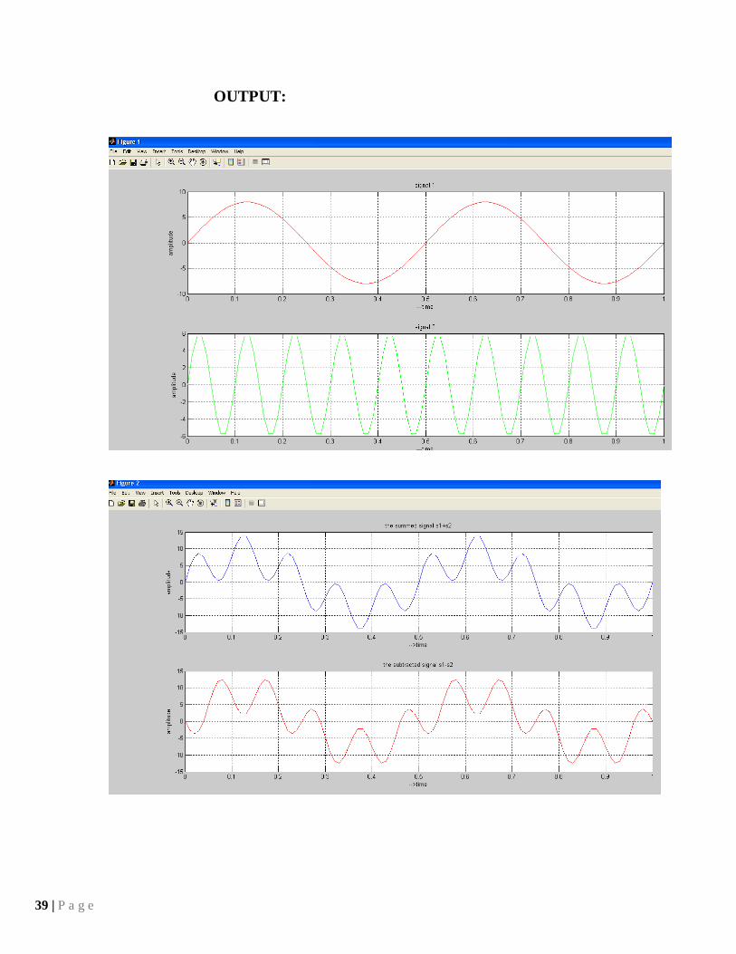
%plot 2 hz sinusodial

signal t=0:.01:1;

f1=2; A=8;

s1=A*sin(2*pi*f1*t);

figure,

subplot(2,1,1),plot(t,s1,'r');

grid; xlabel('---time');

ylabel('amplitude');

title('signal 1');

%plot 10 hz sinusodial

signal t=0:.01:1;

f2=10;

A=6;

s2=A*sin(2*pi*f2*t);

subplot(2,1,2),plot(t,s2,'g');gri

d; xlabel('---time');


title('signal 2');

%signal

y=s1+s2;

figure,

subplot(2,1,1),plot(t,y);gri

d; xlabel('-->time');


35 | P a g e

title('the summed signal s1+s2');

%signal subtraction y=s1-s2;

subplot(2,1,2),plot(t,y,'r');gri

d; xlabel('-->time');


title('the subtracted signal s1-s2');

%signal multiplication element by

element y=s1.*s2;

figure,

plot(t,y,'g')

;

xlabel('-->time');

ylabel('amplitude')

;

title('the multiplied signal s1.*s2');

%Amplitude scaling of signal

s1 alpa= 3;

y=alpha*s1

; figure,

subplot(2,1,1),plot(t,y);

xlabel('-->time');

ylabel('amplitude')

;

title('the signal s1 amplitude is multiplied by alpha');

%amplitude scaling of signal

s2 alpha=1/2;

y=alpha*s2;

subplot(2,1,2),plot(t,y)

;

xlabel('-->time');

ylabel('amplitude')

;

title('the signal s2 is amplitude scaled by 1/alpha');

36 | P a g e

PROGRAM2: Operations on signals such as time shifting, time scaling & time reversal

clc; clear all;

close all;

%plot ramp signal

t=[0:0.01:5];

x=1*t;

subplot(2,2,1),plot(t,x);grid;axis([0 5 0 5]);

title('ramp signal');xlabel('t');ylabel('amplitude');

%plot advanced ramp signal t=[-

3:0.01:2]

x=1*(t+3); subplot(2,2,2),plot(t,x);grid;axis([-3

2 0 5]);

title('advanced ramp signal');xlabel('t');ylabel('amplitude');

%plot delayed ramp signal

t=[3:0.01:8];

x=1*(t-3); subplot(2,2,3),plot(t,x);grid;axis([3

8 0 5]);

title('delayed ramp signal');xlabel('t');ylabel('amplitude');

%plot folding or time reversal operation t=[-

5:.01:0];

x=1*-t;

subplot(2,2,4),plot(t,x);grid;

title('time reversal operation');xlabel('t');ylabel('amplitude');

%plot time scaling t=[-

6:.01:6];

x=2*rectpuls(t,4);

figure;

subplot(3,1,1),plot(t,x);grid;

title('original signal');xlabel('t');ylabel('amplitude');

37 | P a g e

%plot compressed signal t=[-

6:.01:6];

x=2*rectpuls(2*t,4);

subplot(3,1,2),plot(t,x,'g');grid;

title('compressed signal');xlabel('t');ylabel('amplitude');

%plot('expanded signal t=[-

6:.01:6];

x=2*rectpuls(1/2*t,4);

subplot(3,1,3),plot(t,x,'r');grid;

title('expanded signal');xlabel('t');ylabel('amplitude');

PROGRAM3: Operations on sequences

%PROGRAM on operations on sequences clc;

clear all; close

all;

%plot addition sequences

N=input('enter the number of elements');

x1=input('enter the first sequence');

x2=input('enter the second sequence'); n=0:N-

1;

subplot(4,4,1),stem(n,x1);title('first sequence');axis([-3 3 0 10]);grid;

subplot(4,4,2),stem(n,x2);title('second sequence');axis([-3 3 0 10]);grid;

subplot(4,4,3),stem(n,x1+x2);title('additon sequence');axis([0 3 0 15 ]);grid;

subplot(4,4,4),stem(n,x1-x2);title('subtraction sequence');axis([-3 3 -2 5]);grid;

subplot(4,4,5),stem(n,x1.*x2);title('multiplication sequence');axis([-3 3 0 54]);grid;

%amplitude scaling sequence

y=5*x1; subplot(4,4,6),stem(n,y);

title('amplitude scaling sequence');grid;axis([-3 3 0 50]);

%time delay sequence

subplot(4,4,7),stem(n+2,x1);

title('time delayed signal');grid;

38 | P a g e

%time advance sequence

subplot(4,4,8),stem(n-2,x1);grid;

title('time advance sequence');

%time folding sequence;

subplot(4,4,9),stem((-n),x1);

xlabel('n');ylabel('amplitude');grid;

title('time folding sequence');

%time scaling sequence

subplot(4,4,10),stem(2*n,x1);

xlabel('n');ylabel('amplitude');grid;

title('time scaling sequence');

PROGRAM4:energy & power

clc; clear all;

close all;

%energy of a signal N=input('enter

the value of N'); n=-N:N;

x=cos((pi*n)/2);

E=sum(norm(x)^2);

disp('energy is'); disp(E);

%power of a signal

p=E/((2*N)+1);

disp('power is');

disp(p);

39 | P a g e

OUTPUT:

40 | P a g e

PROGRAM2o/p:

41 | P a g e

PROGRAM3 o/p:

enter the number of elements5

enter the first sequence[3 4 7 9 8]

enter the second sequence[1 2 3 4 6]

42 | P a g e

PROGRAM4 o/p:

enter the value of N200

energy is

201

power is 0.5012

CONCLUSION:

In this experiment various oprations on signals and sequences and energyand power of

signals have been calculated Using MATLAB

Exersize questions:

1.x(t)= u(-t+1)

2. x(t)=3r(t-1)

3. x(t)=U(n+2-u(n-3)

4. x(n)=x1(n)+x2(n)where x1(n)={1,3,2,1},x2(n)={1,-2,3,2}

5. x(t)=r(t)-2r(t-1)+r(t-2)

6. x(n)=2δ(n+2)-2δ(n-4), -5≤ n ≥5.

7. X(n)={1,2,3,4,5,6,7,6,5,4,2,1} determine and plot the following sequence

a. x1(n)=2x(n-5-3x(n+4))

1. b. x2(n)=x(3-n)+x(n)x(n-2)

4 calculate the following signals energies

1.x(t)= e j(2t+Π/4)

2.x(t)=cos(t)

3.x(t)=cos(Π/4 n

RESULT:

VIVA QUESTIONS:

1. What are the Different types of Operation performed on signals.

2. Define Energy and Power signal.

3. What is the result of adding & subtracting two unit step signals.

4. Consider any one signal and perform shifting, scaling and reversal operations

5. Define the Properties of Impulse Signal

6. What is Causality Condition of the Signal

43 | P a g e

EXPERIMENT-4

GIBBS PHENOMENON

AIM: To verify the Gibbs Phenomenon.

EQUIPMENTS:


MATLAB Software

THEORY:

the Gibbs phenomenon, the Fourier series of a piecewise continuously differentiable periodic

function behaves at a jump discontinuity.the n the approximated function shows amounts of ripples at

the points of discontinuity. This is known as the Gibbs Phenomina . partial sum of the Fourier series

has large oscillations near the jump, which might increase the maximum of the partial sum above that

of the function itself. The overshoot does not die out as the frequency increases, but approaches a

finite limit

The Gibbs phenomenon involves both the fact that Fourier sums overshoot at a jump discontinuity,

and that this overshoot does not die out as the frequency increases Gibbs Phenomina

PROGRAM :

t=0:0.1:(pi*8);

y=sin(t);

subplot(5,1,1);

plot(t,y);

xlabel('k'); ylabel('amplitude');

title('gibbs phenomenon'); h=2;

%k=3;

for k=3:2:9

y=y+sin(k*t)/k;

subplot(5,1,h);

44 | P a g e

plot(t,y);

xlabel('k');


h=h+1;

end

OUTPUT:

45 | P a g e

CONCLUSION:

In this experiment Gibbs phenomenon have been demonstrated

Using MATLAB

RESULT:

VIVA QUESTIONS:

1. State Gibbs phenomenon

46 | P a g e

EXPERIMENT-5

Fourier Transform AND INVERSE FOURIER TRANSFORM

AIM: To find the Fourier Transform of a given signal and plotting its magnitude and

phase spectrum

EQUIPMENTS:


MATLAB Software.

THEORY:

Fourier Transform Theorems:

We may use Fourier series to motivate the Fourier transform as follows. Suppose that ƒ

Is a function which is zero outside of some interval [−L/2, L/2]. Then for any T ≥ L we may expand

ƒ in a Fourier series on the interval [−T/2,T/2], where the "amount" of the wave e 2πinx/T in the

Fourier series of ƒ is given by By definition

DFT of a sequence

Where N= Length of sequence. K=

Frequency Coefficient.

n = Samples in time domain. FFT : -

47 | P a g e

Fast Fourier transformer . There are

Two methods.

1. Decimation in time (DIT FFT).

2. Decimation in Frequency (DIF FFT).

PROGRAM:

clc; close all;

clear all;

x=input('enter the sequence');

N=length(x);

n=0:1:N-1;

y=fft(x,N)

subplot(2,1,1);

stem(n,x);

title('input sequence');

xlabel('time index n----->');

ylabel('amplitude x[n]----> ');

subplot(2,1,2);

stem(n,y);

title('OUTPUT sequence'); xlabel('

Frequency index K---->');

ylabel('amplitude X[k]------>');

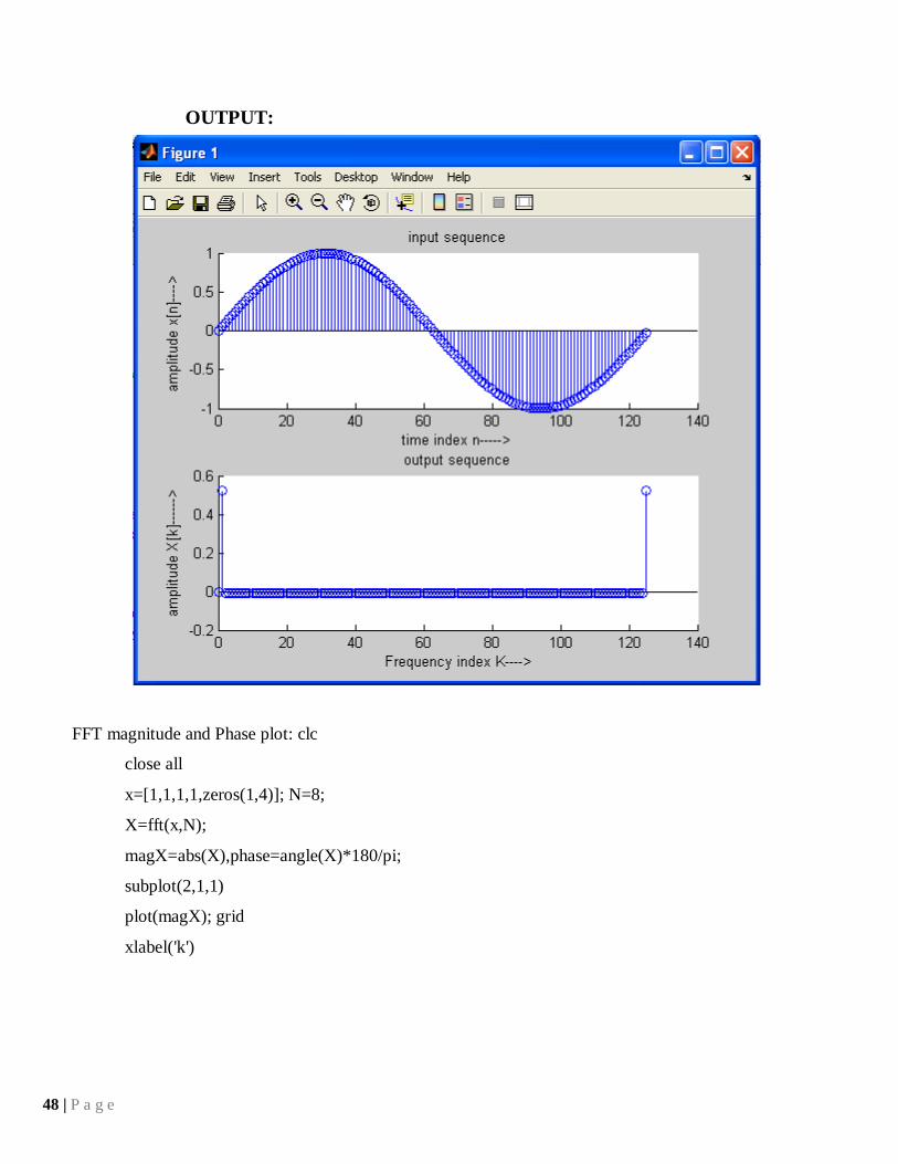
48 | P a g e

OUTPUT:

FFT magnitude and Phase plot: clc

close all

x=[1,1,1,1,zeros(1,4)]; N=8;

X=fft(x,N);

magX=abs(X),phase=angle(X)*180/pi;

subplot(2,1,1)

plot(magX); grid

xlabel('k')

49 | P a g e

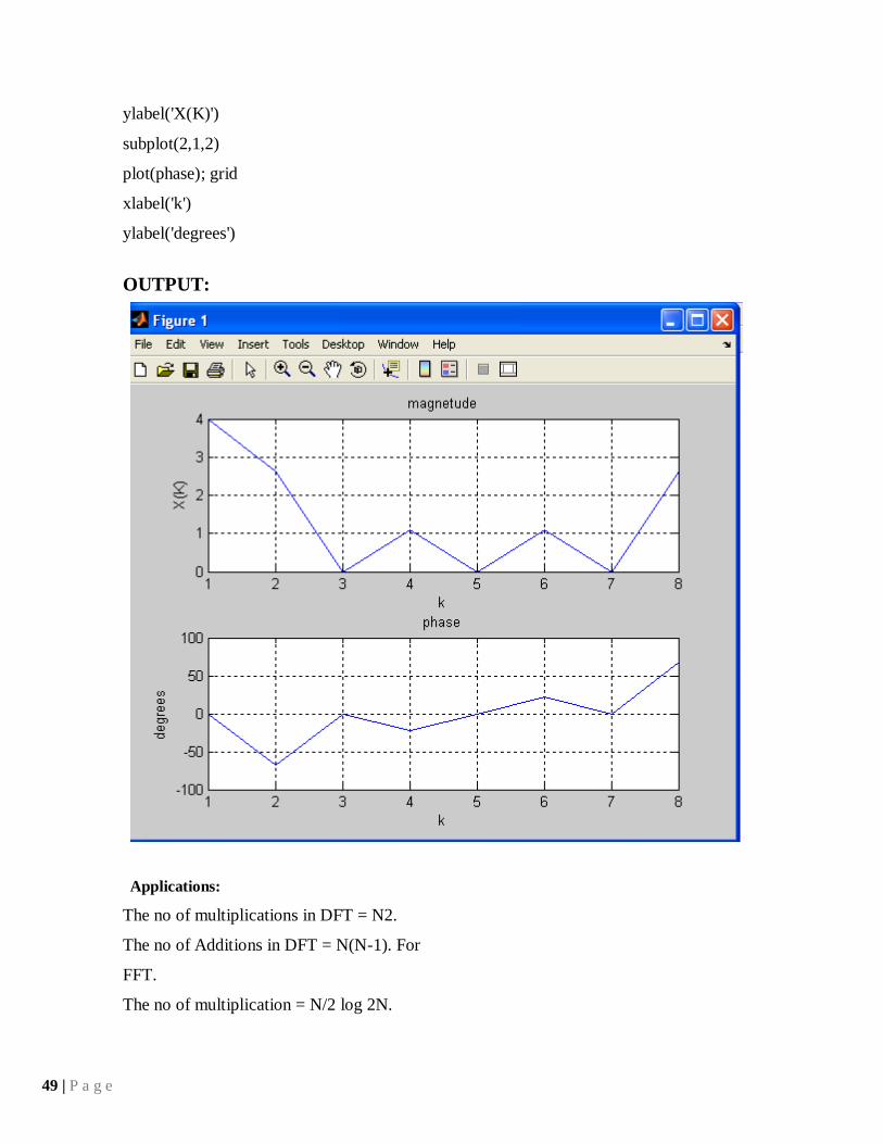
ylabel('X(K)')

subplot(2,1,2)

plot(phase); grid

xlabel('k')

ylabel('degrees')

OUTPUT:

Applications:

The no of multiplications in DFT = N2.

The no of Additions in DFT = N(N-1). For

FFT.

The no of multiplication = N/2 log 2N.

50 | P a g e

The no of additions = N log2 N.

CONCLUSION:

In this experiment the fourier transform of a given signal and plotting

its magnitude and phase spectrum have been demonstrated using matlab

RESULT:

VIVA QUESTIONS:

1 .Define Fourier Series

2 What is Half Wave Symmetry

3 What are the properties of Continuous-Time Fourier Series

4 Define Fourier Transform

51 | P a g e

EXPERIMENT-6

PROPERTIES OF FOURIER TRNASFORM

AIM:

To verify thE properties of DTFT of a given discrete-time signal

EQUIPMENTS:


MATLAB Software

THEORY:

We will represent the spectrum of DTFT by X(ejw

)

DTFT Properties

Time shifting

Time reversal

Convolution

Let x[n] X(ejw

) and h[n] H(ejw

).

If y[n] = x[n] h[n], then Y(e

jw) = X(e

jw)H(e

jw)

52 | P a g e

PROGRAM:

% Time-Shifting Property of DTFT

clc;

clear all;

close all;

w = -pi:2*pi/255:pi; wo = 0.4*pi; D = 10;

num = [1 2 3 4 5 6 7 8 9];

h1 = freqz(num, 1, w);

h2 = freqz([zeros(1,D) num], 1, w);

subplot(2,2,1)

plot(w/pi,abs(h1));grid

title('Magnitude Spectrum of Original Sequence')

subplot(2,2,2)


title('Magnitude Spectrum of Time-Shifted Sequence')

subplot(2,2,3)

plot(w/pi,angle(h1));grid

title('Phase Spectrum of Original Sequence')

subplot(2,2,4)


title('Phase Spectrum of Time-Shifted Sequence')

w = -pi:2*pi/255:pi; wo = 0.4*pi; D = 10;

num = [1 2 3 4 5 6 7 8 9];


h2 = freqz([zeros(1,D) num], 1, w);

subplot(2,2,1)



subplot(2,2,2)


title('Magnitude Spectrum of Time-Shifted Sequence')

subplot(2,2,3)



53 | P a g e

subplot(2,2,4)


title('Phase Spectrum of Time-Shifted Sequence')

OUTPUT:

% Time-Reversal Property of DTFT

clc;

clear all;

close all;

w = -pi:2*pi/255:pi;

num = [1 2 3 4];

L = length(num)-1;


h2 = freqz(fliplr(num), 1, w);

h3 = exp(w*L*i).*h2;

subplot(2,2,1)


54 | P a g e


subplot(2,2,2)


title('Magnitude Spectrum of Time-Reversed Sequence')

subplot(2,2,3)



subplot(2,2,4)


title('Phase Spectrum of Time-Reversed Sequence')

OUTPUT:

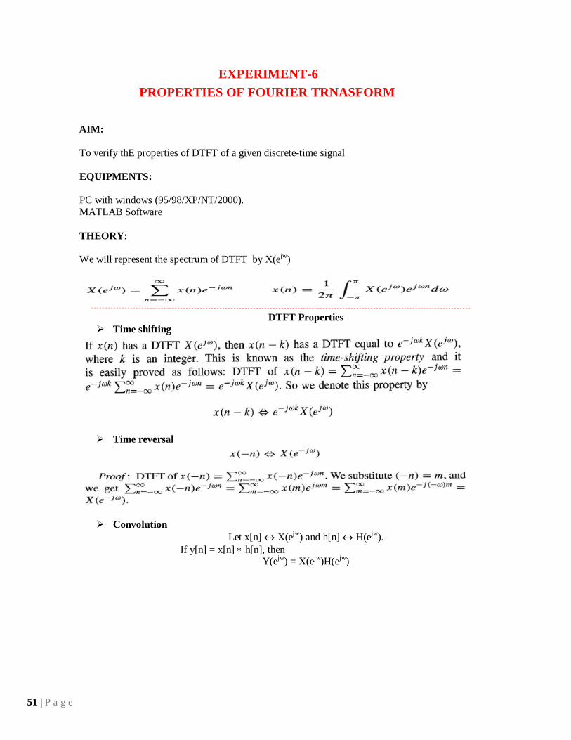
% Convolution Property of DTFT

clc;

clear all;

close all;

w = -pi:2*pi/255:pi;

55 | P a g e

x1 = [1 3 5 7 9 11 13 15 17];

x2 = [1 -2 3 -2 1];

y = conv(x1,x2);

h1 = freqz(x1, 1, w);

h2 = freqz(x2, 1, w);

hp = h1.*h2;

h3 = freqz(y,1,w);

subplot(2,2,1)

plot(w/pi,abs(hp));grid

title('Product of Magnitude Spectra')

subplot(2,2,2)


title('Magnitude Spectrum of Convolved Sequence')

subplot(2,2,3)

plot(w/pi,angle(hp));grid

title('Sum of Phase Spectra')

subplot(2,2,4)


title('Phase Spectrum of Convolved Sequence')

OUTPUT:

56 | P a g e

CONCLUSION: In this experiment the properties of DTFT are verified using MATLAB

RESULT:

PRE LAB QUESTIONS

1.Define DTFT

2.What is the convolution theorem of DTFT ?

3. What is the time shifting property of DTFT ?

4. State the Time-reversal property of DTFT.

57 | P a g e

LAB ASSIGNMENT

1. To verify the frequency-shifting property of the DTFT

POST LAB QUESTIONS

1. What is effect of time shifting property of DTFT?

2. What is effect of time reversal property of DTFT?

3. State the convolution property of DTFT.

58 | P a g e

EXPERIMENT-7

LAPLACE TRNASFORM

AIM: To perform waveform synthesis using Laplace Transform of a given signal

EQUIPMENTS:


MATLAB Software

THEORY:

Bilateral Laplace transform :

When one says "the Laplace transform" without qualification, the unilateral or one- sided

transform is normally intended. The Laplace transform can be alternatively defined as the

bilateral Laplace transform or two-sided Laplace transform by extending the limits of

integration to be the entire real axis. If that is done the common unilateral transform

simply becomes a special case of the bilateral transform where the definition of the

function being transformed is multiplied by the Heaviside step function.

The bilateral Laplace transform is defined as follows:

The inverse Laplace transform is given by the following complex integral, which

is known by various names (the Bromwich integral, the Fourier-Mellin integral,

and

Mellin's inverse formula):

PROGRAM:

syms f t; f=t;

laplace(f)

PROGRAM for nverse Laplace Transform

f(s)=24/s(s+8) invese LT

syms F s

59 | P a g e

F=24/(s*(s+8));

ilaplace(F)

y(s)=24/s(s+8) invese LT poles and zeros

Signal synthese using Laplace Tnasform:

clear all

clc t=0:1:5

s=(t); subplot(2,3,1)

plot(t,s); u=ones(1,6)

subplot(2,3,2)

plot(t,u); f1=t.*u;

subplot(2,3,3)

plot(f1);

s2=-2*(t-1);

subplot(2,3,4);

plot(s2);

u1=[0 1 1 1 1 1];

f2=-2*(t-1).*u1;

subplot(2,3,5);

plot(f2);

u2=[0 0 1 1 1 1];

f3=(t-2).*u2;

subplot(2,3,6);

plot(f3); f=f1+f2+f3;

figure; plot(t,f);

% n=exp(-t);

% n=uint8(n);

60 | P a g e

% f=uint8(f);

% R = int(f,n,0,6)

laplace(f);

OUTPUT:

61 | P a g e

CONCLUSION:

In this experiment the Triangular signal synthesised using

Laplece Trnasforms using MATLAB

Applications of laplace transforms:

1.Derive the circuit (differential) equations in the time domain, then transform these ODEs to

the s-domain;

2.Transform the circuit to the s-domain, then derive the circuit equations in the sdomain

(using the concept of "impedance").

The main idea behind the Laplace Transformation is that we can solve an equation

(or system of equations) containing differential and integral terms by transforming

the equation in "t-space" to one in "s-space". This makes the problem much easier to

solve.

RESULT:

VIVA QUESTIONS:

1. Define Laplace-Transform

2. What is the Condition for Convergence of the L.T

3. What is the Region of Convergence(ROC)

4. State the Shifting property of L.T

5. State convolution Property of L.T

6. Define Transfer Function

7. Define Pole-Zeros of the Transfer Function

62 | P a g e

EXPERIMENT-8

Z- TRANSFORMS

AIM: To locating the zeros and poles and plotting the pole zero maps in s-plane

and Zplane for the given transfer function

EQUIPMENTS:


MATLAB Software

THEORY:

Z-transforms

the Z-transform converts a discrete time-domain signal, which is a sequence of real or

complex numbers, into a complex frequency-domain representation.The Z-transform,

like

many other integral transforms, can be defined as either a one-sided or two-sided

transform.

Bilateral Z-transform

The bilateral or two-sided Z-transform of a discrete-time signal x[n] is the function X(z)

defined as

Unilateral Z-transform

Alternatively, in cases where x[n] is defined only for n ≥ 0, the single-sided or unilateral

Z-transform is defined as

In signal processing, this definition is used when the signal is causal.

63 | P a g e

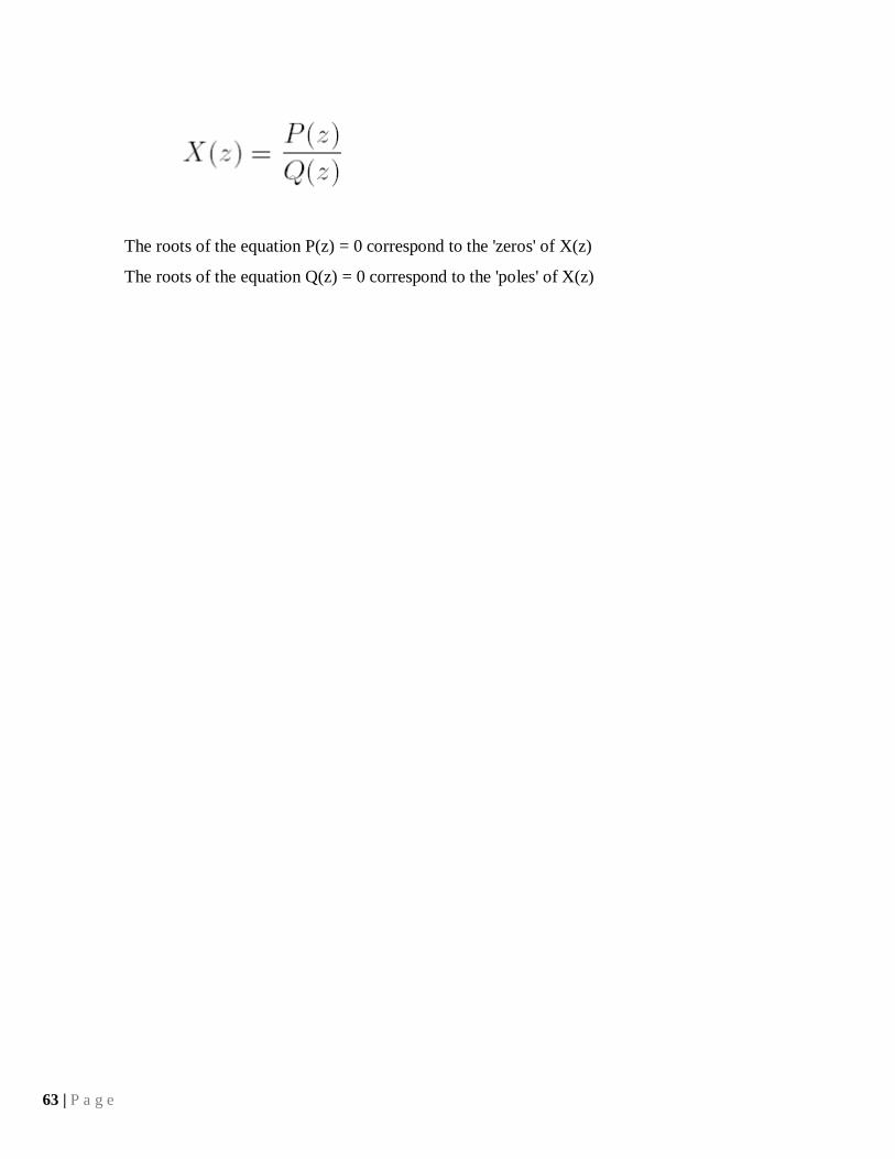
The roots of the equation P(z) = 0 correspond to the 'zeros' of X(z)

The roots of the equation Q(z) = 0 correspond to the 'poles' of X(z)

64 | P a g e

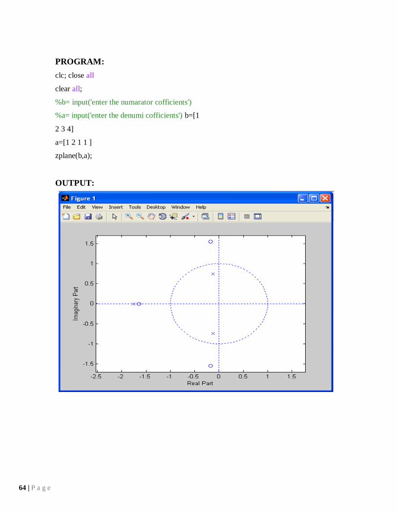
PROGRAM:

clc; close all

clear all;

%b= input('enter the numarator cofficients')

%a= input('enter the denumi cofficients') b=[1

2 3 4]

a=[1 2 1 1 ]

zplane(b,a);

OUTPUT:

65 | P a g e

CONCLUSION:

In this experiment the zeros and poles and plotting the pole zero maps in s-plane and z-

plane for the given transfer function using MATLAB.

RESULT:

VIVA QUESTIONS:

1. What is the Relationship between L.T & F.T &Z.T

2. Fined the Z.T of a Impulse and step

3. What are the Different Methods of evaluating inverse z-T

4. Explain Time-Shifting property of a Z.T

5. what are the ROC properties of a Z.T

6. Define Initial Value Theorem of a Z.T

7. Define Final Value Theorem of a Z.T

66 | P a g e

A

I

M

EXEXPERIMENT-9

CONVOLUTION BETWEEN SIGNALS AND SEQUENCE

AIM;To find the output with linear convolution operation Using MATLAB

Software.

EQUIPMENTS:


MATLAB Software

THEORY:

Linear Convolution involves the following operations.

1. Folding

2. Multiplication

3. Addition

4. Shifting

These operations can be represented by a Mathematical Expression as follows:

PROGRAM:

clc; close all;

clear all;

x=input('enter input sequence');

h=input('enter impulse response');

y=conv(x,h);

subplot(3,1,1);

stem(x);

xlabel('n');ylabel('x(n)');

67 | P a g e

title('input signal') subplot(3,1,2); stem(h);

xlabel('n');ylabel('h(n)');

title('impulse response')

subplot(3,1,3);

stem(y); xlabel('n');ylabel('y(n)');

title('linear convolution') disp('The

resultant signal is'); disp(y)

linear convolution

INTPUT:

enter input sequence[1 4 3 2]

enter impulse response[1 0 2 1] The

resultant signal is

1 4 5 11 10 7 2

OUTPUT:

68 | P a g e

CONCLUSION:

In this experiment convolution of various signals have been

performed Using MATLAB

Applications:

Convolution is used to obtain the response of an LTI system to an arbitrary input

signal.It

is used to find the filter response and finds application in speech processing and radar

signal processing.

Excersize questions: perform convolution between the following signals 1.

X(n)=[1 -1 4 ], h(n) = [ -1 2 -3 1]

2. perform convolution between the. Two periodic sequences

x1(t)=e-3t{u(t)-u(t-2)} , x2(t)= e -3t for 0 ≤ t ≤ 2

RESULT:

VIVA QUESTIONS:

1. Define Convolution

2. Define Properties of Convolution

69 | P a g e

EXPERIMENT-10

AUTO CORRELATION AND CROSS CORRELATION BETWEEN

SIGNALS AND SEQUENCES

AIM:To compute auto correlation and cross correlation between signals and sequences

EQUIPMENTS:


MATLAB Software

THEORY:

Correlations of sequences:

It is a measure of the degree to which two sequences are similar. Given two real valued

Sequences x(n) and y(n) of finite energy,

Convolution involves the following operations.

1. Shifting

2. Multiplication

3. Addition

These operations can be represented by a Mathematical Expression as follows:

Cross correlation

The index l is called the shift or lag parameter

Autocorrelation

The special case: y(n)=x(n)

PROGRAM:

% Cross Correlation

clc;

close all;

70 | P a g e

clear all;

x=input('enter input sequence');

h=input('enter the impulse suquence');

subplot(3,1,1);

stem(x);

xlabel('n');

ylabel('x(n)'); title('input

signal'); subplot(3,1,2);

stem(h); xlabel('n');

ylabel('h(n)'); title('impulse

signal'); y=xcorr(x,h);

subplot(3,1,3);

stem(y); xlabel('n');

ylabel('y(n)');

disp('the resultant signal is');

disp(y);

title('correlation signal');

OUTPUT:

71 | P a g e

PROGRAM:

% auto correlation clc;

close all; clear

all;

x = [1,2,3,4,5]; y = [4,1,5,2,6];

subplot(3,1,1);

stem(x); xlabel('n');

ylabel('x(n)'); title('input

signal'); subplot(3,1,2);

stem(y); xlabel('n');

ylabel('y(n)'); title('input

signal'); z=xcorr(x,x);

subplot(3,1,3);

stem(z); xlabel('n');

ylabel('z(n)');

title('resultant signal signal');

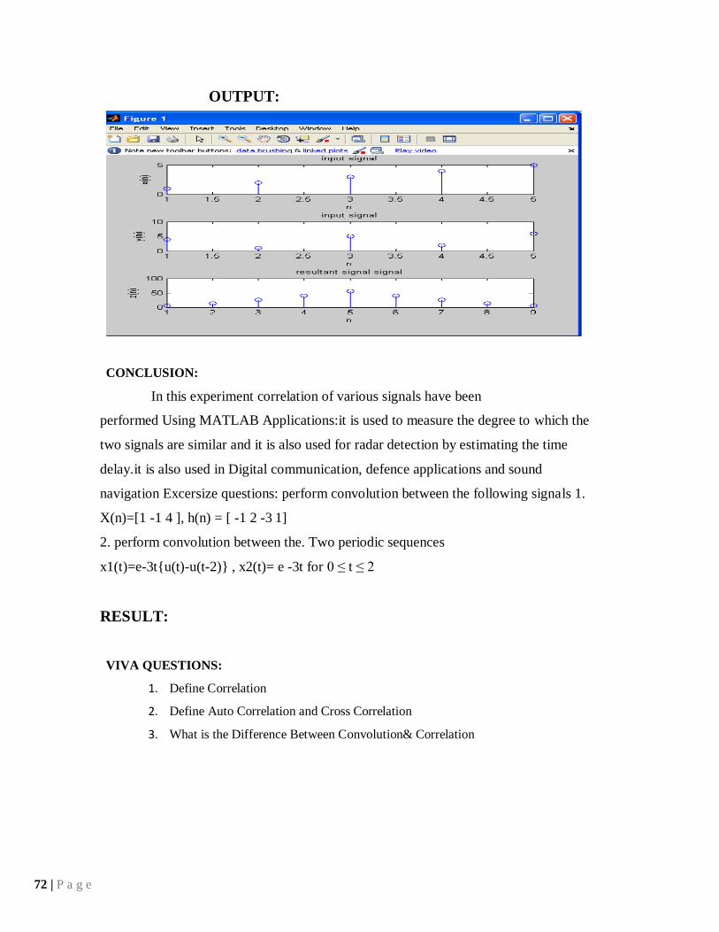
72 | P a g e

OUTPUT:

CONCLUSION:

In this experiment correlation of various signals have been

performed Using MATLAB Applications:it is used to measure the degree to which the

two signals are similar and it is also used for radar detection by estimating the time

delay.it is also used in Digital communication, defence applications and sound

navigation Excersize questions: perform convolution between the following signals 1.

X(n)=[1 -1 4 ], h(n) = [ -1 2 -3 1]

2. perform convolution between the. Two periodic sequences

x1(t)=e-3t{u(t)-u(t-2)} , x2(t)= e -3t for 0 ≤ t ≤ 2

RESULT:

VIVA QUESTIONS:

1. Define Correlation

2. Define Auto Correlation and Cross Correlation

3. What is the Difference Between Convolution& Correlation

73 | P a g e

EXPERIMENT-11

Gaussian Noise

AIM: To Verify the Gaussian noise.

EQUIPMENTS:


MATLAB Software

PROGRAM:

clc; clear all;

close all;

%% Defining the range for the Random variable

dx=0.01; %delta x

x=-3:dx:3;

[m,n]=size(x);

%% Defining the parameters of the pdf

mu_x=0; % mu_x=input('Enter the value of mean');

sig_x=0.1; % sig_x=input('Enter the value of varience');

%% Computing the probability density function

px1=[];

a=1/(sqrt(2*pi)*sig_x); for

j=1:n

px1(j)=a*exp([-((x(j)-mu_x)/sig_x)^2]/2);

end

%% Computing the cumulative distribution function

cum_Px(1)=0;

for j=2:n

cum_Px(j)=cum_Px(j-1)+dx*px1(j);

end

%% Plotting the results

figure(1)

74 | P a g e

plot(x,px1);grid

axis([-3 3 0 1]);

title(['Gaussian pdf for mu_x=0 and sigma_x=', num2str(sig_x)]);

xlabel('--> x')

ylabel('--> pdf') figure(2)

plot(x,cum_Px);grid

axis([-3 3 0 1]);

title(['Gaussian Probability Distribution Function for mu_x=0 and sigma_x=',

num2str(sig_x)]);

title('\ite^{\omega\tau} = cos(\omega\tau) + isin(\omega\tau)')

xlabel('--> x')

ylabel('--> PDF')

OUTPUT:

75 | P a g e

RESULT:

76 | P a g e

EXPERIMENT-12

WIENER–KHINCHIN RELATION

AIM: Verification of wiener–khinchine relation

EQUIPMENTS:


MATLAB Software

THEORY:

The Wiener–Khinchin theorem (also known as the Wiener–Khintchine theorem

and sometimes as the Wiener–Khinchin–Einstein theorem or the Khinchin–Kolmogorov

theorem) states that the power spectral density of a wide-sense-stationary random process is

the Fourier transform of the corresponding autocorrelation function.

Continuous case:

Where

is the autocorrelation function defined in terms of statistical expectation, and where is

the power spectral density of the function . Note that the autocorrelation function is

defined in terms of the expected value of a product, and that the Fourier transform of

does not exist in general, because stationary random functions are not square integrable.

The asterisk denotes complex conjugate, and can be omitted if the random process is

realvalued.

Discrete case:

Where

77 | P a g e

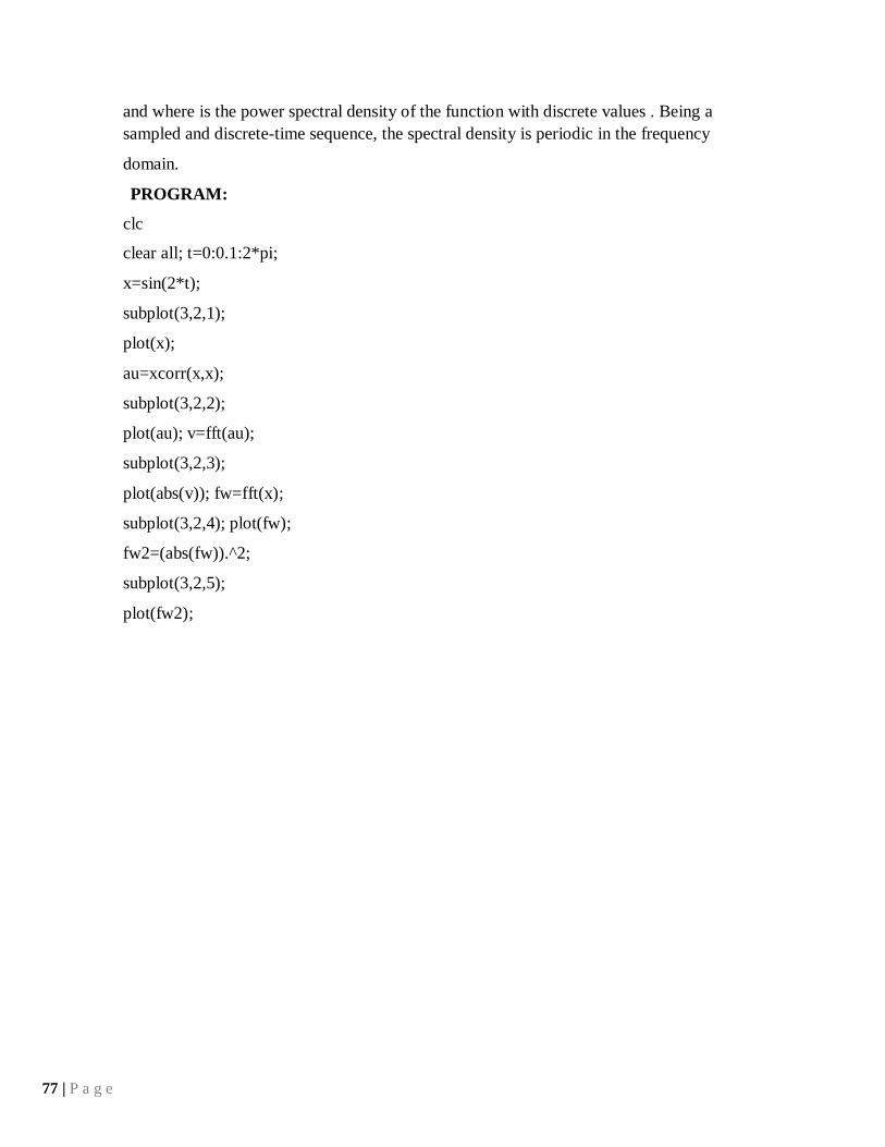
and where is the power spectral density of the function with discrete values . Being a

sampled and discrete-time sequence, the spectral density is periodic in the frequency

domain.

PROGRAM:

clc

clear all; t=0:0.1:2*pi;

x=sin(2*t);

subplot(3,2,1);

plot(x);

au=xcorr(x,x);

subplot(3,2,2);

plot(au); v=fft(au);

subplot(3,2,3);

plot(abs(v)); fw=fft(x);

subplot(3,2,4); plot(fw);

fw2=(abs(fw)).^2;

subplot(3,2,5);

plot(fw2);

78 | P a g e

RESULT:

VIVA QUESTIONS:

1. State wiener-kinchen relationship

79 | P a g e

EXPERIMENT NO: 13

DISTRIBUTION AND DENSITY FUNCTIONS OF STANDARD

RANDOM VARIABLES

AIM: To calculate PDF and CDF of standard random variables

EQUIPMENTS:


MATLAB Software

THEORY:

Uniform Random Variable

pdf is constant over the (a,b) interval and CDF is the ramp function in

the same interval

Exponential Random Variable

Mathematically (pdf and CDF, respectively)

Rayleigh Random Variable

The probability density function of the Rayleigh distribution is

https://en.wikipedia.org/wiki/Probability_density_function

80 | P a g e

where σ is the scale parameter of the distribution. The cumulative distribution function is

For

PROGRAM:

%Distribution and density functions of standard random variables clc;

clear all;

close all;

x=-5:0.01:5;

% uniform random variable

a=2;b=3;

%PDF

f=(1/(b-a)).*(x>=a).*(x<=b);

subplot(3,2,1);

plot(x,f);

%CDF

F=(0*(x<a))+(((x-a)/(b-a)).*(x>=a).*(x<=b))+(1*(x>b));

subplot(3,2,2);

plot(x,F);

% exponential random variable

f=(a.*(exp(-a*x)).*(x>=0))+(0*(x<0));

subplot(3,2,3);

plot(x,f);

%CDF

F=((1-exp(-a*x)).*(x>=0))+(0*(x<0));

subplot(3,2,4);

plot(x,F);

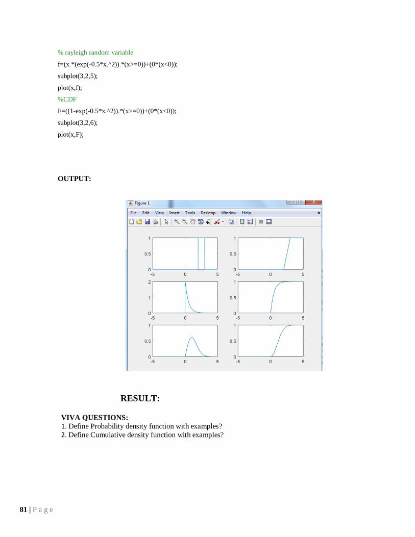
https://en.wikipedia.org/wiki/Scale_parameter

https://en.wikipedia.org/wiki/Cumulative_distribution_function

81 | P a g e

% rayleigh random variable

f=(x.*(exp(-0.5*x.^2)).*(x>=0))+(0*(x<0));

subplot(3,2,5);

plot(x,f);

%CDF

F=((1-exp(-0.5*x.^2)).*(x>=0))+(0*(x<0));

subplot(3,2,6);

plot(x,F);

OUTPUT:

RESULT:

VIVA QUESTIONS:

1. Define Probability density function with examples?

2. Define Cumulative density function with examples?

82 | P a g e

AIM:

EXPERIMENT NO:14

WIDE SENSOR STATIONARY PROCESS

Checking a random process for stationarity in wide sense.

EQUIPMENTS:


MATLAB Software

THEORY:

a stationary process (or strict(ly) stationary process or strong(ly) stationary process)

is a stochastic process whose joint probability distribution does not change when shifted in

time or space. As a result, parameters such as the mean and variance, if they exist, also do

not change over time or position..

Definition

Formally, let Xt be a stochastic process and letrepresent the cumulative distribution

function of the joint distribution of Xt at times t1…..tk. Then, Xt is said to be stationary

if, for all k, for all τ, and for all t1…..tk

Weak or wide-sense stationarity

A weaker form of stationarity commonly employed in signal processing is known as

weak-sense stationarity, wide-sense stationarity (WSS) or covariance stationarity.

WSS random processes only require that 1st and 2nd moments do not vary with respect

to time. Any strictly stationary process which has a mean and a covariance is also WSS.

So, a continuous-time random process x(t) which is WSS has the following restrictions

on its mean function

and autocorrelation function

83 | P a g e

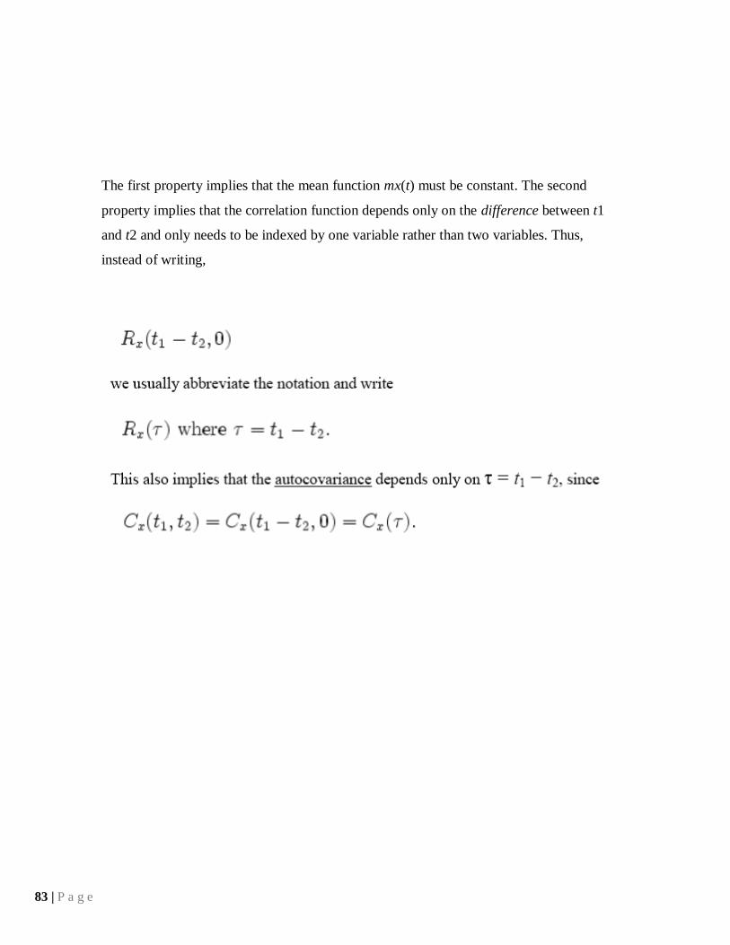
The first property implies that the mean function mx(t) must be constant. The second

property implies that the correlation function depends only on the difference between t1

and t2 and only needs to be indexed by one variable rather than two variables. Thus,

instead of writing,

84 | P a g e

When processing WSS random signals with linear, time-invariant (LTI) filters, it is

helpful to think of the correlation function as a linear operator. Since it is a circulant

operator (depends only on the difference between the two arguments), its eigenfunctions

are the Fourier complex exponentials. Additionally, since the eigenfunctions of LTI

operators are also complex exponentials, LTI processing of WSS random signals is highly

tractable—all computations can be performed in the frequency domain. Thus, the WSS

assumption is widely employed in signal processing algorithms.

Applications:

Stationary is used as a tool in time series analysis, where the raw data are often

transformed to become stationary, for example, economic data are often seasonal and/or

dependent on the price level. Processes are described as trend stationary if they are a

linear combination of a stationary process and one or more processes exhibiting a trend.

Transforming these data to leave a stationary data set for analysis is referred to as de-

trending

Stationary and Non Stationary Random Process:

A random X(t) is stationary if its statistical properties are unchanged by a time shift in the

time origin.When the auto-Correlation function Rx(t,t+T) of the random X(t) varies with

time difference T and the mean value of the random variable X(t1) is independent of the

choice of t1,then X(t) is said to be stationary in the wide-sense or wide-sense stationary .

So a continous- Time random process X(t) which is WSS has the following properties

85 | P a g e

1) E[X(t)]=μX(t)= μX(t+T)

2) The Autocorrelation function is written as a function of T that is

3) RX(t,t+T)=Rx(T)

If the statistical properties like mean value or moments depends on time then the

random process is said to be non-stationary.

When dealing wih two random process X(t) and Y(t), we say that they are jointly

wide-sense stationary if each pocess is stationary in the wide-sense.

Rxy(t,t+T)=E[X(t)Y(t+T)]=Rxy(T).

PROGRAM:

clear all clc

y = randn([1 40])

my=round(mean(y));

z=randn([1 40])

mz=round(mean(z));

vy=round(var(y));

vz=round(var(z));

t = sym('t','real'); h0=3;

x=y.*sin(h0*t)+z.*cos(h0*t);

mx=round(mean(x));

k=2;

xk=y.*sin(h0*(t+k))+z.*cos(h0*(t+k));

x1=sin(h0*t)*sin(h0*(t+k));

x2=cos(h0*t)*cos(h0*(t+k));

c=vy*x1+vz*x1;

%if we solve "c=2*sin(3*t)*sin(3*t+6)" we get c=2cos(6)

%which is a costant does not dependent on variable 't'

% so it is widesence stationary

86 | P a g e

RESULT:

79 | P a g e

signals and systems laboratory

Documents