open quantum dots: physics of the non-hermitian...

Fortschr. Phys. 61, No. 2 – 3, 291 – 304 (2013) / DOI 10.1002/prop.201200065

Open quantum dots:Physics of the non-Hermitian Hamiltonian

D. K. Ferry1,∗, R. Akis1, A. M. Burke1,5, I. Knezevic2, R. Brunner3, R. Meisels3, F. Kuchar3,and J. P. Bird4

1 School of Electrical, Computer, and Energy Engineering, Arizona State University,Tempe AZ 85287-5706, USA

2 Department of Electrical Engineering, University of Wisconsin, Madison WI 53706, USA3 Institut fur Physik, Montanuniversitat Leoben, 8700 Leoben, Austria4 Department of Electrical Engineering, University at Buffalo, Buffalo, NY 14260, USA5 School of Physics, The University of New South Wales, Sydney, Australia

Received 31 March 2012, revised 31 March 2012, accepted 16 April 2012Published online 9 May 2012

Key words Semiconductor quantum dots, classical to quantum transition, projection algebra, dissipation.

Quantum dots provide a natural system in which to study both classical and quantum features of transport,as they possess a very rich set of eigenstates.When coupled to the environment through a pair of quantumpoint contacts, these dots possess a mixed phase space which yields families of closed, regular orbits as wellas an expansive sea of chaos. In this latter case, many of the eigenstates are decohered through interactionwith the environment, but many survive and are referred to as the set of pointer states. These latter states aredescribed by a projected, non-Hermitian Hamiltonian which describes their dissipation through many-bodyinteractions with particles in the external environment.

© 2013 WILEY-VCH Verlag GmbH & Co. KGaA, Weinheim

1 Introduction

Since the beginning of quantum mechanics, the measurement of open quantum systems has been of greatinterest. The earliest papers addressed directly results of measurements. Indeed, measurements have alwaysbeen considered to be classical, as the results appear in the laboratory. But, to make the measurement, thequantum system must be opened so that it can communicate with the external environment in which themeasurement is made. While this is an exceedingly broad topic, measurements on open quantum dots haveshown to be an interesting window onto the general measurement problem for quantum systems and howthe quantum nature evolves into the classical nature [1]. The subject of quantum dots itself is a quite broadtopic [2]. Our interest is in quantum dots formed by electrostatic gates on the surface of a heterostructure,such as GaAs/AlGaAs, in which a two-dimensional electron gas resides at the interface [3], or in similardots defined by in-plane gates.

Early measurements of such open quantum dots clearly exhibited conductance fluctuations, presumablydue to interference effects within these dots [4–9]. These experiments were often interpreted in terms ofan earlier theory which suggested that these fluctuations were due to chaotic behavior, with the quantumtransport being determined from knowledge of the irregular classical scattering dynamics of the samestructures [10, 11]. In such a picture, the quantum mechanics would be completely washed out in theopen quantum dot. Later studies, however, showed that the quantum properties were not washed out, butremained robust within the dot, and that scarred wave functions appeared with regular periodic energy

∗ Corresponding author E-mail: [email protected]

© 2013 WILEY-VCH Verlag GmbH & Co. KGaA, Weinheim

292 D. K. Ferry et al.: Open quantum dots: Physics of the non-Hermitian Hamiltonian

eigenstates [12], and that this behavior would persist irrespective of whether the structure were classicallyregular or chaotic [13].

So, quantum states persist in the open quantum dots and wave function scars are stable, both of whichcould be observed in the oscillatory magneto-conductance of these dots. Which brings us back to the mea-surement problem. In these dots, as well as in quantum information and computation, the border where thetwo worlds of classical and quantum mechanics meet is of great relevance due to the problem of measure-ment. To this discussion, Zurek brought the decoherence theory [14], in which he used the ansatz that, in anopen system, the environment imposes so-called superselection rules by preserving part of the informationthat resides in the classical correlations between the system and the measuring apparatus, leading to anenvironment-induced process of superselection (einselection) [14]. This means that essentially preferredstates (which are termed pointer states) survive the decoherence process related to the coupling with theenvironment. The promotion of certain information, which couples throughout the spectrum of states, ina quantum system due to a natural selection process is known as Quantum Darwinism [15, 16]. QuantumDarwinism is based on the Darwinian concept [17] for the rules of reproduction, heredity, and variation.The pointer states are not only characterized by their robustness, despite the existing environment, but alsoby their ability to create “offspring” of the states which means they advertise the information about them-selves throughout the spectrum. This ability makes it possible for different observers to measure the sameinformation. This connects clearly to results obtained from the classical states. That is, in order to measurea quantum system objectively, one has to design a system where the transition between the classical andquantum world is observable.

From this description, open quantum dots offer a unique window on such behavior as they exhibit amixed classical phase space [18]. Quantum states within these structures that couple well to the outsideenvironment, through the QPC’s confining constrictions, are heavily decohered. These states give rise tothe chaotic sea [19] that exists in the classical phase space of the dot. Other states within the cavity remainrobust throughout this decoherence process, since they do not couple to the leads, and are the pointerstates [14,20].This provides a natural connection between the quantum and the classical system, and allowsone to study the transition from one to the other [21, 22].

The pointer states represent a subset of the total set of states in the coupled dot plus environment system.This subset can be projected out of the overall system, and represents a set of isolated non-interactingstates with its own (projected) Hamiltonian. The real part of this term can lead to the existence of newstates [23], but there is also a term that can bring decoherence into the world of the pointer states viaelectron–electron interactions in the environmental states, a point we have reviewed previously [24]. Thatis, it represents primarily the environment interaction on the non-pointer states, which can then weaklycouple to the pointer states. This term must represent the phase space tunneling by which the pointerstates appear in experiment [19]. But, as it also represents the eventual decay of these states through phase-breaking processes, this term must be a non-Hermitian term in the Hamiltonian. In this review, it is this non-Hermitian process which we will discuss and its impact upon the nature of the quantum dots themselves.

2 Experiments in the dots

In the early studies of open quantum dots, there was considerable effort expended to try to establish thatthe basic behavior of these ballistic quantum dots was governed by universal properties that were genericin nature and independent of the specific properties of the individual dots. In fact, averaging over e.g. thegate voltage was used to remove the quasi-periodic fluctuations in order to reveal what was believed tobe a chaotic background. In fact, this process removed the significant signatures of what we now believeto be the most important aspect of the dots – the pointer states by which the quantum behavior can tran-sition into the classical behavior [14]. In principle, the underlying physics of the ballistic quantum dotsis described by characteristics that are dependent upon the individual dot under study, although there is a

© 2013 WILEY-VCH Verlag GmbH & Co. KGaA, Weinheim www.fp-journal.org

Fortschr. Phys. 61, No. 2 – 3 (2013) 293

universal behavior that is characteristic of such dots. That is, the underlying properties, and the character-istic transport through the dots, is governed by the pointer states and their connection to the basic regularnature of the semi-classical orbits in the dot [25], but the detailed description of the behavior of any singledot depends upon its peculiar size and structure. Nevertheless, it is this regular nature that is observed asthe reproducible fluctuations. The transport is dominated, at low temperature, by reproducible fluctuationswhich are observed as either a magnetic field, or the gate voltage applied to the dots, is varied. That is,the fluctuations are observed as the Fermi energy, set by the environment, is swept through the spectrumof states. These fluctuations exhibit quasi-periodic oscillations, whose nearly single frequency character iseasily discernible in the correlation functions and in the Fourier transforms, and which are endemic to thesemi-classical regular orbits in the square quantum dots.

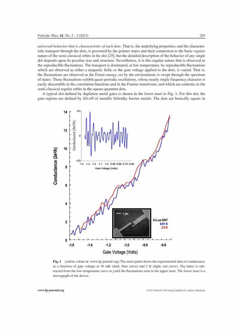
A typical dot defined by depletion metal gates is shown in the lower inset to Fig. 1. For this dot, thegate regions are defined by lift-off of metallic Schottky barrier metals. The dots are basically square in

Fig. 1 (online colour at: www.fp-journal.org) The main panel shows the experimental data of conductanceas a function of gate voltage at 10 mK (dark, blue curve) and 2 K (light, red curve). The latter is sub-tracted from the low temperature curve to yield the fluctuations seen in the upper inset. The lower inset is amicrograph of the device.

www.fp-journal.org © 2013 WILEY-VCH Verlag GmbH & Co. KGaA, Weinheim


nature, and sizes ranged from 1.5 μm to 0.4 μm (the electrical sizes are somewhat smaller due to edgedepletion around the gates). In nearly all cases studied, the carrier density was 3–5 ×1011 cm−2, andmobilities are typically 40–200 m2/V-s. The gate design allowed electrons to be trapped in the centralsquare cavity. Measurements were typically carried out at 10–300 mK base temperature in either a dilutionrefrigerator or a He3 cryostat, and source-drain excitation was kept well below the thermal voltage withlock-in techniques utilized. When the gate voltage is varied, the actual frequency depends upon both the dotsize and the lever arm from the gate voltage to the actual Fermi level motion within the dot. The oscillationsoften are observed over the entire range of gate voltage and persist to conductance values of 15 e2/h,which represents a very open dot. Here, we will focus upon a smaller dot, whose gate defined dimensionvaried from 0.2–0.3 micron, depending upon the value of the applied gate voltage. In the main panel ofFig. 1, we plot the conductance through the quantum dot as the gate voltage is varied. It may be seenthat the fluctuations ride on a uniformly increasing (for increasing gate voltage) conductance background.Rather than try to smooth the curve, the temperature is raised above 2 K, a point at which the fluctuationsare largely damped out, and the background appears as shown in the figure. This background curve isthen subtracted from the low temperature curve to isolate the fluctuations themselves, which are plottedas the upper inset in Fig. 1. These oscillations are very nearly periodic with a dominant period of about15 V−1 [26], although there are a few much weaker frequencies in the Fourier spectrum. The experimentalresults and quantum simulations yield the same dominant frequency in the dots [26]. Moreover, carefulstudies of the classical trajectories in such a dot have connected these scars to classical states on a KAMisland, and matched the corresponding frequencies. Certainly the change in the size of this island andthe change in dot size with gate voltage can be connected via careful determination of the self-consistentpotential, and this leads to a strong connection between the observed oscillations and the KAM islandstates [19, 22].

An extensive set of the conduction resonances/fluctuations has been examined for the projection ontothe single eigen-states (in each case), and the nature of the resonance has been shown to exhibit a Fanoline shape [27]. Here, it is found that the broadening of each resonance is essentially independent of thelead opening of the QPCs, so that the coupling of these states to the external world is through a processof phase space tunneling [19, 28]. That is, the current is assumed to enter the dot via one of the decoheredstates, tunnel to/from the pointer state, and then leave the dot via a second decohered state.Now, the pointerstates and the chaotic decohered states have different statistics. In particular, the classical regular states,and their quantum pointer state counterparts, have classical Poissonian statistics, while the chaotic statesare characterized by one of the Gaussian ensembles (the choice depends upon whether or not time reversalsymmetry is broken by a magnetic field). In fact, this difference in statistics has been measured in a quantumsimulation of the quantum dot [29]. This further serves as a clear connection between the classical and thequantum behavior that arises in these open quantum dots.

We have previously discussed the phase breaking time measurements that we have carried out on thesedots [24], so there here we will summarize the results. Generally, these are characterized by two distinctbehaviors. At low temperatures, the phase breaking time is independent of temperature, a result generallyin keeping with our understanding of the electron–electron interaction in mesoscopic systems [30]. At hightemperatures, however, the phase breaking time decreases as a power of the temperature, with the exponentbeing related to the dimensionality of the system. If the dot is coupled to a large two-dimensional system,this power law is T−1 [31]. However, if the dot is coupled to one dimensional wires at each QPC, thepower law appears to behave as T−2/3 [32]. These results are also consistent with the understanding of theelectron–electron interaction in mesoscopic systems [33]. Thus, this high temperature decay seems to indi-cate that the phase breaking process for the conductance oscillations, which arise from the pointer states, ischaracterized by the dimensionality of the environment to which the quantum dot is directly attached. Thatis, the dominant interaction for the phase breaking process arises from many-body interactions betweenelectrons on the pointer state and electrons in the environment. This is a slow process and phase breakingtimes of the order of a nanosecond can be observed for these open dots. We will return to this point below.


Fortschr. Phys. 61, No. 2 – 3 (2013) 295

3 The non-Hermitian Hamiltonian

Decoherence is thought to be an important part of the measurement process, especially in selecting the clas-sical results; that is, in passing from the quantum states to the measured classical states of a system [34].However, the description (and interpretation) of the decoherence process has varied widely, but key is theinteraction of the system upon the environment, as well as the interaction of the environment upon thesystem. Zurek has proposed that the interaction of the system on the environment leads to a preferred,discrete set of quantum states, known as pointer states, which remain robust, as their superposition withother states, and among themselves, is reduced by the decoherence process [35]. This decoherence-inducedselection of the preferred pointer states was termed einselection [34]. While this describes the physics ofeinselection, the mathematics can be shown by the use of projection operators. We give a brief overviewhere. We consider a system S, interacting with its environment E, so that the combined system plus en-vironment (S + E) is either closed, or influenced by external driving fields that are assumed known andunaffected by the feedback from this combined S+E. The Hilbert spaces of both the environment and thesystem are assumed to be finite dimensional, although this is not critical. These two spaces form a tensor-product Hilbert space of the system plus environment. The operators in which we are interested arecalledsuperoperators, and exist in an expanded space often called the Liouville space. When we open the dots,there will be an interaction between the dot and the environment, so that we can write the total Hamiltonianas

H = HS +HE +Hint, (1)

where the three terms represent the system, the environment, and the interaction between these two.There are two crucial steps in defining a reduced density matrix for just the pointer states. The first is to

project out these states via a projection superoperator. The second is to then trace over the environmentalstates yielding just the reduced set of pointer states. This procedure has been known for a considerable time[36–38]. There are many ways to define, or create, the necessary projection operator, which, as mentionedabove, is a commutator-generating superoperator. We want to choose the particular projection operatorsuch that

PHP = Hp, (2)

where the “caret” indicates a superoperator. Now, these projection operators are idempotent (P2 = P),and consequently have eigenvalues of 0 or 1, and it is a central tenet of quantum mechanics that we canbuild the system through knowledge of the eigen-functions and their eigen-values. For this subsystem, allthe eigenvectors are stationary states in the Heisenberg representation [39]. We have used this in an earlierstudy of open quantum systems [40]. With this approach, we recognize that the pointer states really are aset of isolated states within the dot, and are not directly coupled. Indeed, this approach has been used tocreate so-called decoherence-free subspaces in quantum information processing [41–43].

We begin by writing the Liouville equation in terms of the composite density matrix ρ, which is definedon a tensor product Hilbert space of the system density matrix and the environment density matrix, as

ρ = ρs ⊗ ρe, (3)

for which the Liouville equation can be written as

i �∂ρ

∂t= Hρ. (4)

In particular, the Hamiltonian is a commutator-generating superoperator. Equation (4) is easier to under-stand when we see that the Hamiltonian is now a 4th rank tensor, which generates the commutator relation



normally seen in this equation via

(Hρ)kn =∑

rs

Hkn,rsρrs

=∑

rs

(Hkrρrn − ρksHsn). (5)

If the dimension of ρs is ds and the dimension of ρe is de, then the dimension of the superoperator isd 2

s d 2e [40]. To simplify the approach, we Laplace transform (4), and then trace over the environment

variables to give [44]

(i�s − HS

)ρs = Tr (Hintρ) + ρs(0), (6)

As discussed above, we now use a projection operator which yields the pointer states as eigenfunctions.This operator has the basic properties

ρps = Pρs, P2 = P , Q = 1 − P . (7)

To proceed, we need only to use an identity that is obtained by projecting the Liouville equation with bothP and Q , solving for Qρs to formally decouple these two equations and recombining the terms [40, 45].This identity is

1

i �s − H=

(P + QRQH P

) 1

i �s− C − PH P

(P + PHQR

)+ PHQRQHP (8)

where

R =1

i �s − QHQ,

(9)

C = PHQRQHP .

The last term is a “collision” type term which connects the environment to the device via the off-diagonalelements of the superoperator. If we now define some further reduced parameters as

Σρps = Tre

(Cρps

),

(10)

H′intρps = Tre

(PH intPρs

)

we can then write the reduced equation as

i �(sρps − ρps(0)

)= Hpsρps + Σρps + H

′intρps + i �Tre

(PHQRQρs(0)

)(11)

In general, we are seeking the steady-state, long-time limit, and would ignore the initial conditions. How-ever, the last term in (11) has been suggested as contributing to the random force [46] that appears ine.g. the Langevin equation as well as to screening [47], so that it may not be proper to totally ignore it.However, the final long-time limit equation becomes, after inverting the Laplace transform,

i �∂ρps

∂t=

(Hps + H

′int

)ρps + Σρps (12)


Fortschr. Phys. 61, No. 2 – 3 (2013) 297

The second term on the right hand side is not a scattering, or decoherence term, as that would appearin the last term on the right. Instead, it represents a weak interaction between the pointer states and theenvironment via the decohered states. That is, it represents primarily the environment interaction on thenon-pointer states, which can then weakly couple to the pointer states. This term must represent the phasespace tunneling by which the pointer states appear in experiment [19]. It is true, however, that this canbring decoherence into the world of the pointer states via electron–electron interactions in the environmen-tal states, a point we have reviewed previously [24]. Normally, the pointer states do not interact with theenvironment, so that the last term would vanish, but the interaction of the pointer states, through the deco-hered states, to the environment produces the phase breaking discussed in the previous section. This meansthat the last term does not vanish, but represents this phase breaking process through an imaginary term inthis self-description. Since this scattering term is part of the Hamiltonian of the pointer states (the reducedset of states), it is a diagonal term, but has an imaginary part, which makes the Hamiltonian non-Hermitian.

It is important to remark here that this form of Hamiltonian is not what one normally refers to as non-Hermitian. Here, the imaginary term which breaks up the Hermitian properties lies on the diagonal ofthe matrix. In essence, this will also make the resulting reduced density matrix non-norm conserving asit breaks up the unity of the trace. But, this is because the germane interactions are from states withinthe dot and states of the environment, which can include renormalized decohered states of the dot. Thisenvironment sensitive dephasing interaction is seen in experiment [24], as discussed above. The steady-state situation has to then account for lost amplitude in the dot being replaced by electrons injected fromthe environment itself. These source terms must be incorporated within the first term on the right-hand sideof (12) as in any other transport problem.

Now, there are further problems with (12). While it appears to be quite simple conceptually, this isnot really the case. First, within the partial trace in both terms of (10), there is an explicit dependence onthe choice of the projection operator P or, equivalently, on the environment density matrix that inducesthe projection operator, so one must make a choice of the latter to actually be able to use (12). At theend of the day, the equation of motion for ρS(t) should not depend on it. And yet it does through itsaffects on the projection operator. The rationale for believing that the equation of motion for ρS(t) shouldnot depend on the details of the environment goes back to our statement above that the eigen-states ofρS(t) are our pointer states, and these are properties of the specific dot, and exist in the dot for a varietyof different environments. We have previously shown [40] that quite generally, the eigen-space of theprojection operator, corresponding to those states with eigenvalue 1, must be isomorphic to the states ofρS(t), which are our pointer states.

4 Quantum simulations

Since the pointer states conpose a reduced system, one must identify them before a projection operator canbe put together (which is mostly after we have the desired information). In general, this means a simulationof the quantum transport through the open quantum dot(s). Our method of choice for carrying out thequantum transport studies is one originally developed by Usuki and coworkers [48, 49]. It is a techniqueclosely related to the cascading scattering matrix approach, as well as the Green’s function approach whichmay be the most popular method for carrying out these kinds ofcalculations. The Usuki technique howeverhas a major advantage over the latter, as we will describe.

The starting point for our approach is a general Hamiltonian which is discretized upon a rectilineargrid [50]. While it is easy to incorporate the magnetic field, this approach has been extended to treatdissipation in nanowire transistors [51] and to incorporate spin and the Rashba and Dresselhaus spin-orbitterms [52]. On the grid, a tridiagonal matrix represents the Hamiltonian for the individual isolated slices I ,where a slice is the column of the grid normal to the direction of current flow. Expanding the Schrodingerequation discretization, one obtains an iterative equation for one slice in terms of the previous ones, whichis a form of the Lippmann-Schwinger equation on the grid. Coupling this with the trivial equation that the



slice wave function vectors are equal to each other, one can derive a transfer-matrix equation that relatesadjacent slices, as

[⇀

ψi⇀

ψi+1

]=

⎡

⎢⎣0 I

−I(

H0i − Et

)⎤

⎥⎦

[⇀

ψi−1⇀

ψi

]= Ti

[⇀

ψi−1⇀

ψi

](13)

where t = �2/(2m∗a2) is the hopping matrix element from one site to the next. Here, this acts as a weak

perturbation coupling one slice to the next, and is of course modified in a magnetic field via the Peierls’phase. One begins the calculation by turning to Bloch’s theorem, and solving the eigenvalue problem forthe transfer-matrix on the first slice (the T matrix carries throughout by coupling one slice to the next)

T1

[⇀

ψ1⇀

ψ0

]=

[T11 T12

T12 T22

] [⇀

ψ1⇀

ψ0

]= λ

[⇀

ψ1⇀

ψ0

]. (14)

Once one has passed the initialization of the transfer matrices with the initial conditions on the wavefunction, which are defined through the matrices C0

1 =I and C02 = 0. These are defined for the zero slice.

Then the general iteration becomes[

Cl+11 Cl+1

2

0 I

]= Tl

[Cl

1 Cl2

0 I

]Pl, (15)

where

Pl =

[I 0

Pl1 Pl1

], (16a)

with

Pl1 = −Pl2Tl21Cl1, (16b)

and

Pl2 =(

Tl21Cl2 + Tl22

) −1

. (16c)

The numerical stability of the Usuki et al. method in large part stems from the fact that the iteration impliedby (15) involves products of matrices with inverted matrices. Taking such products tends to cancel out mostof the troublesome exponential factors.

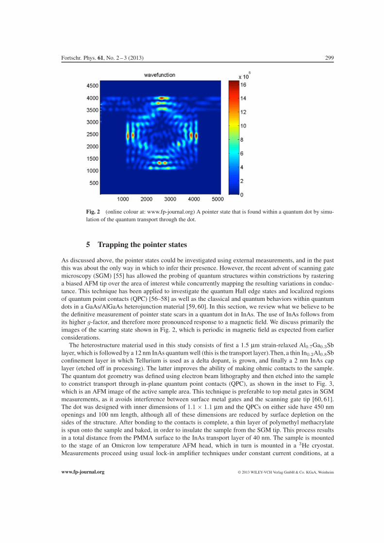
In Fig. 2, we display a scarred wave function which is found in a nominally 0.3 μm square dot with40 nm QPCs, located at the top edge of the dot (it is possible to note the modes which are passing throughthese QPCs at the top of the figure), which pass three modes. This wave function appears periodically inmagnetic field, almost always with essentially the same shape, and thus is one of the pointer states. Thisstate is very long lived and clearly identified with the dot itself. Moreover, it is found that this scarred statescales with the dot size [53,54]. The wave function shown in Fig. 2 is clearly scarred by a periodic classicalorbit. However, since the structure is ostensibly regular, the fact that there appears to be a correspondenceto the classical picture should not be a surprise (as pointed out above) since the wave functions should beconcentrated along the projections of the invariant tori of the regular trajectories in classical phase space.However, it is worth pointing out that this image differs radically from what occurs in a closed dot, in whichthe amplitude for an eigenstate is distributed much more uniformly and one can not make an associationwith a single orbit. It is also worth noting that this wave function does not have significant amplitude at theQPCs, but is basically isolated from them.


Fortschr. Phys. 61, No. 2 – 3 (2013) 299

Fig. 2 (online colour at: www.fp-journal.org) A pointer state that is found within a quantum dot by simu-lation of the quantum transport through the dot.

5 Trapping the pointer states

As discussed above, the pointer states could be investigated using external measurements, and in the pastthis was about the only way in which to infer their presence. However, the recent advent of scanning gatemicroscopy (SGM) [55] has allowed the probing of quantum structures within constrictions by rasteringa biased AFM tip over the area of interest while concurrently mapping the resulting variations in conduc-tance. This technique has been applied to investigate the quantum Hall edge states and localized regionsof quantum point contacts (QPC) [56–58] as well as the classical and quantum behaviors within quantumdots in a GaAs/AlGaAs heterojunction material [59, 60]. In this section, we review what we believe to bethe definitive measurement of pointer state scars in a quantum dot in InAs. The use of InAs follows fromits higher g-factor, and therefore more pronounced response to a magnetic field. We discuss primarily theimages of the scarring state shown in Fig. 2, which is periodic in magnetic field as expected from earlierconsiderations.

The heterostructure material used in this study consists of first a 1.5 μm strain-relaxed Al0.7Ga0.3Sblayer, which is followed by a 12 nm InAs quantum well (this is the transport layer).Then, a thin In0.2Al0.8Sbconfinement layer in which Tellurium is used as a delta dopant, is grown, and finally a 2 nm InAs caplayer (etched off in processing). The latter improves the ability of making ohmic contacts to the sample.The quantum dot geometry was defined using electron beam lithography and then etched into the sampleto constrict transport through in-plane quantum point contacts (QPC), as shown in the inset to Fig. 3,which is an AFM image of the active sample area. This technique is preferable to top metal gates in SGMmeasurements, as it avoids interference between surface metal gates and the scanning gate tip [60, 61].The dot was designed with inner dimensions of 1.1 × 1.1 μm and the QPCs on either side have 450 nmopenings and 100 nm length, although all of these dimensions are reduced by surface depletion on thesides of the structure. After bonding to the contacts is complete, a thin layer of polymethyl methacrylateis spun onto the sample and baked, in order to insulate the sample from the SGM tip. This process resultsin a total distance from the PMMA surface to the InAs transport layer of 40 nm. The sample is mountedto the stage of an Omicron low temperature AFM head, which in turn is mounted in a 3He cryostat.Measurements proceed using usual lock-in amplifier techniques under constant current conditions, at a



0.0

0.2

0.4

0.6

0.8

1.0

0 10 20 30 40 50

Fou

rier

Cou

nt [a

.u.]

Magnetic Frequency [T -1]

500 nm

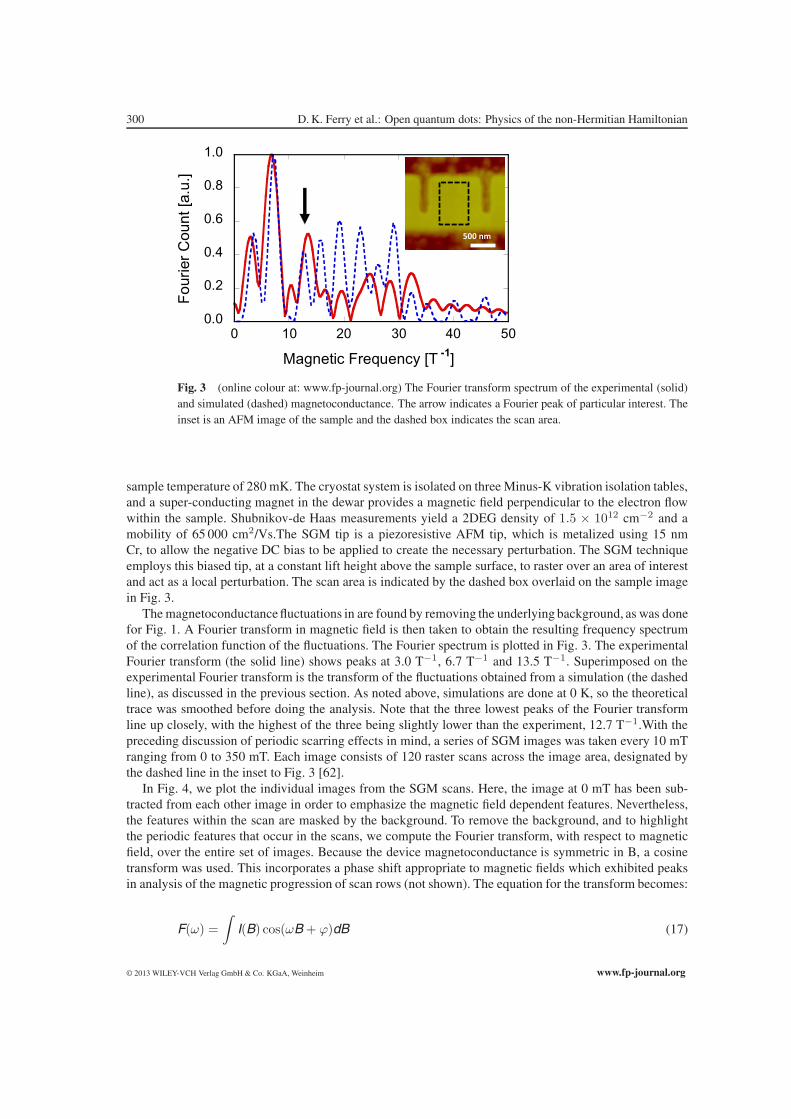
Fig. 3 (online colour at: www.fp-journal.org) The Fourier transform spectrum of the experimental (solid)and simulated (dashed) magnetoconductance. The arrow indicates a Fourier peak of particular interest. Theinset is an AFM image of the sample and the dashed box indicates the scan area.

sample temperature of 280 mK. The cryostat system is isolated on three Minus-K vibration isolation tables,and a super-conducting magnet in the dewar provides a magnetic field perpendicular to the electron flowwithin the sample. Shubnikov-de Haas measurements yield a 2DEG density of 1.5 × 1012 cm−2 and amobility of 65 000 cm2/Vs.The SGM tip is a piezoresistive AFM tip, which is metalized using 15 nmCr, to allow the negative DC bias to be applied to create the necessary perturbation. The SGM techniqueemploys this biased tip, at a constant lift height above the sample surface, to raster over an area of interestand act as a local perturbation. The scan area is indicated by the dashed box overlaid on the sample imagein Fig. 3.

The magnetoconductance fluctuations in are found by removing the underlying background, as was donefor Fig. 1. A Fourier transform in magnetic field is then taken to obtain the resulting frequency spectrumof the correlation function of the fluctuations. The Fourier spectrum is plotted in Fig. 3. The experimentalFourier transform (the solid line) shows peaks at 3.0 T−1, 6.7 T−1 and 13.5 T−1. Superimposed on theexperimental Fourier transform is the transform of the fluctuations obtained from a simulation (the dashedline), as discussed in the previous section. As noted above, simulations are done at 0 K, so the theoreticaltrace was smoothed before doing the analysis. Note that the three lowest peaks of the Fourier transformline up closely, with the highest of the three being slightly lower than the experiment, 12.7 T−1.With thepreceding discussion of periodic scarring effects in mind, a series of SGM images was taken every 10 mTranging from 0 to 350 mT. Each image consists of 120 raster scans across the image area, designated bythe dashed line in the inset to Fig. 3 [62].

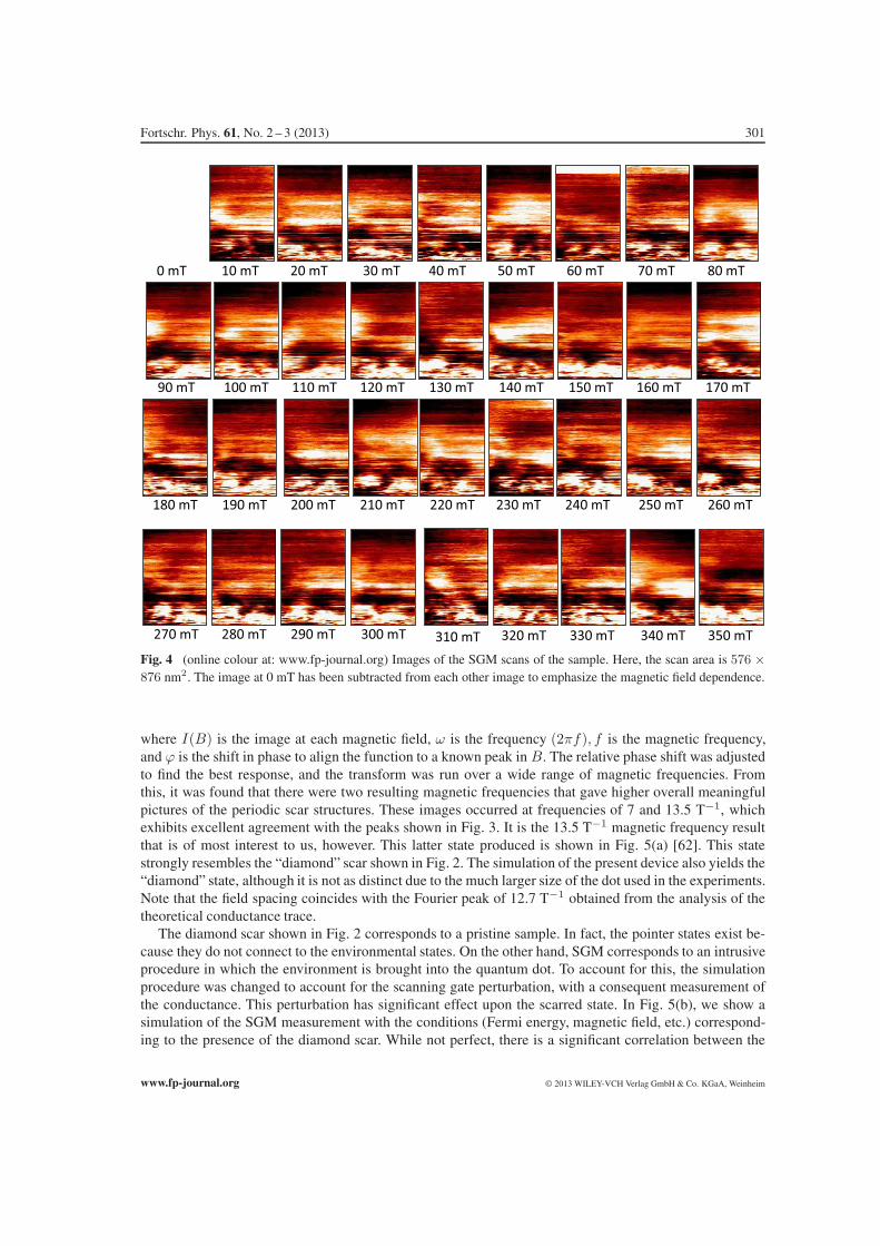
In Fig. 4, we plot the individual images from the SGM scans. Here, the image at 0 mT has been sub-tracted from each other image in order to emphasize the magnetic field dependent features. Nevertheless,the features within the scan are masked by the background. To remove the background, and to highlightthe periodic features that occur in the scans, we compute the Fourier transform, with respect to magneticfield, over the entire set of images. Because the device magnetoconductance is symmetric in B, a cosinetransform was used. This incorporates a phase shift appropriate to magnetic fields which exhibited peaksin analysis of the magnetic progression of scan rows (not shown). The equation for the transform becomes:

F(ω) =∫

I(B) cos(ωB + ϕ)dB (17)


Fortschr. Phys. 61, No. 2 – 3 (2013) 301

0 mT 10 mT 20 mT 30 mT 50 mT40 mT 60 mT 70 mT 80 mT

90 mT 100 mT 110 mT 130 mT120 mT 150 mT140 mT 160 mT 170 mT

180 mT 190 mT 200 mT 210 mT 220 mT 240 mT230 mT 260 mT250 mT

270 mT 280 mT 290 mT 300 mT 310 mT 320 mT 330 mT 350 mT340 mT

Fig. 4 (online colour at: www.fp-journal.org) Images of the SGM scans of the sample. Here, the scan area is 576 ×876 nm2. The image at 0 mT has been subtracted from each other image to emphasize the magnetic field dependence.

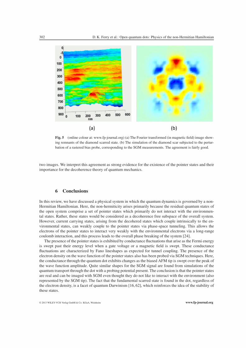
where I(B) is the image at each magnetic field, ω is the frequency (2πf), f is the magnetic frequency,and ϕ is the shift in phase to align the function to a known peak in B. The relative phase shift was adjustedto find the best response, and the transform was run over a wide range of magnetic frequencies. Fromthis, it was found that there were two resulting magnetic frequencies that gave higher overall meaningfulpictures of the periodic scar structures. These images occurred at frequencies of 7 and 13.5 T−1, whichexhibits excellent agreement with the peaks shown in Fig. 3. It is the 13.5 T−1 magnetic frequency resultthat is of most interest to us, however. This latter state produced is shown in Fig. 5(a) [62]. This statestrongly resembles the “diamond” scar shown in Fig. 2. The simulation of the present device also yields the“diamond” state, although it is not as distinct due to the much larger size of the dot used in the experiments.Note that the field spacing coincides with the Fourier peak of 12.7 T−1 obtained from the analysis of thetheoretical conductance trace.

The diamond scar shown in Fig. 2 corresponds to a pristine sample. In fact, the pointer states exist be-cause they do not connect to the environmental states. On the other hand, SGM corresponds to an intrusiveprocedure in which the environment is brought into the quantum dot. To account for this, the simulationprocedure was changed to account for the scanning gate perturbation, with a consequent measurement ofthe conductance. This perturbation has significant effect upon the scarred state. In Fig. 5(b), we show asimulation of the SGM measurement with the conditions (Fermi energy, magnetic field, etc.) correspond-ing to the presence of the diamond scar. While not perfect, there is a significant correlation between the



Fig. 5 (online colour at: www.fp-journal.org) (a) The Fourier transformed (in magnetic field) image show-ing remnants of the diamond scarred state. (b) The simulation of the diamond scar subjected to the pertur-bation of a rastered bias probe, corresponding to the SGM measurements. The agreement is fairly good.

two images. We interpret this agreement as strong evidence for the existence of the pointer states and theirimportance for the decoherence theory of quantum mechanics.

6 Conclusions

In this review, we have discussed a physical system in which the quantum dynamics is governed by a non-Hermitian Hamiltonian. Here, the non-hermiticity arises primarily because the residual quantum states ofthe open system comprise a set of pointer states which primarily do not interact with the environmen-tal states. Rather, these states would be considered as a decoherence free subspace of the overall system.However, current carrying states, arising from the decohered states which couple intrinsically to the en-vironmental states, can weakly couple to the pointer states via phase-space tunneling. This allows theelectrons of the pointer states to interact very weakly with the environmental electrons via a long-rangecoulomb interaction, and this process leads to the overall phase breaking of the system [24].

The presence of the pointer states is exhibited by conductance fluctuations that arise as the Fermi energyis swept past their energy level when a gate voltage or a magnetic field is swept. These conductancefluctuations are characterized by Fano lineshapes as expected for tunnel coupling. The presence of theelectron density on the wave function of the pointer states also has been probed via SGM techniques. Here,the conductance through the quantum dot exhibits changes as the biased AFM tip is swept over the peak ofthe wave function amplitude. Quite similar shapes for the SGM signal are found from simulations of thequantum transport through the dot with a probing potential present. The conclusion is that the pointer statesare real and can be imaged with SGM even thought they do not like to interact with the environment (alsorepresented by the SGM tip). The fact that the fundamental scarred state is found in the dot, regardless ofthe electron density, is a facet of quantum Darwinism [16, 62], which reinforces the idea of the stability ofthese states.


Fortschr. Phys. 61, No. 2 – 3 (2013) 303

References

[1] J. A. Wheeler and W. H. Zurek, (eds.) Quantum Theory and Measurement (Princeton University Press, Prince-ton, NJ, 1983).

[2] J. P. Bird, R. Akis, D. K. Ferry, and M. Stopa, in: Advances in Imaging and Electron Physics, Vol. 107, editedby P. Hawkes (Academic Press, San Diego, 1999, pp. 1–71.

[3] C. W. J. Beenakker and H. van Houten, Solid State Phys. 44, 1 (1991).[4] C. M. Marcus et al., Phys. Rev. Lett. 69, 506 (1992).[5] A. M. Chang et al., Phys. Rev. Lett. 73, 2111 (1994).[6] R. P. Taylor et al., Phys. Rev. B 51, 9801 (1995).[7] J. P. Bird et al., Phys. Rev. B 51, 18037 (1995).[8] M. Persson et al., Phys. Rev. B 52, 8921 (1995).[9] M. W. Keller et al., Phys. Rev B 53, R1693 (1996).

[10] R. A. Jalabert, H. U. Baranger, and A. D. Stone, Phys. Rev. Lett. 65, 2442 (1990).[11] H. U. Baranger, R. A. Jalabert, and A. D. Stone, Phys. Rev. Lett. 70, 3876 (1993).[12] R. Akis, D. K. Ferry, and J. P. Bird, Phys. Rev. B 54, 17705 (1996).[13] R. Akis, D. K. Ferry, and J. P. Bird, Phys. Rev. Lett. 79, 123 (1997).[14] W. H. Zurek, Rev. Mod. Phys. 75, 715 (2003).[15] H. Ollivier, D. Poulin, and W. H. Zurek, Phys. Rev. Lett. 93, 220401 (2004).[16] R. Blume-Kohout and W. H. Zurek, Phys. Rev. Lett. 101, 240405 (2008).[17] C. Darwin, The Origin of Species (Jon Murray, London, 1859).[18] R. Ketzmerick, Phys. Rev. B 54, 10841 (1996).[19] A. P. S. De Moura et al., Phys. Rev. Lett. 88, 236804 (2002).[20] D. K. Ferry, R. Akis, and J. P. Bird, Phys. Rev. Lett. 93, 026803 (2004).[21] D. K. Ferry et al., Semicond. Sci. Technol. 26, 043001 (2011).[22] R. Brunner et al., J. Phys., Condens. Matter. (in press).[23] R. Brunner et al., Phys. Rev. Lett. 101, 024102 (2008).[24] D. K. Ferry, R. Akis, and J. P. Bird, J. Phys., Condens. Matter. 17, 1017 (2005).[25] J. P. Bird et al., Rep. Progr. Phys. 66, 583 (2003).[26] J. P. Bird et al., Phys. Rev. Lett. 82, 4691 (1999).[27] R. Akis, J. P. Bird, and D. K. Ferry, Microelectron. Eng. 63, 241 (2002).[28] R. Akis et al., J. Comput. Electron. 2, 281 (2003).[29] R. Akis and D. K. Ferry, Physica E 34, 460 (2006).[30] D. K. Ferry, Semiconductor Transport (Taylor & Francis, London, 2000) pp. 355–359.[31] J. P. Bird et al., Phys. Status Solidi (b) 204, 314 (1997).[32] D. P. Pivin Jr. et al., Phys. Rev. Lett. 82, 4687 (1999).[33] B. L. Altshuler, A. G. Aronov, and D. E. Khmelnitsky, J. Phys. C 15, 7367 (1982).[34] W. H. Zurek, Phys. Rev. D 26, 1862 (1982).[35] W. H. Zurek, Phys. Rev. D 24, 1516 (1981).[36] S. Nakajima, Prog. Theor. Phys. 20, 948 (1958).[37] R. Zwanzig, J. Chem. Phys. 33, 1338 (1960).[38] H. Mori, Prog. Theor. Phys. 33, 423 (1965).[39] P. A. M. Dirac, The Principles of Quantum Mechanics, 4th edition (Oxford University Press, London, 1958).[40] I. Knezevic and D. K. Ferry, Phys. Rev. E 66, 016131 (2002).[41] L. M. Duan and G. C. Guo, Phys. Rev. A 57, 737 (1998).[42] P. Zanardi and M. Rasetti, Phys. Rev. Lett. 79, 3306 (1997).[43] D. A. Lidar, I. L. Chuang, and K. B. Whaley, Phys. Rev. Lett. 81, 2594 (1998).[44] D. K. Ferry, Semiconductors, Chapter 15 (Macmillan, New York, 1991).[45] J. R. Barker, Solid-State Electron. 21, 197 (1978).[46] N. Pottier, Physica A 117, 243 (1983).[47] J. R. Barker, in: Physics of Nonlinear Transport in Semiconductors, edited by D. K. Ferry, J. R. Barker, and

C. Jacoboni (Plenum Press, New York, 1979).[48] T. Usuki et al., Phys. Rev. B 50, 7615 (1994).



[49] T. Usuki et al., Phys. Rev. B 52, 8244 (1995).[50] R. Akis et al., in: Electron Transport in Quantum Dots, edited by J. P. Bird (Kluwer Academic Publishers,

Boston, 2003) pp. 209–276.[51] M. J. Gilbert, R. Akis, and D. K. Ferry, J. Appl. Phys. 98, 094303 (2005).[52] A. W. Cummings, R. Akis, and D. K. Ferry, J. Phys., Condens. Matter. 23, 465301 (2011).[53] J. P. Bird et al., Chaos, Solitons, Fractals 8, 1299 (1997).[54] D. K. Ferry et al., Jpn. J. Appl. Phys. 36, 3944 (1997).[55] M. A. Topinka et al., Science 289, 2323 (2000).[56] R. Crook et al., J. Phys. Cond. Matt. 12, L167 (2000).[57] N. Aoki et al., Phys. Rev. B 72, 155327 (2005).[58] C. R. da Cunha et al., Appl. Phys. Lett. 89, 242109 (2006).[59] R. Crook et al., Phys. Rev. Lett. 91 246803 (2003).[60] A. M. Burke et al., J. Vac. Sci. Technol. B 26, 1488 (2008).[61] A. M. Burke et al., J. Phys., Condens. Matter. 21, 202201 (2009).[62] A. M. Burke et al., Phys. Rev. Lett. 104, 176801 (2010).


open quantum dots: physics of the non-hermitian...

Documents