Least Squares Multi-Window Evolutionary Spectral Estimation

MAHMUT YALCIN, AYDIN AKAN and MAHMUT OZTURKIstanbul University, Department of Electrical and Electronics Engineering

Avcilar, Istanbul, 34580, TURKEY

Abstract: -We present a multi–window method for obtaining the time-frequency spectrum of of non-stationary signals such as speech and music. This method is based on optimal combination of evolu-tionary spectra that are calculated by using multi–window Gabor expansion. The optimal weights areobtained by using a least square estimation method. An error criterion that is the squared distance be-tween a reference time–frequency distribution and the combination of evolutionary spectra is minimizedto determine the weights. Examples are given to illustrate the effectiveness of the proposed method.

Key-Words: -Time-frequency analysis, Evolutionary spectrum, Multi-window time-frequency analysis.

1 IntroductionTime–Frequency (TF) signal analysis is a help-ful tool for analyzing the time–varying frequencycontent of non–stationary signals such as speech,music, biological signals etc. [1]. For a time-dependent spectral analysis of non–stationarystochastic process, the Wigner-Ville Spectrum(WVS) [2] is given by :

S (t, ω) = E {W (t, ω)}= E

{∫ ∞

−∞[x(t− τ

2) x∗(t +

τ

2)] e−jωτdτ

}

whereW (t, ω) denotes the Wigner Distribution(WD) and the above is the statistical average ofthe WDs of the realizations of the process. Whenwe have several observations of the non–stationaryprocessx(t), we can use an ensemble average ofthe individual WDs of these observations to esti-mate the WVS. However, this is not the case ingeneral; we are only given a single realization ofthe process. In that case, Time–Frequency Distri-butions (TFDs) with a smoothing kernel functionis used to estimate the WVS [1]. A good amountof research has been done to design kernels with

1 This work was supported by the Research Fund of TheUniversity of Istanbul, Project numbers: BYP-6/05062002and B-1080/27062001.

desired properties yielding unbiased and low vari-ance WVS estimates [4, 2]. A new estimate ofthe WVS is proposed as an optimal average ofmultiple-window spectrograms of the process in[5, 6] in the least squares sense. In this work weextend this WVS estimate to the weighted averagecombination of multi-window evolutionary spec-tra obtained by a Discrete Evolutionary Transform(DET) [9]. The combination weights are deter-mined by minimizing a sum-squared difference(norm squared distance) between the average evo-lutionary spectrum and a higher order TF repre-sentation.

There is a growing interest on higher ordertime-frequency methods. One example is the classof Time-Varying Higher Order Spectra (TV-HOS)based on Polynomial Wigner-Ville Distributions(PWVD) [11, 12, 14]. Higher order TF meth-ods are useful in the analysis of non–linear, non–Gaussian signals. Several methods have been pre-sented to estimate a time–varying spectrum us-ing higher order statistics. In [12], it has beenshown that PWVD can achieve the delta functionconcentration for polynomial FM signals (that issignals with the instantaneous phase modelled bya polynomial of possibly order higher than two).TV-HOS have been recently developed in a searchfor a tool that could perform higher-order spec-

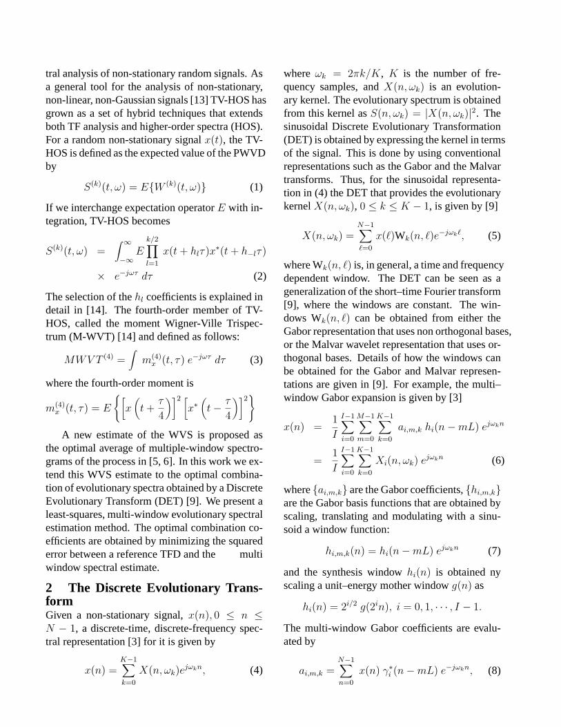
tral analysis of non-stationary random signals. Asa general tool for the analysis of non-stationary,non-linear, non-Gaussian signals [13] TV-HOS hasgrown as a set of hybrid techniques that extendsboth TF analysis and higher-order spectra (HOS).For a random non-stationary signalx(t), the TV-HOS is defined as the expected value of the PWVDby

S(k)(t, ω) = E{W (k)(t, ω)} (1)

If we interchange expectation operatorE with in-tegration, TV-HOS becomes

S(k)(t, ω) =∫ ∞

−∞E

k/2∏

l=1

x(t + hlτ)x∗(t + h−lτ)

× e−jωτ dτ (2)

The selection of thehl coefficients is explained indetail in [14]. The fourth-order member of TV-HOS, called the moment Wigner-Ville Trispec-trum (M-WVT) [14] and defined as follows:

MWV T (4) =∫

m(4)x (t, τ) e−jωτ dτ (3)

where the fourth-order moment is

m(4)x (t, τ) = E

{[x

(t +

τ

4

)]2 [x∗

(t− τ

4

)]2}

A new estimate of the WVS is proposed asthe optimal average of multiple-window spectro-grams of the process in [5, 6]. In this work we ex-tend this WVS estimate to the optimal combina-tion of evolutionary spectra obtained by a DiscreteEvolutionary Transform (DET) [9]. We present aleast-squares, multi-window evolutionary spectralestimation method. The optimal combination co-efficients are obtained by minimizing the squarederror between a reference TFD and the multiwindow spectral estimate.

2 The Discrete Evolutionary Trans-formGiven a non-stationary signal,x(n), 0 ≤ n ≤N − 1, a discrete-time, discrete-frequency spec-tral representation [3] for it is given by

x(n) =K−1∑

k=0

X(n, ωk)ejωkn, (4)

whereωk = 2πk/K, K is the number of fre-quency samples, andX(n, ωk) is an evolution-ary kernel. The evolutionary spectrum is obtainedfrom this kernel asS(n, ωk) = |X(n, ωk)|2. Thesinusoidal Discrete Evolutionary Transformation(DET) is obtained by expressing the kernel in termsof the signal. This is done by using conventionalrepresentations such as the Gabor and the Malvartransforms. Thus, for the sinusoidal representa-tion in (4) the DET that provides the evolutionarykernelX(n, ωk), 0 ≤ k ≤ K − 1, is given by [9]

X(n, ωk) =N−1∑

`=0

x(`)Wk(n, `)e−jωk`, (5)

where Wk(n, `) is, in general, a time and frequencydependent window. The DET can be seen as ageneralization of the short–time Fourier transform[9], where the windows are constant. The win-dows Wk(n, `) can be obtained from either theGabor representation that uses non orthogonal bases,or the Malvar wavelet representation that uses or-thogonal bases. Details of how the windows canbe obtained for the Gabor and Malvar represen-tations are given in [9]. For example, the multi–window Gabor expansion is given by [3]

x(n) =1

I

I−1∑

i=0

M−1∑

m=0

K−1∑

k=0

ai,m,k hi(n−mL) ejωkn

=1

I

I−1∑

i=0

K−1∑

k=0

Xi(n, ωk) ejωkn (6)

where{ai,m,k} are the Gabor coefficients,{hi,m,k}are the Gabor basis functions that are obtained byscaling, translating and modulating with a sinu-soid a window function:

hi,m,k(n) = hi(n−mL) ejωkn (7)

and the synthesis windowhi(n) is obtained nyscaling a unit–energy mother windowg(n) as

hi(n) = 2i/2 g(2in), i = 0, 1, · · · , I − 1.

The multi-window Gabor coefficients are evalu-ated by

ai,m,k =N−1∑

n=0

x(n) γ∗i (n−mL) e−jωkn, (8)

where the analysis windowγi(n) is solved fromthe bi-orthogonality condition betweenhi(n) andγi(n) [3]. The evolutionary kernel is obtained bycomparing the spectral and the Gabor representa-tions of the signal (6):

Xi(n, ωk) =M−1∑

m=0

ai,m,k hi(n−mL) (9)

Replacing for the coefficients{ai,m,k}, one canalso write

Xi(n, ωk) =N−1∑

`=0

x(`) Wi(n, `) e−jωk`, (10)

where the time–varying window for scale2i is de-fined as

Wi(n, `) =M−1∑

m=0

γ∗i (`−mL) hi(n−mL).

Then the evolutionary spectrum ofx(n) calculatedby the window Wi(n, `) is

Si(n, ωk) =1

K|Xi(n, ωk)|2,

where the factor1/K is used for proper energynormalization. We should mention that normal-izing the Wi(n, `) to unit energy, the total energyof the signal is preserved thus justifying the useof Si(n, ωk) as a TF representation forx(n). Fur-thermore,Si(n, ωk) is always non–negative andapproximates the marginal conditions [1]; hence,in contrast to many TFDs, interpretable as TF en-ergy density function [3].

3 Least Squares Evolutionary Spec-trumGiven a realization of a discrete-time, nonstation-ary process corrupted by additive noisex(n) =s(n) + η(n) wheres(n) andη(n) denotes the sig-nal and noise processes respectively. We intendto obtain a high resolution evolutionary spectralestimate with good performance in low signal tonoise ratio (SNR) conditions. We calculate a we-ighted average combination of evolutionary spec-tra Si(n, ωk) that is closest to a reference TFD in

a least squares sense. Given the signalx(n), wecalculate evolutionary spectraSi(n, ωk) for i =0, 1, · · · , I − 1 as

Si(n, ωk) =1

K

∣∣∣∣∣N−1∑

`=0

x(`) Wi(n, `) e−jωk`

∣∣∣∣∣

2

.

(11)Gauss windows are used ashi(n), for their op-timal concentration in the TF plane [10]. Thenwe estimate the WVS of the processx(n) as aweighted average of the evolutionary spectra

P (n, ωk) =I−1∑

i=0

ci Si(n, ωk) (12)

where the weights{ci} are obtained by minimiz-ing the error function

εi =N−1∑

n=0

K−1∑

k=0

∣∣∣∣∣PR(n, ωk)−I−1∑

i=0

ciSi(n, ωk)

∣∣∣∣∣

2

(13)

andPR(n, ωk) is a reference TFD which is takenhere as higher order TF representation [11] of thesignal.

By using a matrix notation, the minimizationproblem in (13) can be rewritten as

minci||PR − S c||2 (14)

The solution of this least squares minimizationproblem is

co = (STS)−1STPR

where the superscript ‘o ’ stands for optimum.Then a WVS estimate is obtained as optimalweighted average using{co

i} as

PES(n, ωk) =I−1∑

i=0

coi Si(n, ωk) (15)

Finally, we mask or threshold our estimate to elim-inate any possible negative values as in [6], andresult in a non–negative time–varying spectrum,i.e.,

PES(n, ωk)+ =

{P (n, ωk), P (n, ωk) ≥ 0;0, P (n, ωk) < 0.

(16)

wherePES(n, ωk)+ denotes the positive-only part

of the evolutionary spectrum.

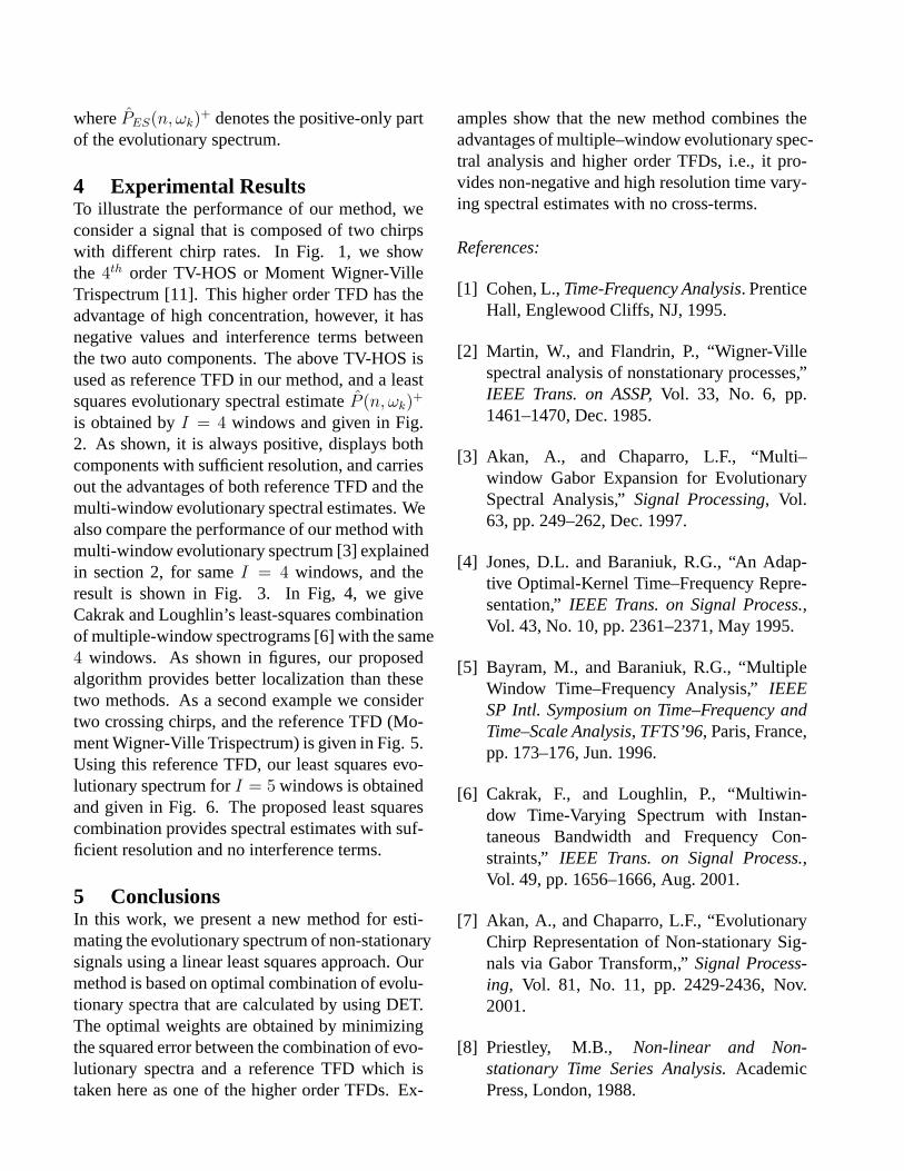
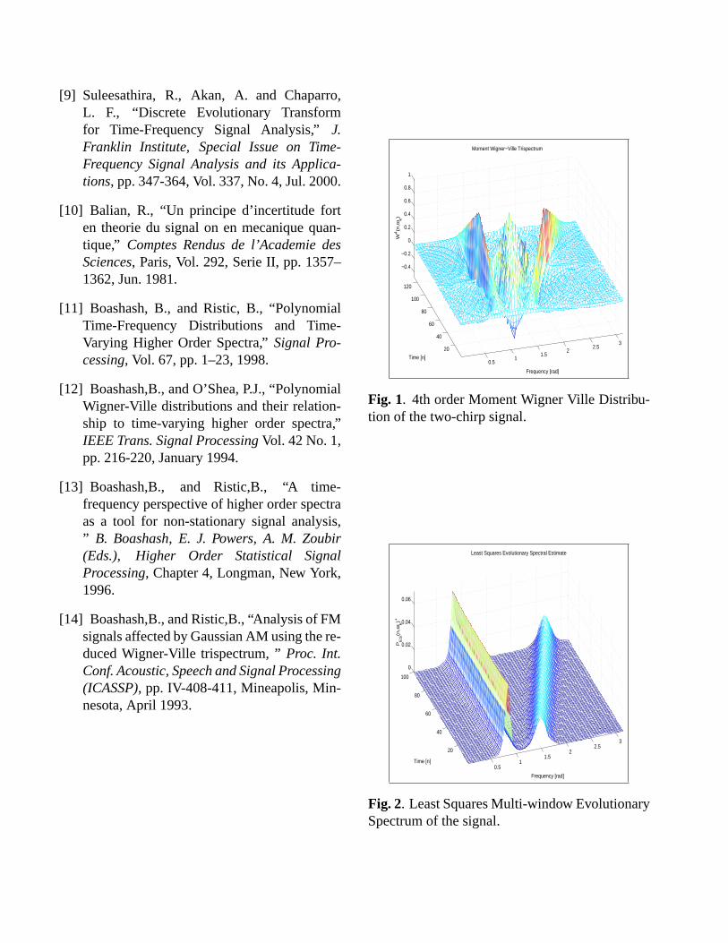
4 Experimental ResultsTo illustrate the performance of our method, weconsider a signal that is composed of two chirpswith different chirp rates. In Fig. 1, we showthe 4th order TV-HOS or Moment Wigner-VilleTrispectrum [11]. This higher order TFD has theadvantage of high concentration, however, it hasnegative values and interference terms betweenthe two auto components. The above TV-HOS isused as reference TFD in our method, and a leastsquares evolutionary spectral estimateP (n, ωk)

+

is obtained byI = 4 windows and given in Fig.2. As shown, it is always positive, displays bothcomponents with sufficient resolution, and carriesout the advantages of both reference TFD and themulti-window evolutionary spectral estimates. Wealso compare the performance of our method withmulti-window evolutionary spectrum [3] explainedin section 2, for sameI = 4 windows, and theresult is shown in Fig. 3. In Fig, 4, we giveCakrak and Loughlin’s least-squares combinationof multiple-window spectrograms [6] with the same4 windows. As shown in figures, our proposedalgorithm provides better localization than thesetwo methods. As a second example we considertwo crossing chirps, and the reference TFD (Mo-ment Wigner-Ville Trispectrum) is given in Fig. 5.Using this reference TFD, our least squares evo-lutionary spectrum forI = 5 windows is obtainedand given in Fig. 6. The proposed least squarescombination provides spectral estimates with suf-ficient resolution and no interference terms.

5 ConclusionsIn this work, we present a new method for esti-mating the evolutionary spectrum of non-stationarysignals using a linear least squares approach. Ourmethod is based on optimal combination of evolu-tionary spectra that are calculated by using DET.The optimal weights are obtained by minimizingthe squared error between the combination of evo-lutionary spectra and a reference TFD which istaken here as one of the higher order TFDs. Ex-

amples show that the new method combines theadvantages of multiple–window evolutionary spec-tral analysis and higher order TFDs, i.e., it pro-vides non-negative and high resolution time vary-ing spectral estimates with no cross-terms.

References:

[1] Cohen, L.,Time-Frequency Analysis. PrenticeHall, Englewood Cliffs, NJ, 1995.

[2] Martin, W., and Flandrin, P., “Wigner-Villespectral analysis of nonstationary processes,”IEEE Trans. on ASSP,Vol. 33, No. 6, pp.1461–1470, Dec. 1985.

[3] Akan, A., and Chaparro, L.F., “Multi–window Gabor Expansion for EvolutionarySpectral Analysis,”Signal Processing, Vol.63, pp. 249–262, Dec. 1997.

[4] Jones, D.L. and Baraniuk, R.G., “An Adap-tive Optimal-Kernel Time–Frequency Repre-sentation,”IEEE Trans. on Signal Process.,Vol. 43, No. 10, pp. 2361–2371, May 1995.

[5] Bayram, M., and Baraniuk, R.G., “MultipleWindow Time–Frequency Analysis,”IEEESP Intl. Symposium on Time–Frequency andTime–Scale Analysis, TFTS’96, Paris, France,pp. 173–176, Jun. 1996.

[6] Cakrak, F., and Loughlin, P., “Multiwin-dow Time-Varying Spectrum with Instan-taneous Bandwidth and Frequency Con-straints,” IEEE Trans. on Signal Process.,Vol. 49, pp. 1656–1666, Aug. 2001.

[7] Akan, A., and Chaparro, L.F., “EvolutionaryChirp Representation of Non-stationary Sig-nals via Gabor Transform,,”Signal Process-ing, Vol. 81, No. 11, pp. 2429-2436, Nov.2001.

[8] Priestley, M.B., Non-linear and Non-stationary Time Series Analysis.AcademicPress, London, 1988.

[9] Suleesathira, R., Akan, A. and Chaparro,L. F., “Discrete Evolutionary Transformfor Time-Frequency Signal Analysis,”J.Franklin Institute, Special Issue on Time-Frequency Signal Analysis and its Applica-tions, pp. 347-364, Vol. 337, No. 4, Jul. 2000.

[10] Balian, R., “Un principe d’incertitude forten theorie du signal on en mecanique quan-tique,” Comptes Rendus de l’Academie desSciences, Paris, Vol. 292, Serie II, pp. 1357–1362, Jun. 1981.

[11] Boashash, B., and Ristic, B., “PolynomialTime-Frequency Distributions and Time-Varying Higher Order Spectra,”Signal Pro-cessing, Vol. 67, pp. 1–23, 1998.

[12] Boashash,B., and O’Shea, P.J., “PolynomialWigner-Ville distributions and their relation-ship to time-varying higher order spectra,”IEEE Trans. Signal ProcessingVol. 42 No. 1,pp. 216-220, January 1994.

[13] Boashash,B., and Ristic,B., “A time-frequency perspective of higher order spectraas a tool for non-stationary signal analysis,” B. Boashash, E. J. Powers, A. M. Zoubir(Eds.), Higher Order Statistical SignalProcessing, Chapter 4, Longman, New York,1996.

[14] Boashash,B., and Ristic,B., “Analysis of FMsignals affected by Gaussian AM using the re-duced Wigner-Ville trispectrum, ”Proc. Int.Conf. Acoustic, Speech and Signal Processing(ICASSP), pp. IV-408-411, Mineapolis, Min-nesota, April 1993.

0.51

1.52

2.53

20

40

60

80

100

120

−0.4

−0.2

0

0.2

0.4

0.6

0.8

1

Frequency [rad]

Moment Wigner−Ville Trispectrum

Time [n]

W4(n

,ωk)

Fig. 1. 4th order Moment Wigner Ville Distribu-tion of the two-chirp signal.

0.51

1.52

2.53

20

40

60

80

100

0

0.02

0.04

0.06

Frequency [rad]

Least Squares Evolutionary Spectral Estimate

Time [n]

PE

S(n

,ωk)+

Fig. 2. Least Squares Multi-window EvolutionarySpectrum of the signal.

0.51

1.52

2.53

10

20

30

40

50

60

70

80

90

100

0

0.005

0.01

0.015

Frequency [rad]

Multi−window Evolutionary Spectrum

Time [n]

SE

S(n

,ωk)

Fig. 3. Multi-window Evolutionary Spectrum.

0.5 1 1.5 2 2.5 310

20

30

40

50

60

70

80

90

0

2

4

6

8

10

x 107

Least Squares Combination of Spectrograms

Frequency [rad]

Time [n]

PS

P(n

,ωk)+

Fig. 4. Least Squares Combination of Spectro-grams by Cakrak and Loughlin.

0.51

1.52

2.53

20

40

60

80

100

120

0

0.5

1

1.5

2

Time [n]

Frequency [rad]

Moment Wigner−Ville Trispectrum

W4(n

,ωk)

Fig. 5. Wigner-Ville Trispectrum of the crossingchirps.

0.51

1.52

2.53

20

40

60

80

100

120

0

0.5

1

1.5

2

x 109

Frequency [rad]

Least Squares Evolutionary Spectral Estimate

Time [n]

PE

S(n

,ωk)+

Fig. 6. Least Squares Evolutionary Spectrum ofthe signal.