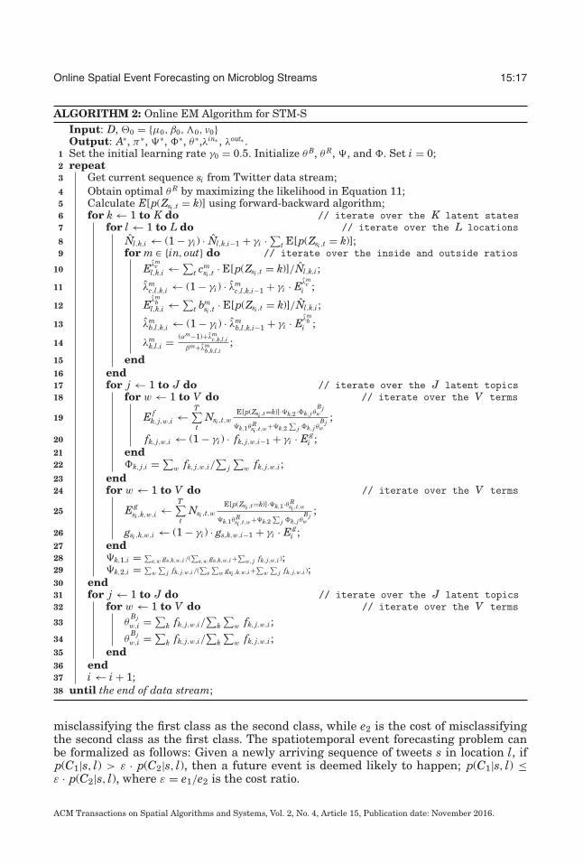
online spatial event forecasting in microblogs -...
TRANSCRIPT
15
Online Spatial Event Forecasting in Microblogs
LIANG ZHAO, George Mason UniversityFENG CHEN, University of Albany, SUNYCHANG-TIEN LU and NAREN RAMAKRISHNAN, Virginia Tech
Event forecasting from social media data streams has many applications. Existing approaches focus onforecasting temporal events (such as elections and sports) but as yet cannot forecast spatiotemporal eventssuch as civil unrest and influenza outbreaks, which are much more challenging. To achieve spatiotemporalevent forecasting, spatial features that evolve with time and their underlying correlations need to be con-sidered and characterized. In this article, we propose novel batch and online approaches for spatiotemporalevent forecasting in social media such as Twitter. Our models characterize the underlying developmentof future events by simultaneously modeling the structural contexts and their spatiotemporal burstinessbased on different strategies. Both batch and online-based inference algorithms are developed to optimizethe model parameters. Utilizing the trained model, the alignment likelihood of tweet sequences is calculatedby dynamic programming. Extensive experimental evaluations on two different domains demonstrate theeffectiveness of our proposed approach.
CCS Concepts: � Computing methodologies → Bayesian network models
Additional Key Words and Phrases: Graphical models, spatiotemporal event forecasting, social media
ACM Reference Format:Liang Zhao, Feng Chen, Chang-Tien Lu, and Naren Ramakrishnan. 2016. Online spatial event forecastingin microblogs. ACM Trans. Spatial Algorithms Syst. 2, 4, Article 15 (November 2016), 39 pages.DOI: http://dx.doi.org/10.1145/2997642
1. INTRODUCTION
Microblogs like Twitter and Weibo are important platforms for ongoing discussionsof societal events [Kwak et al. 2010]. As of the end of 2014, 255 million active userswere collectively creating 500 million tweets every day, covering a whole varietyof content ranging from everyday feelings to comments about social gatherings[Bennett 2014]. Compared to traditional media, Twitter has the following significantcharacteristics: (i) Timeliness of messages: Unlike traditional media, which may takehours or days to publish information, tweets can be posted instantly utilizing portablemobile devices in users’ pockets; 2 = (ii) ubiquity of social sensors: tweets reflect thepublic’s mood and trends, both of which are potential determinants of future socialevents; and (iii) availability of geo-information: Twitter users provide rich locationinformation within their profiles, texts, and geotags. Recent research has revealedthe power of Twitter for event forecasting [Tumasjan et al. 2010; Wang et al. 2012b];Twitter and other social media have been recognized as playing a key role in events
Authors’ addresses: L. Zhao, 12566 Summit Manor Drive # 224, Fairfax, VA 22033; email: [email protected];F. Chen, LI-96J, 1400 Washington Avenue, Albany, NY 12222; email: [email protected]; C.-T. Lu, 7054Haycock Road, Falls Church, VA 22043; email: [email protected]; N. Ramakrishnan, 7054 Haycock Road, FallsChurch, VA 22043; email: [email protected] to make digital or hard copies of part or all of this work for personal or classroom use is grantedwithout fee provided that copies are not made or distributed for profit or commercial advantage and thatcopies show this notice on the first page or initial screen of a display along with the full citation. Copyrights forcomponents of this work owned by others than ACM must be honored. Abstracting with credit is permitted.To copy otherwise, to republish, to post on servers, to redistribute to lists, or to use any component of thiswork in other works requires prior specific permission and/or a fee. Permissions may be requested fromPublications Dept., ACM, Inc., 2 Penn Plaza, Suite 701, New York, NY 10121-0701 USA, fax +1 (212)869-0481, or [email protected]© 2016 ACM 2374-0353/2016/11-ART15 $15.00DOI: http://dx.doi.org/10.1145/2997642
ACM Transactions on Spatial Algorithms and Systems, Vol. 2, No. 4, Article 15, Publication date: November 2016.
15:2 L. Zhao et al.
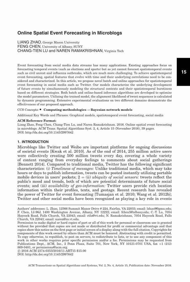
Fig. 1. Twitter predicts a presidential election protest.
such as the “Arab Spring” and the protests surrounding the Mexican presidentialelection [Ramakrishnan et al. 2014; Wang et al. 2012b]. Figure 1 depicts the activitieson Twitter that causally preceded the Mexico City protests. Both the content andthe spatiotemporal burstiness of these protest-related tweets reveal the escalation ofsocietal discontent pertaining to this controversial election, with users progressingfrom complaining through planning and advertising to participating in the finalprotest event. However, existing event forecasting models in Twitter generally focuson temporal events whose geo-locations are not available or are not considered in theprediction task (e.g., elections [Tumasjan et al. 2010] and sports [Pavlyshenko 2013]).Comparatively little attention has been paid to forecasting spatiotemporal events.
Tweets posted within a certain geographical neighborhood could be able to reflect im-portant spatiotemporal patterns of social event [Zhao et al. 2014]. Thus, the forecastingof spatiotemporal events requires a consideration of spatial features and their correla-tions in addition to the temporal dimension. This poses the following three challenges:(i) Capturing spatiotemporal dependencies. A spatial event may be delineated by notonly a specific location and time, but also its geographical and temporal neighborhood.The strength and pattern of the resulting tweets may also vary differently for differentdevelopment stages for different events. (ii) Modeling mixed type observations. Whenan event occurs, this will involve the temporal evolution of spatially distributed tweetsdescribing the event and its semantics. The joint consideration of these heterogeneousand multidimensional data points is thus crucial. And (iii), utilizing prior geographi-cal knowledge. Spatiotemporal events in crucial domains usually have rich historical
ACM Transactions on Spatial Algorithms and Systems, Vol. 2, No. 4, Article 15, Publication date: November 2016.
Online Spatial Event Forecasting on Microblog Streams 15:3
records. Different geo-locations may tend to feature their own inherent and distinctevent frequencies that can be integrated into a predictive model to improve the fore-casting accuracy. For example, the historical crime rates in different areas of a city canhelp forecast the probability of future crimes occurring in those areas.
This article proposes a new approach to developing spatiotemporal event forecast-ing models that addresses the above-mentioned issues more effectively. The proposedmethodology generatively characterizes the evolutionary development of events, aswell as the relationships between the tweet observations both inside and outside theevent venue. To uncover the underlying event development mechanics, this approachjointly considers the structural semantics and spatial-temporal burstiness patterns inTwitter streams. Utilizing geographical priors allows the spatial burstiness distribu-tions to be learned for specific corresponding locations, while applying a Gaussian-inverse Wishart prior distribution facilitates event forecasting for unknown locations.The main contributions of this article are:
—A novel generative framework for spatial event forecasting. For spatial eventforecasting in Twitter, we propose an enhanced Hidden Markov Model (HMM) thatcharacterizes the transitional process of event development by jointly consideringthe time-evolving context and space-time burstiness of Twitter streams.
—Effective batch and online algorithms for model parameter inference. Themodel inference is formalized as the maximization of a posterior that is analyticallytractable. Both Expectation Maximization (EM)-based and stochastic-EM parameteroptimization algorithms are proposed to solve this problem effectively and efficiently.
—A new sequence likelihood calculation method. To handle the noisy nature oftweet content, words that are exclusive to a single event are identified by a languagemodel that has been optimized by a dynamic programming algorithm to achieve anaccurate sequence likelihood calculation.
—Extensive experimental performance evaluations. The proposed method out-performs existing methods by 38% and 67% on two different real-world datasets.Sensitivity analyses reveal the impact of the parameters on the new method’s perfor-mance. Case studies on both datasets are illustrated and elaborated to demonstratethe practical utility of the proposed methods.
The rest of this article is organized as follows. Section 2 reviews existing work inthis area, after which Section 3 describes the proposed generative model, Section 4provides details of the associated parameter estimation, and Section 5 explains theevent forecasting function of the proposed model. In Section 6, extensive experimentsto evaluate the performance of the new model are conducted and analyzed; the work issummarized and conclusions drawn in Section 7.
2. RELATED WORK
Current research into the analysis of Twitter-based social events can be categorizedinto two main types: (i) event detection and (ii) event forecasting. These are consideredin turn here.
Event detection: A large body of work focuses on the detection of ongoing events[Aggarwal and Subbian 2012; Lappas et al. 2012; Sakaki et al. 2010; Signorini et al.2011; Weng and Lee 2011]. These papers treat tweets as real-time social sensors topromptly discover new events as they occur. Methods based on spatial bursts use aclassifier to extract topic-related tweets and then examine their spatial burstinessand have been tested for applications such as detecting earthquakes [Sakaki et al.2010] and disease outbreaks [Signorini et al. 2011], while methods based on temporalbursts detect temporal patterns in Twitter streams utilizing techniques such as waveletanalysis [Weng and Lee 2011], temporal clustering [Aggarwal and Subbian 2012], and
ACM Transactions on Spatial Algorithms and Systems, Vol. 2, No. 4, Article 15, Publication date: November 2016.
15:4 L. Zhao et al.
query expansion [Zhao et al. 2015a; Jin et al. 2014]. Existing methods developed forflu detection are typically focused on the temporal dimension. For example, Ginsberget al. proposed monitoring ongoing flu activity using Google search engine data. Incontrast, spatiotemporal methods aim to detect bursts in both time and space [Ginsberget al. 2009]. However, these event detection approaches can only uncover events afterthey have occurred and are unable to forecast future events because they focus onobservations that directly reflect currently occurring events rather than precursorindicators that reveal the causes or development of future events.
Event forecasting: Most research in this area focuses on temporal events and ig-nores the underlying geographical information that is also available in tweets. A varietyof applications have been explored, including predicting election outcomes [O’Connoret al. 2010; Tumasjan et al. 2010], disease outbreaks [Achrekar et al. 2011; Rittermanet al. 2009; Zhao et al. 2016], stock market movements [Arias et al. 2013; Bollen et al.2011], politics [Marchetti-Bowick and Chambers 2012], box office ticket sales [Ariaset al. 2013], the Olympic games [Pavlyshenko 2013], crime [Wang et al. 2012b], andtraffic conditions [He et al. 2013]. These papers can be categorized into four typesbased on the complexity of the models utilized: (i) Linear regression models. Thesemethods map simple predictive features such as sentiment score or tweet volume tothe occurrence of future events [Arias et al. 2013; Bollen et al. 2011; He et al. 2013;O’Connor et al. 2010]. (ii) Nonlinear models. These methods incorporate more infor-mative features such as semantic topics by utilizing methods such as support vectormachines and logistic regression [Ritterman et al. 2009; Wang et al. 2012b]. (iii) Timeseries-based methods. These methods consider the temporal correlation of relevantfeatures such as tweet volume by adopting approaches such as autoregressive model-ing. For example, Achrekar et al. [2011] utilize an autoregression with exogenous input(ARX) model to forecast flu activity over the next few days. And (iv) domain-specificapproaches. These methods are designed to solve particular problems and may notbe applicable to other application domains. For example, Pavlyshenko [2013] appliedan association rule approach to discover the most frequently mentioned players andhence predict the results of sports tournaments, while Marchetti-Bowick and Chambers[2012] focused on improving the performance of sentiment analysis related to politi-cal events. As yet, there have been few reports of work specifically on spatiotemporalevent forecasting. Gerber [2014] proposed a predictor for spatiotemporal events thatutilized historical event counts and topics but did not consider temporal evolution anddependencies, while Wang et al. [2012a] developed a model to characterize and predictspatiotemporal criminal incidents, although their model requires the availability of de-mographic information. Zhao et al. [2015b] proposed three multitask learning modelsto forecast civil unrest events utilizing static features and dynamic features. Insteadof considering geographic neighborhoods, these models assume all the locations in acountry interact equally with each other.
This article proposes a spatiotemporal event forecasting method that is capableof characterizing the evolutionary pattern of both spatial burstiness and structuralcontexts. By modeling geographical priors more effectively, the new approach proposedhere can sufficiently leverage historical prior knowledge for it to be applied to newlocations.
3. GENERATIVE PROCESS OF THE PROPOSED MODELS
This section describes the formulation and generative process of the proposed methods.First, the spatiotemporal event forecasting problem is formalized; then our new gener-ative model is described in detail, including the space-time burstiness and structuraltweet content modules.
ACM Transactions on Spatial Algorithms and Systems, Vol. 2, No. 4, Article 15, Publication date: November 2016.
Online Spatial Event Forecasting on Microblog Streams 15:5
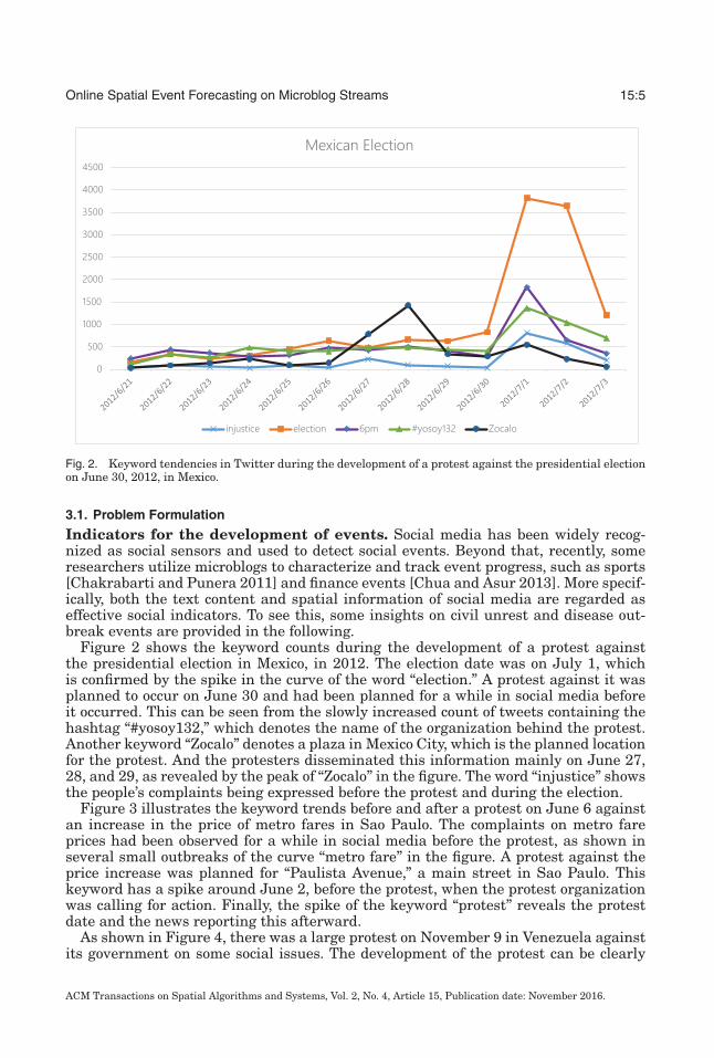
Fig. 2. Keyword tendencies in Twitter during the development of a protest against the presidential electionon June 30, 2012, in Mexico.
3.1. Problem Formulation
Indicators for the development of events. Social media has been widely recog-nized as social sensors and used to detect social events. Beyond that, recently, someresearchers utilize microblogs to characterize and track event progress, such as sports[Chakrabarti and Punera 2011] and finance events [Chua and Asur 2013]. More specif-ically, both the text content and spatial information of social media are regarded aseffective social indicators. To see this, some insights on civil unrest and disease out-break events are provided in the following.
Figure 2 shows the keyword counts during the development of a protest againstthe presidential election in Mexico, in 2012. The election date was on July 1, whichis confirmed by the spike in the curve of the word “election.” A protest against it wasplanned to occur on June 30 and had been planned for a while in social media beforeit occurred. This can be seen from the slowly increased count of tweets containing thehashtag “#yosoy132,” which denotes the name of the organization behind the protest.Another keyword “Zocalo” denotes a plaza in Mexico City, which is the planned locationfor the protest. And the protesters disseminated this information mainly on June 27,28, and 29, as revealed by the peak of “Zocalo” in the figure. The word “injustice” showsthe people’s complaints being expressed before the protest and during the election.
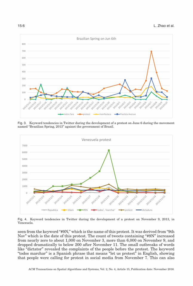
Figure 3 illustrates the keyword trends before and after a protest on June 6 againstan increase in the price of metro fares in Sao Paulo. The complaints on metro fareprices had been observed for a while in social media before the protest, as shown inseveral small outbreaks of the curve “metro fare” in the figure. A protest against theprice increase was planned for “Paulista Avenue,” a main street in Sao Paulo. Thiskeyword has a spike around June 2, before the protest, when the protest organizationwas calling for action. Finally, the spike of the keyword “protest” reveals the protestdate and the news reporting this afterward.
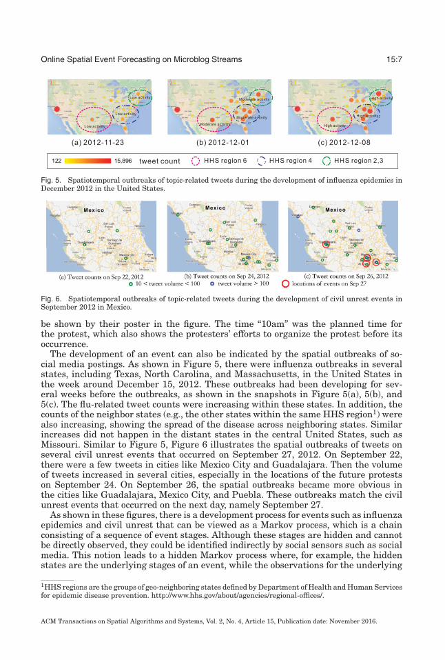
As shown in Figure 4, there was a large protest on November 9 in Venezuela againstits government on some social issues. The development of the protest can be clearly
ACM Transactions on Spatial Algorithms and Systems, Vol. 2, No. 4, Article 15, Publication date: November 2016.
15:6 L. Zhao et al.
Fig. 3. Keyword tendencies in Twitter during the development of a protest on June 6 during the movementnamed “Brazilian Spring, 2013” against the government of Brazil.
Fig. 4. Keyword tendencies in Twitter during the development of a protest on November 9, 2013, inVenezuela.
seen from the keyword “#9N,” which is the name of this protest. It was derived from “9thNov” which is the date of this protest. The count of tweets containing “#9N” increasedfrom nearly zero to about 1,000 on November 3, more than 6,000 on November 9, anddropped dramatically to below 200 after November 11. The small outbreaks of wordslike “dictator” revealed the complaints of the people before the protest. The keyword“todos marchar” is a Spanish phrase that means “let us protest” in English, showingthat people were calling for protest in social media from November 7. This can also
ACM Transactions on Spatial Algorithms and Systems, Vol. 2, No. 4, Article 15, Publication date: November 2016.
Online Spatial Event Forecasting on Microblog Streams 15:7
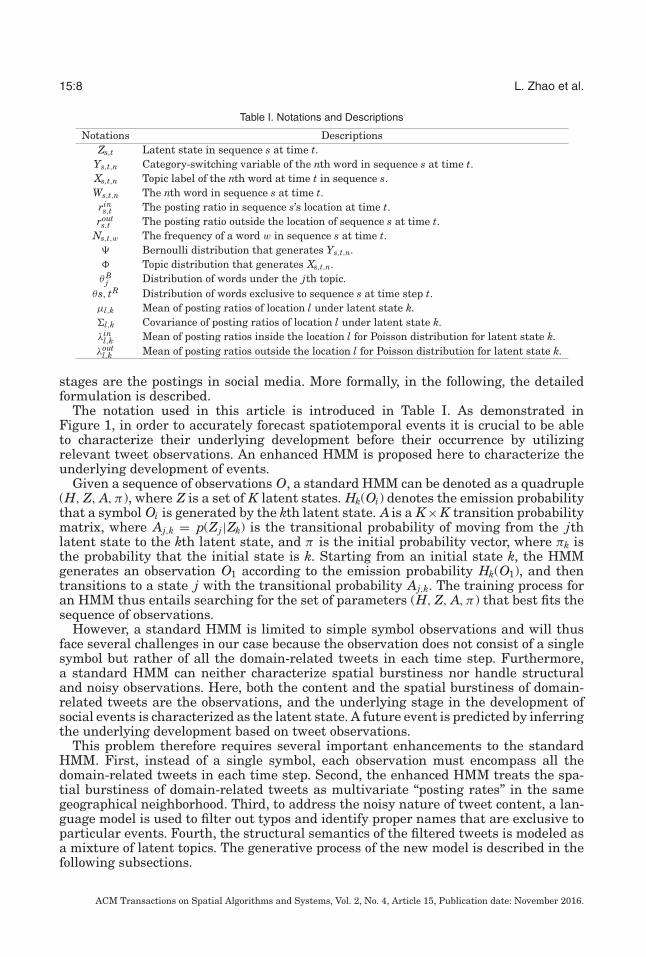
Fig. 5. Spatiotemporal outbreaks of topic-related tweets during the development of influenza epidemics inDecember 2012 in the United States.
Fig. 6. Spatiotemporal outbreaks of topic-related tweets during the development of civil unrest events inSeptember 2012 in Mexico.
be shown by their poster in the figure. The time “10am” was the planned time forthe protest, which also shows the protesters’ efforts to organize the protest before itsoccurrence.
The development of an event can also be indicated by the spatial outbreaks of so-cial media postings. As shown in Figure 5, there were influenza outbreaks in severalstates, including Texas, North Carolina, and Massachusetts, in the United States inthe week around December 15, 2012. These outbreaks had been developing for sev-eral weeks before the outbreaks, as shown in the snapshots in Figure 5(a), 5(b), and5(c). The flu-related tweet counts were increasing within these states. In addition, thecounts of the neighbor states (e.g., the other states within the same HHS region1) werealso increasing, showing the spread of the disease across neighboring states. Similarincreases did not happen in the distant states in the central United States, such asMissouri. Similar to Figure 5, Figure 6 illustrates the spatial outbreaks of tweets onseveral civil unrest events that occurred on September 27, 2012. On September 22,there were a few tweets in cities like Mexico City and Guadalajara. Then the volumeof tweets increased in several cities, especially in the locations of the future protestson September 24. On September 26, the spatial outbreaks became more obvious inthe cities like Guadalajara, Mexico City, and Puebla. These outbreaks match the civilunrest events that occurred on the next day, namely September 27.
As shown in these figures, there is a development process for events such as influenzaepidemics and civil unrest that can be viewed as a Markov process, which is a chainconsisting of a sequence of event stages. Although these stages are hidden and cannotbe directly observed, they could be identified indirectly by social sensors such as socialmedia. This notion leads to a hidden Markov process where, for example, the hiddenstates are the underlying stages of an event, while the observations for the underlying
1HHS regions are the groups of geo-neighboring states defined by Department of Health and Human Servicesfor epidemic disease prevention. http://www.hhs.gov/about/agencies/regional-offices/.
ACM Transactions on Spatial Algorithms and Systems, Vol. 2, No. 4, Article 15, Publication date: November 2016.
15:8 L. Zhao et al.
Table I. Notations and Descriptions
Notations DescriptionsZs,t Latent state in sequence s at time t.
Ys,t,n Category-switching variable of the nth word in sequence s at time t.Xs,t,n Topic label of the nth word at time t in sequence s.Ws,t,n The nth word in sequence s at time t.rins,t The posting ratio in sequence s’s location at time t.
routs,t The posting ratio outside the location of sequence s at time t.
Ns,t,w The frequency of a word w in sequence s at time t.� Bernoulli distribution that generates Ys,t,n.� Topic distribution that generates Xs,t,n.θ B
j Distribution of words under the jth topic.θs, tR Distribution of words exclusive to sequence s at time step t.μl,k Mean of posting ratios of location l under latent state k.�l,k Covariance of posting ratios of location l under latent state k.λin
l,k Mean of posting ratios inside the location l for Poisson distribution for latent state k.λout
l,k Mean of posting ratios outside the location l for Poisson distribution for latent state k.
stages are the postings in social media. More formally, in the following, the detailedformulation is described.
The notation used in this article is introduced in Table I. As demonstrated inFigure 1, in order to accurately forecast spatiotemporal events it is crucial to be ableto characterize their underlying development before their occurrence by utilizingrelevant tweet observations. An enhanced HMM is proposed here to characterize theunderlying development of events.
Given a sequence of observations O, a standard HMM can be denoted as a quadruple(H, Z, A, π ), where Z is a set of K latent states. Hk(Oi) denotes the emission probabilitythat a symbol Oi is generated by the kth latent state. A is a K× K transition probabilitymatrix, where Aj,k = p(Zj |Zk) is the transitional probability of moving from the jthlatent state to the kth latent state, and π is the initial probability vector, where πk isthe probability that the initial state is k. Starting from an initial state k, the HMMgenerates an observation O1 according to the emission probability Hk(O1), and thentransitions to a state j with the transitional probability Aj,k. The training process foran HMM thus entails searching for the set of parameters (H, Z, A, π ) that best fits thesequence of observations.
However, a standard HMM is limited to simple symbol observations and will thusface several challenges in our case because the observation does not consist of a singlesymbol but rather of all the domain-related tweets in each time step. Furthermore,a standard HMM can neither characterize spatial burstiness nor handle structuraland noisy observations. Here, both the content and the spatial burstiness of domain-related tweets are the observations, and the underlying stage in the development ofsocial events is characterized as the latent state. A future event is predicted by inferringthe underlying development based on tweet observations.
This problem therefore requires several important enhancements to the standardHMM. First, instead of a single symbol, each observation must encompass all thedomain-related tweets in each time step. Second, the enhanced HMM treats the spa-tial burstiness of domain-related tweets as multivariate “posting rates” in the samegeographical neighborhood. Third, to address the noisy nature of tweet content, a lan-guage model is used to filter out typos and identify proper names that are exclusive toparticular events. Fourth, the structural semantics of the filtered tweets is modeled asa mixture of latent topics. The generative process of the new model is described in thefollowing subsections.
ACM Transactions on Spatial Algorithms and Systems, Vol. 2, No. 4, Article 15, Publication date: November 2016.
Online Spatial Event Forecasting on Microblog Streams 15:9
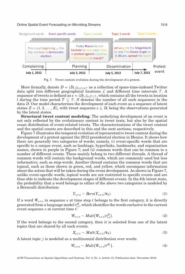
Fig. 7. Tweet context evolution during the development of a protest.
More formally, denote D = {Dl,t}l∈L,t∈T as a collection of space-time-indexed Twitterdata split into different geographical locations L and different time intervals T . Asequence of tweets is defined as s = {Dl,t}t∈T ⊆T , which contains all the tweets in locationl during the time period T ⊆ T . S denotes the number of all such sequences in thedata D. Our model characterizes the development of each event as a sequence of latentstates Z = {1, 2, . . . , K}, with tweet sequence s ⊆ Dl being the observations generatedby the latent states.
Structural tweet content modeling. The underlying development of an event isnot only reflected by the evolutionary content in tweet texts, but also by the spatialcount distribution of event-related tweets. The characterizations of the tweet contentand the spatial counts are described in this and the next sections, respectively.
Figure 7 illustrates the temporal evolution of representative tweet content during thedevelopment of a protest against the 2012 presidential election in Mexico. It shows howthere are generally two categories of words; namely, (i) event-specific words that arespecific to a unique event, such as hashtags, hyperlinks, landmarks, and organizationnames, shown in purple in Figure 7; and (ii) common words that can be common to anumber of different events. These mainly belong to two different threads. A thread ofcommon words will contain the background words, which are commonly used but lessinformative, such as stop-words. Another thread contains the common words that aretopical, such as those shown in green, red, and yellow, which encompass informationabout the action that will be taken during the event development. As shown in Figure 7,unlike event-specific words, topical words are not restricted to specific events and arethus able to indicate the development stages of different events. In the kth latent state,the probability that a word belongs to either of the above two categories is modeled bya Bernoulli distribution:
Ys,t,n ∼ Bern(Ys,t,n|�k). (1)
If a word Ws,t,n in sequence s at time step t belongs to the first category, it is directlygenerated from a language model θ R
s,t, which identifies the words exclusive to the currentevent sequence s at current time t:
Ws,t,n ∼ Mult(Ws,t,n|θ R
s,t
). (2)
If the word belongs to the second category, then it is selected from one of the latenttopics that are shared by all such events.
Xs,t,n ∼ Mult(Xs,t,n|�k). (3)
A latent topic j is modeled as a multinomial distribution over words:
Ws,t,n ∼ Mult(Ws,t,n|θ Bj
). (4)
ACM Transactions on Spatial Algorithms and Systems, Vol. 2, No. 4, Article 15, Publication date: November 2016.
15:10 L. Zhao et al.
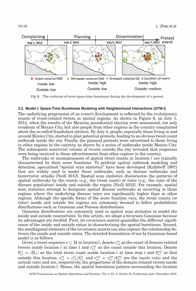
Fig. 8. The evolution of tweet space-time burstiness during the development of a protest.
3.2. Model I: Space-Time Burstiness Modeling with Neighborhood Interactions (STM-I)
The underlying progression of an event’s development is reflected by the evolutionarycounts of event-related tweets in spatial regions. As shown in Figure 8, on July 1,2012, when the results of the Mexican presidential election were announced, not onlyresidents of Mexico City, but also people from other regions in the country complainedabout the so-called fraudulent election. By July 4, people, especially those living in andaround Mexico City, started to plan potential protests, leading to an obvious tweet countoutbreak inside the city. Finally, the planned protests were advertised to those livingin other regions in the country, as shown by a series of outbreaks inside Mexico City.The subsequent nontrivial volume of tweets outside the city revealed that responseswere being received to these advertisement from other regions in the country.
The outbreaks or anomalousness of spatial tweet counts in location l are typicallycharacterized by their score functions. To perform spatial outbreak modeling anddetection, specialized “spatial scan statistics” have been developed [Kulldorff 1997]that are widely used to model these outbreaks, such as disease outbreaks andbioterrorist attacks [Neill 2012]. Spatial scan statistics characterize the patterns ofspatial outbreaks by the counts (e.g., the tweet count) or rates (e.g., the ratio of thedisease population) inside and outside the region [Neill 2012]. For example, spatialscan statistics attempt to designate spatial disease outbreaks as occurring in thoseregions where the underlying disease rates are significantly higher than in otherregions. Although the specific forms of the score function vary, the tweet counts (orrates) inside and outside the regions are commonly deemed to follow probabilisticdistributions such as Gaussian and Poisson distributions.
Gaussian distributions are commonly used in spatial scan statistics to model theinside and outside counts/rates. In this article, we adopt a bivariate Gaussian becauseits advantages are twofold. First, its covariance matrix quantifies the different signifi-cance of the inside and outside ratios in characterizing the spatial burstiness. Second,the nondiagonal elements of the covariance matrix can also capture the relationship be-tween the inside and outside ratios. The detailed formulation of our bi-Gaussian-basedmodel is as follows.
Given a tweet sequence s ⊆ Dl in location l, denote cins,t as the count of domain-related
tweets inside location l at time t and couts,t as the count outside this location. Denote
bins,t = |Dl,t| as the total tweet count inside location l at time step t and bout
s,t as thatoutside this location. rin
s,t = cins,t/bin
s,t and routs,t = cout
s,t /bouts,t are the inside ratio and the
outside ratio and are, respectively, the proportions of the domain-related tweets insideand outside location l. Hence, the spatial burstiness pattern surrounding the location
ACM Transactions on Spatial Algorithms and Systems, Vol. 2, No. 4, Article 15, Publication date: November 2016.
Online Spatial Event Forecasting on Microblog Streams 15:11
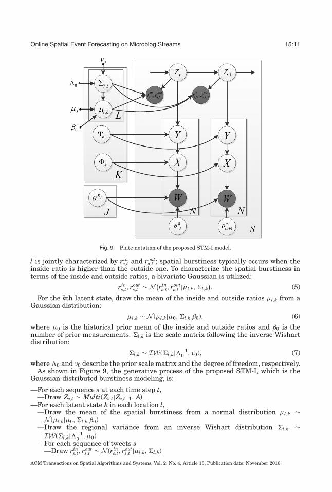
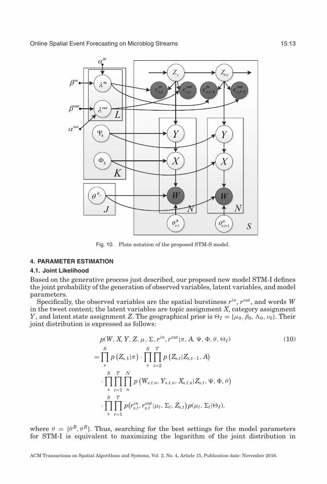
Fig. 9. Plate notation of the proposed STM-I model.
l is jointly characterized by rins,t and rout
s,t ; spatial burstiness typically occurs when theinside ratio is higher than the outside one. To characterize the spatial burstiness interms of the inside and outside ratios, a bivariate Gaussian is utilized:
rins,t, rout
s,t ∼ N(rin
s,t, routs,t |μl,k, �l,k
). (5)
For the kth latent state, draw the mean of the inside and outside ratios μl,k from aGaussian distribution:
μl,k ∼ N (μl,k|μ0, �l,k β0), (6)
where μ0 is the historical prior mean of the inside and outside ratios and β0 is thenumber of prior measurements. �l,k is the scale matrix following the inverse Wishartdistribution:
�l,k ∼ IW(�l,k|−10 , ν0), (7)
where 0 and ν0 describe the prior scale matrix and the degree of freedom, respectively.As shown in Figure 9, the generative process of the proposed STM-I, which is the
Gaussian-distributed burstiness modeling, is:
—For each sequence s at each time step t,—Draw Zs,t ∼ Multi(Zs,t|Zs,t−1, A)
—For each latent state k in each location l,—Draw the mean of the spatial burstiness from a normal distribution μl,k ∼
N (μl,k|μ0, �l,k β0)—Draw the regional variance from an inverse Wishart distribution �l,k ∼
IW(�l,k|−10 , μ0)
—For each sequence of tweets s—Draw rin
s,t, routs,t ∼ N (rin
s,t, routs,t |μl,k, �l,k)
ACM Transactions on Spatial Algorithms and Systems, Vol. 2, No. 4, Article 15, Publication date: November 2016.
15:12 L. Zhao et al.
—For each word Wn in time step t in tweet sequence s,—Draw Ys,t,n ∼ Bern(Ys,t,n|�k)—If Ys,t,n = 0, draw Ws,t,n ∼ Mult(Ws,t,n|θ R
s,t)—else
—Draw a topic Xs,t,n ∼ Mult(Xs,t,n|�k).—Draw a word Ws,t,n ∼ Mult(Ws,t,n|θ Bj , j = Xs,t,n).
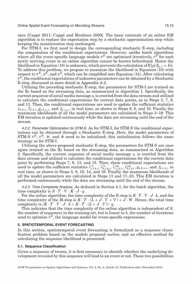
3.3. Model II: Space-Time Burstiness with Non-negative-Discrete Signals
The model in the previous section, STM-I, characterizes the space-time burstiness bynot only considering the signal strengths at different locations, but also the poten-tial correlations among these locations by leveraging the covariance. In spite of theseadvantages, however, important signals such as the volume of tweets are typically non-negative and discrete and are thus not naturally handled by a Gaussian distribution.To address this issue, in addition to the Gaussian-based version just described, wepropose another model, STM-S, to preserve these non-negative and discrete propertiesbased on a Poisson distribution. Specifically, the counts cin
s,t and couts,t are assumed to be
Poisson distributed and designated as follows:cin
s,t ∼ Poisson(cin
s,t|λink,l · bin
s,t
),
couts,t ∼ Poisson
(cout
s,t |λoutk,l · bout
s,t
), (8)
where bins,t and bout
s,t , as previously, represent the total tweet count inside and outsidelocation l at time step t, respectively, and λin
k,l and λoutk,l denote the means of the inside
and outside outbreak ratios, respectively.Prior knowledge of sufficient statistics to permit a Poisson distribution for different
locations and different states follows Gamma distributions:λin
k,l ∼ Gamma(λin
k,l|αin, βin),λout
k,l ∼ Gamma(λout
k,l |αout, βout), (9)
where αin and βin denote the shape parameter and inverse scale parameter of theGamma prior for the inside outbreaks distribution. αout and βout denote the shapeparameter and inverse scale parameter of the Gamma prior for the outside outbreaksdistribution.
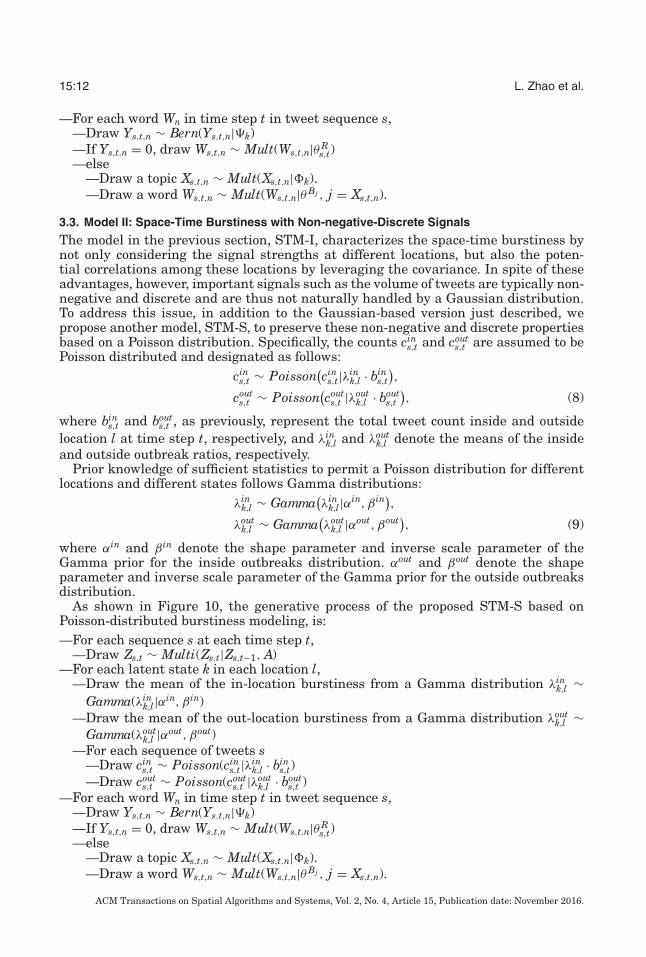
As shown in Figure 10, the generative process of the proposed STM-S based onPoisson-distributed burstiness modeling, is:—For each sequence s at each time step t,
—Draw Zs,t ∼ Multi(Zs,t|Zs,t−1, A)—For each latent state k in each location l,
—Draw the mean of the in-location burstiness from a Gamma distribution λink,l ∼
Gamma(λink,l|αin, βin)
—Draw the mean of the out-location burstiness from a Gamma distribution λoutk,l ∼
Gamma(λoutk,l |αout, βout)
—For each sequence of tweets s—Draw cin
s,t ∼ Poisson(cins,t|λin
k,l · bins,t)
—Draw couts,t ∼ Poisson(cout
s,t |λoutk,l · bout
s,t )—For each word Wn in time step t in tweet sequence s,
—Draw Ys,t,n ∼ Bern(Ys,t,n|�k)—If Ys,t,n = 0, draw Ws,t,n ∼ Mult(Ws,t,n|θ R
s,t)—else
—Draw a topic Xs,t,n ∼ Mult(Xs,t,n|�k).—Draw a word Ws,t,n ∼ Mult(Ws,t,n|θ Bj , j = Xs,t,n).
ACM Transactions on Spatial Algorithms and Systems, Vol. 2, No. 4, Article 15, Publication date: November 2016.
Online Spatial Event Forecasting on Microblog Streams 15:13
Fig. 10. Plate notation of the proposed STM-S model.
4. PARAMETER ESTIMATION
4.1. Joint Likelihood
Based on the generative process just described, our proposed new model STM-I definesthe joint probability of the generation of observed variables, latent variables, and modelparameters.
Specifically, the observed variables are the spatial burstiness rin, rout, and words Win the tweet content; the latent variables are topic assignment X, category assignmentY , and latent state assignment Z. The geographical prior is �I = {μ0, β0,0, ν0}. Theirjoint distribution is expressed as follows:
p(W, X, Y, Z, μ,�, rin, rout|π, A, �,�, θ,�I) (10)
=S∏s
p(Zs,1|π
) ·S∏s
T∏t=2
p(Zs,t|Zs,t−1, A
)
·S∏s
T∏t=1
N∏n
p(Ws,t,n, Ys,t,n, Xs,t,n|Zs,t, �,�, θ
)
·S∏s
T∏t=1
p(rin
s,t, routs,t |μl, �l, Zs,t
)p(μl, �l|�I),
where θ = {θ B, θ R}. Thus, searching for the best settings for the model parametersfor STM-I is equivalent to maximizing the logarithm of the joint distribution in
ACM Transactions on Spatial Algorithms and Systems, Vol. 2, No. 4, Article 15, Publication date: November 2016.
15:14 L. Zhao et al.
Equation (10). The specific optimization process of this objective function is listed inEquations (18–22) and Equations (29–36) in Appendix A.1.
In STM-S, the Poisson-distributed space-time burstiness modeling approach meansthat the observed variables are the inside domain-related tweet counts cin, the insidebase counts bin, the outside domain-related tweet counts cout, the outside base countsbout, and the words W in the tweet content; the latent variables are once again topicassignment X, category assignment Y , and latent state assignment Z. The geographicalprior is �II = {αin, βin, αout, βout}. The joint distribution is expressed as follows:
p(W, X, Y, Z, μ,�, rin, rout|π, A, �,�, θ,�IIch) (11)
=S∏s
p(Zs,1|π
) ·S∏s
T∏t=2
p(Zs,t|Zs,t−1, A
)
·S∏s
T∏t=1
N∏n
p(Ws,t,n, Ys,t,n, Xs,t,n|Zs,t, �,�, θ
)
·S∏s
T∏t=1
p(cin
s,t|bins,t · λin
l
) · p(cout
s,t |bins,t · λin
l
)
· p(λin
l , λoutl |�II
).
Thus, searching for the best set of model parameters for STM-S is equivalent to maxi-mizing the logarithm of the joint distribution in Equation (11). The specific optimizationprocess of this objective function is listed in Equations (18, 23–36) in Appendix A.1.
Utilizing the prior distributions �I and �II enables the model to estimate the spatialburstiness distribution even when there are no spatial outbreak observations. Thisadvantage makes it possible to conduct event predictions even in new locations. Morespecifically for the model STM-I, according to Equation (19) in Appendix A.1, when(rin
s,t, routs,t ) is not available, then μl,k = 0. Therefore, μl,k = μ0 according to Equation (21).
For STM-S, which utilizes a Poisson distribution, the deduction is the same, usingEquations (27) and (28).
The time consumption required by the preceding algorithm is composed of two parts:(i) the computation of the forward-backward algorithm and (ii) the computation ofEquations (18)–(36). The time complexity of the first of these is S · T · K, where S isthe number of sequences, T is the time length of a sequence, and K is the number oflatent states. The time complexity of the second is S · T · V · K + S · T · V · K · J, whereN is the size of the vocabulary and J is the number of latent topics. Combining the twoparts and multiplying the result by the number of EM iterations q, the comprehensivetime complexity, is S · T · V · K · J · q.
Given the large numerical value of S, which includes all the historical sequences,the batch EM algorithm for estimating the model parameters is inevitably quite time-consuming. Moreover, as Twitter streams in real time, the batch-based updating of themodel parameter to cope with the constant flow of incoming data requires the continualrecalculation of the entire historical training set, which is prohibitively expensive inpractice. To address this issue, we propose the use of an online parameter optimizationmethod, which is introduced in the following section.
4.2. Online Parameter Optimization Algorithm
This section proposes online parameter optimization algorithms for STM-I and STM-S.
4.2.1. Parameter Optimization for STM-I. Unlike a standard batch EM algorithm, the ca-pacity to perform online estimation means that the data must be run through only
ACM Transactions on Spatial Algorithms and Systems, Vol. 2, No. 4, Article 15, Publication date: November 2016.
Online Spatial Event Forecasting on Microblog Streams 15:15
once [Cappe 2011; Cappe and Moulines 2009]. The basic rationale of an online EMalgorithm is to replace the expectation step by a stochastic approximation step whilekeeping the maximization step unchanged.
For STM-I, we first need to design the corresponding stochastic E-step, includingthe computation of the conditional expectations. However, unlike batch algorithmswhere all the event-specific language models θ R are optimized iteratively, θ R for eachnewly arriving event in an online algorithm cannot be known beforehand. Hence thelikelihood in Equation (10) is unknown, which prevents the calculation of E[p(Zsi ,t = k)].To address this problem, we propose to maximize the likelihood in Equation (10) withrespect to θ R, nR, and nB, which can be simplified into Equation (14). After calculatingθ R, the conditional expectations of unknown parameters can be obtained by a StochasticE-step, discussed in more detail in Appendix A.2.
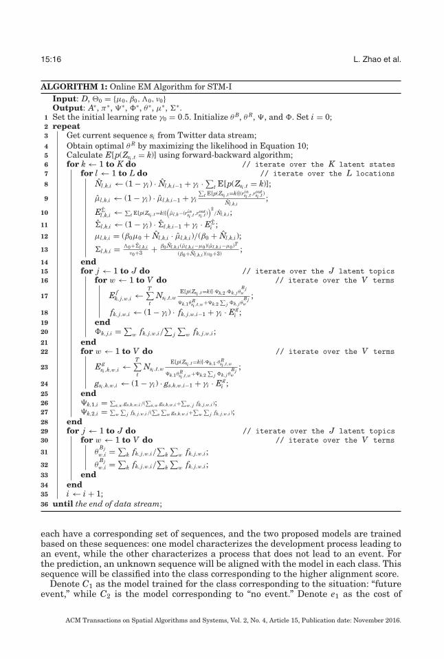
Utilizing the preceding stochastic E-step, the parameters for STM-I are trained onthe fly based on the streaming data, as summarized in Algorithm 1. Specifically, thecurrent sequence of social media message si is crawled from the data stream and utilizedto calculate the conditional expectations for current data points, as in Steps 5, 7, 9,and 11. Then, the conditional expectations are used to update the sufficient statisticsμl,k,i, �l,k,i, gs,k,w,i, and fk, j,w,i in real time, as shown in Steps 6, 8, and 10. Finally, themaximum likelihoods of all the model parameters are calculated in Steps 3–19. ThisEM iteration is updated continuously while the data are streaming until the end of thestream.
4.2.2. Parameter Optimization for STM-S. As for STM-I, for STM-S the conditional expec-tations can be obtained through a Stochastic E-step. Here, the model parameters ofSTM-S θ B, θ R, �, and � need to be initialized; this initialization follows the samestrategy as for STM-I.
Utilizing the above-proposed stochastic E-step, the parameters for STM-S are onceagain trained on the fly based on the streaming data, as summarized in Algorithm2. Specifically, the current sequence of social media message si is crawled from thedata stream and utilized to calculate the conditional expectations for the current datapoint by performing Steps 7, 9, 13, and 15. Then, these conditional expectations areused to update the sufficient statistics λin
c,l,k,i, λinb,l,k,i, λout
c,l,k,i, λoutb,l,k,i, gs,k,w,i, and fk, j,w,i in
real time, as shown in Steps 5, 8, 10, 14, and 16. Finally, the maximum likelihoods ofall the model parameters are calculated in Steps 11 and 17–23. This EM iteration isperformed continuously while the data are streaming until the end of the stream.
4.2.3. Time Complexity Analysis. As deduced in Section 4.1, for the batch algorithm, thetime complexity is S · T · V · K · J · q.
For the online algorithm, the time complexity of the E-step is K · T · V · J · h, and thetime complexity of the M-step is K · T · (L + J · V + V ) + J · W . Hence, the total timecomplexity is (K · T · V · J · h + K · T · (L + J · V )) · q.
This indicates that the time complexity of the online algorithm is independent of S,the number of sequences in the training set, but is linear in h, the number of iterationsused to optimize θ R, the language model for event-specific expressions.
5. SPATIOTEMPORAL EVENT FORECASTING
In this section, spatiotemporal event forecasting is formalized as a sequence classi-fication problem based on the models proposed earlier, and an effective method forcalculating the sequence likelihood is presented.
5.1. Sequence Classification
Given a sequence of tweets, it is first necessary to identify whether the underlying de-velopment revealed by this sequence will lead to an event or not. These two possibilities
ACM Transactions on Spatial Algorithms and Systems, Vol. 2, No. 4, Article 15, Publication date: November 2016.
15:16 L. Zhao et al.
ALGORITHM 1: Online EM Algorithm for STM-IInput: D, �0 = {μ0, β0, 0, ν0}Output: A∗, π∗, �∗, �∗, θ∗, μ∗, �∗.
1 Set the initial learning rate γ0 = 0.5. Initialize θ B, θ R, �, and �. Set i = 0;2 repeat3 Get current sequence si from Twitter data stream;4 Obtain optimal θ R by maximizing the likelihood in Equation 10;5 Calculate E[p(Zsi ,t = k)] using forward-backward algorithm;6 for k ← 1 to K do // iterate over the K latent states7 for l ← 1 to L do // iterate over the L locations8 Nl,k,i ← (1 − γi) · Nl,k,i−1 + γi · ∑
t E[p(Zsi ,t = k)];
9 μl,k,i ← (1 − γi) · μl,k,i−1 + γi
∑t E[p(Zsi ,t=k)](rin
si ,t,rout
si ,t)
Nl,k,i;
10 E�l,k,i ← ∑
t E[p(Zsi ,t=k)](μl,k−(rin
si ,t,rout
si ,t))2
/Nl,k,i;11 �l,k,i ← (1 − γi) · �l,k,i−1 + γi · E�
i ;12 μl,k,i = (β0μ0 + Nl,k,i · μl,k,i)/(β0 + Nl,k,i);
13 �l,k,i = 0+�l,k,iν0+3 + β0 Nl,k,i (μl,k,i−μ0)(μl,k,i−μ0)T
(β0+Nl,k,i )(ν0+3);
14 end15 for j ← 1 to J do // iterate over the J latent topics16 for w ← 1 to V do // iterate over the V terms
17 E fk, j,w,i ←
T∑t
Nsi ,t,wE[p(Zsi ,t=k)]·�k,2 ·�k, j θ
Bjw
�k,1θ Rsi ,t,w
+�k,2∑
j �k, j θBjw
;
18 fk, j,w,i ← (1 − γi) · fk, j,w,i−1 + γi · Egi ;
19 end20 �k, j,i = ∑
w fk, j,w,i/∑
j
∑w fk, j,w,i;
21 end22 for w ← 1 to V do // iterate over the V terms
23 Egsi ,k,w,i ←
T∑t
Nsi ,t,wE[p(Zsi ,t=k)]·�k,1·θ R
si ,t,w
�k,1θ Rsi ,t,w
+�k,2∑
j �k, j θBjw
;
24 gsi ,k,w,i ← (1 − γi) · gs,k,w,i−1 + γi · Egi ;
25 end26 �k,1,i = ∑
s,w gs,k,w,i/(∑
s,w gs,k,w,i+∑
w, j fk, j,w,i );27 �k,2,i = ∑
w
∑j fk, j,w,i/(
∑s∑
w gs,k,w,i+∑
w
∑j fk, j,w,i );
28 end29 for j ← 1 to J do // iterate over the J latent topics30 for w ← 1 to V do // iterate over the V terms
31 θBjw,i = ∑
k fk, j,w,i/∑
k
∑w fk, j,w,i;
32 θBjw,i = ∑
k fk, j,w,i/∑
k
∑w fk, j,w,i;
33 end34 end35 i ← i + 1;36 until the end of data stream;
each have a corresponding set of sequences, and the two proposed models are trainedbased on these sequences: one model characterizes the development process leading toan event, while the other characterizes a process that does not lead to an event. Forthe prediction, an unknown sequence will be aligned with the model in each class. Thissequence will be classified into the class corresponding to the higher alignment score.
Denote C1 as the model trained for the class corresponding to the situation: “futureevent,” while C2 is the model corresponding to “no event.” Denote e1 as the cost of
ACM Transactions on Spatial Algorithms and Systems, Vol. 2, No. 4, Article 15, Publication date: November 2016.
Online Spatial Event Forecasting on Microblog Streams 15:17
ALGORITHM 2: Online EM Algorithm for STM-SInput: D, �0 = {μ0, β0, 0, ν0}Output: A∗, π∗, �∗, �∗, θ∗,λin∗ , λout∗ .
1 Set the initial learning rate γ0 = 0.5. Initialize θ B, θ R, �, and �. Set i = 0;2 repeat3 Get current sequence si from Twitter data stream;4 Obtain optimal θ R by maximizing the likelihood in Equation 11;5 Calculate E[p(Zsi ,t = k)] using forward-backward algorithm;6 for k ← 1 to K do // iterate over the K latent states7 for l ← 1 to L do // iterate over the L locations8 Nl,k,i ← (1 − γi) · Nl,k,i−1 + γi · ∑
t E[p(Zsi ,t = k)];9 for m ∈ {in, out} do // iterate over the inside and outside ratios
10 Eλmc
l,k,i ← ∑t cm
si ,t · E[p(Zsi ,t = k)]/Nl,k,i;
11 λmc,l,k,i ← (1 − γi) · λm
c,l,k,i−1 + γi · Eλmc
i ;
12 Eλm
bl,k,i ← ∑
t bmsi ,t · E[p(Zsi ,t = k)]/Nl,k,i;
13 λmb,l,k,i ← (1 − γi) · λm
b,l,k,i−1 + γi · Eλm
bi ;
14 λmk,l,i = (αm−1)+λm
c,k,l,iβm+λm
b,k,l,i;
15 end16 end17 for j ← 1 to J do // iterate over the J latent topics18 for w ← 1 to V do // iterate over the V terms
19 E fk, j,w,i ←
T∑t
Nsi ,t,wE[p(Zsi ,t=k)]·�k,2·�k, j θ
Bjw
�k,1θ Rsi ,t,w
+�k,2∑
j �k, j θBjw
;
20 fk, j,w,i ← (1 − γi) · fk, j,w,i−1 + γi · Egi ;
21 end22 �k, j,i = ∑
w fk, j,w,i/∑
j
∑w fk, j,w,i;
23 end24 for w ← 1 to V do // iterate over the V terms
25 Egsi ,k,w,i ←
T∑t
Nsi ,t,wE[p(Zsi ,t=k)]·�k,1 ·θ R
si ,t,w
�k,1θ Rsi ,t,w
+�k,2∑
j �k, j θBjw
;
26 gsi ,k,w,i ← (1 − γi) · gs,k,w,i−1 + γi · Egi ;
27 end28 �k,1,i = ∑
s,w gs,k,w,i/(∑
s,w gs,k,w,i+∑
w, j fk, j,w,i );29 �k,2,i = ∑
w
∑j fk, j,w,i/(
∑s∑
w gsi ,k,w,i+∑
w
∑j fk, j,w,i );
30 end31 for j ← 1 to J do // iterate over the J latent topics32 for w ← 1 to V do // iterate over the V terms
33 θBjw,i = ∑
k fk, j,w,i/∑
k
∑w fk, j,w,i;
34 θBjw,i = ∑
k fk, j,w,i/∑
k
∑w fk, j,w,i;
35 end36 end37 i ← i + 1;38 until the end of data stream;
misclassifying the first class as the second class, while e2 is the cost of misclassifyingthe second class as the first class. The spatiotemporal event forecasting problem canbe formalized as follows: Given a newly arriving sequence of tweets s in location l, ifp(C1|s, l) > ε · p(C2|s, l), then a future event is deemed likely to happen; p(C1|s, l) ≤ε · p(C2|s, l), where ε = e1/e2 is the cost ratio.
ACM Transactions on Spatial Algorithms and Systems, Vol. 2, No. 4, Article 15, Publication date: November 2016.
15:18 L. Zhao et al.
According to the Bayesian rule, we have p(Ci|s, l) = p(s|Ci) · p(Ci|l)/p(s), i = 1, 2,where p(C1|l) denotes the prior probability that an event will occur in location l;p(C2|l) = 1 − p(C1|l) denotes the prior probability that no event will occur in lo-cation l; and p(s) is a constant and thus can be omitted. If the historical recordfor location l is not available, the preceding Bayesian decision rule is formalized asp(Ci|s) = p(s|Ci) · p(Ci)/p(s), i = 1, 2, where p(C1) is the overall prior probability ofevent occurrence in any location, while p(C2) = 1 − p(C1) denotes the prior probabilitythat no event occurs. Finally, the sequence likelihood p(s|Ci) is calculated based on themethod described in the next section.
5.2. Calculation of Sequence Likelihood
In a standard HMM, dynamic programming methods such as the Viterbi algorithm[Chen et al. 2005] are typically utilized to calculate the likelihood of a newly arrivingsequence by finding the most likely sequence of latent states. In our model, however, thetraditional Viterbi algorithm is not applicable because our model needs to determine theoptimal language models θ R = {θ R
s,t}S,Ts,t that represent the words exclusive to this newly
arriving sequence. The calculation of sequence likelihood based on our model involvesidentifying the most probable latent states and the parameter θ R that maximizes theprobability p(s|Ci):
p (s|Ci) = max{Zt}T
t ,θ R,nR,nBln p(s, Z1, . . . , ZT |Ci), (12)
where nR = {nRs,t}S,T
s,t is the number of words explained by the language model θ R in
sequence s at time step t and nB = {nBjs,t}S,T ,J
s,t, j is the number of the words explained by dif-ferent latent topics. By introducing the notation ωt such that ωt ≡ ln p(s, Z1, . . . , Zt|Ci),Equation (12) can be solved by recursively calculating the following equation:
ωt = maxθ R
s,t,nRs,t,nB
s,t
ln p(st|Zt, Ci) + maxZt−1
{ln p (Zt|Zt−1) + ωt−1}, (13)
with the initial iteration: ωt = maxθ Rs,1,nR
s,1,nBs,1
ln p(s1|Z1, Ci) + ln p(Z1). The variables
{Zt}Tt can be solved via a standard max-sum algorithm.
Next, we address the optimization problem: maxθ Rs,t,nR
s,t,nBs,t
ln p(st|Zt, Ci). By referringto Equation (10) and omitting the constant term, the problem can be formalized as thefollowing maximization problem:
maxθ R
s,t,nRs,t,nB
s,t
V∑i
nRs,t,i · log θ R
s,t,i +V∑i
J∑j
nBjs,t,i · log θ
Bji (14)
s.t.V∑i
θ Rs,t,i = 1, nR
s,t,w +J∑j
nBjs,t,w = ξw, nR
s,t,w ≥ 0
nBjs,t,w ≥ 0,
V∑i
nBjs,t,i = ξ · �k,2�k, j,
V∑i
nRs,t,i = ξ · �R
k,1,
where ξ denotes the number of words in sequence s at time step t, k = Zt is the currentlatent state in sequence s, and V is the size of the vocabulary. The coupling betweenthe variables nR
s,t,i and θ Rs,t,i prevents a globally optimal solution to this problem, so
Lagrangian multipliers are added to enforce the constraints. Setting the derivative
ACM Transactions on Spatial Algorithms and Systems, Vol. 2, No. 4, Article 15, Publication date: November 2016.
Online Spatial Event Forecasting on Microblog Streams 15:19
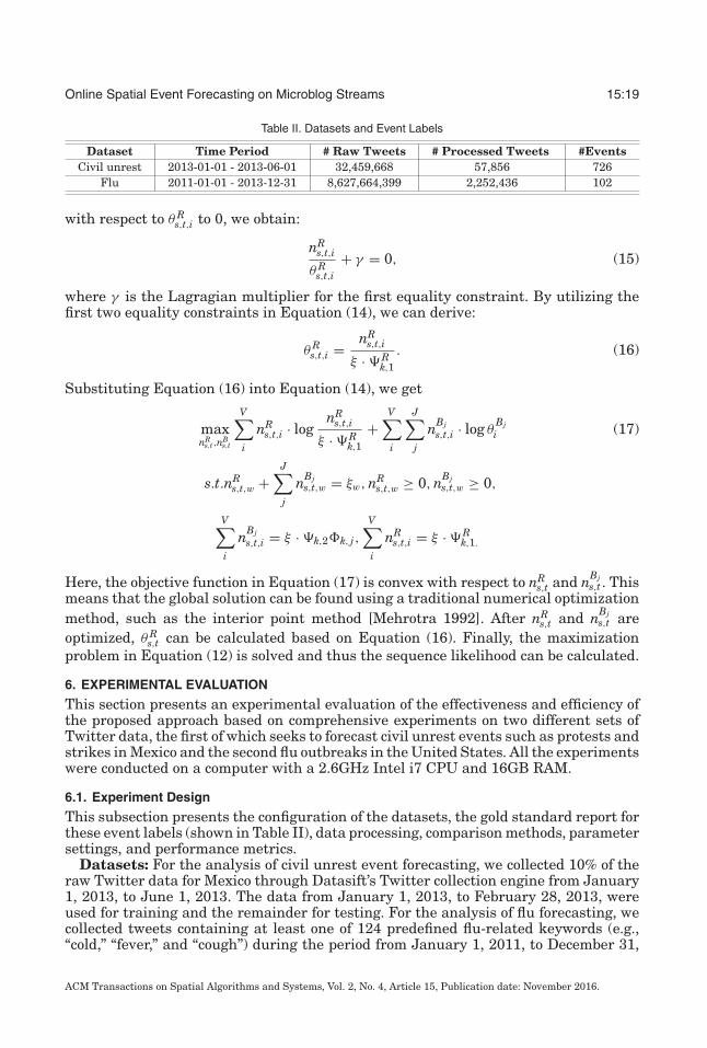
Table II. Datasets and Event Labels
Dataset Time Period # Raw Tweets # Processed Tweets #EventsCivil unrest 2013-01-01 - 2013-06-01 32,459,668 57,856 726
Flu 2011-01-01 - 2013-12-31 8,627,664,399 2,252,436 102
with respect to θ Rs,t,i to 0, we obtain:
nRs,t,i
θ Rs,t,i
+ γ = 0, (15)
where γ is the Lagragian multiplier for the first equality constraint. By utilizing thefirst two equality constraints in Equation (14), we can derive:
θ Rs,t,i = nR
s,t,i
ξ · �Rk,1
. (16)
Substituting Equation (16) into Equation (14), we get
maxnR
s,t,nBs,t
V∑i
nRs,t,i · log
nRs,t,i
ξ · �Rk,1
+V∑i
J∑j
nBjs,t,i · log θ
Bji (17)
s.t.nRs,t,w +
J∑j
nBjs,t,w = ξw, nR
s,t,w ≥ 0, nBjs,t,w ≥ 0,
V∑i
nBjs,t,i = ξ · �k,2�k, j,
V∑i
nRs,t,i = ξ · �R
k,1.
Here, the objective function in Equation (17) is convex with respect to nRs,t and nBj
s,t . Thismeans that the global solution can be found using a traditional numerical optimizationmethod, such as the interior point method [Mehrotra 1992]. After nR
s,t and nBjs,t are
optimized, θ Rs,t can be calculated based on Equation (16). Finally, the maximization
problem in Equation (12) is solved and thus the sequence likelihood can be calculated.
6. EXPERIMENTAL EVALUATION
This section presents an experimental evaluation of the effectiveness and efficiency ofthe proposed approach based on comprehensive experiments on two different sets ofTwitter data, the first of which seeks to forecast civil unrest events such as protests andstrikes in Mexico and the second flu outbreaks in the United States. All the experimentswere conducted on a computer with a 2.6GHz Intel i7 CPU and 16GB RAM.
6.1. Experiment Design
This subsection presents the configuration of the datasets, the gold standard report forthese event labels (shown in Table II), data processing, comparison methods, parametersettings, and performance metrics.
Datasets: For the analysis of civil unrest event forecasting, we collected 10% of theraw Twitter data for Mexico through Datasift’s Twitter collection engine from January1, 2013, to June 1, 2013. The data from January 1, 2013, to February 28, 2013, wereused for training and the remainder for testing. For the analysis of flu forecasting, wecollected tweets containing at least one of 124 predefined flu-related keywords (e.g.,“cold,” “fever,” and “cough”) during the period from January 1, 2011, to December 31,
ACM Transactions on Spatial Algorithms and Systems, Vol. 2, No. 4, Article 15, Publication date: November 2016.
15:20 L. Zhao et al.
2013, from across the United States. The data from January 1, 2011, to January 1,2013, were used for training and the subsequent tweets for testing.
Gold Standard Report of Event Labels: The civil unrest forecasting results werevalidated against a labeled set known as the Gold Standard Report (GSR) that wasexclusively provided by MITRE (see Ramakrishnan et al. [2014] for more details). TheGSR was organized by manually harvesting civil unrest event reports from the 10most significant news outlets2 in Mexico and the world, as ranked by InternationalMedia and Newspapers3 There were a total of 726 events during the period January1, 2013, to Junr 1, 2013. An example of a labeled GSR event is given by the tuple:(CITY = “Hermosillo”, STATE = “Sonora”, COUNTRY = “Mexico”, DATE = “2013-01-20”). The forecasting results for the flu outbreaks were validated against the flustatistics reported by the Centers for Disease Control and Prevention (CDC). CDCpublishes the weekly influenza-like illness (ILI) activity level within each state in theUnited States using the proportion of the outpatient visits to healthcare providers forILI. There are four ILI activity levels: minimal, low, moderate, and high, where thelevel “high” corresponds to a salient flu outbreak and is thus considered for forecasting.There were a total of 102 events during the period January 1, 2011, to December 31,2013. An example of a CDC flu outbreak event i: (STATE = “Michigan”, COUNTRY =“United States”, WEEK = “01-06-2013 to 01-12-2013”).
Data Preprocessing: For the first dataset, three labelers collectively labeled 20,906tweets in both English and Spanish during June 2012 to February 2013. After two hadlabeled all the tweets into positive (i.e., relevant to civil unrest) or negative, all thetweets where they disagreed were sent to the third labeler for final determination.Consequently, the tweets were categorized as 6,793 positive and 14,113 negative, andthe results used to train a linear SVM classifier. For the second dataset, we utilized thelabeled set in Lamb et al. [2013] and used these to train a linear SVM to identify tweetsrelevant to the flu. Both SVMs were generated based on unigram features containingall the distinct words with frequencies greater than 20 in the individual datasets.The trained SVM classifiers extracted the tweets deemed relevant to civil unrest andflu from the respective datasets. The locations of the tweets were extracted from thegeotags (coordinates and places); those tweets without geotags were discarded.
Comparison Methods: There are four proposed approaches evaluated in this arti-cle: STM-I, STM-S, and their two online versions, namely STM-I (online) and STM-S(online). Our proposed approaches were compared with four representative methodsand one baseline method. The Autoregressive Exogenous Model (ARX) [Achrekar et al.2011] assumes that for each separate location, the count of future events is dependenton both the count of historical events and the tweet volume. In forecasting, an out-put above “1” indicates that an event has occurred; otherwise, no event is deemed tohave occurred. The Linear Regression (LinReg) model [Arias et al. 2013; Bollen et al.2011; He et al. 2013; O’Connor et al. 2010] assumes that for each separate locationthere is a linear relationship between tweet observations and event occurrences (“0”denotes nonoccurrence, “1” denotes occurrence). The input feature here is the volumeof domain-related tweets. When forecasting, an output below 0.5 indicates no event;an output over 0.5 indicates that an event has occurred. In the Logistic Regression(LogReg) model [Wang et al. 2012b], event forecasting is treated as a classificationproblem. Here, the input features are the proportions of latent topics extracted fromthe tweet texts coming from a specific location based on the latent dirichlet alloca-tion. The output is 0 if there is no event and 1, if there is one. The Kernel DensityEstimation-Based Logistic Regression (KDE LogReg) model [Gerber 2014] forecasts
2These are La Jornada, Reforma, Milenio, The New York Times, The Guardian, The Wall Street Journal,The Washington Post, The International Herald Tribune, The Times of London, and Infolatam.3International Media and Newspapers website. Available: http://www.4imn.com/. Accessed on Oct 1, 2014.
ACM Transactions on Spatial Algorithms and Systems, Vol. 2, No. 4, Article 15, Publication date: November 2016.
Online Spatial Event Forecasting on Microblog Streams 15:21
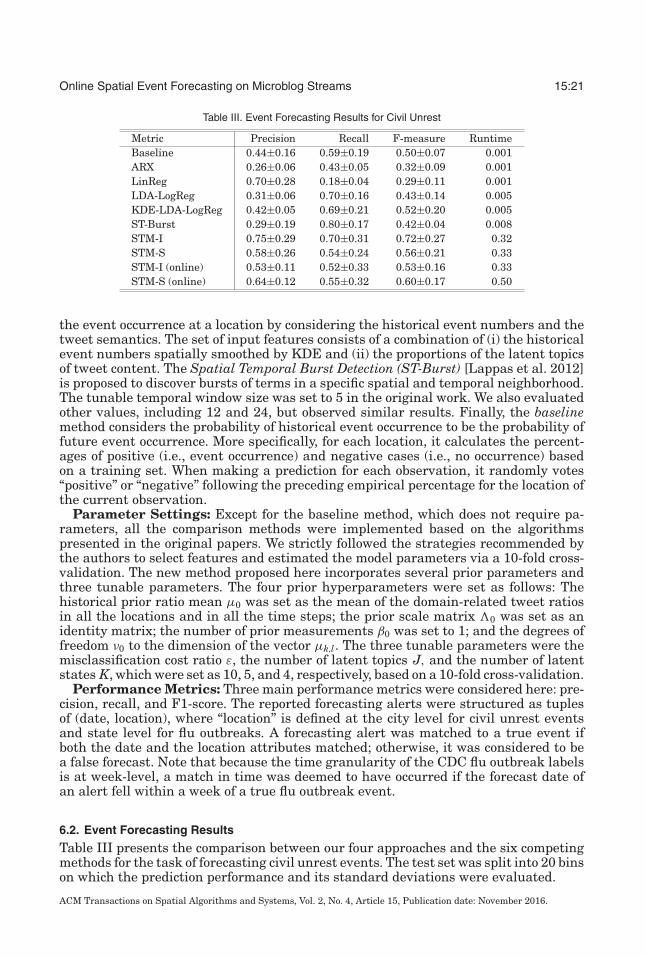
Table III. Event Forecasting Results for Civil Unrest
Metric Precision Recall F-measure RuntimeBaseline 0.44±0.16 0.59±0.19 0.50±0.07 0.001ARX 0.26±0.06 0.43±0.05 0.32±0.09 0.001LinReg 0.70±0.28 0.18±0.04 0.29±0.11 0.001LDA-LogReg 0.31±0.06 0.70±0.16 0.43±0.14 0.005KDE-LDA-LogReg 0.42±0.05 0.69±0.21 0.52±0.20 0.005ST-Burst 0.29±0.19 0.80±0.17 0.42±0.04 0.008STM-I 0.75±0.29 0.70±0.31 0.72±0.27 0.32STM-S 0.58±0.26 0.54±0.24 0.56±0.21 0.33STM-I (online) 0.53±0.11 0.52±0.33 0.53±0.16 0.33STM-S (online) 0.64±0.12 0.55±0.32 0.60±0.17 0.50
the event occurrence at a location by considering the historical event numbers and thetweet semantics. The set of input features consists of a combination of (i) the historicalevent numbers spatially smoothed by KDE and (ii) the proportions of the latent topicsof tweet content. The Spatial Temporal Burst Detection (ST-Burst) [Lappas et al. 2012]is proposed to discover bursts of terms in a specific spatial and temporal neighborhood.The tunable temporal window size was set to 5 in the original work. We also evaluatedother values, including 12 and 24, but observed similar results. Finally, the baselinemethod considers the probability of historical event occurrence to be the probability offuture event occurrence. More specifically, for each location, it calculates the percent-ages of positive (i.e., event occurrence) and negative cases (i.e., no occurrence) basedon a training set. When making a prediction for each observation, it randomly votes“positive” or “negative” following the preceding empirical percentage for the location ofthe current observation.
Parameter Settings: Except for the baseline method, which does not require pa-rameters, all the comparison methods were implemented based on the algorithmspresented in the original papers. We strictly followed the strategies recommended bythe authors to select features and estimated the model parameters via a 10-fold cross-validation. The new method proposed here incorporates several prior parameters andthree tunable parameters. The four prior hyperparameters were set as follows: Thehistorical prior ratio mean μ0 was set as the mean of the domain-related tweet ratiosin all the locations and in all the time steps; the prior scale matrix 0 was set as anidentity matrix; the number of prior measurements β0 was set to 1; and the degrees offreedom ν0 to the dimension of the vector μk,l. The three tunable parameters were themisclassification cost ratio ε, the number of latent topics J, and the number of latentstates K, which were set as 10, 5, and 4, respectively, based on a 10-fold cross-validation.
Performance Metrics: Three main performance metrics were considered here: pre-cision, recall, and F1-score. The reported forecasting alerts were structured as tuplesof (date, location), where “location” is defined at the city level for civil unrest eventsand state level for flu outbreaks. A forecasting alert was matched to a true event ifboth the date and the location attributes matched; otherwise, it was considered to bea false forecast. Note that because the time granularity of the CDC flu outbreak labelsis at week-level, a match in time was deemed to have occurred if the forecast date ofan alert fell within a week of a true flu outbreak event.
6.2. Event Forecasting Results
Table III presents the comparison between our four approaches and the six competingmethods for the task of forecasting civil unrest events. The test set was split into 20 binson which the prediction performance and its standard deviations were evaluated.
ACM Transactions on Spatial Algorithms and Systems, Vol. 2, No. 4, Article 15, Publication date: November 2016.
15:22 L. Zhao et al.
Table IV. Event Forecasting Results for the Flu Dataset
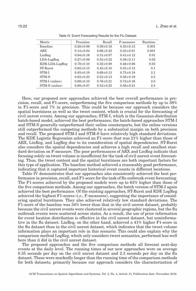
Metric Precision Recall F-measure RuntimeBaseline 0.28±0.09 0.39±0.16 0.33±0.13 0.001ARX 0.14±0.04 0.66±0.22 0.23±0.01 0.001LinReg 0.64±0.16 0.31±0.07 0.41±0.12 0.01LDA-LogReg 0.27±0.09 0.55±0.22 0.36±0.11 0.02KDE-LDA-LogReg 0.78±0.10 0.32±0.08 0.46±0.06 0.03ST-Burst 0.63±0.15 0.45±0.10 0.53±0.12 0.1STM-I 0.83±0.19 0.69±0.13 0.75±0.18 2.1STM-S 0.63±0.23 0.53±0.13 0.58±0.19 2.5STM-I (online) 0.69±0.10 0.76±0.21 0.72±0.16 2.0STM-S (online) 0.68±0.07 0.52±0.25 0.59±0.21 2.5
Here, our proposed new approaches achieved the best overall performance in pre-cision, recall, and F1-score, outperforming the five comparison methods by up to 38%in F1-score and 7% in precision. This could be because our approach considers thespatial burstiness as well as the tweet content, which is crucial for the forecasting ofcivil unrest events. Among our approaches, STM-I, which is the Gaussian-distributionbatch-based model, achieved the best performance; the batch-based approaches STM-Iand STM-S generally outperformed their online counterparts, but the online versionsstill outperformed the competing methods by a substantial margin on both precisionand recall. The proposed STM-I and STM-S have relatively high standard deviations.The KDE Logistic Regression achieved an F1-score that was 21% higher than those ofARX, LinReg, and LogReg due to its consideration of spatial dependencies. ST-Burstalso considers the spatial dependencies and achieves a high recall and smallest stan-dard deviation on F-measure. The poor performances of ARX and LinReg indicate thatfocusing solely on tweet volume is insufficient for the task of civil unrest event forecast-ing. Thus, the tweet content and the spatial burstiness are both important factors forthis type of application. The baseline method achieved a reasonably good performance,indicating that it captured important historical event counts in different locations.
Table IV demonstrates that our approaches also consistently achieved the best per-formance in precision, recall, and F1-score for the task of flu outbreak event forecasting.The F1-scores achieved by the proposed models were up to 63% higher than those ofthe five comparison methods. Among our approaches, the batch version of STM-I againachieved the best performance. Of the existing approaches, ST-Burst and KDE LogRegachieved the highest F1-scores (i.e., F-measures), suggesting the importance of consid-ering spatial burstiness. They also achieved relatively low standard deviations. TheF1-score of the baseline was 34% lower than that in the civil unrest dataset, probablybecause the civil unrest events were clustered in several geographic regions, but the fluoutbreak events were scattered across states. As a result, the use of prior informationfor event location distribution is effective in the civil unrest dataset, but noninforma-tive in the flu dataset. LinReg, on the other hand, achieved a 41% higher F1-score inthe flu dataset than in the civil unrest dataset, which indicates that the tweet volumeinformation plays an important role in this scenario. This could also explain why thecomparison method LogReg, which only considers tweet semantics, performed less wellhere than it did in the civil unrest dataset.
The proposed approaches and the five comparison methods all forecast next-dayevents at the daily level. The running times of our new approaches were on average0.35 seconds per day on the civil unrest dataset and 2.3 seconds per day on the fludataset. These were markedly longer than the running time of the comparison methodsfor both datasets, primarily because our approach considers the characterization of
ACM Transactions on Spatial Algorithms and Systems, Vol. 2, No. 4, Article 15, Publication date: November 2016.
Online Spatial Event Forecasting on Microblog Streams 15:23
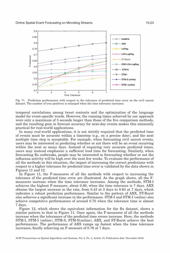
Fig. 11. Prediction performance with respect to the tolerance of predicted time error on the civil unrestdataset. The number of true positives is enlarged when the time tolerance increases.
temporal correlations among tweet contents and the optimization of the languagemodel for event-specific words. However, the running times achieved by our approachwere only a maximum of 3 seconds longer than those of the five comparison methods,and the resulting gain in forecast accuracy for next-day events makes this eminentlypractical for real-world applications.
In many real-world applications, it is not strictly required that the predicted timeof events must be accurate within a timestep (e.g., on a precise date), and the nextmultiple time step is acceptable. For example, when forecasting civil unrest events,users may be interested in predicting whether or not there will be an event occurringwithin the next so many days. Instead of requiring very accurate predicted times,users may instead emphasize a sufficient lead time for forecasting. Similarly, whenforecasting flu outbreaks, people may be interested in forecasting whether or not theinfluenza activity will be high over the next few weeks. To evaluate the performance ofall the methods in this situation, the impact of increasing the correct predictions withrespect to a higher tolerance for predicted time error is validated by the data shown inFigures 11 and 12.
In Figure 11, the F-measures of all the methods with respect to increasing thetolerance of the predicted time error are illustrated. As the graph shows, all the F-measures increase when the time tolerance increases. Among the methods, STM-Iachieves the highest F-measure, about 0.80, when the time tolerance is 7 days. ARXobtains the largest increase in the rate, from 0.43 at 2 days to 0.64 at 7 days, whichindicates a robust prediction performance. Similar to the pattern of ARX, ST-Burstalso achieves a significant increase in the performance. STM-I and STM-I (online) alsoachieve competitive performances of around 0.70 when the tolerance time is almost7 days.
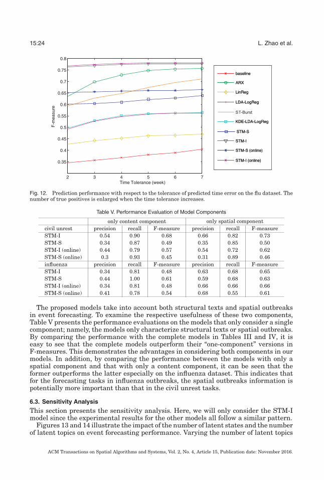
Figure 12, which shows the equivalent information for the flu dataset, shows asimilar pattern to that in Figure 11. Once again, the F-measures of all the methodsincrease when the tolerances of the predicted time errors increase. Here, the methodsSTM-I, STM-I (online), STM-S, STM-S(online), ARX, and ST-Burst achieve the bestperformances. The performance of ARX ramps up fastest when the time toleranceincreases, finally achieving an F-measure of 0.76 at 7 days.
ACM Transactions on Spatial Algorithms and Systems, Vol. 2, No. 4, Article 15, Publication date: November 2016.
15:24 L. Zhao et al.
Fig. 12. Prediction performance with respect to the tolerance of predicted time error on the flu dataset. Thenumber of true positives is enlarged when the time tolerance increases.
Table V. Performance Evaluation of Model Components
only content component only spatial componentcivil unrest precision recall F-measure precision recall F-measureSTM-I 0.54 0.90 0.68 0.66 0.82 0.73STM-S 0.34 0.87 0.49 0.35 0.85 0.50STM-I (online) 0.44 0.79 0.57 0.54 0.72 0.62STM-S (online) 0.3 0.93 0.45 0.31 0.89 0.46influenza precision recall F-measure precision recall F-measureSTM-I 0.34 0.81 0.48 0.63 0.68 0.65STM-S 0.44 1.00 0.61 0.59 0.68 0.63STM-I (online) 0.34 0.81 0.48 0.66 0.66 0.66STM-S (online) 0.41 0.78 0.54 0.68 0.55 0.61
The proposed models take into account both structural texts and spatial outbreaksin event forecasting. To examine the respective usefulness of these two components,Table V presents the performance evaluations on the models that only consider a singlecomponent; namely, the models only characterize structural texts or spatial outbreaks.By comparing the performance with the complete models in Tables III and IV, it iseasy to see that the complete models outperform their “one-component” versions inF-measures. This demonstrates the advantages in considering both components in ourmodels. In addition, by comparing the performance between the models with only aspatial component and that with only a content component, it can be seen that theformer outperforms the latter especially on the influenza dataset. This indicates thatfor the forecasting tasks in influenza outbreaks, the spatial outbreaks information ispotentially more important than that in the civil unrest tasks.
6.3. Sensitivity Analysis
This section presents the sensitivity analysis. Here, we will only consider the STM-Imodel since the experimental results for the other models all follow a similar pattern.
Figures 13 and 14 illustrate the impact of the number of latent states and the numberof latent topics on event forecasting performance. Varying the number of latent topics
ACM Transactions on Spatial Algorithms and Systems, Vol. 2, No. 4, Article 15, Publication date: November 2016.
Online Spatial Event Forecasting on Microblog Streams 15:25
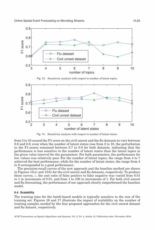
Fig. 13. Sensitivity analysis with respect to number of latent topics.
Fig. 14. Sensitivity analysis with respect to number of latent states.
from 3 to 10 caused the F1-score on the civil unrest and the flu datasets to vary between0.6 and 0.8; even when the number of latent states rose from 2 to 10, the perturbationin the F1-scores remained between 0.7 to 0.8 for both datasets, indicating that theperformance is less sensitive to the number of latent states than the latent topics inthe given value interval for the parameters. For both parameters, the performance forlow values was relatively poor. For the number of latent topics, the range from 4 to 7achieved the best performance, while for the number of latent states, the range from 4to 9 corresponded to a good performance.
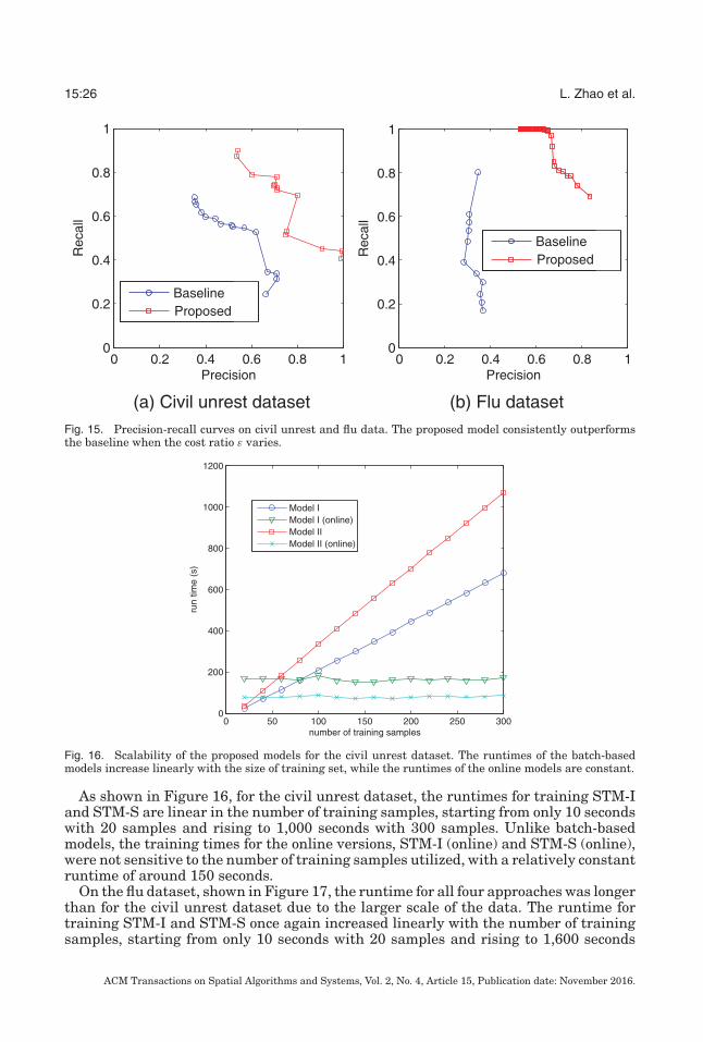
The precision-recall curves of the new approach and the baseline method are shownin Figures 15(a) and 15(b) for the civil unrest and flu datasets, respectively. To producethese curves, ε, the cost ratio of false positive to false negative was varied from 0.01to 1 in increments of 0.01, and from 1 to 100 in increments of 1. For both civil unrestand flu forecasting, the performance of our approach clearly outperformed the baselinemodel.
6.4. Scalability
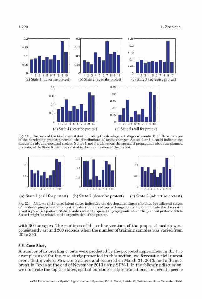
The training time for the batch-based models is typically sensitive to the size of thetraining set. Figures 16 and 17 illustrate the impact of scalability on the number oftraining samples needed by the four proposed approaches for the civil unrest datasetand flu dataset, respectively.
ACM Transactions on Spatial Algorithms and Systems, Vol. 2, No. 4, Article 15, Publication date: November 2016.
15:26 L. Zhao et al.
Fig. 15. Precision-recall curves on civil unrest and flu data. The proposed model consistently outperformsthe baseline when the cost ratio ε varies.
Fig. 16. Scalability of the proposed models for the civil unrest dataset. The runtimes of the batch-basedmodels increase linearly with the size of training set, while the runtimes of the online models are constant.
As shown in Figure 16, for the civil unrest dataset, the runtimes for training STM-Iand STM-S are linear in the number of training samples, starting from only 10 secondswith 20 samples and rising to 1,000 seconds with 300 samples. Unlike batch-basedmodels, the training times for the online versions, STM-I (online) and STM-S (online),were not sensitive to the number of training samples utilized, with a relatively constantruntime of around 150 seconds.
On the flu dataset, shown in Figure 17, the runtime for all four approaches was longerthan for the civil unrest dataset due to the larger scale of the data. The runtime fortraining STM-I and STM-S once again increased linearly with the number of trainingsamples, starting from only 10 seconds with 20 samples and rising to 1,600 seconds
ACM Transactions on Spatial Algorithms and Systems, Vol. 2, No. 4, Article 15, Publication date: November 2016.

Online Spatial Event Forecasting on Microblog Streams 15:27
Fig. 17. Scalability of the proposed models for the flu dataset. The runtimes of the batch-based modelsincrease linearly with the size of the training set, while the runtimes of the online models are constant.
Fig. 18. Illustration of all 10 topics extracted (translated into English). Topics 2 and 5 contain generalbackground words; Topics 1, 3, 4, 6, and 7 tend to include descriptive words for the protests; Topics 8 and 10focus on the words specifically calling for a protest. Topic 9 largely contains words related to disseminatinginformation on the planned protests.
ACM Transactions on Spatial Algorithms and Systems, Vol. 2, No. 4, Article 15, Publication date: November 2016.
15:28 L. Zhao et al.
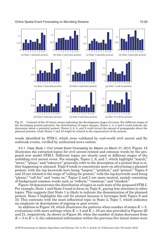
Fig. 19. Contexts of the five latent states indicating the development stages of events. For different stagesof the developing protest potential, the distributions of topics changes. States 2 and 4 could indicate thediscussion about a potential protest, States 1 and 3 could reveal the spread of propaganda about the plannedprotests, while State 5 might be related to the organization of the protest.
Fig. 20. Contexts of the three latent states indicating the development stages of events. For different stagesof the developing potential protest, the distributions of topics change. State 2 could indicate the discussionabout a potential protest, State 3 could reveal the spread of propaganda about the planned protests, whileState 1 might be related to the organization of the protest.
with 300 samples. The runtimes of the online versions of the proposed models wereconsistently around 200 seconds when the number of training samples was varied from20 to 300.
6.5. Case Study
A number of interesting events were predicted by the proposed approaches. In the twoexamples used for the case study presented in this section, we forecast a civil unrestevent that involved Mexican teachers and occurred on March 31, 2013, and a flu out-break in Texas at the end of November 2013 using STM-I. In the following discussion,we illustrate the topics, states, spatial burstiness, state transitions, and event-specific
ACM Transactions on Spatial Algorithms and Systems, Vol. 2, No. 4, Article 15, Publication date: November 2016.
Online Spatial Event Forecasting on Microblog Streams 15:29
Fig. 21. Contexts of the 10 latent states indicating the development stages of events. For different stages ofthe developing protest potential, the distributions of topics changes. States 1, 3, 4 and 5 could indicate thediscussion about a potential protest, States 2, 6, 8, and 9 could reveal the spread of propaganda about theplanned protests, while States 7 and 10 might be related to the organization of the protest.
words identified by STM-I, which were validated by real-world civil unrest and fluoutbreak events, verified by authorized news outlets.
6.5.1. Case Study I: Civil Unrest Event Forecasting for Mexico on March 31, 2013. Figure 18illustrates the extracted topics for civil unrest-related and common words by the pro-posed new model STM-I. Different topics are clearly used at different stages of theunfolding civil unrest event. For example, Topics 1, 6, and 7, which highlight “march,”“move,” “plaza,” and “takeover,” generally refer to the description of a protest that is ei-ther happening or planned. Topic 9 tends to concentrate more on advertising a plannedprotest, with the top keywords here being “largest,” “problem,” and “protest.” Topics 8and 10 are related to the stage of “calling for protest,” with the top keywords used being“please,” “call for,” and “come on.” Topics 2 and 5 are more neutral, mainly consistingof background common words such as “reflects,” “continue,” and “checked.”
Figure 19 demonstrates the distribution of topics in each state of the proposed STM-I.For example, State 1 and State 3 tend to focus on Topic 9 , paying less attention to othertopics. This suggests that State 1 is likely to indicate the dissemination of the plannedprotest. State 5 highlights the call for protest because it leverages both Topics 9 and10. This contrasts with the most influential topic in State 2, Topic 7, which indicatesan emphasis on descriptions of ongoing or past events.
In addition to Figure 19, which illustrates the patterns when number of states K = 5,evaluations with more settings when K = 3 and K = 10 are also provided in Figures 20and 21, respectively. As shown in Figure 20, when the number of states decreases fromK = 5 to K = 3, the substantial information within the previous five latent states were
ACM Transactions on Spatial Algorithms and Systems, Vol. 2, No. 4, Article 15, Publication date: November 2016.
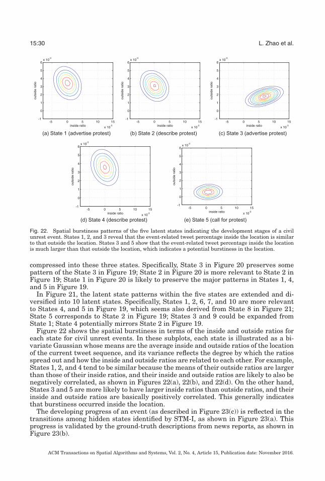
15:30 L. Zhao et al.
Fig. 22. Spatial burstiness patterns of the five latent states indicating the development stages of a civilunrest event. States 1, 2, and 3 reveal that the event-related tweet percentage inside the location is similarto that outside the location. States 3 and 5 show that the event-related tweet percentage inside the locationis much larger than that outside the location, which indicates a potential burstiness in the location.
compressed into these three states. Specifically, State 3 in Figure 20 preserves somepattern of the State 3 in Figure 19; State 2 in Figure 20 is more relevant to State 2 inFigure 19; State 1 in Figure 20 is likely to preserve the major patterns in States 1, 4,and 5 in Figure 19.
In Figure 21, the latent state patterns within the five states are extended and di-versified into 10 latent states. Specifically, States 1, 2, 6, 7, and 10 are more relevantto States 4, and 5 in Figure 19, which seems also derived from State 8 in Figure 21;State 5 corresponds to State 2 in Figure 19; States 3 and 9 could be expanded fromState 1; State 4 potentially mirrors State 2 in Figure 19.
Figure 22 shows the spatial burstiness in terms of the inside and outside ratios foreach state for civil unrest events. In these subplots, each state is illustrated as a bi-variate Gaussian whose means are the average inside and outside ratios of the locationof the current tweet sequence, and its variance reflects the degree by which the ratiosspread out and how the inside and outside ratios are related to each other. For example,States 1, 2, and 4 tend to be similar because the means of their outside ratios are largerthan those of their inside ratios, and their inside and outside ratios are likely to also benegatively correlated, as shown in Figures 22(a), 22(b), and 22(d). On the other hand,States 3 and 5 are more likely to have larger inside ratios than outside ratios, and theirinside and outside ratios are basically positively correlated. This generally indicatesthat burstiness occurred inside the location.
The developing progress of an event (as described in Figure 23(c)) is reflected in thetransitions among hidden states identified by STM-I, as shown in Figure 23(a). Thisprogress is validated by the ground-truth descriptions from news reports, as shown inFigure 23(b).
ACM Transactions on Spatial Algorithms and Systems, Vol. 2, No. 4, Article 15, Publication date: November 2016.
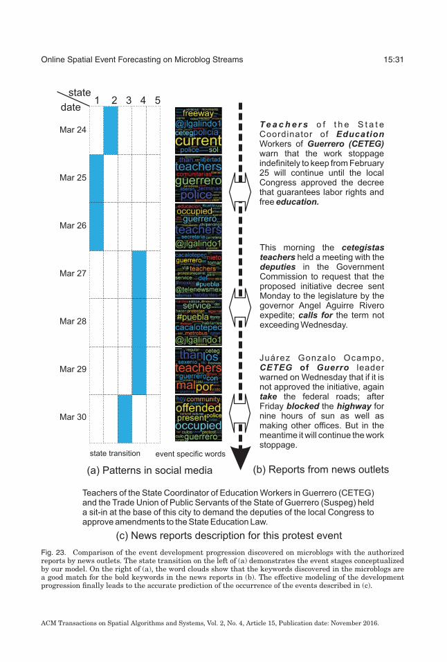
Online Spatial Event Forecasting on Microblog Streams 15:31
Fig. 23. Comparison of the event development progression discovered on microblogs with the authorizedreports by news outlets. The state transition on the left of (a) demonstrates the event stages conceptualizedby our model. On the right of (a), the word clouds show that the keywords discovered in the microblogs area good match for the bold keywords in the news reports in (b). The effective modeling of the developmentprogression finally leads to the accurate prediction of the occurrence of the events described in (c).
ACM Transactions on Spatial Algorithms and Systems, Vol. 2, No. 4, Article 15, Publication date: November 2016.
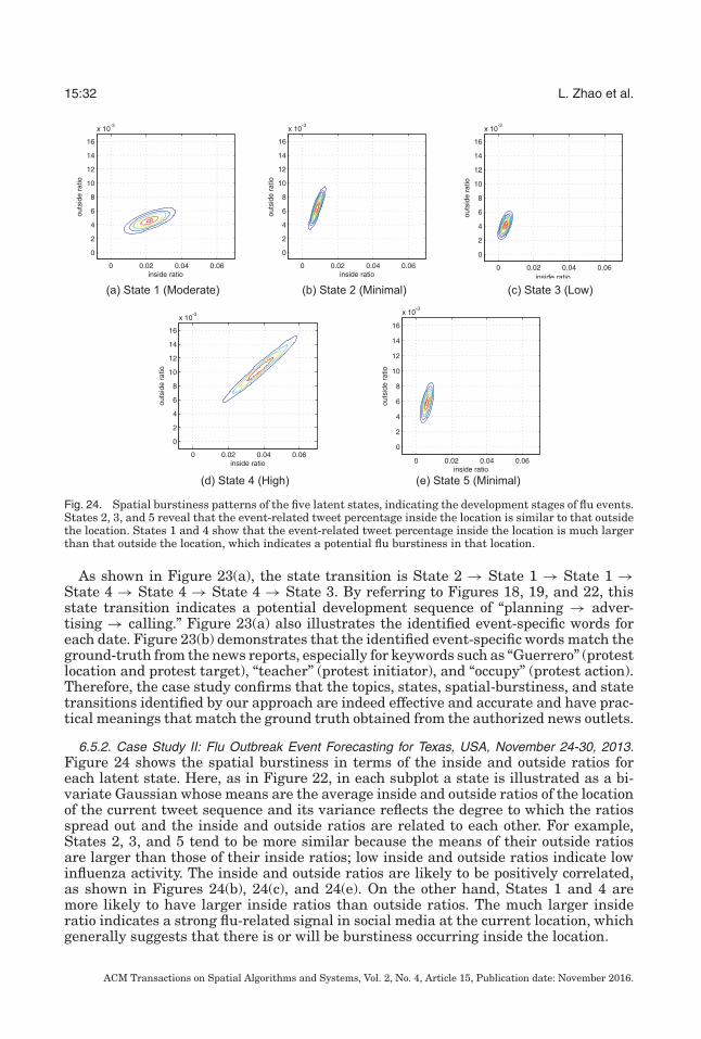
15:32 L. Zhao et al.
Fig. 24. Spatial burstiness patterns of the five latent states, indicating the development stages of flu events.States 2, 3, and 5 reveal that the event-related tweet percentage inside the location is similar to that outsidethe location. States 1 and 4 show that the event-related tweet percentage inside the location is much largerthan that outside the location, which indicates a potential flu burstiness in that location.
As shown in Figure 23(a), the state transition is State 2 → State 1 → State 1 →State 4 → State 4 → State 4 → State 3. By referring to Figures 18, 19, and 22, thisstate transition indicates a potential development sequence of “planning → adver-tising → calling.” Figure 23(a) also illustrates the identified event-specific words foreach date. Figure 23(b) demonstrates that the identified event-specific words match theground-truth from the news reports, especially for keywords such as “Guerrero” (protestlocation and protest target), “teacher” (protest initiator), and “occupy” (protest action).Therefore, the case study confirms that the topics, states, spatial-burstiness, and statetransitions identified by our approach are indeed effective and accurate and have prac-tical meanings that match the ground truth obtained from the authorized news outlets.
6.5.2. Case Study II: Flu Outbreak Event Forecasting for Texas, USA, November 24-30, 2013.Figure 24 shows the spatial burstiness in terms of the inside and outside ratios foreach latent state. Here, as in Figure 22, in each subplot a state is illustrated as a bi-variate Gaussian whose means are the average inside and outside ratios of the locationof the current tweet sequence and its variance reflects the degree to which the ratiosspread out and the inside and outside ratios are related to each other. For example,States 2, 3, and 5 tend to be more similar because the means of their outside ratiosare larger than those of their inside ratios; low inside and outside ratios indicate lowinfluenza activity. The inside and outside ratios are likely to be positively correlated,as shown in Figures 24(b), 24(c), and 24(e). On the other hand, States 1 and 4 aremore likely to have larger inside ratios than outside ratios. The much larger insideratio indicates a strong flu-related signal in social media at the current location, whichgenerally suggests that there is or will be burstiness occurring inside the location.
ACM Transactions on Spatial Algorithms and Systems, Vol. 2, No. 4, Article 15, Publication date: November 2016.
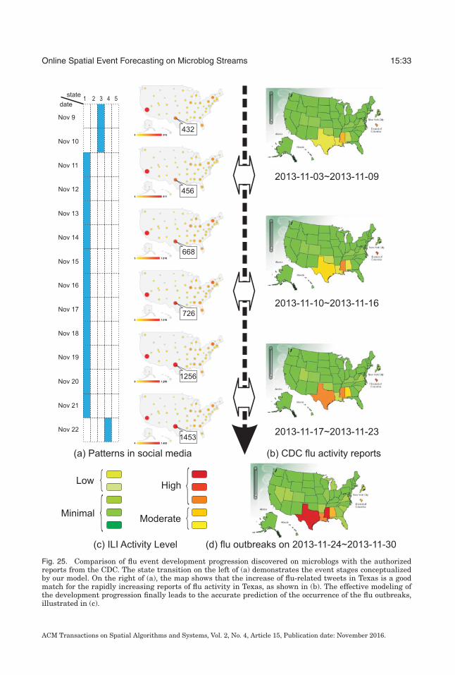
Online Spatial Event Forecasting on Microblog Streams 15:33
Fig. 25. Comparison of flu event development progression discovered on microblogs with the authorizedreports from the CDC. The state transition on the left of (a) demonstrates the event stages conceptualizedby our model. On the right of (a), the map shows that the increase of flu-related tweets in Texas is a goodmatch for the rapidly increasing reports of flu activity in Texas, as shown in (b). The effective modeling ofthe development progression finally leads to the accurate prediction of the occurrence of the flu outbreaks,illustrated in (c).
ACM Transactions on Spatial Algorithms and Systems, Vol. 2, No. 4, Article 15, Publication date: November 2016.
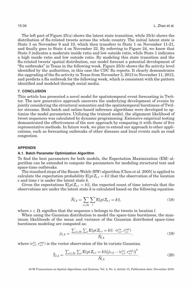
15:34 L. Zhao et al.
The left part of Figure 25(a) shows the latent state transition, while 25(b) shows thedistribution of flu-related tweets across the whole country. The initial latent state isState 3 on November 9 and 10, which then transfers to State 1 on November 11-21,and finally goes to State 4 on November 22. By referring to Figure 24, we know thatState 3 indicates a moderate inside ratio and low outside ratio, while State 1 indicatesa high inside ratio and low outside ratio. By modeling this state transition and theflu-related tweets’ spatial distribution, our model forecast a potential development of“flu outbreaks” in Texas in the following week. Figure 25(b) shows the flu activity levelidentified by the authorities, in this case the CDC flu reports. It clearly demonstratesthe upgrading of the flu activity in Texas from November 3, 2013 to November 11, 2013,and predicts a flu outbreak for the following week, which is consistent with the patternidentified and modeled through social media.
7. CONCLUSION
This article has presented a novel model for spatiotemporal event forecasting in Twit-ter. The new generative approach uncovers the underlying development of events byjointly considering the structural semantics and the spatiotemporal burstiness of Twit-ter streams. Both batch and online-based inference algorithms were developed to op-timize the model parameters. Utilizing the trained model, the alignment likelihood oftweet sequences was calculated by dynamic programming. Extensive empirical testingdemonstrated the effectiveness of the new approach by comparing it with those of fiverepresentative methods. In future work, we plan to extend our approach to other appli-cations, such as forecasting outbreaks of other diseases and local events such as roadcongestion.
APPENDIX
A.1. Batch Parameter Optimization Algorithm
To find the best parameters for both models, the Expectation Maximization (EM) al-gorithm can be extended to compute the parameters for modeling structural text andspace-time outbreaks.
The standard steps of the Baum-Welch (BW) algorithm [Chen et al. 2005] is applied tocalculate the expectation probability E[p(Zs,t = k)] that the observation of the locations and time t is under the latent state k.
Given the expectations E[p(Zs,t = k)], the expected count of time intervals that theobservations are under the latent state k is calculated based on the following equation:
Nl,k =∑s⊆Dl
∑t
E[p(Zs,t = k)], (18)
where s ∈ Dl signifies that the sequence s belongs to the tweets in location l.When using the Gaussian distribution to model the space-time burstiness, the max-
imum likelihoods of the mean and variance of the Gaussian distributed space-timeburstiness modeling are computed as:
μl,k =∑
s⊆Dl
∑t E[p(Zs,t = k)] · (rin
s,t, routs,t )
Nl,k, (19)
where (rins,t, rout
s,t ) is the vector observation of the bi-variate Gaussian.
�l,k =∑
s⊆Dl
∑t E[p(Zs,t = k)]
(μl,k − (rin
s,t, routs,t )
)2
Nl,k. (20)
ACM Transactions on Spatial Algorithms and Systems, Vol. 2, No. 4, Article 15, Publication date: November 2016.
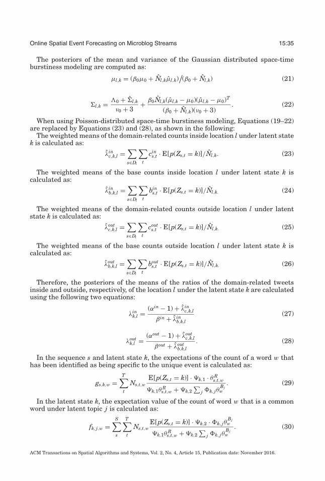
Online Spatial Event Forecasting on Microblog Streams 15:35
The posteriors of the mean and variance of the Gaussian distributed space-timeburstiness modeling are computed as:
μl,k = (β0μ0 + Nl,kμl,k)/(β0 + Nl,k) (21)
�l,k = 0 + �l,k
ν0 + 3+ β0 Nl,k(μl,k − μ0)(μl,k − μ0)T
(β0 + Nl,k)(ν0 + 3). (22)
When using Poisson-distributed space-time burstiness modeling, Equations (19–22)are replaced by Equations (23) and (28), as shown in the following:
The weighted means of the domain-related counts inside location l under latent statek is calculated as:
λinc,k,l =
∑s∈Dl
∑t
cins,t · E[p(Zs,t = k)]/Nl,k. (23)
The weighted means of the base counts inside location l under latent state k iscalculated as:
λinb,k,l =
∑s∈Dl
∑t
bins,t · E[p(Zs,t = k)]/Nl,k. (24)
The weighted means of the domain-related counts outside location l under latentstate k is calculated as:
λoutc,k,l =
∑s∈Dl
∑t
couts,t · E[p(Zs,t = k)]/Nl,k. (25)
The weighted means of the base counts outside location l under latent state k iscalculated as:
λoutb,k,l =
∑s∈Dl
∑t
bouts,t · E[p(Zs,t = k)]/Nl,k. (26)
Therefore, the posteriors of the means of the ratios of the domain-related tweetsinside and outside, respectively, of the location l under the latent state k are calculatedusing the following two equations:
λink,l = (αin − 1) + λin
c,k,l
βin + λinb,k,l
(27)
λoutk,l = (αout − 1) + λout
c,k,l
βout + λoutb,k,l
. (28)
In the sequence s and latent state k, the expectations of the count of a word w thathas been identified as being specific to the unique event is calculated as:
gs,k,w =T∑t
Ns,t,wE[p(Zs,t = k)] · �k,1 · θ R
s,t,w
�k,1θRs,t,w + �k,2
∑j �k, jθ
Bjw
. (29)
In the latent state k, the expectation value of the count of word w that is a commonword under latent topic j is calculated as:
fk, j,w =S∑s
T∑t
Ns,t,wE[p(Zs,t = k)] · �k,2 · �k, jθ
Bjw
�k,1θRs,t,w + �k,2
∑j �k, jθ
Bjw
. (30)
ACM Transactions on Spatial Algorithms and Systems, Vol. 2, No. 4, Article 15, Publication date: November 2016.
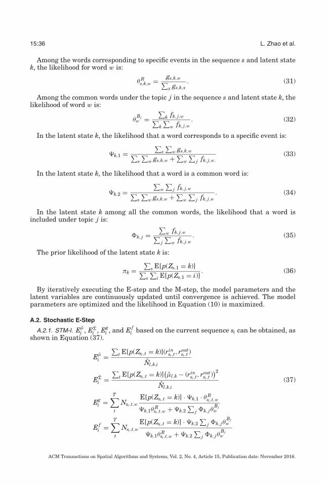
15:36 L. Zhao et al.
Among the words corresponding to specific events in the sequence s and latent statek, the likelihood for word w is:
θ Rs,k,w = gs,k,w∑
x gs,k,x. (31)
Among the common words under the topic j in the sequence s and latent state k, thelikelihood of word w is:
θBjw =
∑k fk, j,w∑
k∑
w fk, j,w. (32)
In the latent state k, the likelihood that a word corresponds to a specific event is:
�k,1 =∑
s∑
w gs,k,w∑s∑
w gs,k,w + ∑w
∑j fk, j,w.
(33)
In the latent state k, the likelihood that a word is a common word is:
�k,2 =∑
w
∑j fk, j,w∑
s∑
w gs,k,w + ∑w
∑j fk, j,w
. (34)
In the latent state k among all the common words, the likelihood that a word isincluded under topic j is:
�k, j =∑
w fk, j,w∑j∑
w fk, j,w. (35)
The prior likelihood of the latent state k is:
πk =∑
s E[p(Zs,1 = k)]∑s∑
i E[p(Zs,1 = i)]. (36)
By iteratively executing the E-step and the M-step, the model parameters and thelatent variables are continuously updated until convergence is achieved. The modelparameters are optimized and the likelihood in Equation (10) is maximized.
A.2. Stochastic E-Step
A.2.1. STM-I. Eμ
i , E�i , Eg
i , and E fi based on the current sequence si can be obtained, as
shown in Equation (37).
Eμ
i =∑
t E[p(Zsi ,t = k)](rinsi ,t, rout
si ,t )
Nl,k,i
E�i =
∑t E[p(Zsi ,t = k)]
(μl,k − (rin
si ,t, routsi ,t )
)2
Nl,k,i(37)
Egi =
T∑t
Nsi ,t,wE[p(Zsi ,t = k)] · �k,1 · θ R
si ,t,w
�k,1θRsi ,t,w + �k,2
∑j �k, jθ
Bjw
E fi =
T∑t
Nsi ,t,wE[p(Zsi ,t = k)] · �k,2
∑j �k, jθ
Bjw
�k,1θRsi ,t,w + �k,2
∑j �k, jθ
Bjw
ACM Transactions on Spatial Algorithms and Systems, Vol. 2, No. 4, Article 15, Publication date: November 2016.
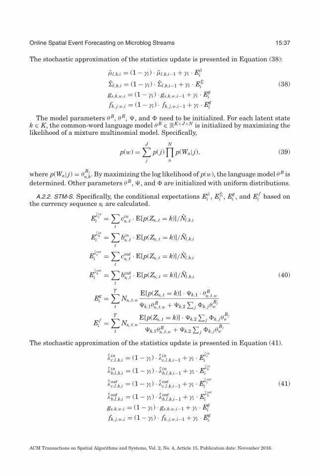
Online Spatial Event Forecasting on Microblog Streams 15:37
The stochastic approximation of the statistics update is presented in Equation (38):
μl,k,i = (1 − γi) · μl,k,i−1 + γi · Eμ
i
�l,k,i = (1 − γi) · �l,k,i−1 + γi · E�i (38)
gs,k,w,i = (1 − γi) · gs,k,w,i−1 + γi · Egi
fk, j,w,i = (1 − γi) · fk, j,w,i−1 + γi · Egi
The model parameters θ B, θ R, �, and � need to be initialized. For each latent statek ∈ K, the common-word language model θ B ∈ R
K×J×N is initialized by maximizing thelikelihood of a mixture multinomial model. Specifically,
p(w) =J∑j
p( j)N∏n
p(Wn| j), (39)
where p(Wn| j) = θBjn,k. By maximizing the log likelihood of p(w), the language model θ B is
determined. Other parameters θ R, �, and � are initialized with uniform distributions.
A.2.2. STM-S. Specifically, the conditional expectations Eμ
i , E�i , Eg
i , and E fi based on
the currency sequence si are calculated.
Eλinc
i =∑
t
cinsi ,t · E[p(Zsi ,t = k)]/Nl,k,i
Eλinb
i =∑
t
binsi ,t · E[p(Zsi ,t = k)]/Nl,k,i
Eλoutc
i =∑
t
coutsi ,t · E[p(Zsi ,t = k)]/Nl,k,i
Eλoutb
i =∑
t
boutsi ,t · E[p(Zsi ,t = k)]/Nl,k,i (40)
Egi =
T∑t
Nsi ,t,wE[p(Zsi ,t = k)] · �k,1 · θ R
si ,t,w
�k,1θRsi ,t,w + �k,2
∑j �k, jθ
Bjw
E fi =
T∑t
Nsi ,t,wE[p(Zsi ,t = k)] · �k,2
∑j �k, jθ
Bjw
�k,1θRsi ,t,w + �k,2
∑j �k, jθ
Bjw
The stochastic approximation of the statistics update is presented in Equation (41).
λinc,l,k,i = (1 − γi) · λin
c,l,k,i−1 + γi · Eλinc
i
λinb,l,k,i = (1 − γi) · λin
b,l,k,i−1 + γi · Eλinb
i
λoutc,l,k,i = (1 − γi) · λout
c,l,k,i−1 + γi · Eλoutc
i (41)
λoutb,l,k,i = (1 − γi) · λout
b,l,k,i−1 + γi · Eλoutb
i
gs,k,w,i = (1 − γi) · gs,k,w,i−1 + γi · Egi
fk, j,w,i = (1 − γi) · fk, j,w,i−1 + γi · Egi
ACM Transactions on Spatial Algorithms and Systems, Vol. 2, No. 4, Article 15, Publication date: November 2016.
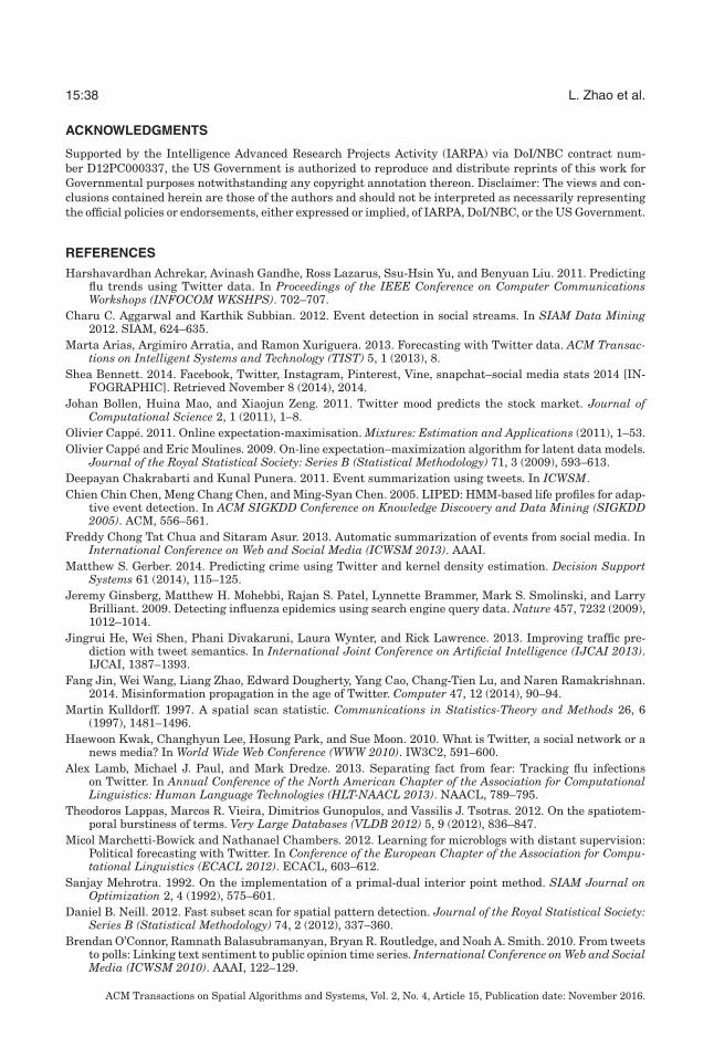
15:38 L. Zhao et al.
ACKNOWLEDGMENTS
Supported by the Intelligence Advanced Research Projects Activity (IARPA) via DoI/NBC contract num-ber D12PC000337, the US Government is authorized to reproduce and distribute reprints of this work forGovernmental purposes notwithstanding any copyright annotation thereon. Disclaimer: The views and con-clusions contained herein are those of the authors and should not be interpreted as necessarily representingthe official policies or endorsements, either expressed or implied, of IARPA, DoI/NBC, or the US Government.
REFERENCES
Harshavardhan Achrekar, Avinash Gandhe, Ross Lazarus, Ssu-Hsin Yu, and Benyuan Liu. 2011. Predictingflu trends using Twitter data. In Proceedings of the IEEE Conference on Computer CommunicationsWorkshops (INFOCOM WKSHPS). 702–707.
Charu C. Aggarwal and Karthik Subbian. 2012. Event detection in social streams. In SIAM Data Mining2012. SIAM, 624–635.
Marta Arias, Argimiro Arratia, and Ramon Xuriguera. 2013. Forecasting with Twitter data. ACM Transac-tions on Intelligent Systems and Technology (TIST) 5, 1 (2013), 8.
Shea Bennett. 2014. Facebook, Twitter, Instagram, Pinterest, Vine, snapchat–social media stats 2014 [IN-FOGRAPHIC]. Retrieved November 8 (2014), 2014.
Johan Bollen, Huina Mao, and Xiaojun Zeng. 2011. Twitter mood predicts the stock market. Journal ofComputational Science 2, 1 (2011), 1–8.
Olivier Cappe. 2011. Online expectation-maximisation. Mixtures: Estimation and Applications (2011), 1–53.Olivier Cappe and Eric Moulines. 2009. On-line expectation–maximization algorithm for latent data models.
Journal of the Royal Statistical Society: Series B (Statistical Methodology) 71, 3 (2009), 593–613.Deepayan Chakrabarti and Kunal Punera. 2011. Event summarization using tweets. In ICWSM.Chien Chin Chen, Meng Chang Chen, and Ming-Syan Chen. 2005. LIPED: HMM-based life profiles for adap-
tive event detection. In ACM SIGKDD Conference on Knowledge Discovery and Data Mining (SIGKDD2005). ACM, 556–561.
Freddy Chong Tat Chua and Sitaram Asur. 2013. Automatic summarization of events from social media. InInternational Conference on Web and Social Media (ICWSM 2013). AAAI.
Matthew S. Gerber. 2014. Predicting crime using Twitter and kernel density estimation. Decision SupportSystems 61 (2014), 115–125.
Jeremy Ginsberg, Matthew H. Mohebbi, Rajan S. Patel, Lynnette Brammer, Mark S. Smolinski, and LarryBrilliant. 2009. Detecting influenza epidemics using search engine query data. Nature 457, 7232 (2009),1012–1014.
Jingrui He, Wei Shen, Phani Divakaruni, Laura Wynter, and Rick Lawrence. 2013. Improving traffic pre-diction with tweet semantics. In International Joint Conference on Artificial Intelligence (IJCAI 2013).IJCAI, 1387–1393.
Fang Jin, Wei Wang, Liang Zhao, Edward Dougherty, Yang Cao, Chang-Tien Lu, and Naren Ramakrishnan.2014. Misinformation propagation in the age of Twitter. Computer 47, 12 (2014), 90–94.
Martin Kulldorff. 1997. A spatial scan statistic. Communications in Statistics-Theory and Methods 26, 6(1997), 1481–1496.
Haewoon Kwak, Changhyun Lee, Hosung Park, and Sue Moon. 2010. What is Twitter, a social network or anews media? In World Wide Web Conference (WWW 2010). IW3C2, 591–600.
Alex Lamb, Michael J. Paul, and Mark Dredze. 2013. Separating fact from fear: Tracking flu infectionson Twitter. In Annual Conference of the North American Chapter of the Association for ComputationalLinguistics: Human Language Technologies (HLT-NAACL 2013). NAACL, 789–795.
Theodoros Lappas, Marcos R. Vieira, Dimitrios Gunopulos, and Vassilis J. Tsotras. 2012. On the spatiotem-poral burstiness of terms. Very Large Databases (VLDB 2012) 5, 9 (2012), 836–847.
Micol Marchetti-Bowick and Nathanael Chambers. 2012. Learning for microblogs with distant supervision:Political forecasting with Twitter. In Conference of the European Chapter of the Association for Compu-tational Linguistics (ECACL 2012). ECACL, 603–612.
Sanjay Mehrotra. 1992. On the implementation of a primal-dual interior point method. SIAM Journal onOptimization 2, 4 (1992), 575–601.
Daniel B. Neill. 2012. Fast subset scan for spatial pattern detection. Journal of the Royal Statistical Society:Series B (Statistical Methodology) 74, 2 (2012), 337–360.
Brendan O’Connor, Ramnath Balasubramanyan, Bryan R. Routledge, and Noah A. Smith. 2010. From tweetsto polls: Linking text sentiment to public opinion time series. International Conference on Web and SocialMedia (ICWSM 2010). AAAI, 122–129.
ACM Transactions on Spatial Algorithms and Systems, Vol. 2, No. 4, Article 15, Publication date: November 2016.
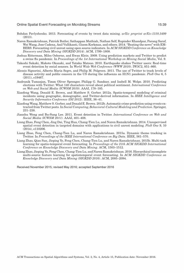
Online Spatial Event Forecasting on Microblog Streams 15:39
Bohdan Pavlyshenko. 2013. Forecasting of events by tweet data mining. arXiv preprint arXiv:1310.3499(2013).
Naren Ramakrishnan, Patrick Butler, Sathappan Muthiah, Nathan Self, Rupinder Khandpur, Parang Saraf,Wei Wang, Jose Cadena, Anil Vullikanti, Gizem Korkmaz, and others. 2014. “Beating the news” with EM-BERS: Forecasting civil unrest using open source indicators. In ACM SIGKDD Conference on KnowledgeDiscovery and Data Mining (SIGKDD 2014). ACM, 1799–1808.
Joshua Ritterman, Miles Osborne, and Ewan Klein. 2009. Using prediction markets and Twitter to predicta swine flu pandemic. In Proceedings of the 1st International Workshop on Mining Social Media, Vol. 9.
Takeshi Sakaki, Makoto Okazaki, and Yutaka Matsuo. 2010. Earthquake shakes Twitter users: Real-timeevent detection by social sensors. In World Wide Web Conference (WWW 2010). IW3C2, 851–860.
Alessio Signorini, Alberto Maria Segre, and Philip M. Polgreen. 2011. The use of Twitter to track levels ofdisease activity and public concern in the US during the influenza an H1N1 pandemic. PloS One 6, 5(2011), e19467.
Andranik Tumasjan, Timm Oliver Sprenger, Philipp G. Sandner, and Isabell M. Welpe. 2010. Predictingelections with Twitter: What 140 characters reveal about political sentiment. International Conferenceon Web and Social Media (ICWSM 2010). AAAI, 178–185.
Xiaofeng Wang, Donald E. Brown, and Matthew S. Gerber. 2012a. Spatio-temporal modeling of criminalincidents using geographic, demographic, and Twitter-derived information. In IEEE Intelligence andSecurity Informatics Conference (ISI 2012). IEEE, 36–41.
Xiaofeng Wang, Matthew S. Gerber, and Donald E. Brown. 2012b. Automatic crime prediction using events ex-tracted from Twitter posts. In Social Computing, Behavioral-Cultural Modeling and Prediction. Springer,231–238.
Jianshu Weng and Bu-Sung Lee. 2011. Event detection in Twitter. International Conference on Web andSocial Media (ICWSM 2011). AAAI, 401–408.
Liang Zhao, Feng Chen, Jing Dai, Ting Hua, Chang-Tien Lu, and Naren Ramakrishnan. 2014. Unsupervisedspatial event detection in targeted domains with applications to civil unrest modeling. PloS One 9, 10(2014), e110206.
Liang Zhao, Feng Chen, Chang-Tien Lu, and Naren Ramakrishnan. 2015a. Dynamic theme tracking inTwitter. In Proceedings of the IEEE International Conference on Big Data. IEEE, 561–570.
Liang Zhao, Qian Sun, Jieping Ye, Feng Chen, Chang-Tien Lu, and Naren Ramakrishnan. 2015b. Multi-tasklearning for spatio-temporal event forecasting. In Proceedings of the 21th ACM SIGKDD InternationalConference on Knowledge Discovery and Data Mining. ACM, 1503–1512.
Liang Zhao, Jieping Ye, Feng Chen, Chang-Tien Lu, and Naren Ramakrishnan. 2016. Hierarchical incompletemulti-source feature learning for spatiotemporal event forecasting. In ACM SIGKDD Conference onKnowledge Discovery and Data Mining (SIGKDD 2016). ACM, 2085–2094.
Received November 2015; revised May 2016; accepted September 2016
ACM Transactions on Spatial Algorithms and Systems, Vol. 2, No. 4, Article 15, Publication date: November 2016.