spatial network based model forecasting transmission and ...may 06, 2020 · spatial network based...

Spatial Network based model forecasting transmission and control of COVID-19

Natasha Sharma,1, 2 Atul Kumar Verma,1 and Arvind Kumar Gupta1, ∗

1Department of Mathematics, Indian Institute of Technology Ropar, Rupnagar-140001, Punjab, India2PG Department of Mathematics, Kanya Maha Vidyalaya, Jalandhar-144004, Punjab, India.

The SARS-CoV-2 driven infectious novel coronavirus disease (COVID-19) has been declared apandemic by virtue of its brutal impact on the world in terms of loss on human life, health, eco-nomy, and other crucial resources. With the aim to explore more about its aspects, we adoptedthe SEIQRD (Susceptible-Exposed-Infected-Quarantine-Recovered-Death) pandemic spread witha time delay on the heterogeneous population and geography in this work. Focusing on the spatialheterogeneity, the entire population of interest in a region is divided into small distinct geograph-ical sub regions, which interact by means of migration networks across boundaries. Utilizing theestimations of the time delay differential equations based model, we analyzed the spread dynamicsof disease in a region and its sub regions. The model based numerical outcomes are validated fromreal time available data for India. We computed the approximate peak infection in forward timeand relative timespan when disease outspread halts. To further evaluate the influence of the delayon the long term system dynamics, the sensitivity analysis is performed on time delay. The mostcrucial parameter, basic reproduction number R0 and its time-dependent generalization, has beenestimated at both regional and sub regional levels. The impact of the most significant lockdownmeasure that has been implemented in India to contain the pandemic spread has been extensivelystudied by considering no lockdown scenario. A suggestion based on outcomes, for a bit relaxedlockdown, followed by an extended period of strict social distancing as one of the most effectivecontrol measures to manage COVID-19 spread is provided for India.

I. INTRODUCTION

The novel coronavirus disease, officially known as 2019-nCoV, or SARS-CoV-2 (severe acute respiratory syn-drome coronavirus 2), commonly called COVID-19, hasprovided the world with an unparallel challenge. Thefirst reported case in the COVID-19 outbreak appearedin the Wuhan city of China in December 2019, and sincethen, it has rapidly spread in 210 countries and territor-ies around the world [1]. As of April 30, 2020, a totalof 3,275,475 confirmed cases of the coronavirus and atoll of 231,576 deaths has been reported globally [2].At this moment of time, there is no definite vaccineor treatment for COVID-19. It has thrown an unpre-dictable burden on healthcare systems in the majorityof the developed as well as developing countries. Withits breakneck spread all across, World Health Organiza-tion(WHO) has declared it as a pandemic and to containthe upsurge by breaking its person to person transmis-sion chain involving significant human migration, majorsteps including partial or complete lockdowns, interna-tional travel bans, and social distancing has been widelyadopted.

In India, the first case of coronavirus pandemic wasidentified on January 30, 2020, originating from China.Since this appearance, there has been a continuous rise inthe number of infections with the total number of 33,610cases on April 30, 2020, of which there are 8,373 recover-ies and 1,075 deaths [3]. As a preventive measure, Indiaalso implemented a strict lockdown along with curfewin certain states, limiting movement of the entire pop-

∗ [email protected]

ulation to minimize social contacts. The efficiency ofsuch measures is geographically sensitive due to differentpopulation densities, social contact networks, and healthcare facilities. Though these measures are important forcontrolling the virus, they have an extensive burden onthe global economy as well. Quantitative projection ofthe effect of these measures in reducing infection is cru-cial in outlining social and economic policies. Further,understanding the transmission dynamics of COVID-19not only provides deep insights into the epidemiologicalsituation to enhance public-health planning, but such in-vestigations can also aid in the layout of alternative out-break control measures.

Knowledge of the early spread dynamics of the in-fection and figuring out the capability and performanceof applied control measures is critical for assessing theextensive outspread to occur in new regions. Besidesmedical and biological research, understanding the ur-gency to develop a predictable mathematical model forthe COVID-19 outbreak, few mathematical studies basedon statistical reasoning and simulations have been takenup in past months [4–6]. Later, accepting the challengesto explore the efficiency of various control measures sincethe outbreak, fewer studies adopted more appropriate dy-namical equations based on mathematical modeling tech-niques. Compartment models such as SI, SIR, SEIRwhich exhibits the change in the category of populationamong the susceptible (S), exposed (E), infected (I) andrecovered (R) classes have been developed and studiedto understand the spread pattern of COVID-19 in manycountries [7–11].

Further, as reported, COVID-19 has a lat-ent/incubation period (time from exposure to thedevelopment of symptoms), which is estimated to be

All rights reserved. No reuse allowed without permission. (which was not certified by peer review) is the author/funder, who has granted medRxiv a license to display the preprint in perpetuity.

The copyright holder for this preprintthis version posted May 8, 2020. ; https://doi.org/10.1101/2020.05.06.20092858doi: medRxiv preprint

NOTE: This preprint reports new research that has not been certified by peer review and should not be used to guide clinical practice.

mailto:[email protected]

https://doi.org/10.1101/2020.05.06.20092858

2

28

32

17

2

1

3

4

5

6

7

10

11

12

13

23

27

24

25

3126 22

20

21

15

14 16

18

19

9

8

30

29

E

I

R

S Q

D

Interacted

Latent Period

(no symptoms)

(a) (b)

Figure 1: (a) The map of India along with different states (represented by filled dots, numbered from 1 to 32∗). Thesolid lines shows the connections of a state with its neighboring states resulting in inter state movements. The states

with more/less than 2000 cases as on April 30, 2020 are shown by red/orange color. COVID-19 free states arerepresented by green color.The complete dataset reflecting state wise population distribution is provided in Appendix(C) in Table II. ∗Note that in the study we have not considered a few Indian states and Union Territories includingLakshadweep, Dadra and Nagar Haveli, Daman and Diu, Andaman and Nicobar Islands and Puducherry on accountof their comparatively low population density. (b) Within a state, Schematic of SEIQRD Model with time delay.

between 2 and 14 days [12]. This incubation period isvery significant as it allows the health authorities tointroduce more adequate systems for separating peoplesuspected of carrying the virus, as a way of controllingand preventing the spread of the pandemic [13]. Theinclusion of the latent period in compartment modelsgives rise to COVID-19 time delay models in which thedynamic behavior of the disease at time t depends on thestate of the system at a time prior to the delay period[14, 15]. However, these studies assume homogeneityin a large population and ignore numerical variationsoriginating from natural births, deaths, and humanmigration networks across the regions. To the amountthat population and geographic heterogeneities playcrucial roles in the infection outbreak process, in orderto pick up the vital characteristics of the pandemic, it isadvantageous to include them in the time delay model.

Capturing the critical impact of the delay period ofCOVID-19, this study presents a mathematical modelto analyze the spread of the novel coronavirus within aheterogeneous population and geography. We proposea more realistic time delay differential equations basedSEIQRD model by incorporating quarantined (Q)- con-firmed and separated infected population as well as deathdue to infection class (D) along with the optimal valuesfor model parameters, which reasonably fit the actualinfection cases of the pandemic. Spatial and stochastic

parameters like heterogeneous population, natural births,deaths, and population migration networks within a geo-graphical state (subpopulation in a country) boundarieshave been considered. Predominantly, in the presentedmodel, considering the spatial heterogeneity, the entirepopulation of the broad geographical region of interestis divided into small sub regions- states, which inter-act by means of migrations across the state boundar-ies. Moreover, there are many inevitable questions re-lated to the spread of the pandemic. How many peopleare at risk of infection ? When will be the infection atits peak and when will it end ? Are the existing controlmeasures sufficient to control the outbreak ? With theaim to explore more about the transmission of COVID-19 dynamics and to predict its potential tendency, theCOVID-19 pandemic is estimated for forward time. Thegeneral points of interest including total infected cases,infection peak, pandemic ending time are investigated.The most vital parameter, basic reproduction numberR0 and its time-dependent generalization that decides ifan originating infectious disease can extend in a popu-lation, has been estimated at both regional and its subregional levels. Additionally, the influence of the timedelay on the long term pandemic dynamics has been ex-plored. Further, we use the model to examine the impactof the most significant lockdown measure that has beenimplemented to contain the pandemic spread.



https://doi.org/10.1101/2020.05.06.20092858

3

II. MATERIAL AND METHOD

A. Generalized SEIQRD model with time delay

To estimate the trajectories of COVID-19 transmis-sion, in the proposed approach, a vast geographic regionwith heterogeneous population distribution (country) ispartitioned into n smaller sub-regions (states). To takeinto account the effect of both inter and intrastate infec-tious population, migration for these states are explicitlyincorporated (Fig. 1(a)), using population migration ad-jacency matrix λ (with order n×n). The diagonal coeffi-cients of this matrix represent the migration rate withina state while for any of its jth row, kth element indic-ates the migration factor from the jth state to the kth

state. For any two states which share no boundaries mi-gration rate is 0. Within a given state, the transmissionis handled according to a deterministic compartmentalmodel dividing the population into six epidemiologicalclasses S(t), E(t), I(t), Q(t), R(t), D(t) describing at timet the respective proportion of the susceptible cases, ex-posed cases (infected but not capable of transmitting in-fection, in a latent period), infected cases (with the in-fection spreading capacity and not yet separated fromthose who are not infected), quarantined cases (confirmedand separated infected), recovered cases and deaths ow-ing to virus cases. Fig. 1(b) shows the movement withinthe classes in model with time delay. Since the latentperiod (τ) of the COVID-19 is as long as 2 to 14 days[1], the exposed class (E) originates because of interac-tions with the amount β within susceptible (S) and in-fected class (I). Only those members of the exposed classwho survive the latency period move to the infected classwith a rate of σ. The infected population tested positivefor COVID-19 moves to quarantine class (Q) for furthertreatment with parameter ε. After a course of quarantinetreatment, either a part of its population is dischargedwith the rate δ from the hospital (R) or encounter deathdue to underline diseases (D) with an estimate γ. Anappendix (A) provides complete details of our mathem-atical model characterized by a group of ordinary differ-ential equations depicting the outbreak at time t. Theprimary model parameters, reasonably fitting the actualinfected cases till date, are described in Table I in theappendix (C).

B. Data Source

The epidemic bulletin from the World Health Organ-ization provides us with primary data on epidemiologicalresearch. According to the reports by WHO, the incub-ation period for COVID-19, which is the time betweenexposure to the virus (becoming infected) and symptomonset, is, on average 7 days; however, it can be up to 14days [1]. The average mortality rate based on historicaldata is about 3.4% [2, 11].

To check how optimal is the fitting between the actual

16 March 25 March 6 April 18 April 30 April0

1

2

3

4x 10

4

Totalinfectedcases(I+Q) India

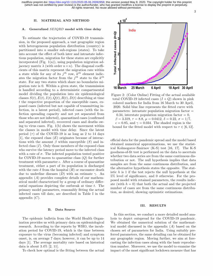
Figure 2: (Color Online) Fitting of the actual availabletotal COVID-19 infected cases (I +Q) shown in pinkcolored markers for India from 16 March to 30 April,2020. Solid blue line represents the fitted curve withparameters: intrastate population migration factor =

0.34, interstate population migration factor = 0,β = 3.319, τ = 8.8, µ = 0.0412, δ = 0.22, σ = 1/7,ε = 0.85, and γ = 0.034. The shaded region is the

bound for the fitted model with respect to τ ∈ [6, 12].

official data for the pandemic spread and the model basedobtained numerical approximations, we use the statist-ical Kolmogorov-Smirnov (K-S) test [16, 17]. The K-Sgoodness-of-fit test is performed on the data to ascertainwhether two data series are from the same continuous dis-tribution or not. The null hypothesis implies that datasamples are from the same continuous distribution, andthe alternative hypothesis states the opposite. The stat-istic h is 1 if the test rejects the null hypothesis at the5% level of significance, and 0 otherwise. For the pro-posed model with retained parameters, the results indic-ate (with h = 0) that both the actual and the projectednumber of cases are from the same continuous distribu-tion, as desired, showing optimistic estimations.

III. RESULTS

In this section, we conduct a more detailed model ana-lysis to depict outspread for the COVID-19 pandemic.We obtained the numerical solution of the mathemat-ical model discussed in the appendix (A) based on thechosen set of parameters for India. Using suitably pre-ferred parameters, the same detailing can be obtained forany geographic region. Moving further, we aim at fore-casting the infection cases along with the basic reproduc-tion number. Moreover, we use the model to examine theimpact of the most significant lockdown measure that has



https://doi.org/10.1101/2020.05.06.20092858

4

16 March 5 May 30 June 13 Aug 2 Oct0

2

4

6

7x 10

6Totalinfectedcases(I+Q)

Strict lockdown

India

(a)

16 March 12 Sept 11 March 7 Sept 14 Feb0

2

4

6

8

10

12x 10

7

Totalinfectedcases(I+Q)

No lockdown

India

(b)

1 May 25 July 18 Oct 6 Jan0

2

4

6

8

10

12x 10

4


β = 1β = 0.5

Relaxed lockdown

India

(c)

Figure 3: (Color online) Total infected cases (I +Q) with respect to time (in days) in different scenarios (a) strictlockdown (b) no lockdown (c) relaxed lockdown. In (a) blue line represents real data from 16 March to 30 April,2020. The parameters are (intrastate population migration factor, interstate population migration factor, β) =(0.34, 0, 3.319), (0.8, 0.6, 9), (0.34, 0.10, 0.5, 1) in (a-c) with common parameters τ = 8.8, µ = 0.0412, δ = 0.22,σ = 1/7, ε = 0.85, and γ = 0.034. The shaded region in (a-b) is the bound for the fitted model with respect to

τ ∈ [6, 12]. In (b) the dates 11 March, 7 Sept are for year 2021, 14 Feb for 2022; in (c) 6 Jan belong to year 2021;while remaining dates are from 2020.

16 March 5 May 24 June 13 August 2 October0

5

10

15x 10

5

Infectedcases(I)

Strict lockdown

India

(a)

16 March 13 Aug 10 Jan 16 March 6 Nov0

1

2

3

4

4.5x 10

7

Infectedcases(I)

No lockdown

India

(b)

1 May 25 July 18 Oct 6 Nov0

1

2

3

4x 10

4

Infectedcases(I)

β= 1β= 0.5

Relaxed lockdown

India

(c)

Figure 4: (Color online) Infectious cases (I) with respect to time (in days) in different cases (a) strict lockdown (b)no lockdown (c) relaxed lockdown. The parameters are (intrastate population migration factor, interstate

population migration factor, β) = (0.34, 0, 3.319), (0.8, 0.6, 9), (0.34, 0.10, 0.5, 1) in (a-c) with common parametersτ = 8.8, µ = 0.0412, δ = 0.22, σ = 1/7, ε = 0.85, and γ = 0.034. The shaded region in (a-b) is the bound for the

fitted model with respect to τ ∈ [6, 12]. In (b) the dates 10 Jan, 16 March, 6 Nov belong to year 2021 whileremaining dates are from current year 2020.

been implemented in India to contain the pandemic. Itis significant to mention that, at present, due to lack ofsufficient diagnostic test for COVID-19, the total numberof infected cases (I+Q) in any jth state, can be given by(I(t)+Q(t))αNj . Here, Nj denotes the population of thejth state, and α is considered approximately as 0.1 in therole of the current testing events [18]. Clearly, the totalinfected cases in a country with n states can be obtainedby the sum of corresponding data from the states.

At the onset, we used the proposed model to fitactual available COVID-19 infection cases for India up

to April 30, 2020 (Fig. 2). Notably, since India wentinto a strict lockdown that commenced on March 25,2020, officially published data by Ministry of Health andFamily Welfare (MoHFW), Government of India fromMarch 16, 2020 to April 30, 2020 are marked in pinkspots and are considered as a direct validation source.As expected, we can clearly see that the prediction ofthe exact number of cases diagnosed in the past time bythe model is in reasonable agreement with the real value.With an aim to estimate the potential tendency of theCOVID-19 pandemic and to examine the impact of the



https://doi.org/10.1101/2020.05.06.20092858

5

lockdown control measure we compared the infectionspread in the cases of current strict lockdown and nolockdown in place as under:

Nationwide strict Lockdown: With parametersin hand, we executed the model forward in time tovisualize the progress of the pandemic in the presentsituation of strict lockdown. Fig. 3 shows the trajectoryfor the total number of infected cases in India (Infectious+ Quarantined) in the coming months. Fig. 3(a)displays a five month forecast in the present scenarioof nationwide lockdown as a strategic move to controlthe pandemic spread. With strict lockdown measurescurrently in place, since all transport services: road,air, and rail were suspended, we set the interstatepopulation migration index to null in the populationmigration adjacency matrix λ, and the average contactsbetween susceptible and infected are considered to beproximately three. Based on these criteria, our modelfeatured a single infection peak on June 30, 2020 withthe total number of estimated infected to be around 5.2million. The outbreak is expected to be nearing its endby late August, 2020.

No Lockdown: To highlight the effectiveness ofthe ongoing national lockdown, in comparison, Fig.3(b) shows infection forecast if in case lockdown wasnot implemented. In this situation, we allowed normalmigration within the states and across the boundaries bysetting non zero estimates for diagonal and off diagonalentries in the migration adjacency matrix. However,assuming that some form of control measure wouldcontinue to be in the system to reduce social contact,we choose average contacts between susceptible andinfected to be approximately nine [18]. As anticipated,if interventions would not have been there, India mighthave experienced 18 times worst the numbers with 40million infections by mid of October, 2020 with a peakof approximately 90 million cases around April, 2021.There still would have been around 5, 00, 000 infectiouscases revealed at the end of August, 2021 as exhibitedby Fig. 4(b).

Proposed Scenario: In the third scenario, Fig.3(c) panel exhibits a rundown for a proposed protocolwith a bit relaxed lockdown, allowing restricted move-ments within and across the state boundaries beyondMay 3, 2020. This relaxation assumes gradual freedomof movement for essential activities only, thereby en-suring the upliftment of lockdown in stages to save theeconomy. Moreover, considering self awareness withinthe population, we invoked reduced average contactparameter β between susceptible and infected to beapproximately one, through social distancing impactsin this case. This alteration was required as a step tobreak or lessen human to human transmission chain ofthe virus. As likely, this consideration brings the totalnumber of infections to comparatively lower values and

5 May 24 June 13 August

0.5

1

1.5

2

2.5

3

3.5

4

Basicreproductionnumber

5 May 24 June 13 August0

5

10

15x 10

5

Infectedcases(I)

India

Figure 5: (Color Online) Basic reproduction numberwith respect to time in presence of strict lockdown for

intrastate population migration factor = 0.34, interstatepopulation migration factor = 0, β = 3.319, τ = 8.8,µ = 0.0412, δ = 0.22, σ = 1/7, ε = 0.85, and γ = 0.034.The inset figure shows infectious cases as in Fig. 4(a)

with time for same parameters.

slows the spread of the disease to manageable levels.Moreover, peak infections in the proposed scenariodecrease significantly in comparison to a strict lockdownsituation. This observation clearly highlights the factthat social distancing is one of several changes that wehave to adapt strictly in the coming weeks. To ensurethe distances are well maintained at work or publicplaces, more mature ways of monitoring, includingartificial intelligence or machine learning software, canbe used. As depicted in Fig. 3(c), as a suggestion, ifsocial distancing is enforced broadly and is maintainedin the coming months, the number of new infectionswould decrease to a significantly submissive level, andthe outbreak could eventually be controlled.

Additionally, in order to further evaluate the influenceof the delay on the long term disease dynamics, we per-formed the sensitivity analysis on τ keeping other para-meters fixed. We plotted the total infected cases andinfectious cases as a function of time for systematicallyvaried values of τ ∈ [6, 12] shown by shaded regions inFig. 2, Fig. 3 and Fig. 4. Apparently, a small changein delay has no qualitative impact on the nature of thespread, apart from shifting of the curve, thereby pre-serving the basic shape of the infection pattern. Shiftsin infection peak with varied τ provide us with a pos-sible domain window range for estimation of infectioncases owing to regional differences in India on account ofhealth, education, religion, and per capita income.

In order to capture R0 for heterogeneous populationdistribution in India, we computed its value using the



https://doi.org/10.1101/2020.05.06.20092858

6

proposed model by the relation given by Eq.(7) in theappendix (B). The estimated basic reproduction num-ber for India in the present scenario of nationwide lock-down turns out to be 1.18. Based on this value of R0, asexpected, from the transmission dynamics of the infec-tion in a strick lockdown situation, shown in Fig. 4(a),the number first increases before tending to zero, therebyR0 = 1 acts as a clear edge between the disease widelyspreading or dying out. It is worth mentioning here thatin case of a relaxed lockdown with average contact ratebetween susceptible and infected as one, R0 turns outto be 0.8739, which is much desired for outspread levelsto reduce further to a manageable extent. This can beclearly verified from Fig. 4(c), where the number of infec-tious decreases monotonically to zero. Additionally, Fig.5 shows the time-dependent effective basic reproductive

number Reff0 (t) corresponding to the infection traject-ories in Fig. 4(a). As hoped for, this value is greaterthan unity before peak infection and smaller than unitybeyond its peak, serving as a useful estimate of the localrate of change of infectives at any time. It is noteworthyto mention here that for any state of India, R0 can beobtained based on the relation given by Eq.(8) in theappendix (B).

The model discussed here, could be helpful to healthauthorities for depicting the total number of infectioncases along with the peak infection. The estimated fitvalues could be made better on a daily base as more databecome available.

IV. DISCUSSION

We have presented a generalized SEIQRD mathem-atical model with a time delay to analyze the spreadof COVID-19 infection in a population. The proposedmodel incorporates spatial and stochastic parameters likeheterogeneous population, natural births, deaths, andpopulation migration networks within geographical stateboundaries. Based on a detailed analysis of the availablepublic data, we projected COVID-19 pandemic peaksand possible ending time and total infected cases in India.Overall, the current pandemic situation with nationwidelockdown is expected to end up by August, 2020, which isa much better scenario than no lockdown in place. Fur-thermore, we applied our mathematical model to inter-pret the public data on the total number of infected casesfrom March, 16, 2020 onwards in two sub regions of India,including Maharastra and Uttar Pradesh, as discussed inthe appendix (D). With lockdown in place, the peak in-fection witnessed a significant fall in comparison to thesituation if there would have been no lockdown indicat-ing the potential benefit of lockdown in controlling theoutspread. Our model suggests a bit relaxed lockdown,followed by an extended period of strict social distancingas one of the most effective control measures to manageCOVID-19 spread in days to come.

Further, capturing the impact of the delay on the pan-

demic transmission, we carried the sensitivity analysison time delay by varying its values systematically. Noqualitative changes have been observed in the infectionpattern apart from shifting of the curve resulting in pos-sible domain range for estimated infection.

Owing to significant spatial variations affecting the ba-sic reproduction number R0, we included spatial hetero-geneity by dividing the entire population into smallersub regions. Based on the technique, R0 and its time-dependent generalization has been estimated at both re-gional and sub regional levels. The approach helped usto capture sensible COVID-19 infection dynamics overlocal and global levels.

The proposed model is an attempt to provide deepinsight to analyze the dynamics of COVID-19, helpingthe involved agencies to arrange and manage crucial re-sources and design its control strategies. Additionally,the proposed work necessarily made some assumptionswhen framing the model. We ignore the impact of in-fection spread due to exposed class [1]. Moreover, thework is based on acquired data for a limited duration oftime to fit and estimate the spread of COVID-19. Withthe release of more epidemic data for India, owing to theregional differences on account of health, education, re-ligion, and per capita income, the key parameters mayundergo momentous changes influencing the spread ofpandemic among the masses.

V. ACKNOWLEDGMENT

A.K.G. acknowledges financial support from the Sci-ence & Engineering Board (SERB), Govt. of India [GrantNo.: CRG/2019/004669].

VI. APPENDIX

A. Epidemiological Model:

We consider a large geographic region with total pop-ulation N , partitioned into n states labeled by j =1, 2, ...n. The population within the jth state is parti-tioned into susceptibles (Sj), exposures (Ej), infectives(Ij), quarantines (Qj), recoveries (Rj) and deaths (Dj),where Nj=Sj+Ej+Ij+Qj+Rj+Dj and N =

∑nj=1Nj .

The proposed time delay SEIQRD system that capturespopulation and geographic heterogeneities is given by:

dSjdt

= −Sj(t)n∑k=1

βjλj,kNkNj

Ik(t) + µ(1− Sj(t)), (1)



https://doi.org/10.1101/2020.05.06.20092858

7

dEjdt

= Sj(t)n∑k=1

βjλj,kNkNj

Ik(t)

− e−µτSj(t− τ)n∑k=1

βjλj,kNkNj

Ik(t− τ)

− σEj(t)− µEj(t), (2)

dIjdt

= σEj(t) + e−µτSj(t− τ)n∑k=1

βjλj,kNkNj

Ik(t− τ)

− εIj(t)− µIj(t), (3)

dQjdt

= εIj(t)− δQj(t)− γQj(t)− µQj(t), (4)

dRjdt

= δQj(t)− µRj(t), (5)

dDj

dt= γQj(t). (6)

Here βj > 0 is the average rate of contact between sus-ceptible and infected (people exposed at each time stepby infected people) in jth state; λj,k ∈ [0, 1] denotes thepopulation migration factor for the states j and k. Theparameter σ ∈ [0, 1] stands for the portion of exposedindividuals, which become infectious per time step andε ∈ [0, 1] is the quarantine rate from the infection pertime step. We call δ ∈ [0, 1] the proportion of quarant-ined people who are cured per time step and γ ∈ [0, 1] isthe fatality rate due to COVID-19. The parameter τ > 0is the delay time. Further, without affecting the behaviorand general aspects of infection, it is assumed that thepopulation in the jth state is born susceptible with thenatural birth rate µ > 0 per one individual per time stepand the total population remains constant since the nat-ural death rate is considered to be same as the naturalbirth rate µ.

The first term on the R.H.S. of Eq.(1) represents thefragment of the susceptible individual of jth state whohave been exposed to the disease by the infected individu-als of the same state and by the infected individuals of theother states, who have moved to the former main state,taking into account the average contact rate; migrationcoefficients for the states; and the relation between thepopulations of the states.

Those who were exposed to the infection at time t− τand survive the latent period [t − τ, t] with probabil-ity e−µτ moves to the infected class at time t [19, 20].Moreover, the proportion removed by disease independ-ent mortality for each compartment is given by the lastterm on R.H.S of each equation. From Eqs.(1) - (6), weget the normality condition Sj(t)+Ej(t)+Ij(t)+Qj(t)+Rj(t) +Dj(t) = 1 , for every state j at any time t.

B. Computation of Reproductive number:

Following the approaches similar to those taken in[13, 21, 22] with respect to system in Eqs.(1) - (6), itcan be verified that the system always has the disease-free equilibrium P0 = (S0

1 , 0, 0, 0, 0, 0, ..., S0n, 0, 0, 0, 0, 0)

where S0j = 1 is the equilibrium in the jth state in the

absence of infection, that is I1 = I2 = ... = In = 0. Fur-ther, let R0 = ρ(M0) represents the spectral radius of thematrix M0 with entries m0(j, k) give by

m0(j, k) =(βjλj,k

Nk

Nj)(σ + e−µτµ)

(µ+ σ)(µ+ ε), (7)

where 1 ≤ k, j ≤ n, then the parameter R0 is referredto as the basic reproduction number of the consideredgeographic region. This number is intended to be an in-dicator of the transmissibility of COVID-19, the outbreakis expected to continue if R0 > 1 and to end if R0 < 1.Eqs.(7) shows that the basic reproductive number signi-ficantly depends on the average rate of contact betweensusceptible and infected, population migration factorfor the states, state population and time delay. Also,the time-dependent effective basic reproductive number,

Reff0 (t), is taken to be Reff0 (t) = 1δt(µ+ε) log

( I(t+δt)I(t)

).

Further, for the jth state, the basic reproduction numberis given by

Rj =(βjλj,j)(σ + e−µτµ)

(µ+ σ)(µ+ ε). (8)

C. Model Parameters:

The first case of the 2019 − 20 coronavirus pandemicin India was reported on January 30, 2020. We gatheredthe dataset for COVID-19 in India from the Ministry ofHealth and Family Welfare (MoHFW), Government ofIndia from March 16, 2020 to April 30, 2020 includingthe cumulative number of infected cases, the cumulativenumber of people in recovery and the cumulative numberof deaths due to virus [3]. Simultaneously, we collectedthe state wise total population data for India (projected2019) from Unique Identification Authority of India(UIDAI), Government of India and migration data tocapture the movement of population in different parts ofthe country from Ministry of Home Affairs, Governmentof India [23, 24]. State wise population for India issummarized in Table II in order of states as appeared inthe map of India in Fig. 1. Therefore, the preliminaryestimated parameters that reflect the primary situationof the pandemic in India at the present stage can besummarized as:



https://doi.org/10.1101/2020.05.06.20092858

8

16 March 31 March 15 April 30 April0

4000

8000

12000

Totalinfectedcases(I+Q) Model

Real data

Maharastra

16 March 21 November 29 July 5 April0

2

4

6

8

10x 10

6


Strict lockdownReal dataNo lockdown

Maharastra

(a) (b)

16 March 31 March 15 April 30 April0

500

1000

1500

2000

2500

Totalinfectedcases(I+Q) Model

Real data

Uttar Pradesh

16 March 21 November 29 July 5 April0

4.5

9

13.5

18x 10

6

TotalinfectedcasesRI+Q)

Strict lockdownReal dataNo lockdown

Uttar Pradesh

(c) (d)

Figure 6: (Color Online) Panels (a) and (c) show fitting of the actual available total COVID-19 infected cases(yellow marker) (I +Q) for Maharastra and Uttar Pradesh, respectively from 16 March to 30 April, 2020 by the

proposed model results (blue). Panels (b) and (d) show total infected cases (I +Q) in Maharastra, and UttarPradesh, respectively with respect to time (in days) in case of strict (green) and no lockdown (red). Blue marker

represents the real data. The parameters for (a) and green curve in (b) are: (intrastate population migration factor,interstate population migration factor, β, τ) = (0.41, 0, 3.4, 7) while in case of no lockdown (red) the chosen valuesare (0.8, 0.6, 9, 7). In (c) and green curve in (d) these values are (0.393, 0, 3, 8.2) while in case of no lockdown (red)the chosen values are (0.8, 0.6, 9, 8.2). µ = 0.0412, δ = 0.22, σ = 1/7, ε = 0.85, and γ = 0.034 are same in (a-d). In

(b) and (d), 29 July, and 5 April belong to 2021, and 2022, respectively.

D. Impact on Indian States:

We apply our pre-described mathematical model to in-terpret the public data on the total number of infectedcases from March 16, 2020 onwards in sub regions of In-dia, which are published daily by Ministry of Health andFamily Welfare (MoHFW), Government of India. Ouranalysis includes two different regions (states), that is,Maharastra and Uttar Pradesh. It is significant to men-tion here that we have chosen Maharashtra since it hasthe highest number of infected cases as of April 30, 2020.Further, to analyze how accurately our model incorpor-ates population heterogeneity, we have chosen Uttar Pra-desh since it is the most populated state of India. In Fig.6(a) and Fig. 6(c), the estimated number of total infec-

ted cases is plotted for both the states by solid lines incase of nationwide strict lockdown scenario and actualCOVID-19 infection data from March 16, 2020 to April30, 2020 are marked by circles. Here also the reason-able agreement is observed between actual and forecas-ted data. We then run the proposed model for chosenparameters for the next 24 months and performed de-tailed analysis on similar lines for nationwide strict lock-down and no lockdown scenario, as discussed in SectionIII in Fig. 6(b) and Fig. 6(d). From the numericallyobtained outcomes in forward time, with the implement-ation of lockdown, the peak infection witnessed a signi-ficant fall in comparison to the situation if there wouldhave been no lockdown indicating the potential benefitof lockdown in controlling the outspread. Further, as



https://doi.org/10.1101/2020.05.06.20092858

9

Table I: Quantification of parameters value used in theproposed model.

Parameter Value Source(Ref.)

σ 1/7 [1, 2]

δ 0.22 [18]

γ 0.034 [1, 2]

τ 3-14 [1, 2]

β 1-13 [18]

Entries of λ 0.1 − 0.8 [24]

suggested, the situation improves much better if socialdistancing is enforced strictly along with relaxed lock-down. Using suitably selected parameters, the pandemictransmission patterns can be obtained for any other stateof India on similar lines.

[1] “World health organization covid-19,”https://www.who.int/emergencies/diseases/

novel-coronavirus-2019/events-as-they-happen

(2020).[2] “Covid-19 coronavirus,” https://www.worldometers.

info/coronavirus/ (2020).[3] “Ministry of health and family welfare, government of

india,” https://www.mohfw.gov.in/ (2020).[4] K. Muniz-Rodriguez, G. Chowell, C.-H. Cheung, D. Jia,

P.-Y. Lai, Y. Lee, M. Liu, S. K. Ofori, K. M. Roosa,L. Simonsen, et al., medRxiv (2020).

[5] M. Chinazzi, J. T. Davis, M. Ajelli, C. Gioannini,M. Litvinova, S. Merler, A. P. y Piontti, K. Mu, L. Rossi,K. Sun, et al., Science 368, 395 (2020).

[6] S. He, S. Tang, and L. Rong, Math. Biosci. Eng 17, 2792(2020).

[7] L. Peng, W. Yang, D. Zhang, C. Zhuge, and L. Hong,arXiv preprint arXiv:2002.06563 (2020).

[8] B. Tang, X. Wang, Q. Li, N. L. Bragazzi, S. Tang,Y. Xiao, and J. Wu, Journal of Clinical Medicine 9,462 (2020).

[9] B. Tang, N. L. Bragazzi, Q. Li, S. Tang, Y. Xiao, andJ. Wu, Infectious disease modelling 5, 248 (2020).

[10] A. J. Kucharski, T. W. Russell, C. Diamond, Y. Liu,J. Edmunds, S. Funk, R. M. Eggo, F. Sun, M. Jit, J. D.Munday, et al., The lancet infectious diseases (2020).

[11] J. Cao, X. Jiang, B. Zhao, et al., J BioMed Res Innov 1,103 (2020).

[12] W. H. Organization, “Coronavirus disease 2019 (covid-19) situation report 73,” https://www.who.int/docs/

default-source/coronaviruse/situation-reports/

20200402-sitrep-73-covid-19.pdf.[13] N. Sharma and A. K. Gupta, Physica A: Statistical Mech-

anics and its Applications 471, 114 (2017).[14] Z. Liu, P. Magal, O. Seydi, and G. Webb, Infectious

Disease Modelling (2020).[15] J. Menendez, medRxiv (2020).[16] F. J. Massey Jr, Journal of the American statistical As-

sociation 46, 68 (1951).[17] F. Wang and X. Wang, IEEE Transactions on Commu-

nications 58, 2324 (2010).[18] “Indian council of medical research,” https://www.

icmr.gov.in/ (2020).[19] P. Yan and S. Liu, The ANZIAM Journal 48, 119 (2006).[20] S. A. Gourley and Y. Kuang, Journal of mathematical

Biology 49, 188 (2004).[21] Z. Wang, X. Fan, and Q. Han, Applied Mathematical

Modelling 37, 8673 (2013).[22] H. Guo, M. Li, and Z. Shuai, Proceedings of the Amer-

ican Mathematical Society 136, 2793 (2008).[23] G. o. I. Unique Identification Authority of India (UIDAI),

“State wise population for india,” https://uidai.gov.

in/images/state-wise-aadhaar-saturation.pdf.[24] “Ministry of home affairs, government of india,”

https://censusindia.gov.in/Census_And_You/

migrations.aspx/ (2020).



https://www.who.int/emergencies/diseases/novel-coronavirus-2019/events-as-they-happen

https://www.who.int/emergencies/diseases/novel-coronavirus-2019/events-as-they-happen

https://www.worldometers.info/coronavirus/

https://www.worldometers.info/coronavirus/

https://www.mohfw.gov.in/

https://www.who.int/docs/default-source/coronaviruse/situation-reports/20200402-sitrep-73-covid-19.pdf



https://www.icmr.gov.in/

https://www.icmr.gov.in/

https://uidai.gov.in/images/state-wise-aadhaar-saturation.pdf

https://uidai.gov.in/images/state-wise-aadhaar-saturation.pdf

https://censusindia.gov.in/Census_And_You/migrations.aspx/

https://censusindia.gov.in/Census_And_You/migrations.aspx/

https://doi.org/10.1101/2020.05.06.20092858

10

Table II: State wise population for India (projected2019) from Unique Identification Authority of India

(UIDAI), Government of India [23], in order of states asappeared in map of India in Fig. 1.

Sr. No. State Population

1 Jammu and Kashmir 13468313

2 Ladakh 279924

3 Punjab 29875481

4 Haryana 27793351

5 Uttarakhand 11140566

6 Delhi 18498192

7 Rajasthan 79584255

8 Uttar Pradesh 233378519

9 Himachal Pradesh 7384022

10 Chandigarh 1142479

11 Madhya Pradesh 83849671

12 Bihar 122256981

13 Maharashtra 121924973

14 Karnataka 66834193

15 Telangana 38919054

16 Andhra Pradesh 53390841

17 Goa 1564349

18 Tamil Nadu 77177540

19 Kerala 35461849

20 Chattisgarh 28989789

21 Odisha 45861035

22 West Bengal 98662146

23 Gujrat 64801901

24 Assam 35080827

25 Meghalaya 3320226

26 Jharkhand 37933898

27 Sikkim 680721

28 Arunachal Pradesh 1548776

29 Nagaland 2218634

30 Manipur 3048861

31 Mizoram 1222134

32 Tripura 4112223



https://doi.org/10.1101/2020.05.06.20092858

spatial network based model forecasting transmission and ...may 06, 2020 · spatial network based...

Documents