online appendix: remittances and protest in dictatorships
TRANSCRIPT

Online Appendix: Remittances and Protest in Dictatorships
Abel Escriba-Folch∗, Covadonga Meseguer†, and Joseph Wright‡.§
February 14, 2018
Abstract
Remittances – money migrant workers send back home – are the second largest source of inter-national financial flows in developing countries. As with other sources of international finance,such as foreign direct investment and foreign aid, worker remittances shape politics in recip-ient countries. We examine the political consequences of remittances by exploring how theyinfluence anti-government protest behavior in recipient countries. While recent research arguesthat remittances have a pernicious effect on politics by contributing to authoritarian stability,we argue the opposite: remittances increase political protest in non-democracies by augmentingthe resources available to potential political opponents. Using cross-national data on a latentmeasure of anti-government political protest, we show that remittances increase protest. Toexplore the mechanism linking remittances to protest, we turn to individual-level data fromeight non-democracies in Africa to show that remittance receipt increases protest in oppositionregions but not in progovernment regions.
∗Universitat Pompeu Fabra.†London School of Economics and Political Science‡Pennsylvania State University§The authors thank Liz Carlson, Johannes Fedderke, Scott Gartner, Tomila Lankina, Yonatan Morse, Nonso
Obikili, Kelly Zvogbo, three anonymous reviewers, and the editor for helpful comments and suggestions. We alsoreceived useful feedback from participants at APSA (2016) and seminars and workshops at IBEI, the King’s CollegeLondon, Oxford University, the Penn State School of International Affairs, Trinity College Dublin, University ofSouthern California Center for International Studies, and the University of Essex. Covadonga acknowledges supportof a Mid-Career British Academy Fellowship for this research. Joseph gratefully acknowleges support from EconomicResearch Southern Africa (ERSA) for this research.

Appendix S: Sample and summary statistics
Table S-1: Summary statistics
Variable Mean Std. Dev. Min. Max. N
Protest 0.136 1.006 -3.192 2.757 2429GDP pc (log) 7.085 1.077 4.734 9.609 2429Population (log) 23.232 1.5 20.064 27.917 2429Neighbor protest 0.041 0.654 -1.414 1.764 2429Growth 2.049 4.279 -24.907 29.072 2429Net migration -0.117 0.505 -3.571 2.52 2429Election 0.586 0.493 0 1 2429Remittances 14.232 2.49 4.278 20.026 2429
1

Appendix A: Latent protest data
Data inputs The protest data come from Chenoweth, D’Orazio and Wright (2014). In thisproject, the authors use information from eight existing data sets that measure anti-governmentprotest cross-nationally. Table A-1 lists the eight datasets, the geographic and temporal coverage ofeach, as well as the type of data collected in each. The raw data sets include country-year counts ofprotest levels (Banks), event data with daily information from news reports (e.g. ACLED, SCAD,and SPEED), and campaign data that measures long-term protest campaigns that can last for acouple of weeks up to multiple years (MEC). The latter, for example, includes the three-week Geor-gian Rose Revolution protests in November 2003 as well as the six-year anti-Pinochet campaignin Chile that started with the May 1983 National Protest1 and ended with the 1989 transition tocivilian rule.
Table A-1: Data sets used to construct latent protest variable
Temporal Spatial DataData set coverage coverage type
ACLED 1997-2013 Africa daily eventSCAD 1990-2011 Africa eventECPD 1980-1995 Europe daily eventSPEED 1950-2012 Global daily eventLAPP selected years Latin Am. daily eventIDEA 1990-2004 global daily eventBanks 1950-2012 global country-year countMEC 1955-2013 global campaign
Armed Conflict Location and Event Dataset (acled)Downloaded from: https://www.strausscenter.org/acled.html on 9.12.13.Version: ACLED All Africa 1997-November 2013.Data structure: daily event; each row records event that occurs for no longer than 1 day
Cross-National Time-Series Data Archive (banks)Downloaded from: www.databanksinternational.com on 9.1.13.Version: data available on retrieval dateData structure: country-year
European Protest and Coercion Data from Ronald Francisco (epcd)Downloaded from: http://web.ku.edu/ ronfrand/data/index.html on 9.1.14.Version: data available on download date.Data structure: daily event; each row records event that occurs for no longer than 1 day
1Garreton (1988, 11-12) writes that “[t]he first massive demonstration, known as the National Protest, occurredin May of 1983. The Copper Workers’ Confederation (CTC) had initially called for a National Strike. However, afew days beforehand they decided instead to call for a broad-based protest.”
2

Integrated Data for Event Analysis (idea)Downloaded from: http://thedata.harvard.edu/dvn/ on 2.12.13.Version: http://hdl.handle.net/1902.1/FYXLAWZRIA UNF:3:dSE0bsQK2o6xXlxeaDEhcg==
IQSS Dataverse Network [Distributor] V3 [Version]
Data structure: daily event; each row records event that occurs for no longer than 1 day
Latin American Political Protest Project (lapp)Downloaded from: http://faculty.mwsu.edu/politicalscience/steve.garrison/LAPPdata/on 9.12.13.Version: data available on download date.Data structure: daily event; each row records event that occurs for no longer than 1 day
Major Episodes of Contention Data Project (mec)Obtained from Erica Chenoweth on 4.1.14.Version: MEC Cat4 1950-2013.Data structure: event; each row records event that occurs for multiple days to years
Social Conflict in Africa Database (scad)Downloaded from: https://www.strausscenter.org/scad.html on 9.12.13.Version: SCAD 3.0 1990-2011.Data structure: event; each row records event that occurs for possibly multiple days
Social, Political and Economic Event Database Project (speed)Downloaded from: http://www.clinecenter.illinois.edu/research/speed-data.html
on 2.12.13.Version: data available on retrieval dateData structure: daily event; each row records event that occurs for no longer than 1 day
Dynamic IRT model The item response theory (IRT) model2 combines information from mul-tiple data sets to estimate a latent mean value of protest at the country-year level. The IRT modelused in an updated approach is dynamic in the treatment of the item-difficulty cut-points of thelatent variable and employs a negative binomial distribution to model count data (rather thanbinary data) in the items. The resulting data set has global coverage for the period from 1960 to2010.
The latent protest variable is not a raw count of protests but rather an aggregation and re-scaling of existing information on anti-government protests into one measure. Figure A-1 showsthe distribution of values for the protest variable for the main estimating sample. The plot alsodraws a standard normal distribution on top. There is a slight skew to the protest measure, butthe tails of the protest distribution do not lie too far outside the tails of the normal distribution.The mean protest level is slightly positive but close to zero (0.21) and the standard deviation is1.36. Periods with the highest protest values are South Africa during the anti-apartheid struggle(mid-late 1990s), Indonesia during the Asian financial crisis (1997-1998), the Philippines during
2The item response theory (IRT) approach used in the paper allows the authors to combine information frommultiple sources that may not overlap in their temporal and spatial coverage. This approach thus circumventsmissing data issues that arise from other measurement approaches, such as clustering and factor analysis, that uselistwise (row) deletion to obtain a rectangular data object for estimating a latent variable.
3

0
25
50
75
100
125
Fre
quen
cy
-4 -2 0 2 4Protest
Figure A-1: Distribution of protest values.
the People Power movement (1984-1986). Cases with the lowest protest values are Oman, Gambia,Laos and Swaziland.
Comparison with Banks data Perhaps the most commonly-used cross-national data set thatincludes information on anti-government protest is Banks’ Cross-National Time-Series Data. Inthis subsection, we include a brief comparison of the Banks’ data with the Latent protest data.
Figure A-2 shows the correlation between the Banks’ variable and the latent estimate for eachfive-year period between 1960 and 2010. The correlation between the two is decreasing over timebecause prior to 1990 there are fewer protest data sets that contribute to the latent estimate(mostly Banks, SPEED, and MEC). This means that prior to 1990 most of the information in thelatent estimate is a dynamic version of the Banks data. After 1989, however, the latent estimatesincorporate more information from event data, particularly event data sets designed to capturecontentious politics in regions with a large number of remittance-receiving countries, such as Africa.During the 35 years for which remittance data is available, the correlation between the two variablesis 0.53, indicating that the latent estimate is picking up a substantial number of protest events notfound in the Banks’ data. Figure A-3 shows the protest variables for Tunisia over the 50 yearsfrom 1960 to 2010. Because the latent measure is dynamic – and thus uses information from theprior year to inform the estimate of the current year – the resulting time-series within countries ismore smooth. Second, the latent estimate incorporates information from other data sources andthus captures protests not included in the Banks’ data. This point is illustrated by looking at thepost-1990 differences between the two data series: the latent estimate captures the rise of protestsunder the Ben Ali regime, while the Banks’ data shows no protest events after 1990.
4

.4
.5
.6
Cor
rela
tion
coef
ficie
nt
1961
-65
1966
-70
1971
-75
1976
-80
1981
-85
1986
-90
1991
-95
1996
-2000
2001
-05
2006
-10
Period
Correlation between Banks count and Latent measure
Figure A-2: Comparing Banks’ protest data with the Latent estimate.
5

.5
.6
.7
.8
Re
sca
led
late
nt co
un
t
0
1
2
3
4
5
Ba
nks
co
un
t
1960 1970 1980 1990 2000 2010Year
Banks countLatent count mean
Protest in Tunisia
Figure A-3: Comparing Banks’ protest data with the Latent estimate in Tunisia.
6

Appendix B: Protest OLS robustness tests
Marginal effects plot
-.8
-.4
0
.4
.8
Pro
test
8 10 12 14 16 18Remittances (log)
Dictatorship
-.8
-.4
0
.4
.8
Pro
test
8 10 12 14 16 18Remittances (log)
Democracy
Figure B-1: Marginal effect of remittances on protest.
Figure B-1 shows the marginal effect of remittances on protest in dictatorships and democracies.These estimates are the predicted values of protest generated from the Clarify program as we varythe level of remittances. All other variables in the model are held at their respective mean ormedian values.
The plot on the left shows the marginal effect in dictatorships, with predicted protest levelson the vertical axis. Because Protest is a standardized latent variable with a mean value of zeroand a standard deviation of one, predicted levels of protest below zero are lower than averagelevels of protest, while predicted levels above zero are higher than average levels. At low levelsof remittances (8), predicted protest is roughly -0.3. As remittances increase to high levels (18),predicted protest rises to roughly 0.3. This total increase in protest levels (roughly 0.6) is similarin size to the estimated marginal effect reported in the main text (0.53).
The right plot shows the marginal effect of remittances in democracies. The predicted levelof protest remains constant around -0.1, or slightly below average, even as remittances increase.This predicted below average level of protest reflects the fact that dictatorships have slightly higherlevels of protest (all else equal, including the unit effect) than democracies, as reported in the maintext with a positive (but statistically insignificant) coefficient estimate for Autocracy in model 1 inTable 1.
7

Ensuring the interaction model has common support
To test whether remittances influence protest differently in dictatorships and democracy, in the maintext we report results from a specification with an interaction between remittances and a binaryindicator of dictatorship. In this section we report tests for whether there is common support inthe data to produce reliable inferences from the interaction model (Hainmueller, Mummolo and Xu,2016). First, we test the OLS specification but exclude all observations with democracy, reduc-ing the sample size to just under 1500 observations. Figure B-2 reports the result of this testfor autocracy-only. The estimate for Remit is positive and statistically significant, and similar(0.075) than the estimate reported in the main text for the marginal effect of remittances in au-tocracies (0.084). Using the interaction approach may slightly underestimate the marginal effect ofremittances in autocracies.
.075
.24
.74
.22
-.014
.091
.086
Remittances
GDP pc (log)
Population (log)
Neighbor protest
Growth
Net migration
Election
-.5 0 .5 1 1.5Coefficient estimates
Autocracy-only sample
Figure B-2: OLS results from an autocracy-only sample.
A second approach is to estimate a kernel regression model that calculates the pointwisemarginal effect for each explanatory variable. This approach helps to visualize potential in-teraction effects. We estimate the baseline OLS specification using a kernel regression estima-tor (Hainmueller and Hazlett, 2013).3 The remittance and dictatorship variables (and respectivemeans) are in the specification, but not the interaction between the two. After estimating thepointwise derivatives from the kernel regression, we plot them for observations of dictatorship anddemocracy, in Figure B-3.
The density plots of the values of the pointwise marginal effects are not plots of simulatedcoefficient values. Hence we are not looking to see if the middle 95 percent of the distributioncontains 0 (two-tailed test), as we would with a plot of simulated coefficient values. Instead, we
3The model does not converge with individual country intercepts. Thus to mimic the ‘within’ data transformationfrom country fixed effects, we include the country-means for all explanatory variables (including the period dummies)and the dependent variable in the specification. These unit means serve as proxies for unit effects to isolate the withinvariation (a Chamberlain transformation).
8

µ=0.0052
µ=0.0432
0
5
10
15
Den
sity
-.1 -.05 0 .05 .1 .15Pointwise marginal effect
DictatorshipDemocracy
Figure B-3: Kernel regression estimates.
want to know the average pointwise marginal effects among observations coded democracy andthose coded dictatorship. The average marginal effect for remittances in dictatorships, from thedistribution shown in red, is 0.043. In contrast, the average marginal effect in democracies, fromthe distribution shown in blue, is 0.004. A t-test of the difference in these means indicates theyare statistically different from each other at 0.001 level. The kernel regression results indicate thatthere is a plausible interaction effect: remittances, on average, are associated with more protest indictatorships; but in democracies they are not associated with more protest, on average.
9

Alternative specifications for the macro analysis
Table B-1: Alternative specifications
(1) (2) (3)Remittances -0.024 0.021 -0.003
(0.03) (0.03) (0.03)Autocracy -1.082* -0.498 -1.563*
(0.49) (0.44) (0.45)Remit × Autocracy 0.095* 0.048 0.125*
(0.03) (0.03) (0.03)GDP pc (log) 0.336 0.349
(0.19) (0.22)Population (log) 0.941* 0.020
(0.39) (0.47)Neighbor protest 0.274 0.388
(0.19) (0.21)Growth -0.027* -0.018*
(0.00) (0.01)Net migration 0.111 -0.001
(0.10) (0.08)Election 0.036 0.072*
(0.04) (0.03)Conflict 0.100
(0.11)Trade -0.154
(0.13)Aid 0.100
(0.07)Capital openness -0.351*
(0.17)Oil rents 0.064
(0.05)Movement restrictions 0.005
(0.05)Refugee population 0.030
(0.02)
βRemit + βRemit×Autocracy 0.071* 0.069* 0.122*(0.03) (0.03) (0.03)
N × T 2429 2183 1917Regimes 208 193 181∗ p<0.05. Years: 1976 - 2010. Country- and period-fixed effects includedin all specifications (not reported). Standard errors clustered on regime-case. Conflict data is from Gleditsch et al. (2002). Oil rent data is fromRoss and Mahdavi (2015). Aid and trade data is from the WDI. The capitalaccount openness index is from Chinn and Ito (2008). Movement restrictionsdata is from CIRI (Cingranelli, Richards and Clay, 2014). Refugee populationdata is from UNHCR.
10

Different estimators & error structures
Table B-2: Different estimators & error structures
Two-way No unit Country HACRE FE effect cluster errors(1) (2) (3) (4) (5)
Remittances 0.001 0.009 0.026 0.000 0.000(0.03) (0.03) (0.03) (0.03) (0.03)
Remit × Autocracy 0.083* 0.083* 0.050 0.084* 0.084*(0.04) (0.03) (0.05) (0.03) (0.03)
Autocracy -0.951 -0.961* -0.882 -0.956* -0.956*(0.54) (0.44) (0.72) (0.44) (0.48)
GDP pc (log) 0.257 0.559* 0.062 0.460* 0.460*(0.14) (0.22) (0.11) (0.20) (0.21)
Population (log) 0.568* 1.476* 0.493* 1.105* 1.105*(0.08) (0.54) (0.05) (0.37) (0.42)
Neighbor protest 0.294 0.133 0.475* 0.194 0.194(0.23) (0.25) (0.18) (0.23) (0.25)
Growth -0.024* -0.026* -0.033* -0.024* -0.024*(0.01) (0.01) (0.01) (0.01) (0.01)
Net migration 0.044 0.051 0.056 0.055 0.055(0.12) (0.11) (0.08) (0.11) (0.10)
Election 0.098* 0.086* 0.323* 0.086* 0.086*(0.05) (0.04) (0.10) (0.04) (0.04)
βRemit + βRemit×Autocracy 0.084* 0.092* 0.075* 0.085* 0.085*(0.04) (0.03) (0.04) (0.03) (0.03)
∗ p<0.05. Years: 1976 - 2010. 208 regimes in 102 countries; 2428 observations. Country-and period-fixed effects included in all specifications (not reported). Standard errors inparentheses.
11

Modeling the calendar time trend
Table B-3: Modeling the calendar time trend
Linear Quadratic Yeartime trend time trend effects
(1) (2) (3)
Remittances 0.010 0.013 0.009(0.03) (0.03) (0.03)
Remit × Autocracy 0.078* 0.081* 0.083*(0.03) (0.03) (0.03)
Autocracy -0.890* -0.921* -0.961*(0.44) (0.44) (0.44)
GDP pc (log) 0.509* 0.570* 0.559*(0.21) (0.21) (0.22)
Population (log) 1.639* 1.494* 1.476*(0.53) (0.54) (0.54)
Neighbor protest 0.433* 0.223 0.133(0.18) (0.22) (0.25)
Growth -0.026* -0.025* -0.026*(0.01) (0.00) (0.01)
Net migration 0.073 0.059 0.051(0.11) (0.11) (0.11)
Election 0.086* 0.087* 0.086*(0.04) (0.04) (0.04)
βRemit + βRemit×Autocracy 0.088* 0.094* 0.092*(0.03) (0.03) (0.03)
∗ p<0.05. Years: 1976 - 2010. 208 regimes in 102 countries; 2428observations. Country-fixed effects included in all specifications (notreported). Standard errors in parentheses.
12

Alternative remittance measures
Table B-4: Alternative remittance measures
GDP PopulationLag MA Current denominator denominator
(1) (2) (3) (4)
Remittances 0.009 0.004 0.040 0.004(0.03) (0.03) (0.04) (0.05)
Remit x Autocracy 0.083* 0.073* 0.040 0.106(0.03) (0.03) (0.05) (0.06)
Autocracy -0.961* -0.828 -0.020 -0.262(0.44) (0.47) (0.31) (0.27)
GDP pc (log) 0.559* 0.560* 0.588* 0.520*(0.22) (0.23) (0.23) (0.22)
Population (log) 1.476* 1.572* 1.607* 1.496*(0.54) (0.56) (0.55) (0.55)
Neighbor protest 0.133 0.132 0.175 0.129(0.25) (0.26) (0.26) (0.26)
Growth -0.026* -0.025* -0.025* -0.025*(0.01) (0.01) (0.01) (0.01)
Net migration 0.051 0.052 0.069 0.058(0.11) (0.11) (0.12) (0.11)
Election 0.086* 0.088* 0.102* 0.097*(0.04) (0.04) (0.04) (0.04)
βRemit + βRemit×Autocracy 0.092* 0.078* 0.080* 0.110*(0.03) (0.03) (0.03) (0.05)
N × T 2428 2398 2427 2428Regimes 208 203 208 208
∗ p<0.05. Years: 1976 - 2010. Country- and year-fixed effects included in all specifications(not reported). Standard errors in parentheses.
13

Appendix C: 2SLS-IV diagnostics and robustness tests for the macro analysis
Although the OLS approach accounts for unobserved cross-sectional factors that might jointlydetermine remittances and political protest, a correlation between remittances and protest maystill reflect an endogenous relationship, either as the result of a mismeasured remittance variable orunmodeled strategic behavior. For example, if would-be protesters seek out external resources suchas remittances to finance (or ameliorate the costs of) protest behavior, an estimate of βRemittancesfrom OLS may be biased upwards. If, alternatively, regimes that are likely to face protests restrictthe flow of private external resources in anticipation of anti-government protest, then an estimateof βRemittances would be biased towards zero.
To address endogeneity, we construct an instrument from the time trend for received remit-tances in high-income OECD countries and a country’s average distance from the coast. First wesum remittance receipts in high-income OECD countries (per capita constant dollars) in each year:OECD Remitit =
∑j Remitjt, where j are high-income OECD countries, none of which are autoc-
racies. Remittances received by citizens in high-income OECD countries mostly come from otherrich OECD countries. The World Bank, for example, estimates that 83 percent of emigrants fromhigh-income OECD countries migrate to other high-income OECD nations (World Bank, 2011, 12).Thus domestic factors in OECD countries, such as growth, business cycles, and fiscal policy, whichinfluence remittance receipts from other high-income OECD countries also determine the extent towhich migrants from non-OECD countries who work in wealthy OECD countries send remittancesback home. We find that the yearly average of high-income OECD remittances is correlated withremittances sent to non-OECD countries. Remittances received in high-income OECD countries areunlikely to directly influence political change in remittance-receiving non-OECD countries exceptthrough their indirect effect on remittances sent to other countries. We account for the possibilitythat remittances received in OECD countries reflect global economic trends that also influencedomestic politics in autocratic countries by modeling calendar time in various ways (period effects,linear trend, non-linear trend).4
The high-income OECD trend in remittances received varies only by year. To add cross-sectionalinformation, we weight the trend by the natural log of the inverse average distance from the coast.5
This means that the trend in OECD remittances is weighted more heavily in countries such as thePhilippines and El Salvador (both in the top decile for shortest distance to coastline), while beingweighted less in Central Asian countries and those such as Chad that lie far from ocean coasts.We call this variable OECDRemitxDistance. This strategy is similar to Abdih et al. (2012), whouse the ratio of coastal area in a recipient country to total area as a cross-sectional instrument.Distance from the coast is correlated with ease of emigration and therefore emigrant populationand remittances received, but this geographic feature is not endogenously determined by domesticpolitical outcomes. Other ways through which distance from the coast might influence politicsare captured in GDP per capita, population, neighbor protest, and, most importantly, countryfixed-effects. The latter model the influence of time invariant factors correlated with distancefrom the coast, such as distance from advanced market economies or the costs of transportationand communication technology, that may directly influence protest. The excluded instrument,Distance×OECDtrend, is constructed as follows:
4In a robustness test, we also directly ‘block’ the causal pathway that runs through OECD economic growth byincluding this variable in the 2SLS specification.
5Data on this variable is from Nunn and Puga (2012).
14

• calculate the constant dollar value sum of all remittances received in High Income OECDcountries (World Bank classification)6 in year t
• calculate the 2-year lagged moving average (MA) of this variable because the endogenousremittance variable is 2-year lagged MA
• multiply the OECD remittances trend variable by the natural log of the inverse averagedistance from the coast
• calculate the natural log of the product of OECD trend and the inverse distance variable
This variable contains both cross-sectional (geographic features) and time-varying (yearly sum ofhigh income country remittances) information. Figure C-1 shows the distribution of the logged valueof inverse average distance (left panel), which varies cross-sectionally. The right panel shows thein-sample distribution of the excluded instrument, which is the logged product of inverse distancevariable (logged) and the time-varying OECD remittance trend.
0
20
40
60
80
100
Freq
uenc
y
0 1 2 3 4 5
Inverse distance from coastline (log)
0
20
40
60
80
Freq
uenc
y
4 5 6 7 8 9
Distance x OECD remittance trend (log)
Figure C-1: Distribution of Distance measure and the Excluded instrument.
The average distance from the coast is a proxy for the ease of migration from the remittance-receiving country. According to this logic, remittance flows to countries such as Cote d’Ivoire, ElSalvador, Gambia, Indonesia, Malaysia, and Tunisia should be more closely tied to remittance-receiving patterns in high income countries than landlocked countries such as Bolivia, Chad, andNepal where the land area is further from the coast. To repeat, while this geographic featureis not endogenously determined by the time-varying likelihood of anti-government protest, thereare certainly other causal pathways through which distance to the coast could influence politicalbehavior. However, we directly control for these time-invariant factors, such as geographic position
6These countries are: Australia, Austria, Belgium, Canada, Czech Republic, Denmark, Estonia, Finland, France,Germany, Greece, Hungary, Iceland, Ireland, Italy, Israel, Japan, South Korea, Luxembourg, Netherlands, NewZealand, Norway, Poland, Portugal, Slovak Republic, Slovenia, Spain, Sweden, Switzerland, United Kingdom, UnitedStates.
15

and factor endowments, with country fixed effects. And because we include country fixed effectsin all two-stage models, we cannot include coastal distance directly as an instrument. That is, weonly weight the rich-world remittance trend by coastal distance.
Figure C-2 shows the partial correlation between the excluded instrument and the endogenousremittance variable. The left correlation plot shows the partial correlation for all regime, andevidences no substantial outlying observations. The Kleibergen-Paap rk Wald F-statistic in thisfirst-stage regression is 45.1, with a 10 percent critical ID value of 16.4. The middle plot in theFigure shows the partial correlation for autocracies only (n=1493). Again there are no obviousoutliers and the F-stastic is 19.9, which exceeds the critical identification value of 16.4. The rightplot shows the partial correlation for democracies only (n=935). Again there are no obvious outliersand the F-statistic is 11.6, which falls between the 10 percent critical ID value (16.4) and the 15percent critical ID value (9.0).
-4
-2
0
2
4
Rem
ittan
ces
(adj
uste
d)
-.6 -.4 -.2 0 .2 .4Excluded instrument (adjusted)
coef = 1.5354331, (robust) se = .22207468, t = 6.91
All regimes
-4
-2
0
2
4
Rem
ittan
ces
(adj
uste
d)
-.6 -.4 -.2 0 .2 .4Excluded instrument (adjusted)
coef = .90186548, (robust) se = .20238548, t = 4.46
Dictatorships
-4
-2
0
2
4
Rem
ittan
ces
(adj
uste
d)
-.6 -.4 -.2 0 .2 .4Excluded instrument (adjusted)
coef = 1.7520713, (robust) se = .51487449, t = 3.4
Democracies
First-stage partial correlation
Figure C-2: First-stage (excluded) instrument partial correlation.
To further probe the strength of the excluded instrument, we test the first-stage equationfor additional sub-samples, by time period (pre-1991 and post-1990) and by geographic region(excluding each of the following regions one at a time: the Americas, Europe, sub-Saharan Africa,the Middle East, and Asia). Figure C-3 shows the first-stage F-statistics for these tests. Forcomparison, recall that the full sample F-statistic is just over 45. The (excluded) instrument isstrongly correlated with the endogenous variable in numerous sub-samples – and thus not overlydependent on the first-stage partial correlation from one time period or one region of the world.
16

26.327.7
20.4
38.437.1
43 43.5
0
10
20
30
40
F-st
atis
tic
1976-1990 1991-2010 DropAmericas
DropEurope
DropAfrica
DropMiddle East
DropAsia
Split-sample instrument strength
Figure C-3: Sub-sample instrument strength.
Autocracies-only 2SLS test
Figure C-4 shows results from a 2SLS test with an autocracies-only sample. This test ensuresthat the conditional covariation between the excluded instrument and the endogenous variablesupports the estimated conditional correlation in the outcome stage between the predicted value ofthe endogenous variable and the outcome variable. The F-statistic is 19.9, with a critical ID valueof 16.4, indicating a strong instrument in the autocracy-only sample. The estimate of interest,Remittances, is positive (0.287) and statistically significant at the 0.05 level. This estimate issmaller than the equivalent estimate in the interaction model (0.364).
17

.387
.326
.823
.158
-.031
.172
.115
Remittances
GDP pc (log)
Population (log)
Neighbor protest
Growth
Net migration
Election
-.5 0 .5 1 1.5 2Coefficient estimates
Autocracy-only sample
Figure C-4: 2SLS results from an autocracy-only sample.
2SLS-IV robustness tests for the macro analysis
Table C-1 reports robustness tests for the two-stage IV model. The first column adds the time trendin OECD growth to the specfication to ‘block’ a potential mechanism by which OECD remittanceflows influence politics in non-OECD autocracies. The second set of tests change the way in whichthe calendar-time information is modeled. In the main text we reported two-stage results froma specification that uses 5-year time period fixed effects because the excluded instrument cannotidentify the equation with two endogenous variables and country- and year-fixed effects. So thesecond column of Table C-1 reports a test that substitutes a linear time trend, while the thirdcolumn includes a quadratic time trend. The next column omits control variables and columns5-11 add further control variables one at a time: foreign aid, trade levels, capital openness, oilrents, conflict, movement restrictions, and refugee population outside the country. For comparison,the reported 2SLS estimate for remittances in the main text is 0.364. The remittance estimatefor dictatorships in all the robustness tests yields in this table are of similar size. Replication filescontain estimates for autocracies-only models, with similar results.
Table C-2 reports estimates from tests that change the way remittances are measured, usingcurrent remittances, remittances as a share of GDP and remittances per capita as alternatives.The main result remains. Next we estimate the main 2SLS interaction specification dropping onegeographic region at a time. The result remains robust to dropping all regions – except sub-Saharan Africa, which is the largest region in the sample. This non-result may be due to missingdata, however. We confirm this in the next appendix (Figure D-4) when we multiply imputemissing data for an autocracies-only sample. Dropping sub-Saharan African cases from the sampleof autocracies with multiply imputed data lowers the estimate from 0.261 to 0.245. The errorsbands of the estimate from the smaller sample, however, are larger, which should be expected sinceexcluding this region drops the number of observations by 45 percent.
18

Table C-1: 2SLS-IV robustness tests
(1) (2)a (3)b (4) (5) (6) (7) (8) (9) (10) (11)
Remittances -0.227* -0.101 -0.131 -0.125 -0.240* -0.223* -0.228* -0.243* -0.248* -0.156 -0.109(0.11) (0.16) (0.15) (0.12) (0.12) (0.11) (0.11) (0.11) (0.11) (0.12) (0.11)
Remit × Autocracy 0.613* 0.694* 0.660* 0.761* 0.616* 0.568* 0.574* 0.608* 0.606* 0.574* 0.422*(0.19) (0.23) (0.21) (0.18) (0.23) (0.19) (0.20) (0.19) (0.19) (0.22) (0.15)
Autocracy -8.563* -9.725* -9.233* -10.563* -8.619* -7.901* -8.026* -8.493* -8.472* -8.042* -5.883*(2.76) (3.25) (2.99) (2.52) (3.33) (2.73) (2.91) (2.74) (2.74) (3.12) (2.14)
GDP pc (log) 0.876* 1.005* 1.051* 0.710* 0.800* 0.805* 0.830* 0.840* 0.774* 0.459(0.32) (0.44) (0.43) (0.31) (0.30) (0.31) (0.31) (0.31) (0.38) (0.24)
Population (log) 0.459 1.358 0.996 0.459 0.445 0.317 0.352 0.389 -0.192 -0.237(0.52) (0.78) (0.75) (0.62) (0.51) (0.56) (0.53) (0.52) (0.55) (0.41)
Neighbor protest -0.167 0.326 -0.055 0.011 -0.118 -0.169 -0.153 -0.146 -0.034 0.276(0.29) (0.21) (0.28) (0.30) (0.29) (0.28) (0.29) (0.29) (0.28) (0.22)
Growth -0.035* -0.044* -0.039* -0.030* -0.031* -0.035* -0.033* -0.032* -0.032* -0.028*(0.01) (0.01) (0.01) (0.01) (0.01) (0.01) (0.01) (0.01) (0.01) (0.01)
Net migration -0.035 0.004 -0.023 0.008 -0.034 -0.043 -0.035 -0.032 -0.017 -0.046(0.12) (0.13) (0.13) (0.12) (0.12) (0.12) (0.12) (0.12) (0.12) (0.09)
Election -0.004 -0.008 -0.003 -0.048 0.012 -0.007 0.001 0.000 -0.015 0.058(0.06) (0.06) (0.06) (0.06) (0.06) (0.06) (0.06) (0.06) (0.06) (0.05)
OECD growth 0.034*(0.01)
Aid 0.024(0.12)
Trade 0.055(0.15)
Capital open -0.143(0.20)
Oil rents 0.023(0.06)
Conflict 0.130(0.16)
Movement -0.015restrictions (0.07)Refugee 0.021Population (0.02)βRemit + βRemit×Autocracy 0.386* 0.593* 0.529* 0.635* 0.376+ 0.345* 0.345+ 0.365* 0.358* 0.419+ 0.313+
(0.17) (0.27) (0.24) (0.16) (0.22) (0.18) (0.18) (0.17) (0.17) (0.23) (0.18)Kleibergen-Paap WaldF-statistic 11.9 6.9 7.7 17.5 7.0 10.8 9.9 11.7 11.5 6.3 9.0N × T 2428 2428 2428 2428 2264 2380 2372 2428 2428 2164 1979Regime-cases 208 208 208 208 200 206 202 208 208 189 188
a linear time trend; b quadratic time trend; ∗ p<0.05. + p<0.10. c p<0.108. Years: 1976 - 2010. 2SLS estimator with country-fixedeffects included in all specifications (not reported); five-year calendar time period fixed effects included (not reported) except in columns 2-3.Standard errors clustered on regime-case.
19

Table C-2: Alternate remittance measures; leave one region out
Dep. variable Protest Protest
Alternative remittance Leave one region outmeasures Latin Sub-Sah. Mid. East
(current) (remit/gdp) (remit/pop) America Europe Africa N. Afr. Asia
(1) (2) (3) (4) (5) (6) (7) (8)
Remittances -0.278* -0.313* 0.826* -0.241 -0.251* -0.281* -0.273* -0.295(0.12) (0.13) (0.24) (0.20) (0.12) (0.11) (0.10) (0.18)
Remit X Autocracy 0.607* 0.722* -0.270* 0.653* 0.641* 0.442* 0.573* 0.876*(0.19) (0.24) (0.12) (0.27) (0.21) (0.16) (0.19) (0.38)
Autocracy -8.613* -4.246* -3.599* -9.189* -8.942* -6.684* -7.878* -11.808*(2.76) (1.52) (1.15) (3.89) (3.06) (2.41) (2.71) (5.17)
GDP pc (log) 0.875* 0.958* 0.720* 0.925* 0.925* 0.656* 0.891* 1.191*(0.32) (0.35) (0.27) (0.38) (0.37) (0.28) (0.31) (0.59)
Population (log) 0.525 0.903* 0.578 0.378 0.383 0.222 0.668 0.238(0.52) (0.45) (0.44) (0.59) (0.61) (0.58) (0.57) (0.73)
Neighbor protest -0.124 -0.162 -0.219 -0.122 -0.170 0.032 -0.132 -0.535(0.29) (0.30) (0.28) (0.33) (0.31) (0.25) (0.32) (0.50)
Growth -0.032* -0.032* -0.035* -0.031* -0.035* -0.027* -0.030* -0.042*(0.01) (0.01) (0.01) (0.01) (0.01) (0.01) (0.01) (0.01)
Net migration -0.024 0.028 0.029 -0.020 -0.018 0.150 -0.071 -0.198(0.12) (0.13) (0.11) (0.12) (0.12) (0.09) (0.14) (0.21)
Election -0.014 0.106 0.076 0.034 -0.009 -0.067 -0.021 0.025(0.06) (0.06) (0.05) (0.07) (0.06) (0.05) (0.06) (0.08)
βRemit + βRemit×Autocracy 0.329+ 0.409+ 0.556* 0.412* 0.390* 0.160 0.300+ 0.581*(0.18) (0.22) (0.23) (0.20) (0.19) (0.17) (0.18) (0.28)
Kleibergen-Paap WaldF-statistic 10.0 8.6 14.1 8.5 9.2 9.0 9.6 4.5N × T 2397 2426 2428 1908 2231 1468 2090 2015Regime-cases 203 208 208 165 190 120 189 168
∗ p<0.05. Years: 1976 - 2010. Country- and period-fixed effects included in all specifications (not reported). Robust-clustered standard errors in parentheses.
Finally, Figure C-5 shows the estimates for the marginal effect of remittances in dictatorshipsfrom a series of tests in which we leave one country out at a time. This analysis shows that themain reported result (estimate of 0.364) is not overly dependent on data from any one particularcountry. In replication files we conduct a similar set of tests using the dictatorship-only sample,with roughly the same results.
20

0
5
10
15
Freq
uenc
y
0 .1 .2 .3 .4Estimated Coefficients for Remittances in Dictatorships
Coeff. estimates excluding 1 country at a timeFull sample coefficient is 0.364
Figure C-5: Estimates from leave-one-out tests.
21

Appendix D: Multiply imputed data for the macro analysis
In this appendix, we address issues of missing data, particularly in the remittance variable. Inthe main text, the estimating sample in Table 1 includes 2428 observations in 102 countries from1976 to 2010, a 35-year sample period. There is no missing data on the dependent variable, whichis a latent estimate of yearly protest levels (mean5).7 However, there is substantial missingnessin the main explanatory variable, Remittances. There are 3,629 observations with no missingdata; thus roughly a third of observations have missing data.8 Figure D-1 shows the share ofobservations missing in each year for the sample period (1976-2010). The higher dashed line showsthe missingness share for 114 developing countries including the 12 with no remittances; the lowersolid line shows the trend for the 102 countries in the estimating sample. In the late 1970s overhalf the data are missing, while by the late 2010s less than 7 percent of the data (in 102 countries)is missing. Missing data in the early years of post-Soviet states (particularly in Central Asia) inthe 1990s causes the spike in both trends in the early- to mid-1990s
.1
.2
.3
.4
.5
.6
.7
Mis
sing
ess
1976 1980 1984 1988 1992 1996 2000 2004 2008Year
102 countries114 countries
Figure D-1: Missingness over time.
A first approach to addressing this issue is to examine whether missingness is associated withprotest. To do this we test an OLS model of protest but drop the remittance variable, replacingit with an indicator variable for missing remittance data.9 The first specification includes only themissing indicator while the second includes the covariates in the main specification used throughout.
7The original protest data sets used in the IRT model to estimate the latent protest level have missing data.However, one advantage of the IRT approach for aggregating data from multiple sources is that it does not require arectangular data set, yielding an estimate of protest levels without missing data.
8Twelve countries have missing data for all observations (Angola, Cuba, Eritrea, Iraq, North Korea, Kuwait,Myanmar, Singapore, Somalia, UAE, Uzbekistan, and Yemen), while 25 countries have no missing data. 61 percentof non-missing observations are autocracies, whereas 87 percent of missing observations are autocracies. 14 percentof democratic observations have missing data, whereas 41 percent of autocratic observations do.
9We test specifications with country- and period-fixed effects similar to those reported in Table 1.
22

Figure D-2 shows the results. Estimates for βMissing are negative but not statistically different fromzero at conventional levels, suggesting that missingness is not associated with more protest.
Missing
GDP pc (log)
Population (log)
Nbr democracy
Growth
Net migration
Election
Dictatorship
-.4 0 .4 .8 1.2Coefficient estimates, 95% CI
no covariatesadd covariates
Country and time period FE in both models, not reported
Protest
Figure D-2: Missingness and protest.
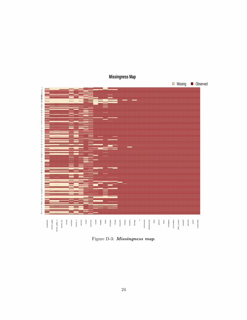
Next we multiply impute data to fill-in missing observations with imputed data. For thisanalysis, we restrict the sample to dictatorships, since the main findings pertain to autocracies andthe largest share of missing data is from autocracies. Figure D-3 shows the pattern of missingness forthe variables used in the multiple imputation algorithm. The five variables, depicted on the left sideof the horizontal axis, with the most missingness are all measures of remittance receipt. Movementrestrictions (l1move) and refugee flows (l1ref) also have substantial missingness, while population(l1pop), neighbor protest (l1nbr5), and net migration (l1migr) have very little missingness.
To assess whether missingness in the data – and the listwise deletion approach used in the maintext – biases estimates, we estimate again the main models reported in the text using multiplyimputed data. There are 2,650 observations in 104 countries with autocracies in the multiplyimputed data. The results are reported in Figure D-4. The top two estimates are from OLS and2SLS models with the same specification as used throughout, with the following baseline covariates:GDPpc, Population, Neighbor protest, Growth, Net migration, and Election period. The OLSestimate for Remittances is 0.113, which is slightly larger than the estimate with missing data forthe autocracies-only sample in Figure B-2 (0.102) and the interaction model in the main text, Table1, column 2 (0.086).
The 2SLS estimate using multiply imputed data, however, is substantially lower than the es-timate reported in the main text: 0.261 vs. 0.364. This difference suggests that using listwise
23
Missingness Map
tra
de
tax
rem
it_
gd
p
rem
it_
gd
p_
c
rem
it_
pc
rem
it
no
nta
x
rem
it_
c
taxre
v
l1re
f
l1m
ove
l1a
id
l1g
dp
l1ka
l1tr
ad
e
l12
gr
me
an
5
l1p
op
l1n
br5
l1m
igr s
rich
rem
it
dis
twre
mit
dis
t
ele
c3
ele
c
l1o
ilg
as
l1co
nflic
t
dis
t_co
ast
ca
se
id
pe
rio
d
ye
ar
cow
co
de
850840
830
820
816
812
811800790780
775771770
731712
710705704703702701700
698
696
690
678
670
663
652
651645640
630
625
620
616
615
600580
572
571570565560553552551
541
540531
530520
517516
510501
500
490484
483482
481475
471
461452451450
439
438
437436
435434433432
420404373372371370
365360355345339165160150145140135130101
9593929190704241
40
Missing Observed
Figure D-3: Missingness map.
24

deletion of missing data for the 2SLS approach biases the estimate upwards. This should not besurprising because much of the missing data on remittances is from prior to 1990, a period whenremittances from OECD countries – the basis for over-time variation in the excluded instrument– was relatively low compared with the post-1990 period. This means that the multiply imputeddata in the 2SLS approach is adding a substantial number of (instrumented) low-remittance ob-servations to the estimating sample, likely lowering the estimated correlation between remittancesand protest. Nonetheless, the 2SLS estimate using the baseline specification is large, positive andstatistically significant at the 0.05 level.
.272
.117
.245
.261
.113OLS
2SLS
2SLS exclude SSA
OLS + covariates
2SLS + covariates
0 .1 .2 .3 .4 .5Remittance estimate
Base covariates: GDPpc, Population, Neighbor protest, Growth, Net migration, ElectionAdditional covariates: Aid, Trade, KA open, Oil rents, Movement restrict., Refugee flows
Estimates from multiply imputed data
Figure D-4: Estimates from multiply imputed data.
The middle estimate reports the result from the baseline 2SLS model with multiply imputeddata but exclude SSA countries from the estimating sample. We conduct this test because thelistwise deletion strategy in the 2SLS model that drops SSA countries yields a relatively smallestimate (see Table C-2, column 6). Once we recover dropped observations from outside SSA, asreported here, the estimate for Remittances is roughly the same as the one that includes SSAcountries. However the variance estimate is considerably higher because dropping SSA countriesentails reducing the sample size by 44.5 percent – from 2,560 observations to 1,452. Thus it shouldnot be surprising that the variance is considerably larger.
The bottom two estimates reported in Figure D-4 repeat the OLS and 2SLS models withmultiply imputed data but include additional covariates, some of which have substantial missingdata: foreign aid, trade openness, KA (capital account) openness, oil and gas rents, movementrestrictions, and refugee flows. Including these additional covariates does not alter the estimatessubstantially: both the OLS and 2SLS estimates are positive and statistically significant.
25

R code for imputations
# g e t data ; miss mapdata . remit2<−read . dta ( ”temp mi2 . dta” )missmap (data . remit2 , c svar=”cowcode” , t sva r=” year ” , y . cex =0.4 , x . cex =.5)dev . copy2pdf ( f i l e=paste ( ” . /missmap” , ” . pdf ” , sep=”” ) )
# v a r i a b l e l i s t f o r a l l varsordvars<−c ( ” s ” , ” e l e c ” , ” e l e c 3 ” )keepvars<−c ( ”cow” , ” year ” , ” per iod ” , ” c a s e i d ” , ” remit ” , ” remit c” ,” remit gdp” , ” remit gdp c” , ” remit pc” , ” l1pop ” , ” l1gdp ” ,” l 1 a i d ” , ” l 1 t r a d e ” , ” l1migr ” , ” l 1 2g r ” , ” l 1 c o n f l i c t ” , ” l 1 o i l g a s ” , ” l 1 r e f ” ,” l1move” , ” l1ka ” , ” l1nbr5 ” , ” e l e c ” , ” e l e c 3 ” , ”mean5” ,” d i s t ” , ” d i s twremit ” , ” d i s t coas t ” , ” r i c h r e m i t ” , ” s ” )
# ID v a r i a b l e s to e x c l u d e from imputat ion modell a b e l v a r s<−c ( ” c a s e i d ” , ” per iod ” )
# impute miss ing v a l u e smy.m<−8my. idva r s<−l a b e l v a r simp . out<−amel ia ( x=data . remit2 , i dva r s=l a b e l v a r s , empri=7, p2s=2, m=my.m,ords=ordvars , c s=”cowcode” , ts=” year ” , i n t e r c s=TRUE, polyt ime =3)out1<−write . amel ia ( imp . out , f i l e . stem=” remit2imp ” , format=” dta ” )
26

Appendix E: Afrobarometer data
To measure the concept of geographic support for the incumbent government (progovern-ment) we use information on individual-level trust in the incumbent government and presidentialperformance ratings to construct a regional-level and a district-level measure of support for theincumbent. This Appendix contains the following additional analysis:
• information on individual-level non-response for sensitive questions about party affiliation,party voting, and measures of trust in the incumbent government and presidential perfor-mance rating.
• regional and district coding for progoverment
• region-level robustness tests
• district-level robustness tests
• tests that address district-level selection and individual-level selectionincluding treatment effects models
27

Non-response
This section discusses non-response to questions about political affiliation. There are two questionsrelating to political affiliation that are likely sensitive in non-democracies: Q86: Feel close to
which party (party) and Q97: Vote for which party (vote). A substantial number of respon-dents did not answer these questions by naming a particular party, as shown in the left panel ofFigure E-1: over 38 percent do not respond to the party question and 24 percent do not respond tothe vote choice question. At the country level, the non-response rates are correlated with politicalfreedom in the sample of eight non-democracies. The right plot if Figure E-1 shows this for theparty question while the right plot of Figure 1 in the main text shows this for the vote choice ques-tion. Further, the non-response rates are an order of magnitude higher for these sensitive questionsthan for other demographic and behavioral variables in the survey.
Cellphone
Discusspolitics Remittances
Protest
Vote
Party
0
.1
.2
.3
.4
Non
-res
pons
e ra
te
Variables
Non-response rates in eight non-democracies
Botswana
Burkina Faso
Mozambique
Namibia
Tanzania
Uganda
Zambia
Zimbabwe
0
.2
.4
.6
Non
-res
pons
e ra
te
4 6 8 10 12 14Freedom House score (combined)
Partisan non-response and political freedom
Figure E-1: Non-response rates for vote choice and partisan choice.
These figures provide evidence that the level of non-response to sensitive questions in thesecountries during the 2008 survey period is not trivial. To explore non-response further we next ex-amine the correlates of non-response. In the main text, we stated that in the eight non-democraciesin the 2008 round of the Afrobarometer survey, a strong predictor of refusing to respond to thevote choice question is whether the survey respondent resides in an opposition region or district.
We approach this question by modeling a binary indicator of whether the respondent chose oneof the following responses when asked to state the name of the political party for which they vote(Q97: Vote for which party): “Would not vote”, “Refused to answer”, or “Don’t know”. Themodel specification includes all the covariates in the baseline model in the main text as well as avariable for urban residence and another for whether the respondent “feels close to a political party”(Q85: Close to political party). Importantly, this latter variable should capture partisanindividuals without tapping into partisan affiliation or affinity. That is, this question does not askabout the party to which the respondent “feels close”, only whether the respondent has affinity forsome political party.
The main explanatory variables, in separate specifications, are the continous region- and district-
28

level measures of opposition to the incumbent government (i.e. 1- progovernment). We estimatea random effects logit with either the region or the district as the cross-section unit, with robusterrors clustered on the same unit. We do not use a conditional logit (i.e. fixed effects) because thefixed unit effect is perfectly co-linear with region-level (or district-level) measure of opposition. Themodel estimates in Figure E-2 shown in red are those for models that include all survey respondents(N=10,643). The top red estimate is from a model that measures opposition at the region-level whilethe bottom red estimate uses the district-level. Importantly, these models account for individualpartisanship (Q85: Close to political party).
Another set of tests combines information about whether the respondent “feels close” to aparty and whether s/he refuses to answer the question identifying the party for which s/he votes tocapture the respondents who might feel afraid to state their true party preference even if s/he “feelsclose” to a political party. The blue estimates in Figure E-2 are thus from models that restrict theanalysis to those respondents who “feel close” to a political party. Again, being in an oppositionregion or district is strongly correlated with non-response even among partisan respondents.
Region-level opposition
District-level opposition
0 .5 1 1.5 2Coefficient estimate
All Only partisans
Opposition region/district & non-response
Figure E-2: Non-response for vote choice.
Finally, the left panel of Figure E-3 shows the estimated marginal effect of the covariates in thedistrict-level model that looks only at partisan individuals (i.e. those who “feel close to” a politicalparty). These marginal effects (and 95 percent confidence intervals) are from the lower blue esti-mate in Figure E-2 (non-response to the partisan vote choice question, district-level analysis, onlypartisan respondents). By far, the strongest predictor of non-response is residence in an oppositiondistrict. The right plot in Figure E-3 shows the marginal effects when using the party affiliationvariable (Q86: Feel close to which party), with a similar strong effect for opposition district.
These tests provide evidence consistent with the contention that citizens in opposition areasmay be more reluctant than those in progovernment areas to state their political preferences. Ifthis is the case, then survey questions that ask respondents about their political affiliation, votingintentions, and perhaps even their ethnicity may not be reliable (on their own) for inferring whichrespondents are political opponents (supporters) of the ruling regime in non-democracies.
29

-.05
0
.05
.1
.15
Mar
igna
l effe
ct o
n no
n-re
spon
se
Oppositiondistrict
Cell phone Urban Age Education Wealth Male Employment
Vote choice non-response
-.05
0
.05
.1
.15
Mar
igna
l effe
ct o
n no
n-re
spon
se
Oppositiondistrict
Cell phone Urban Age Education Wealth Male Employment
Party choice non-response
Figure E-3: Marginal effects for non-response models.
30

Coding progovernment areas
This section describes the coding for region- and district-level progovernment share. To constructthis measure, we first take three variables that measure support for the incumbent regime. Notethat the non-response rates (reported in the second column below) are relatively low whencompared with the politically sensitive questions that require respondents to identify affinity orvote choice for a particular politcal party (24 and 37 percent).
Non-response Item-scaleAfrobarometer question rate correlation Meana
Q49A: Trust president 3.7 0.80 0.35Q49E: Trust the ruling party 5.5 0.84 0.45Q70A: Performance: President 8.1 0.71 0.68
a treats non-response as non-affirmative; i.e. in the denominator.
We then dichotomize the responses. In doing so, we treat non-response as a non-affirmativeanswer along with “disapprove”/“just a little”, “strongly disapprove”/“not at all”. The affirmativeresponses – “approve”/“somewhat”, “strongly approve”/“a lot” – comprise the other value of thedichotomous variable. By grouping non-response with non-affirmative responses, we assume thatnon-responders are not regime supporters (i.e not progovernment).
Next we construct an individual-level scaled index, bounded at 0 and 1, using Cronbach’s alpha.The overall test scale for the index is 0.69. All three items are strongly correlated with the scaledindex (see third column above). Of the three items in the scale, Trust president has the lowestvalue, with just over one third of respondents (0.35) demonstrating progovernment support withtheir response. The item with the highest average value is Performance:President, just over two-thirds of respondents demonstrated progoverment support with their response to this question.
Finally, we create a district-level average (mean) of the scaled individual-level index. Thisdistrict-level measure is bounded at 0 and 1. Each respondent in a particular district is assignedthe same district-level value of progovernment support.
Districts (614) are nested within the larger region units (185).10 The left plot of Figure E-4 showsthe bivariate relationship between coding progrovernment support at the region- and district-levels.There is a strong correspondence, unsurprisingly. That said, there are some districts with more than60 percent progovernment support but that lie in a region with less than 40 percent progovernmentsupport. Conversely, there are some districts with less than 40 percent progovernment supportbut that lie in a region with more than 60 percent progovernment support. This means that someindividuals will be placed in a relatively progovernment region but a weakly progovernment district– and vice versa.
The right plot of Figure E-4 shows how the region-level coding and the district-level codingoverlap. In this plot, we define an opposition region as one in which (average) progovernmentsupport is less than 0.5; a progovernment region is one in which progovernment support is morethan 0.5. The plot shows the distribution of district-level progovernment values (red distribution)and opposition (blue distribution) regions. The mode, median, and mean of the blue distributionare further towards the low end of the progovernment district-level scale (horizontal axis), while
10In the estimating sample for the reported results there are 469 districts because some districts have no observedprotest and thus drop from the estimating sample. In robustness tests using a random effects logit estimator, whichyields similar results, the full 614 districts remain in the estimating sample.
31

0
.2
.4
.6
.8
1R
egio
n-le
vel p
rogo
verm
ent
0 .2 .4 .6 .8 1
District-level progovernment
0
1
2
3
Den
sity
of d
istri
cts
0 .2 .4 .6 .8 1
District level pro-regime share of respondents
Opposition region
Progovernment region
614 districts
Figure E-4: District-level progovernment support, by region.
the same statistics for the red distribution (districts in progovernment regions) is further to theright.
We have no a priori reason to believe that regions or districts are the best geographic unitfor measuring geographic distributional coalitions across eight non-democracies, some with verydifferent political regimes. We therefore present results from both levels of aggregation. When weturn to addressing selection effects in the last sub-section, we conduct this analysis at the smaller,district-level because the the reported tests in the main text, the district-level results are weaker.
32

Robustness tests for regional analysis
In this section we report estimates for the main explanatory variable of interest, Remittance receiptwhile using the region-level coding of progoverment support. In each plot in Figure E-5 we reportestimates for the remittance coefficient from split-sample tests: one estimate for opposition regionsin blue and another estimate for progovernment regions in red.11 Opposition regions are coded asthose with less than 0.5 progovernment support (on the 0,1 scale of average progoverment support),while progovernment regions are coded as those with more than 0.5 government support. Thehorizontal axis in each plot measures the size of the remittance coefficient. The vertical axis simplyorders the estimates from each of the two models reported in each plot. In all specifications (exceptin the top left plot), the specification includes the demographic and economic control variablesincluded in the baseline model reported in the main text.
The top left plot estimates a specification without the demographic or economic control vari-ables, while the top right plot shows results from a specification with three additional controlvariables: whether the respondent “feels close” to a political party; whether the respondent did notanswer the (partisan) vote choice question; and whether the respondent voted in the last election.These are intended to capture other aspects of political participation and potential non-responseto ensure that the reported pattern relates to protest and not just any type of political activity.
The second row left plot reports results from random effects estimators rather than fixed effectsmodels, while the second row right plot shows results when adding ethnic group fixed effects (andstill including region fixed effects). The third row left plot shows results from a (region) fixed effectsmodel with a binary remittance variable (rather than the ordered remittance measure used in mostother specification), while the third row right plot shows results when using an ordered protestdependent variable rather than a binary variable. In the latter, the estimator is an ordered logit.
The bottom row plots report results from splitting the sample in two different ways to ensurethat the main findings remain in the tails of the distribution for the district-level measure ofprogovernment. These tests show how remittances influence protest in districts with high andlow levels of district progovernment support. The left plot splits the sample to include regionsone standard deviation below the mean and one standard deviation above the mean, leaving outdistricts in the middle of the distribution. Similarly, the right plot splits the sample below the 25thpercentile and above the 75th percentile of the region-level measure of progovernment distribution,leaving out districts in the middle 50 percent of this distribution.
In all these tests, a familiar pattern emerges: remittances are positively associated with protestin opposition regions but not in progovernment regions.
11In the replication materials, we estimated the interaction models with similar results.
33

-.1 0 .1 .2 .3
Opposition
Progovernment
No controls
-.1 0 .1 .2 .3
Opposition
Progovernment
More controls
-.1 0 .1 .2
Opposition
Progovernment
Random effects
-.1 0 .1 .2 .3
Opposition
Progovernment
Ethnic group fixed effects
-.2 0 .2 .4 .6
Opposition
Progovernment
Binary remittance variable
-.1 -.05 0 .05 .1
Opposition
Progovernment
Ordered protest variable
-.2 -.1 0 .1 .2
Opposition
Progovernment
Cut-point: +- 1 Stdev
-.2 -.1 0 .1 .2 .3
Opposition
Progovernment
Cut-point: 25pctle, 75pctile
Coefficient estimates for Remittances
Regional coding
Figure E-5: Region-coding robustness tests.
34

Robustness tests for district-level analysis
In this section we report estimates for the main explanatory variable of interest, Remittance receiptwhile using the district-level coding for progovernment. In each plot in Figure E-6 we reportestimates for the remittance coefficient from split-sample tests: one estimate for opposition districtsin blue and another estimate for progovernment districts in red.12 In this set of tests, we defineopposition as any district where the district-level progovernment mean is less than or equal to 0.5;we define progovernment as any district where the district-level progovernment mean is greater than0.5. We vary this cut-point of 0.5 in the latter two sets of models (see below). The horizontal axisin each plot measures the size of the remittance coefficient. The vertical axis simply orders theestimates from each of the two models reported in each plot. In all specifications (except in thetop left plot), the specification includes the standard demographic and economic control variables.
The top left plot estimates a specification without the demographic or economic control vari-ables, while the top right plot shows results from a specification with three additional controlvariables: whether the respondent “feels close” to a political party; whether the respondent did notresponse the (partisan) vote choice question; and whether the respondent voted in the last election.These are intended to capture other aspects of political participation and interest to ensure thatthe reported pattern relates to protest and not just any type of political activity.
The second row left plot reports results from random effects estimators rather than fixed effectsmodels, while the second row right plot shows results when adding ethnic group fixed effects (andstill including district fixed effects). To obtain convergence in this model with district fixed effects,we add ethnic-group means (as an ethnic-group FE proxy) for all covariates and the dependentvariable.13 The third row left plot shows results from a (district) fixed effects model with a binaryremittance variable (rather than the ordered remittance measure used in most other specifications),while the third row right plot shows results when using an ordered protest dependent variable ratherthan a binary variable. In the latter, the estimator is a random effects ordered logit.14
Finally, the bottom row plots report results from splitting the sample in two different ways toensure that the main findings remain in the tails of the distribution for the district-level measureof progovernment. These tests show how remittances influence protest in districts with high andlow levels of district progovernment support. The left plot splits the sample to include districtone standard deviation below the mean and one standard deviation above the mean, leaving outdistricts in the middle of the distribution. Similarly, the right plot splits the sample below the 25thpercentile and above the 75th percentile of the district-level measure of progovernment distribution,leaving out districts in the middle 50 percent of this distribution.
In all these tests, a familiar pattern emerges: remittances are positively correlated with protestin opposition regions but not in progovernment regions.
12In the replication materials, we estimated the interaction models with stronger results.13Recall that there are 469 districts in the conditional logit sample.14A district fixed effects estimator does not converge in split-samples, so we estimate a district-random effects
model with the district-level mean of progovernment as covariate to properly estimate the interaction specification.
35

-.05 0 .05 .1 .15 .2
Opposition
Progovernment
No controls
-.1 0 .1 .2
Opposition
Progovernment
More controls
-.1 -.05 0 .05 .1 .15
Opposition
Progovernment
Random effects
-.1 0 .1 .2
Opposition
Progovernment
Ethnic group fixed effects
-.2 0 .2 .4 .6
Opposition
Progovernment
Binary remittance variable
-.05 0 .05 .1
Opposition
Progovernment
Ordered protest variable
-.1 0 .1 .2 .3
Opposition
Progovernment
Cut-point: +- 1 Stdev
-.2 -.1 0 .1 .2 .3
Opposition
Progovernment
Cut-point: 25pctle, 75pctile
Coefficient estimates for Remittances
District coding
Figure E-6: District-coding robustness tests.
36

Full sampleestimateFull sample
estimate
0
1
2
3
4
5
-.05 0 .05 .1 .15 .2
βRemittances
Low progovt. High progovt.
Region-level
Figure E-7: Region-level. Leave-one-country-out.
Full sampleestimate
Full sampleestimate
0
1
2
3
4
5
-.05 0 .05 .1 .15 .2
βRemittances
Low progovt. High progovt.
District-level
Figure E-8: District-level. Leave-one-country-out.
Figures E-7 and E-8 shows the estimates for Remittances at low (10th percentile, in red) andhigh (90th percentile, blue) levels of progovernment support when we drop one country at a time.In each plot, the horizontal axis measures the estimated coefficient for Remittances; the verticleaxis measures the frequency of the estimates. The plots also show the estimate from the full sampleestimate. The reported estimates from the full sample do not differ appreciably from the leave-one-out estimates. For interested readers, we note that the results are weakest (though still statisticallysignificant) when we drop Uganda from the sample and strongest when we omit Zimbabwe.
37

Addressing selection effects
Throughout the paper, we posit that remittances increase protest by increasing opposition re-sources. In this section, we address alternative mechanisms that might also give rise to a positiveassociation between remittances and protest that is strongest in opposition areas.
Geographic (district-level) selection If protests are more likely to occur in opposition areas,there is more location-based opportunity for people to participate in protests. And if citizens inopposition areas receive more remittances, then a finding that remittances increase protest might bespurious insofar as it could simply indicate that grievances drive emigration (and hence remittances)from particular districts as well as protest opportunity in those districts.
This alternative focuses on heterogeneity in geographic place; that is, protest opportunity basedon location is an unobserved factor related to protest and remittances. Our empirical approachdirectly addresses this concern (and other location-based unobserved factors) by using a fixedeffects estimator, which models all cross-section heterogeneity. The conditional logit (with groupeffects for district) addresses this alternative logic because the estimator compares individuals withremittances in district d to those without remittances in the same district d; that is, individualsare compared to others within the same district. The estimator then calculates the (weighted)average of these individual-level comparisons within each district, for all districts. The estimatorthus directly models location-based differences that shape protest opportunity structure, includinggeographic differences in access to public goods, maltreatment by the government, ethnicity, thelocal history of protest mobilization, and the mobilization efforts of opposition groups. We chosethis estimator over others (such as a random-effects estimator) for precisely this reason.
That said, we may still want to see the distributions of observed protest and remittance receiptacross different district levels of government support.15 Figure E-9 shows these distributions. Theleft panel shows the fraction of protesters and non-protesters for different district levels of pro-government support. Comparing the blue histogram (protesters) with the red-outlined histogram(non-protesters) shows that in districts with low levels of government support (i.e. opposition dis-tricts) non-protestors generally outnumber protestors. In districts with medium to high levels ofgovernment support (strongholds), protestors generally outnumber non-protestors. The relation-ship between district-level progovernment support and individual protest can be summarized bylooking at the local area regression line, which is slightly positive (up to 0.8 level of progovern-ment support). This suggests that individual protest is more likely in progovernment districts thanin opposition districts – except in highly progovernment areas (i.e. with progovernment supportgreater than 0.8).
The right panel of Figure E-9 shows the fraction of remittance recipients and non-recipientsfor each level of district progovernment support. There is a strong negative relationship betweendistrict-level progrovernment support and remittance receipt: opposition districts have a highershare of remittance recipients than stronghold districts.
This analysis indicates that district-level progovernment support is positively correlated withprotest but negatively correlated with remittance receipt. This evidence is not consistent with thealternative logic, which posits that opposition districts provide more protest opportunity. As im-portant, the statistical relationship between district-level progovernment support and the outcome
15Recall that the district level of government support is the average individual level of progovernment across allrespondents in each district.
38

0
.1
.2
.3
.4
0
.02
.04
.06
Indi
vidu
al p
rote
st
0 .2 .4 .6 .8 1District-level progovenment support
ProtestNot protestLocal arearegression
Protest
0
.1
.2
.3
.4
0
.02
.04
.06
Indi
vidu
al re
mitt
ance
rece
ipt
0 .2 .4 .6 .8 1District-level progovenment support
Remittance receiptNo remittancesLocal arearegression
Remittance receipt
Figure E-9: Protest and remittance receipt by district-level progovernment support.
variable (individual protest) and the relationship between district-level progovernment support andthe main explanatory variable (individual remittance receipt) is modeled in the analysis when weemploy the conditional logit estimator. That is, the empirical relationships observed in E-9 are di-rectly modeled in the analysis. These relationships are not omitted factors in the analysis. Rather,the estimates we report in the main text account for all the ways district-level differences in emigra-tion patterns, grievances, government efforts to thwart remittance receipt, and protest opportunitystructure influence the individual-level outcome and individual-level explanatory variables.
Individual-level selection Unmodeled individual differences could plausibly account for therelationship between emigration (and hence remittances) and protest. Individuals from more risk-accepting families, for example, may be more likely to emigrate and more likely to protest. Thatis, if risk-acceptant families have one member who migrates abroad and another who protests,then family-level risk-acceptance differences could yield a positive statistical relationship betweenremittances and protest at the individual-level that has nothing to do with family resources. Forthis type of individual-level selection effect to account for our findings, however, the selection effectwould have to operate more strongly in opposition districts than in progovernment districts.
Our analysis cannot account for all of the possible individual-level differences that might causea spurious relationship between remittances and protest. In the analysis reported in the maintext we account for demographic and economic differences among individuals, such as age, gender,educational attainment, employment status, and wealth. We also account for self-reported traveland cellphone acccess, as these individual characteristics are additional plausible confounders.
To further address individual-level selection, in this section we add four distinct types ofindividual-level confounders that are related to different sources of “grievance”. If aggrieved re-spondents are more likely to protest, more likely to receive remittances, and more likely to residein opposition districts, then this unobserved individual-level factor could cause the model to yield
39

upwardly biased estimates of the relationship between remittances and protest.We model four distinct (possible) sources of individual-level grievance: anti-government sen-
timent; material deprivation; fear of the regime; and paying bribes. The first source of grievancecaptures individual-level sentiment towards the incumbent national government and thus accountsfor the possibility that the government targets particular individuals based on their individual-levelprogovernment sentiment. Antigovernment individuals, for example, may be more likely targetsof government efforts to stymie remittances flows to political opponents. The second source ofgrievance, relative material deprivation, accounts for the possibility that individuals who have lessmaterial goods than others in their country are more likely to emigrate and to protest. The thirdsource of grievance is fear of the regime, which accounts for the possibility that individuals alreadytargeted by the government as known opponents are more likely to come from families that haveemigrants members and that are more likely to protest. These individuals may also be targetsof government efforts to deter remittance receipt. Finally, corruption – one manifest indicator ofwhich is paying bribes – is a potential source of individual grievance (Hiskey, Montalvo and Orces,2014). If individuals who experience more corruption are more likely to seek out remittances andto protest, this could confound the micro-analysis.
The individual-level measure of anti-government sentiment is simply the inverse of theindividual-level progovernment variable constructed for the district-level progovernment variable.Since this index aggregates information from questions that pertain to national leadership, we stan-dardize it by country by subtracting the country mean from the individual-level index. Absolutematerial deprivation is an index that combines information on questions about lack of access to cleanwater, food, and medicine. Relative deprivation is the absolute deprivation minus the country meanlevel of absolute deprivation. Fear of the regime is a latent index derived from four questions on thesurvey that tap into fears about political participation: Q46. How often careful what you say;Q47. How much fear political intimidation and violence; Q48A. How likely powerful
find out your vote; and Q48B. How likely punishment for making complaints. Again, wecalculate relative fear by substracting the country average level of fear from the index. Finally, wemeasure grievance based on corruption from three questions about self-reported behavior of payingbribes: to obtain a document or permit (Q51A); to obtain water or sanitation services (Q51B); or toavoid a problem with the police (Q51C).
To investigate whether these individual-level sources of potential grievance are confounders,we test models with these variables – both individually and all together. Figure E-10 reportsestimates for these variables from a conditional logit specification with the full set of individual-level demographic variables. The left plot shows the estimates from a model where the outcomevariable is protest participation; remittance receipt is not in the specification. The first four modelsinclude each of the four types of grievance indicators one at a time, while the fifth set of estimates –shown with a black triangle – is from a specification that includes all four indicators. Paying bribesis strongly correlated with protest, but the other three types of individual sources of grievance arenot. The right panel repeats this exercise but employs remittance receipt as the outcome variable.Again we find evidence that bribes are associated with remittance receipt. There is also someevidence that fear – at least as we have measured it here – is correlated with remittance receipt.This suggests that bribe paying and perhaps fear are individual-level confounders that tap intoindividual-level grievances.
Next we test the main specification from the main text with protest as the outcome variable andthe full set of demographic controls, with results reported in Figure E-11. Protest is the dependent
40

Bribe
Fear
Anti-govt
Deprivation
-1 -.5 0 .5 1Coefficient estimate
Protest
Bribe
Fear
Anti-govt
Deprivation
-1 -.5 0 .5 1Coefficient estimate
Remittance receipt
Control variables in specification but not shown
Figure E-10: Individual-level grievance, protest, and remittances.
Remit
Remit x Progov
Bribe
Fear
Anti-govt
Deprivation
-.5 0 .5 1 1.5 Control variables in specification but not shown
Protest
Figure E-11: Including individual-level grievance as confounders in the main specifica-tion.
41

variable and remittance receipt is the main explanatory variable. We add each individual-levelgrievance indicators to the specification, one at a time. The last model, shown with black triangles,includes all four grievance indices. The main result for remittances and the interaction betweenremittances and progovernment district remains robust in all specifications. We also find that bribepaying is positively associated with protest.
The results reported in Figures E-10 and E-11 indicate that the main findings cannot be at-tributed to individual-level grievances – at least as measured by the indices we have constructedhere. Given the data available from this survey, we have attempted to account for individual-levelgrievance as a confounder that causes individual-level selection into both protest and remittancereceipt. This did not change the main findings.
This analysis, however, cannot account for all individual- or family-level factors that may causeboth protest and emigration, such as risk acceptance or human capital potential. A design thatcould capture all such individual attributes would have to be a longitudinal panel that queries thesame individuals repeatedly over time with sufficient variation in both protest participation andremittance receipt over time within individuals.16 To our knowledge, no such survey exists forrespondents living in a non-democracy.
Treatment effects model In this section, we estimate a treatment effects model for observa-tional studies that matches treated observations (i.e. individuals who receive remittances) withun-treated observations (i.e. individuals who do not receive remittances) who have similar at-tributes on potential confounding variables. If we believe that, conditional on the covariates in themodel, treatment assignment (i.e. probability of receiving remittances) does not influence the po-tential outcome (i.e. participating in a protest), then the results of this analysis can be interpretedas causal. In this application, we acknowledge that there may be unmodeled potential confounders,such as individual- or family-level risk acceptance – that influence both treatment assignment andthe potential outcome.
First we employ coarsened exact matching (CEM), which attempts to match treated ob-servations with untreated observations with the same values on the confounding variables(Iacus, King and Porro, 2012). Once the matched data are identified, we compare the mean valuesof the outcome for treated and control groups as well as estimate a model of protest using thetrimmed data set of matched observations.
CEM attempts to match observations on exact values of the confounders. For a dichotomousvariable, such as male in our application, CEM matches observations with the same values, i.e.matches males with males and females with females. For ordered variables, such as education inour application, we use CEM to match on exact values. For continous confounders, however, webin the data to create ordered values for matching (Blackwell et al., 2009). Binning values of acontinuous variable in ordered categories coarsens the data.
In this application, there is a trade-off between achieving balance between treated and con-trol observations and trimming the data set too much such that the matching yields a rel-atively small number of matched treated observations and thus creates inefficient estimates(Iacus, King and Porro, 2012, 13). We match on all the baseline demographic confounders (age,gender, employment, wealth, and education), two behavioral confounders (cellphone use and travel)and two grievance measures. Because bribes empirically confounds, as shown in the previous sec-
16Further, sampling would have to account for individual-level attrition over time and the questionaire would haveto include items that could be used to model the attrition.
42
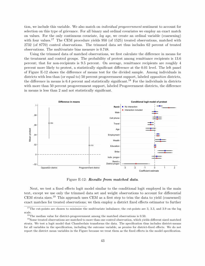
tion, we include this variable. We also match on individual progovernment sentiment to account forselection on this type of grievance. For all binary and ordinal covariates we employ an exact matchon values. For the only continuous covariate, log age, we create an ordinal variable (coarsening)with four values.17 The CEM procedure yields 950 (of 1525) treated observations, matched with2732 (of 8770) control observations. The trimmed data set thus includes 62 percent of treatedobservations. The multivariate bias measure is 0.748.
Using the trimmed data of matched observations, we first calculate the difference in means forthe treatment and control groups. The probability of protest among remittance recipients is 13.6percent; that for non-recipients is 9.5 percent. On average, remittance recipients are roughly 4percent more likely to protest, a statistically significant difference at the 0.01 level. The left panelof Figure E-12 shows the difference of means test for the divided sample. Among individuals indistricts with less than (or equal to) 50 percent progovernment support, labeled opposition districts,the difference in means is 6.4 percent and statistically significant.18 For the individuals in districtswith more than 50 percent progovernment support, labeled Progovernment districts, the differencein means is less than 2 and not statistically significant.
.064
.019
-.02
0
.02
.04
.06
.08
.1
Mea
n pr
otes
t
Opposition district Progovernment district
Difference in means
Remit
Male
Cell phone
Travel
Age
Employment
Wealth
Education
Bribe
Indiv. progov
Remit xDistrict progov
-3 -2 -1 0 1 2Coefficient estimate
No interactionInteraction included
Conditional logit model of protest
Figure E-12: Results from matched data.
Next, we test a fixed effects logit model similar to the conditional logit employed in the maintext, except we use only the trimmed data set and weight observations to account for differentialCEM strata sizes.19 This approach uses CEM as a first step to trim the data to yield (coarsened)exact matches for treated observations; we then employ a district fixed effects estimator to further
17The cut-points are chosen to minimize the multivariate imbalance; the cut-points are 3, 3.3, and 3.9 on the logscale.
18The median value for district-progovernment among the matched observations is 0.50.19Some treated observations are matched to more than one control observation, which yields different sized matched
strata. We test a logit model that Chamberlain transforms the data. The specification thus includes district-meansfor all variables in the specification, including the outcome variable, as proxies for district-fixed effects. We do notreport the district mean variables in the Figure because we treat them as the fixed effects in the model specification.
43

account for geography-based selection issues (Iacus, King and Porro, 2012, 3). Importantly, oneof the mean variables in the Chamberlain transformed data is the district-mean of progovernmentsupport. This variable captures all district-level differences in protest opportunity structure.
The results of this analysis are reported in the right panel of Figure E-12. First, we test amodel without the interaction between remittance receipt and district progovernment sentiment.This model, shown in blue •’s, yields a positive and significant estimate for Remit. Next we includethe interaction term in the specification, shown in red 4’s. The estimate for Remit, which is themarginal effect when district progovernment is set to zero, is positive and statistically significant.The estimate for the interaction is negative and significant. This indicates that remittances arepositively associated with protest in opposition districts – those with little progoverment support.But this positive effect becomes smaller and approaches zero as district-level progovernment supportincreases.
In replication files, we repeat the CEM plus fixed effects logit approach shown in the right panelof Figure E-12, but alternatively substituted fear and relative deprivation for bribes in the matchingprocedure. We find similar results.
Finally, in replication files we use the CEM approach to create a trimmed matched data setfor split samples and then estimate a fixed effects logit model with the trimmed data. First wesplit the sample into two bins: districts with less than (or equal to) 50 percent progovernmentsupport (Opposition districts) and districts with greater than 50 percent progovernment support(Progovernment districts). Then we use CEM to match observations, creating a separate trimmeddata set for Opposition and Progovernment groups of districts. Then we estimate fixed effectslogit models (with Chamberlain transformations of the data). This analysis yields almost identicalresults: the estimate for Remittances in Opposition districts is positive and significant, while theestimate for Remittances in Progovernment districts is negative but not statistically significant.
References
Abdih, Yasser, Ralph Chami, Jihad Dagher and Peter Montiel. 2012. “Remittances and Institutions:Are Remittances a Curse?” World Development 40(4):657–666.
Blackwell, Matthew, Stefano M. Iacus, Gary King and Giuseppe Porro. 2009. “CEM: CoarsenedExact Matching in Stata.” The Stata Journal 9(4):524–546.
Chenoweth, Erica, Vito D’Orazio and Joseph Wright. 2014. “A Latent Measure of Political Protest.”Paper presented at the International Studies Association’s 55th Annual Convention, Toronto(Canada), March 26-29.URL: http://sites.psu.edu/wright/files/2017/09/CDW-Protest1-239iz5j.pdf
Chinn, Menzie D. and Hiro Ito. 2008. “A New Measure of Financial Openness.” Journal of Com-parative Policy Analysis 10(3):309–322.
Cingranelli, David L., David L. Richards and K. Chad Clay. 2014. “The CIRI Human RightsDataset.”. Version 2014.04.14.URL: http://www.humanrightsdata.com
Garreton, Manuel Antonio. 1988. “Popular Mobilization and the Military Regime in Chile: TheComplexities of the Invisible Transition.” Kellogg Institute for International Studies, Working
44

Paper # 103.URL: https://kellogg.nd.edu/documents/1297
Gleditsch, Nils Petter, Peter Wallensteen, Mikael Eriksson, Margareta Sollenberg and HavardStrand. 2002. “Armed Conflict 1946-2001: A New Dataset.” Journal of Peace Research 39(5):615–637.
Hainmueller, Jens and Chad Hazlett. 2013. “Kernel regularized least squares: Reducing misspec-ification bias with a flexible and interpretable machine learning approach.” Political Analysis22(2):143–168.
Hainmueller, Jens, Jonathan Mummolo and Yiqing Xu. 2016. “How Much Should We Trust Es-timates from Multiplicative Interaction Models? Simple Tools to Improve Empirical Practice.”Working Paper, available at: http://bit.ly/2awUS3M.
Hiskey, Jonathan, Jorge D. Montalvo and Diana Orces. 2014. “Democracy, Governance, and Em-igration Intentions in Latin America and the Caribbean.” Studies in Comparative InternationalDevelopment 49(1):89–111.
Iacus, Stefano M., Gary King and Giuseppe Porro. 2012. “Causal Inference without BalanceChecking: Coarsened Exact Matching.” Political Analysis 20(1):1–24.
Nunn, Nathan and Diego Puga. 2012. “Ruggedness: The blessing of bad geography in Africa.”Review of Economics and Statistics 94(1):20–36.
Ross, Michael and Paasha Mahdavi. 2015. “Oil and Gas Data, 1932-2014.”.URL: http://dx.doi.org/10.7910/DVN/ZTPW0Y
World Bank. 2011. Migration and Remittances Factbook [2nd Edition]. Washington, DC: WorldBank.
45