On the Turbulent Mixing and Ozone Variations in the Tropical Tropopause Layer associated with Kelvin Waves

1. Introduction 2. Data

References

TTL workshop

4. Results in the height & isentropic coordinates

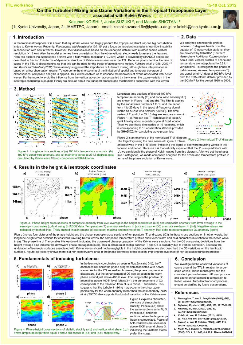
5. Fundamentals of inducing turbulence

Figure 2. Normalized T’-U’ diagram.

3. Method

Figure 1. Longitude time sections of (a) 100 hPa temperature anomaly , (b)

100 hPa zonal wind anomaly, and (c) their time series at 271.5 degrees east

calculated by Kelvin wave filtered component of ERA-Interim.

In the tropical atmosphere, it is known that equatorial waves can largely perturb the tropopause structure; one big perturbation

is due to Kelvin waves. Recently, Flannaghan and Fueglistaler (2011)1 put a focus on turbulent mixing by shear-flow instability

in connection with Kelvin waves. However, their discussion is based on the reanalysis dataset with a rather coarse vertical

resolution (~1.5 km). Also the model schemes have uncertainty, thus the observational study needs to assess the features.

Here, we explore the ozonesonde archive with a high vertical resolution (~0.2 km) which is provided by SHADOZ project (as

described in Section 2) in terms of dynamical structure of Kelvin waves seen near the TTL. Because photochemical life time of

ozone in the TTL is about months, so that this can be used for the tracer of atmospheric motion. Fujiwara et al. (1998, 2003)2,3

and Koishi and Shiotani (2012)4 have already suggested the importance of turbulent mixing, although their interpretation is

based on a few observation results. To overcome the shortcoming of the limitation of spatial and temporal coverage of

ozonesondes, composite analysis is applied. This will be enables us to describe the behaviors of ozone associated with Kelvin

waves. Furthermore, to avoid the influence from the vertical advection accompanied by the waves, the ozone variation in the

isentropic coordinate is studied. Finally we discuss about the transport process and mechanisms associated with the waves.

Longitude-time sections of filtered 100 hPa

temperature anomaly (T’) and zonal wind anomaly (U’)

are shown in Figure 1 (a) and (b). The filter is applied

by the zonal wave numbers 1 to 10 and the period

from 4 to 23 days in the spectral-frequency domain

(same as Suzuki and Shiotani (2008)5). The time

series of T’ and U’ at 271.5 degrees east are shown in

Figure 1 (c). We can see T’ (light blue line) leads U’

(pink line) by about a quarter cycle at fixed location.

Then we use these time series at 10 locations, which

is corresponding to 10 observation stations provided

by SHADOZ, for calculating wave properties.

We analyzed ozonesonde profiles

between 10 degrees bands from the

equator of 10 observation stations; they

are provided by SHADOZ (Southern

Hemisphere Additional Ozonesondes).

About 3000 vertical profiles of ozone and

temperature are interpolated to 0.2 km

vertical bins. To categorize the phase of

Kelvin waves, we used temperature (T)

and zonal wind (U) data at 100 hPa level

from the ERA-Interim dataset provided by

the ECMWF for the period 1998 to 2009.

Figure 4. Phase-height cross sections of statistic stability (a,b) and vertical wind shear (c,d).

Wave amplitude larger than equal 1 and 2 are shown in (a,c) and (b,d), respectively.

Figure 2 is an example of the normalized T’-U’ diagram.

The trajectory using the time series of Figure 1 rotates

We investigated the observed variations of

ozone around the TTL in relation to large-

scale waves. These results provided the

consistent picture between diffusion process

and ozone enhancement in connection to

Kelvin waves. Turbulent transport process

should be clarified by future observations.

anticlockwise in the T’-U’ plane, indicating the signal of eastward traveling waves in this

location and period. Because it is theoretically expected that the T' is in quadrature with

U', we can identify the phase of Kelvin waves from this diagram. After we put the phases

into 8 categories, we made composite analyses for the ozone and temperature profiles in

terms of the phase evolution of Kelvin wave.

Kazunari KOISHI 1, Junko SUZUKI 2, and Masato SHIOTANI 1

(1: Kyoto University, Japan, 2: JAMSTEC, Japan) email: koishi.kazunari.6v@kyoto-u.ac.jp or koishi@rish.kyoto-u.ac.jp

1. Flannaghan, T. and S. Fueglistaler (2011), GRL,

38, doi:10.1029/2008GL033641.

2. Fujiwara, M., et al. (1998), JGR, 103, 19173-19182.

3. Fujiwara, M., et al. (2003), GRL, 30,

doi:10.1029/2002Gl016278.

4. Koishi, K., and M. Shiotani (2012), JMSJ,

90, No.3, 403-416, doi:10.2151/jmsj.2012.304.

5. Suzuki, J., and M. Shiotani (2008), JGR, 113,

doi:10.1029/2007JD009456.

6. Nishi, N., J. Suzuki, A. Hamada, and M. Shiotani

(2007), SOLA, 3, 13-16, doi:10.2151/sola.2007-004.

15-19 Oct. 2012

12

3

4

56

7

8

6. Conclusion

Figure 3 show four pictures of the phase-height and the phase-isentropic cross sections of temperature (T) and ozone (O3). In these cross sections or, in other words, the

longitude-height cross sections for eastward traveling Kelvin waves, the composite temperature profiles show clear warm and cold anomalies in relation to the Kelvin wave

in (a). The phase line of T anomalies tilts eastward, indicating the downward phase propagation of the Kelvin wave structure. For the O3 composite, deviations from the

height average also indicate the downward phase propagation in (b). This in-phase relationship between T and O3 is probably due to vertical advection. Because the

undulation of isentropic surfaces associated with Kelvin waves should not be negligible in the height coordinate, we also described the O3 variations on the isentropic

surfaces. Figure 3(d) clearly shows there is a non-conservative area in the phase-isentropic cross section, implying the evidence of non-adiabatic transport process.

Figure 3. Phase-height cross sections of composite anomaly from level average in the height coordinates (a,b) and composite anomaly from level average in the

isentropic coordinates (c,d) all using SHADOZ data. Temperature (T) anomaly are drawn in (a,c) and ozone (O3) anomaly are drawn in (b,d). Negative values are

indicated by dashed lines. Thick dashed lines in (c) and (d) represent maxima and minima of the T anomaly. Red color represents positive O3 anomaly [ppbv].

a) b) c) d)

a) b)

c) d)

In the isentropic coordinates as seen in Figs.3(c) and 3(d), the T

anomalies still show the phase progression associated with Kelvin

waves. As for the O3 anomalies, however, the phase progression

disappears, but the enhancement of O3 can be seen in the warm

phase around just above 400 K level. Focusing on the positive O3

anomalies above 400 K level (phase3-4), the enhancement of O3

corresponds to the transition from plus to minus T anomalies. This

suggests that the turbulent mixing may occur in the shear zone

particularly for the warm anomaly rather than the cold anomaly. Nishi

et al. (2007)6 also supports this kind of transition of the Kelvin waves.

amp.

time

T’- O3’+ T’+

a) b) c)

phasephasephase

phase 3

phase 3

phase

phase

shear zone

Figure 4 explores characteri-

cteristics of atmospheric

stability. Panels (a,c) show

the same sections as in Fig.3.

Panels (b,d) show the

sections, when the large amp-

litude is categorized. Peaks of

both variables are seen near

above 400K around phase 3,

indicating the unstable states

prefer this stage.

phase8 4 8 48 48 4