turbulent mixing in a stratified fluidmaecourses.ucsd.edu/groups/linden/pdf_files/74hl99.pdf ·...

Dynamics of Atmospheres and OceansŽ .30 1999 173–198

www.elsevier.comrlocaterdynatmoce

Turbulent mixing in a stratified fluid

Joanne M. Holford ), P.F. Linden 1

Department of Applied Mathematics and Theoretical Physics, UniÕersity of Cambridge, SilÕer Street,Cambridge, England CB3 9EW, UK

Received 22 September 1998; received in revised form 10 May 1999; accepted 28 June 1999

Abstract

The strength of diapycnal mixing by small-scale motions in a stratified fluid is investigatedthrough changes to the mean buoyancy profile. We study the mixing in laboratory experiments inwhich an initially linearly stratified fluid is stirred with a rake of vertical bars. The flow evolution

Ž .depends on the Richardson number Ri , defined as the ratio of buoyancy forces to inertial forces.At low Ri, the buoyancy flux is a function of the local buoyancy gradient only, and may bemodelled as gradient diffusion with a Ri-dependent eddy diffusivity. At high Ri, vertical vorticityshed in the wakes of the bars interacts with the stratification and produces well-mixed layersseparated by interfaces. This process leads to layers with a thickness proportional to the ratio of

Ž .grid velocity to buoyancy frequency for a wide range of Reynolds numbers Re and gridsolidities. In this regime, the buoyancy flux is not a function of the local gradient alone, but alsodepends on the local structure of the buoyancy profile. Consequently, the layers are not formed bythe PhillipsrPosmentier mechanism, and we show that they result from vortical mixing previouslythought to occur only at low Re. The initial mixing efficiency shows a maximum at a critical Riwhich separates the two classes of behaviour. The mixing efficiency falls as the fluid mixes and asthe layered structure intensifies and, therefore, the mixing efficiency depends not only on theoverall Ri, but also on the dynamics of the structure in the buoyancy field. We discuss someimplications of these results to the atmosphere and oceans. q 1999 Elsevier Science B.V. Allrights reserved.

Keywords: Turbulent mixing; Stratified fluid; Buoyancy

) Corresponding author. Tel.: q44-1223-337858; fax: q44-1223-3379181 Present address: Department of Mechanical and Aerospace Engineering, University of California, San

Diego, 9500 Gilman Drive, La Jolla, CA 92093-0411, USA.

0377-0265r99r$ - see front matter q 1999 Elsevier Science B.V. All rights reserved.Ž .PII: S0377-0265 99 00025-1

( )J.M. Holford, P.F. LindenrDynamics of Atmospheres and Oceans 30 1999 173–198174

1. Introduction

In nature, most fluids are perturbed by motions on a wide range of scales. Whilesystematic flows on larger scales can be calculated directly, smaller turbulent motionsoccur below the resolution of most numerical models. These small-scale motions areimportant, both as a sink of large-scale energy and through enhanced transport ofpassive scalars, buoyancy and momentum. In this study, the transport of buoyancy in aparticular turbulent field in a stratified fluid is investigated.

In an unstratified turbulent fluid, the mean flux q of a passive scalar s iss

proportional to the mean concentration gradient, q syK =s, for times large compareds sŽ Ž . Ž ..to the Lagrangian timescale of the turbulence Taylor 1915 ; Batchelor 1949 . The

constant of proportionality, K , known as the eddy diffusivity, can be expressed in termssŽ .of the time rate of change of root mean square rms particle displacements and, in

homogeneous isotropic turbulence, is approximately equal to the product of the turbulentintegral lengthscale and the rms turbulent velocity.

Stable stratification affects the flow in several ways. Vertical mixing of the stratifica-tion provides an additional sink of energy. The stratification also influences the structureof the turbulence, since vertical motions are directly affected by buoyancy forces.Turbulence in a stratified fluid is typically anisotropic, with reduced vertical velocitiesand vertical lengthscales, and a reduced correlation between the density perturbation andthe vertical velocity component, as seen, for example, in the stratified flume experiments

Ž .of Stillinger et al. 1983 . Horizontal motions organise into vortical structures, whichŽ .then cascade energy to larger scales. The experiments of Fincham et al. 1994 , in which

the decaying wake behind a rake of vertical bars towed once through a stratified fluidwas observed, exemplify this flow regime, which is ultimately dominated by aninteracting field of large aspect ratio ‘‘pancake’’ vortices at different levels.

The concept of turbulent gradient diffusion may be extended to weakly stratifiedfluids by allowing the eddy diffusivity to vary with the local buoyancy gradient N 2. For

Ž .example, Noh and Fernando 1995 use an eddy diffusivity based on the local turbulentŽ .kinetic energy TKE e, and a vertical mixing length which varies with local Richardson

number, Ri, taking the values l in an unstratified fluid and e1r2rN in a strongly0

stratified fluid.An overall measure of the mixing in a flow is the mixing efficiency h, here defined

Ž .as the ratio of the change in background potential energy PE of the fluid to the changeŽ .in available potential and kinetic energy. The mixing efficiency lies in the range

0FhF1, and all input energy not absorbed doing work against gravity is removed byviscous dissipation. The average stability of the flow can be measured by an overall or

Ž .bulk Ri, Ri , as defined, for example, by Turner 1973 , p. 12, and a relationshipb

between h and Ri is useful for parametrisations of mixing. In the limit of weakb

stratification, when density behaves as a passive tracer, h increases linearly with Ri . AtbŽ .higher Ri , a variety of experiments drawn together by Linden 1979 show that theb

mixing efficiency may reach a peak and then decrease with increasing Ri , as theb

character of the perturbing flow is altered by buoyancy effects.Ž .A common feature of strongly stratified flows, e.g., Dalaudier et al. 1994 , is the

Ž .presence of persistent small-scale structure in the stratification. Phillips 1972 and

( )J.M. Holford, P.F. LindenrDynamics of Atmospheres and Oceans 30 1999 173–198 175

Ž .independently Posmentier 1977 showed that if the buoyancy flux was a decreasingfunction of the local buoyancy gradient, a fine structure of layers and interfaces developsspontaneously in the buoyancy profile. Both authors recognised that their model was notvalid at scales smaller than the turbulent scale, and that some form of averaging was

Ž .required. Barenblatt et al. 1993 proposed the addition of a time delay in the responseof the turbulence to stratification changes, to address this question and developed a

Ž .well-posed model that generates layers. The model of Balmforth et al. 1997 , whichallows the TKE density to vary in time with the evolving flow, also generates layersthrough a related mechanism which depends crucially on the parametrisation of thestirring process.

In the laboratory, the development of layers in an evenly stirred, linearly stratifiedfluid has been observed under a variety of stirring configurations, in the experiments of

Ž . Ž . Ž .Ruddick et al. 1989 and Park et al. 1994 hereafter referred to as PWG94 . In thelatter work, a layer scale related to the stirring velocity and the buoyancy gradient wasidentified. A stirring mechanism with no vertical structure, such as a towed or oscillatedvertical bar, was chosen for these experiments, in contrast to the experiments of LiuŽ .1995 in which a biplanar grid was towed to generate layers on the scale of the grid.PWG94 suggested that the generation of a layered structure in their experiments wasclear proof of the PhillipsrPosmentier mechanism, although they did not attempt todetermine the relationship between buoyancy flux and gradient. They showed that themixing efficiency typically decreased with time, and that when only two layersremained, the mixing efficiency was a decreasing function of interfacial Ri.

Ž . Ž .A study at lower Reynolds numbers Re , by Holford and Linden 1999a , observedlayering in a fluid stirred by a towed vertical rake, caused by the interaction betweencoherent centres of vertical vorticity in the wake and the background stratification.Vertical mixing is enhanced where the vortices are tilted away from the vertical, andsuppressed at the limits of the vortex perturbations, where the vorticity remains vertical.This vertical inhomogeneity of mixing leads to the development of layers and interfacesin the stratification. The observed distortion of the vortex cores is similar to that

Ž .predicted by the theoretical model of Majda and Grote 1997 , and may be related to theinstability involving a resonance of inertial waves in the vortex core and internal waves

Ž .identified by Miyazaki and Fukumoto 1992 . The question arises as to whether thismechanism operates at higher Re when the vortices shed from the rake are turbulent.

In the above experiments, a layered structure develops from an initially linear profile.Once layers are formed further mixing may be controlled by the rates of mixing acrossthe interfaces between them. The mixing at interfaces has been studied in ‘‘mixing box’’

Ž .experiments, e.g., Turner 1968 , in which a horizontal biplanar grid is oscillated togenerate the turbulence. The mixing is characterised by an entrainment velocity,proportional to the ratio of buoyancy flux to buoyancy jump across the interface, and is

yn Ž .found to scale on the local Ri as Ri . From the review of Fernando 1991 , the generalconsensus is that n satisfies n)1, in which case the buoyancy flux at the interface is adecreasing function of the local Ri.

In this study, laboratory experiments were carried out to examine the changes in flowstructure and mixing efficiency with Ri, over a wide range of Re. An initially linearstratification was stirred repeatedly with a rake of vertical square bars. Experiments were


carried out both in a tank at DAMTP, at grid Re of about 500, and in a much larger tankŽ .at the Environmental Flow Research Laboratory EnFlo at the University of Surrey,

where grid Re of the order of 4000 were attained.The details of the experiments are given in Section 2, with a discussion of the

technique for measuring the buoyancy profiles of the evolving flow. At low Ri, themean buoyancy field evolves as if under an enhanced diffusivity, which varies with Ri,and is discussed in Section 3. At higher Ri, the buoyancy field no longer evolvessmoothly, but develops into a series of well-mixed layers separated by sharp interfaces.In Section 4, the mechanism of layer formation at high Ri is investigated, and thevariation of buoyancy flux and mixing efficiency with initial Ri and with time isinvestigated. It is shown that the buoyancy flux is not a function of the density gradientand so the PhillipsrPosmentier mechanism is not the cause of the layering. Instead, weshow that the layers are produced by the distortion of vortical motions even at high Re.The conclusions and the implications for the oceans and atmosphere are given in Section5.

2. Experimental apparatus and measurement techniques

2.1. The experiments

Experiments were carried out in two rectangular tanks, width W, in fluid of depth H.For the tank at DAMTP, Ws25.6 cm and HQ50 cm, while for the tank at EnFlo,Ws125 cm and HQ80 cm. On both tanks, a carriage was moved from end to end at aconstant velocity U, except for small regions of acceleration and deceleration. Velocitiesin the range 1.0 cm sy1 -U-7.0 cm sy1 were used in both facilities. A rake of barswas mounted vertically below the carriage, aligned across the tank. False walls allowedthe length L of the working volume of the fluid to be varied, and ensured that the rakemotion spanned the whole working length. The range of grid geometries and tanklengths used are given in Table 1, together with the symbol used to represent each set of

Table 1The six grid geometries used in these experiments. Experiments with grids A to E were carried out at DAMTP,and experiments with grid F were carried out at EnFlo. Note that A and F are directly comparable with thesame geometry at two different scales

Ž . Ž .d cm M cm S n L Symbolbars

A 0.65 3.25 0.20 8 5–20M B

B 0.65 6.50 0.10 4 6M v

C 2.50 6.40 0.39 4 8 M e

D 2.50 12.80 0.20 2 4M I

E 2.80 25.60 0.11 1 2.5M `U

F 3.15 15.60 0.20 8 25M


experiments in subsequent figures. Here, d is the width of the bars, and M is the barspacing, giving a grid solidity of SsdrM. The distance the rake was towed on each stiris L fLyM.stir

All experiments were set up with an approximately linear salt stratification, producedeither by the double-bucket method or through a mixing valve, from salt water and freshwater reservoirs. The buoyancy frequency range used was 0.4 sy1 -N-2.2 sy1. AtEnFlo, the reuse of saline water allowed it to become several degrees warmer than the

Ž .fresh water which was stored outdoors , creating sharp double-diffusive layers in thetank, on a scale of about 1 cm. Before each experiment, this fine structure was removedby several stirs with the rake. At DAMTP, the temperatures of both fluid reservoirs andthe laboratory were always within 18C, and no double-diffusive effects were seen.

Each experiment consisted of a sequence of n single stirs of the rake from one endstirsŽ .of the tank to the other, with little pause between successive stirs. The constant grid

velocity is denoted by U, and the total stirring time in each sequence is thenTsn L rU. At the end of each sequence, transient motions were allowed to decaystirs stir

for 150 s and the mean density profile was measured from a downward traverse of asuction-type conductivity probe. This time delay was chosen to allow transient motionsto decay, while capturing the sharp features of the density interfaces. Most of the densitymeasurements presented here are from experiments in DAMTP, and this measurementsystem is described in Section 2.2. A similar measurement system was used at EnFlo. Inaddition, the evolving density field was observed using a shadowgraph, which showsregions of nonzero density curvature. These images allow the layer scales to bedetermined independently of density profiles, and reveal details of the transient flowstructures.

2.2. Measurement of density profiles

The conductivity probe was mounted on a vertical traverse driven by a servo motorwith a position-resolving potentiometer. The probe was traversed downwards at1.3 cm sy1 and the conductivity and vertical position were logged by computer at a

y1 Ž .frequency of 20 s , via a CUBAN-12B analogue to digital converter ADC . The mainuncertainty in the position measurement was the offset from the base of the tank, as theprobe was moved and repositioned for each sequence of stirs, in order to allow the raketo stir the whole working volume of fluid. This uncertainty was estimated at "5=10y2

cm, whereas within each traverse the relative position was accurate to "1=10y2 cm.The conductivity probe was connected to a Cambustion Multichannel Conductivity

Meter MCM10A, and calibrated at least every five experiments, using 10 test saltsolutions, the densities of which were measured with a Stanton Redcroft PAAR DMA60r602 density meter. The calibration took the form of rsr yk V yV , where(max max

k is a constant, r is the density of saturated salt solution, and the measured voltage,max

V, is proportional to the conductance of the fluid. The estimated error in the densitymeasurement, based on the resolution of the ADC, is "5=10y5 g cmy3. The probecalibration drifted by less than 10y4 g cmy3 dayy1 which, over the course of anexperiment, is less than the resolution of the system. Density measurement errors of up


to 3.2=10y4 g cmy3 may result from conductivity changes caused by changes in thebulk fluid temperature. Since these are uniform throughout the tank, they do notcontribute to errors in the density gradient. The volume flow rate of the probe is

y2 3 y1 Ž . 35=10 cm s , and a negligible 2.5 cm of fluid is extracted in each probetraverse. The flushing frequency of the probe tip of 160 sy1 is much higher than themeasurement frequency.

The probe traverse extended to within 5 mm of the top and bottom boundaries of thefluid, and the raw density data is first extrapolated to the boundaries, using functionswhich enforce the condition ErrEzs0 at the impermeable surfaces. The extrapolationwas least successful for the initial density profile, which is controlled by moleculardiffusion, and the first stirring sequence was often excluded from subsequent processing.Then the data are interpolated onto a regular grid of 0.1 cm spacing, using Gaussianweighting with a lengthscale of 0.2 cm. Each profile is corrected by the addition of auniform density, to ensure that the measured mass of fluid remains constant. Departuresfrom mass conservation in the raw data are typically 0.05% over the course of anexperiment, and are due to a combination of several effects, including slight differencesbetween the vertical offset of the probe in each sequence, the withdrawal of fluidthrough the probe, evaporation, temperature changes affecting the conductivity measure-ment and possibly deviations from horizontal homogeneity in the measured fluid.Finally, the data was low pass filtered in time before calculating the buoyancy flux byfinite differences.

2.3. Quantities calculated from density profiles

Ž .The density measurements give a sequence of profiles r z , at the end of the nthn

stirring sequence. The density will be discussed in terms of the buoyancy:

g ryrŽ .0bsy , 2.1Ž .

r0

where r is the mean density of the fluid and g is the acceleration due to gravity. The0Ž .1r2 Žbuoyancy frequency Ns EbrEz , where z is the vertical coordinate positive

.upwards . The flux q of buoyancy is defined through the flux equation:

Ebsy=Pq, 2.2Ž .

Et

and the flux conditions at all boundaries of the fluid. The instantaneous turbulent fieldhas considerable structure, and the associated buoyancy flux is a complex function ofspace and time. Here, however, we are examining the mean buoyancy flux over eachsequence of stirs. Since the measured buoyancy field is approximately horizontally

Ž .homogeneous, the buoyancy flux associated with the changing profile is qsq z,t z.ˆThe mean buoyancy flux during sequence n is calculated by:

z1X X Xq z sy b z yb z d z ,� 4Ž . Ž . Ž .Hn n ny1T 0


Ž .where it is assumed that q 0 s0. The requirement that mass is conserved ensures thatnŽ .q H s0 also.n

The buoyancy flux is a local measure of the mixing at any level in the fluid. A usefuloverall measure of the mixing is the mixing efficiency, h, which in its most generalform can be defined between two times as:

DPEhs , 2.3Ž .

DPEyD EŽ .

where DPE is the change in background potential energy and D E is the change in thetotal energy of the fluid. The background PE is the potential energy of the density

Ž .distribution formed by reordering all density elements, see Winters et al. 1995 . Thisdefinition gives a time-dependent mixing efficiency which satisfies 0FhF1. In thepresent experiments, h is calculated for each stirring sequence, over which DPEyD E

Ž .syDKE, assuming that all the energy put in by the rake is kinetic energy KE . Thereduction in KE over a stirring sequence is equal to the KE imparted by the rake, giving:

12yDKEsn Hn L C r dU , 2.4Ž .bars stirs stir d 0 02

where C is the drag coefficient for a single bar. Numerical calculations of two-dimen-dŽ .sional flow around a square cylinder, by Davis and Moore 1982 , suggest that the drag

coefficient increases with Re , the Re based on the bar width, in the range 200-Re -d dŽ .2000. We have approximated this relationship as C s0.57q0.50 log Re . In Eq. 2.4 ,d d

Ž .the drag force is estimated using the velocity U sUr 1yS , the difference between0

the velocity of the bars and the velocity of a uniform return flow between the bars. Thisvelocity difference is the most appropriate scale to account for variations in drag withgrid solidity S. Numerical results of two-dimensional flow around a circular bar at

Ž .60-Re -180 in a finite width channel by Stansby and Slaouti 1993 are consistentd

with this scaling.The PE of the fluid relative to the fully mixed state is given by:

H X X XPEsyr WL b z z d z , 2.5Ž . Ž .H00

and the background PE change during the nth sequence of stirs is:

H X X X XPE syr WL b z yb z z d z . 2.6� 4Ž . Ž . Ž .Hn 0 n ny10

Ž . Ž .Relations 2.4 and 2.6 are used to calculate the mixing efficiency from theŽ . Ž .experimental data. In addition, from Eqs. 2.2 and 2.5 , it follows that:

EPE H X Xsyr WL q z d z .Ž .H0Et 0


Writing:

EKEsr WLHE,0

Et

where E is the rate of KE input per unit mass, the mixing efficiency is then proportionalto the depth-averaged buoyancy flux:

1 H X Xhsy q z d z . 2.7Ž . Ž .H

EH 0

2.4. Choice of external parameters

For definition of overall Re and Ri, values for N and the velocity and lengthscale ofthe turbulence appropriate to the whole flow are required. Since there are thin well-mixedlayers at the top and bottom of the initial stratification, the gradient of the central,linearly stratified portion of the tank was used to give an initial buoyancy frequency N .0

In considering the evolution of the mean buoyancy field, we assume the turbulencemay be approximated by horizontally homogeneous turbulence with no mean flow.Although there is structure in the turbulence generated by each tow of the grid, thisimplies that over each sequence of stirs, there is no net inhomogeneity. This allows theuse of a single turbulent velocity scale and lengthscale to represent the turbulence.

External velocity and lengthscales will be used, as measures of the imposed forcingof the fluid. There are two horizontal lengthscales, the bar thickness, d, and the meshspacing, M. In unstratified turbulence generated by a biplanar grid, the turbulentlengthscale is proportional to the grid mesh length. We therefore expect M to beimportant at low Ri. The results of Section 3 confirm this lengthscale dependence and

Ž .show that the velocity scale U sU 1yS , used to estimate the drag on the rake Eq.0Ž .2.4 , is again the most appropriate velocity scale, accounting for the effects of gridsolidity. At higher Ri, we shall see that the dynamics of the vertical vorticity in thewake, contained in vortices of scale d, becomes important. The best collapse of data for

Ž .critical Ri, Ri , both for buoyancy effects in moderate stratification Section 3 , and forc 'Ž .buoyancy control and layering Section 4 , is found using a lengthscale of L s dM .0

The data were also scaled using the mesh length, M, and the bar width, d, asreference lengths. For reasons of space these plots are not presented but, in both cases,the collapse of the data is less convincing than with L . For the parameter values used in0

our experiments, both geometric features of the grid appear to be relevant and this isreflected in the use of L . In cases where both scales are not relevant, for example,0

M4d such as in the case of PWG94 where a single bar is used, then clearly d and notL is the relevant scale. The scaling we use seems appropriate when both grid scales are0

comparable, but will not extend to all grid geometries.Using the scales L and U , the overall Re is defined by ResU L rn , and the0 0 0 0

overall Ri for the ideal initial conditions by Ri sN 2L2 rU 2. As the mean buoyancyb 0 0 0 0

profile evolves during each experiment, the buoyancy jump across the whole fluid depth,Db, decreases. A time-evolving Ri is defined as Ri sDbL2rHU 2, and will be usedb b 0 0


to investigate variations in mixing during the course of an experiment. In all experi-Ž . 2Ž . 2 2ments, Ri decreases with time. A local Ri is defined as Ri z,t sN z,t L rU .b 0 0

3. Evolution of the buoyancy field at low Ri

At low Ri , the density profiles remain smooth throughout the approach to a0

well-mixed state. Well-mixed boundary layers grow at the top and bottom of the fluid,where the turbulent buoyancy flux is blocked by the impermeable upper and lowerboundaries. However, there is a smooth transition between these boundary layers and theinterior. A typical sequence of buoyancy profiles is shown in Fig. 1, for an experiment

Ž .with grid C Table 1 . In general, this kind of behaviour occurs for Ri Q1.5, although0Ž .at low Re-400 obtained with grids A and B , layering occurs by a different

Ž .mechanism for 0.1QRi Q1.5, as described by Holford and Linden 1999b . In this0

mechanism, layers develop by an essentially nonlocal analogue of the PhillipsrPosmen-tier mechanism. Enhanced turbulence in well-mixed regions, such as the boundarylayers, erodes the adjacent stratification causing an interface to develop. Such aninterface then acts as a barrier to the transport of buoyancy out of the stratified interior,

Ž .and a further well-mixed layer develops. The regime diagram in Re, Ri space is0

Ž .Fig. 1. The sequence of density profiles, r z for ns0,1, . . . ,11, from experiment 123 with grid C atn

Ri s0.32. Each subsequent profile is shifted by 0.004 g cmy3.0


Ž .Fig. 2. A regime diagram showing the boundaries of different mixing behaviour in Re, Ri space.0

Experiments that develop layers through the mechanism discussed in this paper are shown by the symbolsfrom Table 1. Experiments that develop layers by boundary mechanisms and from streamwise vortices in the

Ž .wakes are shown as d, and experiments in which layers do not occur with a range of grids are shown as\Ž . Ž . Ž . Ž .j DAMTP and ^ EnFlo . The solid line is an approximation to the critical Ri for the mechanism0

discussed in this paper. The dashed line represents the layering boundary identified by PWG94, for a bar widthds2.26 cm in a tank of width Ms10 cm. In terms of their parameters, Re sUdrn s0.368 Re andp

2 2 2 Ž .Ri s N d rU s0.377Ri, the layering boundary is Ri s0.09 exp Re r380 , which agrees with the datap p pŽ .in their Fig. 3, although not with their quoted function 3.1 .

Ž .shown in Fig. 2, and the low Ri nonlayering experiments discussed in this section are0\Ž . Ž .shown as j and ^ .

3.1. Local behaÕiour

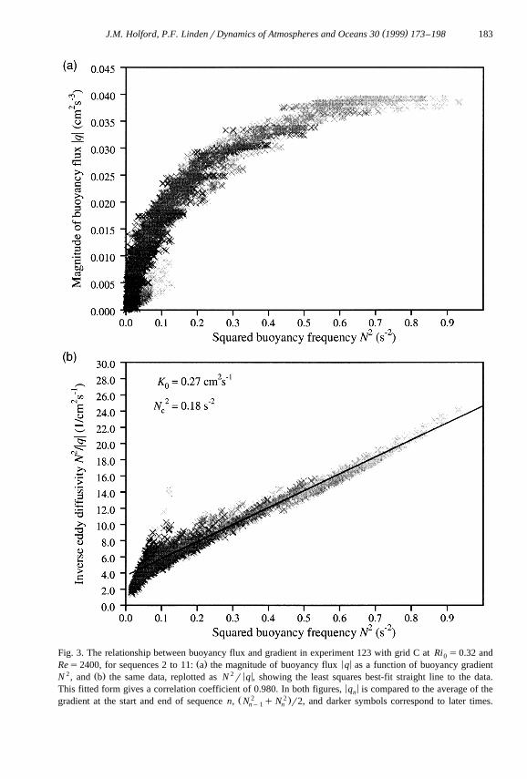
Density profiles are measured and processed as described in Section 2, to giveprofiles of N and q. Fig. 3a shows the relationship between q and N 2 for theexperiment shown in Fig. 1. All data from the discretised 0.1 cm profiles and alltimesteps nG2 are plotted on this figure, and increasing greyscale intensity correspondsto increasing time. These data collapse very well, showing that q is a well-definedfunction of N 2, despite the presence of the upper and lower boundaries of the tankwhich will modify the turbulence field locally.

By extension of the diffusion of a passive scalar in an unstratified fluid, we assume arelationship of the form:

qsyK N 2 N 2 , 3.1Ž . Ž .b


Fig. 3. The relationship between buoyancy flux and gradient in experiment 123 with grid C at Ri s0.32 and0Ž . < <Res2400, for sequences 2 to 11: a the magnitude of buoyancy flux q as a function of buoyancy gradient

2 Ž . 2 < <N , and b the same data, replotted as N r q , showing the least squares best-fit straight line to the data.< <This fitted form gives a correlation coefficient of 0.980. In both figures, q is compared to the average of then

Ž 2 2 .gradient at the start and end of sequence n, N q N r2, and darker symbols correspond to later times.ny 1 n


where K is the eddy diffusivity. In order to find K , we plot yN 2rq s1rK againstb b b

N 2, as shown in Fig. 3b. A straight line least squares fit to these data show that K isb

reasonably approximated by:

K0K s . 3.2Ž .b 2 21qN rNŽ .c

For weak stratifications, the eddy diffusivity is a constant K sK , whereas forb 0

stratifications N 2 RN 2, the diffusivity is significantly reduced below this level. In thec

limit N 24N 2, the buoyancy flux asymptotes to a constant value qsyK N 2.c 0 c

Ž .However, as will be seen in Section 4, Eq. 3.1 is not valid at high Ri. We mayŽ .compare Eq. 3.2 to the parametrisation chosen in the theoretical model of Noh and

Ž .Fernando 1995 :

e1r2 l01r2K se l s , 3.3Ž .b mix 2 2(1qcN l re0

where e is the TKE, l is the mixing length, l is the turbulent integral scale in anmix 0Ž .unstratified fluid, and c is a constant. Our empirical expression, Eq. 3.2 , parametrises

both the effect of a reduced mixing length, and of a reduction in TKE, as Ri increases.

Fig. 4. Values of the eddy diffusivity K in the limit of zero stratification, as a function of U M. Results from0 0

grids A, C and D are shown, with the symbols listed in Table 1, and the least squares best-fit linearrelationship.


Ž . Ž . 1r2As Ri™0, Eq. 3.2 gives K sK while Eq. 3.3 gives K se l , so the twob 0 b 0 0

parametrisations are equivalent and represent a constant eddy diffusivity. As Ri™`,Ž . 2 2 2 Ž .Eq. 3.2 gives K sK N rN and hence qsyK N , while Eq. 3.3 givesb 0 c 0 c

K se rc1r2N and hence qsye Nrc1r2, so the two parametrisations are equivalentb ` `

only if e sc1r2K N 2rN.` 0 c

It is expected that K and N 2 depend on the characteristics of the turbulence, and0 c

therefore on the external scales U, d and M. Data were taken from 11 experiments inthe range Ri Q1.5, and the eddy diffusivity calculated from each. The coefficient K0 0

was found to depend on the mesh length M, as well as the velocity scale U , as shown0

in Fig. 4. For all experiments, K s6.7=10y3U M.0 0

The critical stratification N 2 at which buoyancy effects become important can bec

expressed in terms of a critical Ri, Ri sN 2L2 rU 2, so that:c c 0 0

K0K s . 3.4Ž .b 1qRirRiŽ .c

For experiments with grids C and D, Ri s0.065. However, for experiments with thec

grid A, the smallest grid, and consequently the lowest Re, stratification affected the flowat a lower Ri s0.01. At these low Re, turbulence develops in the wake of the rakec

from 3D instabilities of the Karman vortex street, whereas at higher Re, the Karman´ ´ ´ ´vortices are turbulent on formation. The differences in the value of Ri suggest that thec

Ž .Fig. 5. Evolution of the mixing efficiency h with Ri , for experiment 123 Ri s0.32 and Res2400 ,b 0Ž 1r2 .showing the extrapolation based on an empirical functional form hs aRi q bRi back to a value of0 0

h s0.039 at Ri s0.32.0 0


Ž .Fig. 6. The evolution of experiment 125 with grid C at Ri s1.72, Res1050: a the sequence of density0Ž . y3 Ž .profiles, r z , each subsequent profile shifted by 0.004 g cm , and b the sequence of buoyancy frequencyn2Ž . y2profiles, N z , each subsequent profile shifted by 2.0 s , for ns0,2, . . . ,24.n


effect of stratification is more significant in suppressing the 3D instabilities at low Rethan in damping existing turbulence structures at higher Re. With grid A, previouslyunobserved layering behaviour occurred for 0.1QRi Q1.5, which is discussed in0

Ž .Holford and Linden 1999b . For Ri R1.5, the evolution of the flow with grid A was0Ž .investigated by Holford and Linden 1999a , and will be discussed in Section 4.

3.2. Global behaÕiour

The mixing efficiency h decreases in all experiments almost linearly with time.Ž .Alternatively, the evolution of the experiment can be followed on a plot of h t against

Ž . Ž .the Ri t , as shown in Fig. 5. As the experiment progresses, both Ri t ™0 andb bŽ .h t ™0 as t™`. As the well-mixed boundary layers grow, a greater fraction of the

fluid depth is only weakly stratified. Since the buoyancy flux q is an increasing functionof N 2, the boundary layers support a smaller flux than the stratified interior. Hence the

Ž .depth-averaged buoyancy flux and, from Eq. 2.7 , h decrease as the boundary layersgrow.

4. Evolution of the buoyancy field at high Ri

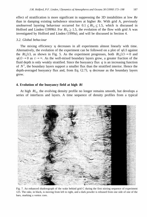
At high Ri , the evolving density profile no longer remains smooth, but develops a0

series of interfaces and layers. A time sequence of density profiles from a typical

Fig. 7. An enhanced shadowgraph of the wake behind grid C during the first stirring sequence of experiment125. The rake, in black, is moving from left to right, and a dark powder is released from one side of one of thebars, marking a vortex core.


layering experiment with grid C is shown in Fig. 6a, and the associated buoyancyfrequency profiles are shown in Fig. 6b. The layering develops across the whole tankdepth at the same rate, and with a regular vertical scale.

Ž .Layering at this Ri with grid A was investigated by Holford and Linden 1999a , as0

discussed in the introduction. The important result of this work is that similar dynamicsis observed at these high Ri , even with grid configurations for which Re is much0

higher. Fig. 7 is a shadowgraph of the wake behind grid C, at Res1050, with a powderdye streak marking a distorted vortex core. Even with grid F, at the largest Res3300, astreak of dye shed from a bar during layering remained coherent, and developed thesame form of vertical perturbations. A vortex street pattern is observed behind a circular

5 Ž Ž ..cylinder up to Re f3=10 Tritton 1988 , although for Re R400 the vortices ared d

turbulent at their formation. Our observations show that stratification maintains thisvortical component of the flow, and damps turbulent motions, so the vertical vorticitydominates the evolution at early times.

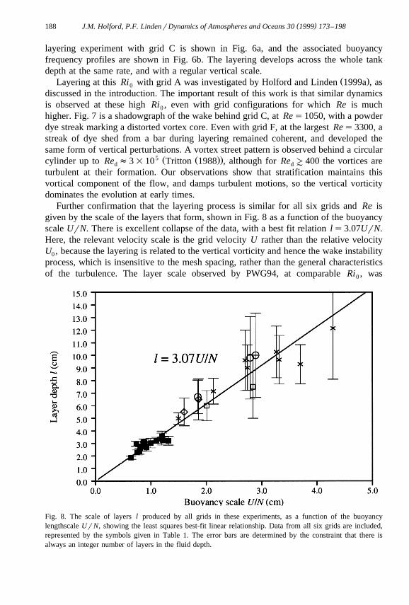
Further confirmation that the layering process is similar for all six grids and Re isgiven by the scale of the layers that form, shown in Fig. 8 as a function of the buoyancyscale UrN. There is excellent collapse of the data, with a best fit relation ls3.07UrN.Here, the relevant velocity scale is the grid velocity U rather than the relative velocityU , because the layering is related to the vertical vorticity and hence the wake instability0

process, which is insensitive to the mesh spacing, rather than the general characteristicsof the turbulence. The layer scale observed by PWG94, at comparable Ri , was0

Fig. 8. The scale of layers l produced by all grids in these experiments, as a function of the buoyancylengthscale UrN, showing the least squares best-fit linear relationship. Data from all six grids are included,represented by the symbols given in Table 1. The error bars are determined by the constraint that there isalways an integer number of layers in the fluid depth.


ls2.6UrNq1.0 cm, and the similarity of scale suggests that the same generationmechanism may be responsible. It is clear that, as in previous layering experiments, thelayer thickness is much larger than the buoyancy scale L swrN, where w is theb

vertical turbulent velocity scale, which is significantly less that UrN. L is a measure ofbŽ .the maximum vertical turbulent lengthscale in a stratified fluid Britter et al., 1983 .

Returning to Fig. 6, it can be seen that the positions of interfaces do not alterŽ .significantly with time, even from the early stage of sequence 2 marked A . By

Ž .sequence 6 B , five interfaces are present with an approximately equal buoyancy jumpacross each. The outer interfaces quickly decay, leaving three interfaces; then the central

Ž .interface begins to decay, and at the end of the experiment C the fluid is approaching athree-layer structure. The positions of decaying interfaces are marked by D. Theprocesses of layer development and decay are discussed further in Section 4.1.

4.1. Local behaÕiour

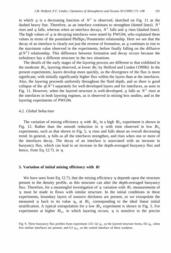
Profiles of q calculated for a high Ri experiment, corresponding to the threen 0

sequences ns2, 6 and 24 are shown in Fig. 9a, b and c. During sequence 2, q takes2

very low values at the positions of the developing interfaces. There are large divergencesof flux, indicative of the developing structure, as the fluid is mixed up within each layer.By the end of sequence 6, q is more uniform in the interior, and decreases linearly to6

< <zero in the well-mixed boundary layers. The uniformity of q shows that the fluid is, atthis time, in a quasi-steady state. The subsequent decay of interfaces is not quasi-steady,and the decaying central interface in sequence 24 is marked by a local maximum of< <q .24

Fig. 10 shows the relationship between q and N 2 at the beginning and end of theŽ 2 .experiment, at sequences ns2 and 24. There is now no direct q N relationship

equivalent to that in Fig. 3 at low Ri , and the overall patterns are qualitatively different0

between the two times.Insight into the layer development is gained by identifying the layers and interfaces in

each profile, by the minima and maxima of N 2, respectively, and following thebuoyancy flux at these points alone, as in Fig. 11. On this figure, the broken line stylescorresponds to an interface, while the solid linestyles corresponds to layers. Fig. 11adisplays the whole range of behaviour, and Fig. 11b is an enlargement of the weaklystratified range. Initially, the buoyancy frequency is everywhere approximately theinitial value, N 2 s0.74 sy2 . However, as discussed in Section 2.2, the density profileextrapolation to the boundaries is relatively unsuccessful for the initial profile, andconsistent flux measurements can only be calculated from the second stirring sequence,by which time the interfaces have N 2 f1.6 sy2 and the layers have N 2 f0.5 sy2 . Thebuoyancy flux is larger at the positions where the layers are developing than at theinterfaces. This divergence of buoyancy flux leads to the development of a stronglayered structure.

Within the layers, N 2 decreases monotonically with time, and q first increases andŽ 2 .then rapidly falls in the manner of the weakly stratified q N relationship discussed in

Section 3.1, shown in Fig. 11 as the solid heavy line. At the developing interfaces, N 2

increases and q also increases. Then, once each interface is well-defined, a relationship


in which q is a decreasing function of N 2 is observed, sketched on Fig. 11 as theŽ . 2dashed heavy line. Therefore, as an interface continues to strengthen dotted lines , N

2 Ž .rises and q falls, whereas when an interface decays, N falls and q rises dashed lines .The high values of q at decaying interfaces were noted by PWG94, who explained thesevalues in terms of the postulated PhillipsrPosmentier relationship. Here we see that thedecay of an interface is clearly not just the reverse of formation, as q continues to rise tothe maximum value observed in the experiments, before finally falling on the diffusiveŽ 2 .q N relationship. This difference between formation and decay occurs because the

turbulence has a different structure in the two situations.The details of the early stages of the layering process are different to that exhibited in

Ž .the moderate Ri layering observed, at lower Re, by Holford and Linden 1999b . In the0

present experiments, layers develop more quickly, as the divergence of the flux is moresignificant, with initially significantly higher flux within the layers than at the interfaces.Also, the layering proceeds uniformly throughout the fluid depth, and so there is good

Ž 2 .collapse of the q N separately for well-developed layers and for interfaces, as seen inFig. 11. However, when the layered structure is well-developed, q falls as N 2 rises atthe interfaces in both layering regimes, as is observed in mixing box studies, and in thelayering experiments of PWG94.

4.2. Global behaÕiour

The variation of mixing efficiency h with Ri in a high Ri experiment is shown inb 0

Fig. 12. Rather than the smooth reduction in h with time observed in low Ri0

experiments, such as that shown in Fig. 5, h rises and falls about an overall decreasingtrend. In general, h falls as all the interfaces strengthen, and rises when one or more ofthe interfaces decay. The decay of an interface is associated with an increase inbuoyancy flux, which can lead to an increase in the depth-averaged buoyancy flux and

Ž .hence, from Eq. 2.7 , in h.

5. Variation of initial mixing efficiency with Ri

Ž .We have seen from Eq. 2.7 , that the mixing efficiency h depends upon the structurepresent in the density profile, as this structure can alter the depth-averaged buoyancyflux. Therefore, for a meaningful investigation of h variation with Ri, measurements ofh must be made in flows with similar structure. In the initial conditions in theseexperiments, boundary layers of nonzero thickness are present, so we extrapolate themeasured h back to its value h at Ri corresponding to the ideal linear initial0 0

stratification. A typical extrapolation for a low Ri experiment is shown in Fig. 5. For0

experiments at higher Ri , in which layering occurs, h is sensitive to the precise0

Ž . Ž .Fig. 9. Three buoyancy flux profiles from experiment 125: a q , as the layered structure forms, b q , when2 6Ž .five similar interfaces are present, and c q , as the central interface of three weakens.24


< < 2Fig. 10. The relationship between the magnitude of buoyancy flux q and buoyancy gradient N inŽ . Ž .experiment 125 at two stages: a ns2 as the layered structure forms, and b ns24, when three interfaces

< < Ž 2 2 .are present. Again, q is shown as a function of N q N r2.n ny1 n


< < 2 Ž 2Fig. 11. The relationship between buoyancy flux q and buoyancy gradient N in experiment 125 N s0.740y2 . Ž .s at selected vertical positions, during the entire experiment. Four layers solid lines and five interfacesŽ .dotted lines while strengthening, dashed lines while decaying are shown, and the arrows indicate time

Ž . Ž . 2 y2evolution. a shows the whole range of behaviour, and b is an enlargement of N -1 s , to show moredetail in this range. The heavy solid line is diffusive behaviour predicted from the lower Ri experiments, and0

the heavy dashed line is a sketch of the behaviour of well-developed interfaces.


Ž .Fig. 12. Evolution of the mixing efficiency h with Ri , for experiment 125. Here the average value solid lineb

is used to estimate h s0.024 at Ri s1.72.0 0

dynamics of the interfaces, and a time average value for h is taken, as shown in Fig.0

12.The resulting h from experiments using grids A, C and D are plotted against Ri in0 0

Fig. 13. For Ri Q1.5, when layering does not occur, the scaling used collapses the data0

for h with grids C and D onto an increasing curve. For grid A, values for h at0 0

Ri Q0.3 follow the same scaling, but above this threshold, layers develop by a separate0

mechanism, as discussed in Section 3.1, and as a result h is lower. For Ri R1.5, in the0 0

layering regime, h decreases for grids C and D as Ri increases, but falls more rapidly0

for grid C, which has the higher solidity. The more solid grid generates more vorticesper unit area, and so requires a different scaling in the high Ri regime. These0

experiments demonstrate a maximum in h at a critical Ri , as observed in the0 0Ž .experiments on mixing across interfaces by Linden 1980 .

The maximum value of the h measured is around 0.05, which is comparable with0Ž .values from some other experiments, including Huq and Britter 1995 and PWG94.

These values are low compared to values for the maximum flux Richardson number,ŽRff0.15–0.25 in shear-driven mixing suggested by turbulence closure theories e.g.,

. Ž .Ellison, 1957 , by oceanographic measurements e.g., Peters and Greggs, 1988 , and byŽ .laboratory experiments e.g., Rohr et al., 1984 . It is possible that the observed low

values of h, which is proportional to the spatial average of q, reflect the spatial andtemporal intermittency of regions of the peak q. In addition, the ratio of q to viscousdissipation, which is represented by Rf , may be sensitive to the nature of the mixing


Fig. 13. The variation in mixing efficiency h at the ideal initial Ri, Ri for experiments with grids A, C and0 0

D, displayed using the symbols from Table 1, showing the peak at the boundary between layering andnonlayering regimes for grids C and D. In experiments with grid A at Ri )0.8, h was too small to be0 0

resolved with the current measuring system.

process, resulting in a lower value of Rf for this mechanical mixing than for theshear-driven mixing.

6. Conclusions

The primary conclusion of this work is that the layering observed is not a result of thePhillipsrPosmentier mechanism. At high values of the overall Ri, Ri , the regions of0

vertical vorticity dominate the flow evolution, and cause the formation of a layeredstructure in the density profile through an interaction between the vortices and stratifica-tion. The ubiquity of this dynamical behaviour for several grid geometries, and over awide range of 500-Re-4000, has been shown, with a well-defined layer scale ofls3.07UrN.

In low Ri flows, we have measured a Ri-dependent eddy diffusivity which0

represents the relationship between buoyancy flux q and local Ri. In the limit asRi™0, the eddy diffusivity approaches a constant value of K s6.7=10y3U M. The0 0

Ri at which the stratification first begins to affect the flow is a constant for larger grids,Ž .Ri f0.065, and the reduction in the eddy diffusivity is given by Eq. 3.4 .c

The buoyancy flux profiles taken in high Ri layered flows show that at fully0

developed and decaying the interfaces, the flux is governed by a relationship similar to


that observed in mixing box experiments, in that the flux decreases with increasingbuoyancy gradient. Within the layers, the flux approaches the value given by thediffusive relationship measured in low Ri flows. In contrast, where the vortex cores0

remain vertical and the layers first develop, the flux is less than predicted by either thelayer or interface relationships. Although there is a well-defined relationship betweenbuoyancy flux and gradient once the layered structure is formed, this is not the caseduring the development of layers, which cannot therefore be a result of the PhillipsrPos-mentier instability.

Ž . Ž 2 .The model of Balmforth et al. 1997 predicts an N-shaped q N relationship at theŽ 2 .equilibrium TKE distribution. In the initial stages of the present experiments, the q N

relationship takes approximately this form, see Fig. 11, but it is not an equilibriumrelationship and, as the interfaces sharpen, q decreases with further increases in N 2.

Ž 2 .Once the layered structure has developed there is a well-defined q N relationship witha maximum in that experiment at N 2 f1 sy2 . This relationship is of the form assumedin the PhillipsrPosmentier model, but does not hold in our experiments in the initial

Ž 2 .stages when there is less structure in the profile. Hence, we see that the peaked q Nrelationship is a result of the layering, rather than an explanation for its development.

For all but the lowest Re flows, the initial mixing efficiency is shown to reach amaximum value of h f0.05 at Ri f1.5, which corresponds to the boundary between0 0

diffusive and layering behaviour. Below this critical Ri , the mixing efficiency is0

independent of grid geometry, whereas at larger Ri , it varies with the grid solidity. As0

the layered structure develops, the mixing efficiency reduces still further, althoughdecaying interfaces can lead to an increase in mixing efficiency. Therefore, we see thatthe structure of the stratification, as well as an overall Ri, affects the amount of mixing,as measured by the mixing efficiency.

Although these experiments use a specialised stirring mechanism, we believe that thecontrol of local mixing by the pattern of vertical vorticity may be important in manyhigh Ri flows, where this vorticity component is a dominant feature. Oceanographic andatmospheric motions show that much of the kinetic energy resides in mesoscale eddieswhich are characterised by large values of the vertical vorticity. As eddies ‘slide’ over

Ž Ž ..one another dissipation occurs see Fincham et al. 1994 . Also vortex lines are tilted asin these experiments. Our results suggest this may be a mechanism that leads to layerformation.

We have also shown that in these experiments, the variation of mixing efficiencywith an overall Ri has no simple relation to the local fluxrgradient relationship when0

the structure of the flow is evolving and changing. Therefore, observational measure-ments of buoyancy flux averaged over regions of evolving structure may give complexresults. Parametrisations may need to take account of the evolution of the local profile aswell as instantaneous gradients.

Acknowledgements

The authors would like to thank all those at the Environmental Flow ResearchLaboratory, at the University of Surrey, and especially the technician Mr. Tom Lawton,


for their support of this project. In addition, we would like to thank the technical staffMr. David Page-Croft, Mr. Brian Dean, Mr. David Lipman and Mr. Caspar Williams forassistance with the laboratory work at DAMTP. This work was supported by the NERCunder research grant GR3r8891.

References

Balmforth, N.J., Llewellyn Smith, S.G., Young, W.R., 1997. Dynamics of interfaces and layers in a stratifiedturbulent fluid. J. Fluid Mech. 355, 329–358.

Barenblatt, G.I., Bertsch, M., Dal Passo, R., Prostokishin, V.M., Ughi, K., 1993. A mathematical model ofturbulent heat and mass transfer in stably stratified shear flow. J. Fluid Mech. 253, 341–358.

Batchelor, G.K., 1949. Diffusion in a field of homogeneous turbulence: I. Eulerian analysis. Aust. J. Sci. Res.2, 437–450.

Britter, R.E., Hunt, J.C.R., Marsh, G.L., Snyder, W.H., 1983. The effects of stable stratification on turbulentdiffusion and the decay of grid turbulence. J. Fluid Mech. 127, 27–44.

Dalaudier, F., Sidi, C., Crochet, M., Vernin, J., 1994. Direct evidence of ‘sheets’ in the atmospherictemperature field. J. Atmos. Sci. 51, 237–248.

Davis, R.W., Moore, E.F., 1982. A numerical study of vortex shedding from rectangles. J. Fluid Mech. 116,475–506.

Ellison, T.H., 1957. Turbulent transport of heat and momentum from an infinite rough plane. J. Fluid Mech. 2,456–466.

Fernando, H.J.S., 1991. Turbulent mixing in stratified fluids. Annu. Rev. Fluid Mech. 23, 455–493.Fincham, A.M., Maxworthy, T., Spedding, G.R., 1994. Energy dissipation and vortex structure in freely

decaying, stratified grid turbulence. Dyn. Atmos. Oceans 23, 155–169.Holford, J.M., Linden, P.F., 1999a. The development of layers in a stratified fluid. Mixing and Dispersion in

Stably Stratified Flows. Proc. of 5th IMA Conf. on Stratified Flows. Oxford Univ. Press, pp. 165–179.Holford, J.M., Linden, P.F., 1999b. Boundary-driven layering in a turbulent stratified flow. Phys. Fluids,

submitted.Huq, P., Britter, R.E., 1995. Turbulence evolution and mixing in a two-layer stably stratified fluid. J. Fluid

Mech. 285, 41–67.Linden, P.F., 1979. Mixing in stratified fluids. Geophys. Astrophys. Fluid Dyn. 13, 3–23.Linden, P.F., 1980. Mixing across a density interface produced by grid turbulence. J. Fluid Mech. 100,

691–703.Liu, H.-T., 1995. Energetics of grid turbulence in a stably stratified fluid. J. Fluid Mech. 296, 127–157.Majda, A.J., Grote, M.J., 1997. Model dynamics and vertical collapse in decaying strongly stratified flows.

Phys. Fluids 9, 2932–2940.Miyazaki, T., Fukumoto, Y., 1992. Three-dimensional instability of strained vortices in a stably stratified fluid.

Phys. Fluids A 4, 2515–2522.Noh, Y., Fernando, H.J.S., 1995. Onset of stratification in a mixed layer subjected to a stabilizing buoyancy

flux. J. Fluid Mech. 304, 27–46.Park, Y.-G., Whitehead, J.A., Gnanadesikan, A., 1994. Turbulent mixing in stratified fluids: layer formation

and energetics. J. Fluid Mech. 279, 279–311.Peters, H., Greggs, M.C., 1988. On the parametrization of equatorial turbulence. J. Geophys. Res. 93,

1199–1218.Phillips, O.M., 1972. Turbulence in a strongly stratified fluid — is it unstable?. Deep-Sea Res. 19, 79–81.Posmentier, E.S., 1977. The generation of salinity finestructure by vertical diffusion. J. Phys. Oceanogr. 7,

298–300.Rohr, J.J., Itsweire, E.C., van Atta, C.W., 1984. Mixing efficiency in stably stratified decaying turbulence.

Geophys. Astrophys. Fluid Dyn. 29, 221–236.Ruddick, B.R., McDougall, T.J., Turner, J.S., 1989. The formation of layers in a uniformly stirred density

gradient. Deep-Sea Res. 36, 597–609.


Stansby, P.K., Slaouti, A., 1993. Simulation of vortex shedding including blockage by the random-vortex andother methods. Int. J. Numer. Methods Fluids 17, 1003–1013.

Stillinger, D.C., Helland, K.N., van Atta, C.W., 1983. Experiments on the transition of homogeneousturbulence to internal waves in a stratified fluid. J. Fluid Mech. 131, 91–122.

Taylor, G.I., 1915. Eddy motion in the atmosphere. Philos. Trans. R. Soc. London 215A, 1–26.Tritton, D.J., 1988. Physical Fluid Dynamics. Oxford Science Publications, 519 pp.Turner, J.S., 1968. The influence of molecular diffusivity on turbulent entrainment across a density interface.

J. Fluid Mech. 33, 639–656.Turner, J.S., 1973. Buoyancy Effects in Fluids. Cambridge Univ. Press, 367 pp.Winters, K.B., Lombard, P.N., Riley, J.J., D’Asaro, E.A., 1995. Available potential energy and mixing in

density-stratified fluids. J. Fluid Mech. 289, 115–128.

turbulent mixing in a stratified fluidmaecourses.ucsd.edu/groups/linden/pdf_files/74hl99.pdf ·...

Documents