on the properties of beta-gamma distribution · on the properties of beta-gamma distribution 188...

Journal of Modern Applied StatisticalMethods

Volume 6 | Issue 1 Article 18

5-1-2007

On the Properties of Beta-Gamma DistributionLingji KongUnion College

Carl LeeCentral Michigan University

J.H. SepanskiCentral Michigan University

Follow this and additional works at: http://digitalcommons.wayne.edu/jmasm

Part of the Applied Statistics Commons, Social and Behavioral Sciences Commons, and theStatistical Theory Commons

This Regular Article is brought to you for free and open access by the Open Access Journals at DigitalCommons@WayneState. It has been accepted forinclusion in Journal of Modern Applied Statistical Methods by an authorized editor of DigitalCommons@WayneState.

Recommended CitationKong, Lingji; Lee, Carl; and Sepanski, J.H. (2007) "On the Properties of Beta-Gamma Distribution," Journal of Modern AppliedStatistical Methods: Vol. 6 : Iss. 1 , Article 18.DOI: 10.22237/jmasm/1177993020Available at: http://digitalcommons.wayne.edu/jmasm/vol6/iss1/18

http://digitalcommons.wayne.edu/?utm_source=digitalcommons.wayne.edu%2Fjmasm%2Fvol6%2Fiss1%2F18&utm_medium=PDF&utm_campaign=PDFCoverPages

http://digitalcommons.wayne.edu/?utm_source=digitalcommons.wayne.edu%2Fjmasm%2Fvol6%2Fiss1%2F18&utm_medium=PDF&utm_campaign=PDFCoverPages

http://digitalcommons.wayne.edu/jmasm?utm_source=digitalcommons.wayne.edu%2Fjmasm%2Fvol6%2Fiss1%2F18&utm_medium=PDF&utm_campaign=PDFCoverPages


http://digitalcommons.wayne.edu/jmasm/vol6?utm_source=digitalcommons.wayne.edu%2Fjmasm%2Fvol6%2Fiss1%2F18&utm_medium=PDF&utm_campaign=PDFCoverPages

http://digitalcommons.wayne.edu/jmasm/vol6/iss1?utm_source=digitalcommons.wayne.edu%2Fjmasm%2Fvol6%2Fiss1%2F18&utm_medium=PDF&utm_campaign=PDFCoverPages

http://digitalcommons.wayne.edu/jmasm/vol6/iss1/18?utm_source=digitalcommons.wayne.edu%2Fjmasm%2Fvol6%2Fiss1%2F18&utm_medium=PDF&utm_campaign=PDFCoverPages


http://network.bepress.com/hgg/discipline/209?utm_source=digitalcommons.wayne.edu%2Fjmasm%2Fvol6%2Fiss1%2F18&utm_medium=PDF&utm_campaign=PDFCoverPages



http://digitalcommons.wayne.edu/jmasm/vol6/iss1/18?utm_source=digitalcommons.wayne.edu%2Fjmasm%2Fvol6%2Fiss1%2F18&utm_medium=PDF&utm_campaign=PDFCoverPages

Journal of Modern Applied Statistical Methods Copyright © 2007 JMASM, Inc. May, 2007, Vol. 6, No. 1, 187-211 1538 – 9472/07/$95.00

187

On the Properties of Beta-Gamma Distribution

Lingji Kong Carl Lee J. H. Sepanski Union College Central Michigan University

A class of generalized gamma distribution called the beta-gamma distribution is proposed. Some of its properties are examined. Its shape can be reversed J-shaped, unimodal, or bimodal. Reliability and hazard functions are also derived, and applications are discussed. Key words: Gamma distribution, Beta distribution, reliability function, hazard function, MLE, application.

Introduction

Let ( )f ⋅ and ( )F ⋅ be the probability density function and the cumulative distribution function (cdf) of a random variable, respectively. Eugene, Lee, and Famoye (2002) first introduced a generalized distribution based on the logit of the beta random variable with a cumulative distribution function given by

=)(xG ∫ −− −)(

0

11 ,)1(),(

1 xF

dtttB

βα

βα∞<< βα,0 ,

and the corresponding probability density function is

[ ] ),()(1)(),(

1)( 11 xfxFxFB

xg −− −= βα

βα∞<< βα,0

Lingji Kong is an Assistant Professor of Mathematics. His email is [email protected]. Carl Lee is Professor of Statistics and senior research fellow at the Center for Applied Research and Technology, Central Michigan University. His research area is in generalized distributions and data mining. His email is [email protected]. Jungsywan Sepanski is an Associate Professor of Statistics in the Mathematics Department at Central Michigan University. Her research area is in measurement error and estimation. Her email is [email protected].

Eugene, et al. (2002) studied properties of

( )g x when ( )F ⋅ is the cdf of a normal distribution. Maynard (2003) examined the case when ( )F ⋅ is the cdf of an exponential distribution.

Gamma distribution and its generalized distributions (e.g. McDonald, 1984) have been applied widely to the analyses of income distributions, life testing, and many physical and economical phenomena (e.g. Farewell, 1977, Lawless, 1980). In this article, the case when

( )F ⋅ is the cdf of the gamma distribution is studied.

A random variable X is said to have a beta-gamma distribution, ),,,( λρβαBG , if its probability density function is given by

[ ] ,)(1)()(),(

)( 11/1

−−−−

−Γ

= βαρ

λρ

λρβαxFxF

Bexxg

x

∞<< λρβα ,,,0 , 0>x , (1) where F(x) is the cdf of the gamma distribution with parameters ρ and λ . One can also introduce a location parameter ξ in the density in (1) by replacing x with ξ−x where

.∞<<∞− ξ In the rest of this article, it is assumed that ξ is zero. When both α and β are integers with βα + being a bounded integer, the beta-gamma density function in (1) is the marginal probability density function of

ON THE PROPERTIES OF BETA-GAMMA DISTRIBUTION

188

the thα order statistic in a random sample of size βα + from the gamma distribution with

parameters ρ and λ . When ,1== βα the beta-gamma distribution yields the gamma distribution. When ,1=ρ the beta-gamma distribution is beta-exponential distribution introduced in Maynard (2003).

Properties

The limit of ( )g x as x goes to 0 and the mode of the probability density function ( )g x in (1) is given in Lemma 1. The modes for cases when 1≤ρα and 1>ρα are studied respectively. Although some cases can be shown mathematically, plotting the function g(x) using Maple computer programs are employed to examine shapes and modalities for other cases. Illustrative graphs of ( )g x based on observations from numerous plots are presented. Numerical percentiles are presented in Table 7 to Table 9. Limits

Lemma 1: The limit as x goes to 0 of the beta-gamma probability density function ( )g x in (1) is

=→ )(lim 0 xgx

1

if 11 if 1

( ) ( , )0 if 1

Bα α

αρ

αρρ α β ρ λ

αρ

−

⎧∞ <⎪⎪ =⎨Γ⎪⎪ >⎩

(2) The proof is given in Appendix. Modes of ( )g x When 1≤αρ

Note that the derivative xxfdxdf /)/1(/ λρ −−= . The first

derivative of the logarithm of the probability density function g(x) is given by

fF

fFx

x−−+−+−−

111/1 βαλρ

. (3) (2.3)

The mode(s) mx of )(xg if exists is the solution to the equation by setting (3) to be zero.

It is shown below that g (x) has a reversed-J shape when 1≤ρα and 1≥β . The derivative in (3) is equal to

[ ]f 1(1 ) ( 1)xf ( 1 x / )F1 F xF

− β + α − + ρ − − λ−

.

(4) When 1≥β , the first term in (4) is less or equal to 0. Also,

d [( 1)xf ( 1 x / )F]dx

1 x /( 1)f ( 1)xfx

F / ( 1 x / )f( 1)f xf / F /

α − + ρ − − λ

ρ − − λ= α − + α −

− λ + ρ − − λ= αρ − − α λ − λ

which is negative when 1≤αρ . This implies that Fxxf )/1()1( λρα −−+− is a decreasing function. Because

0)/1()1( =−−+− Fxxf λρα when 0=x , the second term in (4) is therefore negative. That is, )(' xg is negative. By (2) and the fact that

)(lim xgx ∞→ =0, )(xg has a reversed-J shape for the cases when 1≤ρα and 1≥β with maximum occurring at 0=x .

When 1≤α and 1≤ρ regardless of β, one can see that )(xg has a reversed-J shape by rewriting )(xg as

[ ]βα

βα)(1)(

)(1)(

),(1)( 1 xFxF

xFxf

Bxg −

−= − .

Because the cdf F is an increasing function and the hazard function )1/( Ff − of the gamma distribution function is a decreasing function when 1≤ρ , )(xg is therefore a decreasing function with ∞=→ )(lim 0 xgx when 1≤α and 1≤ρ .

KONG, LEE, & SEPANSKI 189

Next, graphical results are shown to

examine the cases when 1<β and 1≤αρ with α or ρ greater than 1. Figure 1 represents

cases when 1=αρ . Figure 2 contains cases when 1<αρ . Note that a =α , b = β , and p = ρ in all figures in this article.

Figure 1. Plot of the density function g(x) when 1=ρα , and β =0.25, 0.5, 2, 4


190

When 1=ρα and 1≥β , the beta-

gamma distribution appears to have a reversed-J shape. Figure 1 also shows that when 2=α and 5.0=ρ , it has a non-zero mode for β values of 0.25 and 0.5.

When 1<ρα and 1<β , it is found that )(xg is not necessarily a reverse J-shape, it can be bimodal (with one mode at 0). Figure 3 shows two such cases. The top two are for

,25.0=ρ ,9.3=α and 5.0=β ; the bottom

graph is for ,2=ρ ,49.0=α and 01.0=β . Note that the horizontal axis of the first plot ranges from 0 to 0.01 and the one of the second plot ranges from 0.01 to 2. Tables 1 – 4 give the 2nd non-zero mode in addition to the mode at

0=x for some examples when 1<αρ and 1<ρ . The empty cells are cases where

)(xg is reverse J-shaped and the only mode is at 0=x .

Figure 2. Plot of the density function g(x) when 1<ρα , and β =0.25, 0.5, 2, 4


Figure 3. Graphs of )1,,,( ρβαBG


192

Table 1. Nonzero 2nd mode of )1,,,( ρβαBG with .2/1=ρ

=β 0.01 0.1 0.2 0.3 0.4 0.5 0.6 0.7 0.8 0.9 α =1.8 1.04 1.9 1.31 .529 .234 1.95 1.42 .616 .319 .167 .074 1.99 1.50 .678 .374 .219 .013 .071 .035 .012

Table 2(a). Nonzero 2nd mode of )1,,,( ρβαBG with .4/1=ρ

=β 0.01 0.1 0.2 0.3 0.4 0.5 0.6 0.7 0.8 0.9 =α 3.01

3.02 .365 3.1 .571 3.2 .714 3.3 .826 .274 3.4 .923 .382 3.5 1.01 .460 .193 3.6 1.09 .526 .266 .103 3.7 1.16 .585 .323 .173 .064 3.8 1.22 .638 .373 .222 .124 .052 3.9 1.29 .687 .417 .264 .165 .097 .049

Table 2(b). Nonzero 2nd mode of )1,,,( ρβαBG with .4/1=ρ

=β 0.91 0.92 0.93 0.94 0.95 0.96 0.97 0.98 0.99 =α 3.99 .004 .003 .001

3.995 .005 .004 .003 .002 .001

Table 3. Nonzero 2nd mode of )1,,,( ρβαBG with 6/1=ρ =β .01 0.1 0.2 0.3 0.4 0.5 0.6 0.7 0.8 0.9

=α 5.8 1.21 .67 .41 .27 .17 .10 .05 5.9 1.24 .69 .44 .29 .19 .12 .07 .036 .020 5.99 1.27 .72 .48 .31 .21 .14 .09 .052 .026 .008

Table 4. Nonzero 2nd mode of )1,,,( ρβαBG with 2=ρ

β =0.01 0.015 0.1 0.2 0.3 0.4 =α 0.48

0.49 9.85 0.499 9.86 7.656


Note that, for example, when =α 0.48, β =0.01, and 2=ρ , g(x) has an inversed-J shape and therefore does not have a nonzero mode. The range of β where )(xg is bimodal appears to widen as α increases. When bimodality occurs, the nonzero mode increases as the parameter α increases and decreases as the parameter β increases. The bimodality property of beta-gamma distribution is not independent of the gamma parameters ( )ρα , . The bimodality property also exists for beta-normal (Famoye, Lee, & Eugene, 2004). Modes when 1>αρ

The second derivative of the logarithm of )(xg is given by

2 2 2

2 2 2 2

1 x / ( 1)f (1 )f 1 x /x F 1 F x

( 1 x / ) ( 1)f (1 )f 1x F (1 F) x

ρ − − λ α − − β ρ − − λ⎡ ⎤+ +⎢ ⎥−⎣ ⎦⎡ ⎤ρ − − λ α − − β ρ −− + − +⎢ ⎥−⎣ ⎦

. The first term equals to 0 at the mode mx . Hence, when mxx = ,

2

2

2 2

2 2

2

2 2

d ln gdx

( 1 x) ( 1)fx F

( 1)f 1(1 F) x

=

⎡ ⎤ρ − − α −+⎢ ⎥⎢ ⎥−⎢ ⎥β − ρ −+ +⎢ ⎥−⎣ ⎦

.

(5) When ,1,1 ≥≥ αβ and 1≥ρ , (5) is less than 0 at mxx = . In this case, since there must be a minimum between any two maxima and that

)(lim 0 xgx→ =0 and )(lim xgx ∞→ =0, it is concluded that )(xg is unimodal with a concave shape.

When 1≥β and 1>αρ with 1<α or 1<ρ , though not being shown mathematically, graphs of such cases indicate that beta-gamma density function )(xg is also unimodal with a concave shape. Based on numerous graphs, the density functions )(xg is unimodal when 1>αρ regardless the value of β . The following illustrates some examples when 1>αρ .


194

In this case )(xg is unimodal with a

concave shape and the mode is nonzero. Tables 5 and 6 tabulate modes for )1,2,,( βαBG and

)1,2/1,,( βαBG when 1>ρα . The results indicate that

when 1>ρα the mode increases as α increases and that the mode decreases as β increases for both )1,2,,( βαBG and )1,2/1,,( βαBG ; see

also Figure 4. For other cases when ,1>αρ this pattern holds for other values of parameters ρ and λ though the computation results are not reported here. Percentiles of )(xg

The 50th, 75th, 90th, and 95th percentiles of )1,,,( ρβαBG are computed and tabulated in the following Tables 7-9.

Figure 4. Plot of the density function g(x) when 1>ρα , and β =0.5, 1.5


Table 5. Modes for )1,2,,( βαBG when 1>ρα β =0.2 0.5 1 1.5 2 2.5 5 10 α =1 2.236 1.414 1.000 .8165 .7071 .6325 .4472 .3162 α =1.5 3.206 2.162 1.555 1.270 1.097 .9775 .6815 .4744 α =2 3.729 2.628 1.938 1.598 1.386 1.238 .8644 .5994 α =2.5 4.087 2.963 2.229 1.856 1.618 1.451 1.018 .7063 α =5 5.055 3.915 3.111 2.672 2.379 2.163 1.570 1.107 α =10 5.913 4.787 3.964 3.498 3.176 3.947 2.228 1.626

Table 6. Modes for )1,2/1,,( βαBG when 1>ρα .

β =0.2 0.5 1 1.5 2 2.5 5 10 α =2.5 0.832 .3919 .1692 .0903 .0545 .0359 .0291 .0154 α =5 1.788 1.129 .7150 .5137 .3923 .3114 .1337 .0735 α =10 2.653 1.798 1.286 1.016 .8411 .7155 .3925 .1812

Table 7. Percentiles of )1,,,( ρβαBG with 2/1=ρ

α β 50th 75th 90th 95th 0.25 0.25 .2275 2.011 5.260 7.855 0.5 .0235 .4372 1.684 2.846 1 .0031 .0831 .4479 .8765 2 .0005 .0169 .1116 .2445 4 .0001 .0038 .0277 .0654 0.5 0.25 .9346 3.194 6.550 9.171 0.5 .2275 1.054 2.530 3.716

1 .0508 .3014 .8588 1.358 2 .0115 .0802 .2632 .4522 4 .0027 .0207 .0752 .1370 1 0.25 1.735 4.163 7.568 10.21

0.5 .6617 1.735 3.317 4.570 1 .2275 .6617 1.353 1.921

2 .0706 .2275 .5022 .7405 4 .0202 .0706 .1678 .2576 2 0.25 2.473 4.979 8.413 11.06 0.5 1.205 2.405 4.044 5.316

1 .5531 1.123 1.899 2.501 2 .2275 .4817 .8367 1.115

4 .0816 .1824 .3306 .4504 4 0.25 3.160 5.710 9.166 11.82 0.5 1.787 3.057 4.731 6.016

1 .9914 1.649 2.478 3.102 2 .5073 .8444 1.261 1.570

4 .2275 .3872 .5869 .7351


196

Table 8. Percentiles of )1,,,( ρβαBG with 1=ρ

α β 50th 75th 90th 95th 0.25 0.25 .6939 3.106 6.752 9.535 0.5 .1882 1.050 2.710 4.070 1 .0645 .3804 1.067 1.685 2 .0265 .1577 .4517 .7249 4 .0120 .0718 .2065 .3330 0.5 0.25 1.763 4.466 8.125 10.90 0.5 .6925 1.919 3.704 5.077

1 .2877 .8267 1.661 2.328 2 .1285 .3729 .7592 1.075 4 .0512 .1758 .3588 .5086 1 0.25 2.773 5.545 9.210 11.98

0.5 1.386 2.773 4.605 5.991 1 .6931 1.386 2.303 2.996

2 .3466 .6931 1.151 1.498 4 .1733 .3466 .5756 .7489 2 0.25 3.644 6.436 10.10 12.88 0.5 2.115 3.565 5.366 6.720

1 1.228 2.010 2.970 3.676 2 .6931 1.120 1.631 2.000

4 .3766 .6055 .8768 1.071 4 0.25 4.428 7.229 10.90 13.68 0.5 2.836 4.312 6.167 7.556

1 1.838 2.668 3.650 4.363 2 1.159 1.641 2.187 2.571

4 .6931 .9706 1.278 1.490


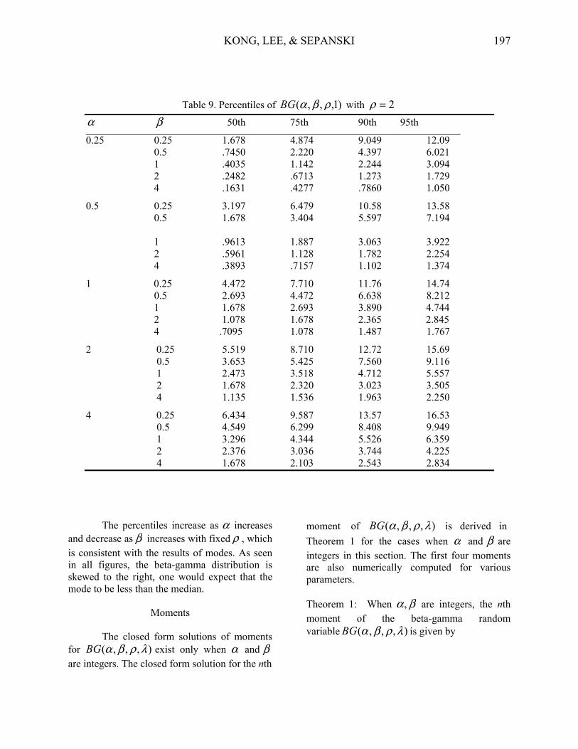
The percentiles increase as α increases and decrease as β increases with fixed ρ , which is consistent with the results of modes. As seen in all figures, the beta-gamma distribution is skewed to the right, one would expect that the mode to be less than the median.

Moments

The closed form solutions of moments for ),,,( λρβαBG exist only when α and β are integers. The closed form solution for the nth

moment of ),,,( λρβαBG is derived in Theorem 1 for the cases when α and β are integers in this section. The first four moments are also numerically computed for various parameters. Theorem 1: When βα , are integers, the nth moment of the beta-gamma random variable ),,,( λρβαBG is given by

Table 9. Percentiles of )1,,,( ρβαBG with 2=ρ

α β 50th 75th 90th 95th 0.25 0.25 1.678 4.874 9.049 12.09 0.5 .7450 2.220 4.397 6.021 1 .4035 1.142 2.244 3.094 2 .2482 .6713 1.273 1.729 4 .1631 .4277 .7860 1.050 0.5 0.25 3.197 6.479 10.58 13.58 0.5 1.678 3.404 5.597 7.194

1 .9613 1.887 3.063 3.922 2 .5961 1.128 1.782 2.254 4 .3893 .7157 1.102 1.374 1 0.25 4.472 7.710 11.76 14.74

0.5 2.693 4.472 6.638 8.212 1 1.678 2.693 3.890 4.744

2 1.078 1.678 2.365 2.845 4 .7095 1.078 1.487 1.767 2 0.25 5.519 8.710 12.72 15.69 0.5 3.653 5.425 7.560 9.116

1 2.473 3.518 4.712 5.557 2 1.678 2.320 3.023 3.505

4 1.135 1.536 1.963 2.250 4 0.25 6.434 9.587 13.57 16.53 0.5 4.549 6.299 8.408 9.949

1 3.296 4.344 5.526 6.359 2 2.376 3.036 3.744 4.225

4 1.678 2.103 2.543 2.834


198

j 11

j kn,k

j 0 k 0

1 j 11 ( 1) ( 1) Ij kB( , )

α+ −β−

= =

⎧β − α + −⎛ ⎞ ⎛ ⎞ ⎫⎪− −⎨ ⎬⎜ ⎟ ⎜ ⎟α β ⎪⎝ ⎠ ⎝ ⎠ ⎭⎩∑ ∑

(6) where

knI , dxFxfx kn∫∞

−=0

)1)(( .

The proof is given in Appendix. The follow Corollary gives E(X) and E(X2) that are used to obtain variance. Corollary 1: When 1,2 == βα and ρ is an

integer, ( )E X and 2( )E X are given by:

)(XE = λρ2 ∑−

=+ −

+−1

0 !)!1(2)!(ρ

ρ ρρλ

ii i

i

= λρ2 ∑−

=+

⎟⎟⎠

⎞⎜⎜⎝

⎛ +

−1

0 2

ρ

ρ

ρρ

ρλi

i

i

;

(7) )( 2XE = ρρλ )1(2 2 +

]2

11

2[)1(1

01

2 ∑−

=++

⎟⎟⎠

⎞⎜⎜⎝

⎛+

++

−+=ρ

ρ

ρρ

λρρi

i

i

(8) The proof is given in Appendix.

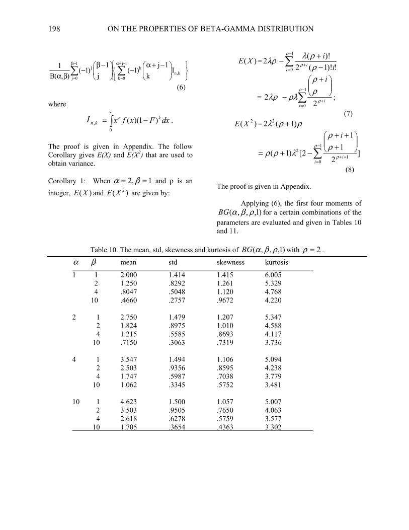
Applying (6), the first four moments of )1,,,( ρβαBG for a certain combinations of the

parameters are evaluated and given in Tables 10 and 11.

Table 10. The mean, std, skewness and kurtosis of )1,,,( ρβαBG with 2=ρ .

α β mean std skewness kurtosis 1 1 2.000 1.414 1.415 6.005 2 1.250 .8292 1.261 5.329 4 .8047 .5048 1.120 4.768 10 .4660 .2757 .9672 4.220 2 1 2.750 1.479 1.207 5.347 2 1.824 .8975 1.010 4.588 4 1.215 .5585 .8693 4.117 10 .7150 .3063 .7319 3.736 4 1 3.547 1.494 1.106 5.094 2 2.503 .9356 .8595 4.238 4 1.747 .5987 .7038 3.779 10 1.062 .3345 .5752 3.481 10 1 4.623 1.500 1.057 5.007 2 3.503 .9505 .7650 4.063 4 2.618 .6278 .5759 3.577 10 1.705 .3654 .4363 3.302 .


Based on the numerical results, the

mean and standard deviation appear to increase with α for a fixed β ; and skewness and kurtosis appear to decrease as α increases for a fixed β in both cases when 2=ρ and

2/1=ρ . Based on Figure 4, the density function has a heavier right tail as α increases. The mean and standard deviation decrease as β decreases for a fixed α . Although the skewness and kurtosis decrease with β when 2=ρ as shown in Table 10, the skewness and kurtosis increase with β when 2/1=ρ and 1≤αρ , as shown in Table 11. However, no clear pattern is noticed when 1>αρ .

Reliability and Hazard Functions

The reliability and hazard functions of

the beta-gamma distribution are derived in this

section. The reliability function, ][1)( xXPxR ≤−= , at time x defined to be

the probability that a unit X survives beyond time x. For a beta-gamma random variable, it is given by

x1 1

0

F(x)1 1

0

11 F (1 F) dF(t)B( , )

11 t (1 t) dtB( , )

α− β−

α− β−

− −α β

= − −α β

∫

∫

where f and F are the density function and cdf of the gamma random variable with parameters ρ and λ , respectively. The hazard function defined to be a instantaneous measure of failure at time x given survival to time x is equal to

Table 11. The mean, std, skewness and kurtosis of )1,,,( ρβαBG with 2/1=ρ

α β mean std skewness kurtosis 1 1 .5000 .7071 2.829 15.00 2 .1814 .2828 3.287 18.66 4 .0604 .1038 3.834 26.22 10 .0124 .0237 4.688 39.71 2 1 .8180 .8468 2.172 10.28 2 .3523 .3830 2.290 11.11 4 .1356 .1586 2.544 13.14 10 .0319 .0413 3.032 17.96 4 1 1.235 .9584 1.762 8.011 2 .6280 .4830 1.669 7.422 4 .2868 .2289 1.718 7.614 10 .0820 .0712 1.955 9.080 10 1 1.900 1.057 1.468 6.683 2 1.154 .5878 1.218 5.491 4 .6508 .3228 1.097 4.941 10 .2505 .1290 1.119 4.968

____________________________________________________________________


200

==)()()(

xRxgxH

∫ −−

−−

−−

−

x

dxxfFFB

xfFFB

0

11

11

)()1(),(

11

)()1(),(

1

βα

βα

βα

βα.

Lemma 2:

(a) )(lim)(lim 00 xgxH xx →→ = (b) λβ /lim =∞→x

The proof is given in Appendix.

The hazard functions of )1,,,( ρβαBG

are plotted. Cases with αρ <1 are presented in Figure 5 and cases with 1≥αρ are given in Figure 6. The graphs in the first column represent the cases αρ =1 with β =1/2, 1, and 2; and those in the second column represent the cases when αρ >1 with β =1/2, 1, and 2 in Figure 6.

Figure 5. Hazard Function of )1,,,( ρβαBG when <αρ 1


Figure 6. Hazard Function of )1,,,( ρβαBG when ≥αρ 1


202

As stated in Lemma 2, the curves of the hazard functions start at the values given in Lemma 1 and go to the value of β as x goes to ∞ regardless the values of other parameters. When 1<αρ and β ≥ 1 (see also Figure 2),

)(xg has a reversed J shape and the trends of hazard functions for β =1 and β =2 (both β >1) are similar (Figure 5). When 1=αρ and β =1/2, the hazard function has a nonzero maximum or minimum. The hazard function is constant when 1=== βρα , sine g(x) is the exponential distribution. Within each plot, a larger α value seems to result in a larger value of the hazard function. When 1>αρ , )(xg has a nonzero mode (see also Figure 4) and the corresponding hazard function is non-decreasing.

When ,1== βα it is Gamma function. λ/1lim =∞→x , which is different from that of

beta-gamma. Also, the hazard function of the beta-gamma can handle bathtub cases where gamma can not. Therefore, the beta-gamma distribution is more flexible. This is especially important when the beta parameter is not near one.

Parameter Estimation Using Maximum Likelihood Method Let nxxx ,......, 21 be a random sample of size n from a beta-gamma distribution defined in (1.1), the log-likelihood function

),,,( λρβαl is then given by

)()()(log

βαβα

ΓΓ+Γn ∑

=

−+n

iixF

1

)(log)1(α

∑=

−−+n

iixF

1))(1log()1(β ∑

=

+n

iixf

1)(log ,

where )(xf and )(xF are the pdf and cdf of the gamma distribution with parameters ρ and

λ , respectively. Let dzzdz /)()( Γ=ψ be the digamma function. The equations for solving the maximum likelihood estimates of ρβα ,, and λ are given in Appendix. The example in the next section, initial estimates of ρ and λ is first computed by assuming the data set follows gamma distribution with 1=α and 1=β , the results from MLE of ( λρ, ) along with 1=α and

1=β then are used as the initial values for solving the equations (A.3) to (A.6).

Applications of the Beta-Gamma Distribution

An application of the proposed distribution is presented using the data sets given in Park, Leslie, and Mertz (1964), Park (1954), Moffa and Costantino (1977). Costantino and Desharnais (1981) established a gamma-state probability distribution for adult numbers in continuously growing populations of the flour beetle Tribolium. The hypothesis that the data set is from a beta-gamma distributed population is tested using the observed frequency distributions of adult numbers for Tribolium castaneum and Tribolium Confusum.

The beta-gamma distribution is fitted to the ten data sets discussed above, and the results are compared to those from gamma distribution and beta-normal distribution proposed by Eugene (2001) where the maximum likelihood method was used. Table 12 tabulates the resulting chi-square values form the goodness-of-fit test for the 10 data sets, and for illustration of the computations Tables 13 and 14 contains results for two of the ten data sets (Data set # 6 and #10). The expected numbers are calculated using the respective distribution with the parameters set at their maximum likelihood estimates. The chi-square goodness-of-fit test is then employed to make a comparison between the observed and expected number of observations under each distribution. Note that a class interval with an expected number less than 5 is combined with the adjacent class to avoid inflating the chi-square test statistic.


It is of no surprise that the proposed beta-gamma distribution fits better than the gamma distribution for all the data sets. Seven of the ten data sets, the beta-gamma distribution fits better than the beta-normal distribution

based on the chi-squares values. Note that, for example, the data set in Table 14 appears to have a long right tail, it is reasonable that beta-gamma distribution performed the best.

Table 12. The resulting 2χ values (p-value, d.f.) from the goodness-of-fit tests for the 10 data sets. Data set Gamma Beta-Normal Beta-Gamma #1 24.03 (0.0043, 9) 5.04 (0.6545, 7) 7.88 (0.3433, 7) #2 48.16 (0, 12) 27.02 (0.0026, 10) 20.50 (0.0249, 10) #3 129.18 (0, 17) 74.85 (0, 15) 72.63 (0, 15) #4 78.07 (0, 11) 25.39 (0.0030, 9) 28.36 (0.0008, 9) #5 23.62 (0.0144, 11) 19.99 (0.0180, 9) 17.89 (0.0365, 9) #6 10.72 (0.3793, 10) 7.42 (0.4913, 8) 7.05 (0.5312, 8) #7 21.67 (0.0169, 10) 10.56 (0.2280, 8) 12.89 (0.1157, 8) #8 55.71 (0, 9) 25.05 (0.0007, 7) 22.28 (0.0023, 7) #9 25.02 (0.2463, 21) 16.85 (0.6001, 19) 16.54 (0.6210, 19) #10 17.19 (0.3076, 15) 17.07 (0.1959, 13) 15.01 (0.3067, 13)


204

Table 13. Observed and Expected Frequencies for Tribolium Confusum Strain # 4(b)

Expected _____________________________________________

valuex − observed Gamma Beta-Normal Beta-Gamma

⎭⎬⎫

5.425.37

⎭⎬⎫

55

10 ⎭⎬⎫

42.636.2

8.78 ⎭⎬⎫

78.785.2

10.63 ⎭⎬⎫

11.801.4

12.12

47.5 14 15.37 16.45 16.90 52.5 33 28.26 27.43 28.59 57.5 40 41.74 37.79 40.48 62.5 49 51.32 45.59 49.06 67.5 44 53.98 50.12 51.78 72.5 52 49.66 50.31 48.48 77.5 44 40.67 44.99 41.02 82.5 28 30.07 34.99 31.64 87.5 29 20.31 23.48 22.07 92.5 13 12.66 13.62 13.62 97.5 9 7.34 6.87 7.24

⎪⎭

⎪⎬

⎫

5.1125.1075.102

⎪⎭

⎪⎬

⎫

111

3 ⎪⎭

⎪⎬

⎫

80.105.299.3

7.84 ⎪⎭

⎪⎬

⎫

55.116.102.3

5.73 ⎪⎭

⎪⎬

⎫

53.023.125.3

5.01

Total 368 368 368 368 α̂ 0.45 0.17 β̂ 0.23 0.69 μ̂ 62.79 σ̂ 6.74 ρ̂ 25.61 111.58

λ̂ 2.71 0.74 2χ 10.72 7.42 7.05

p-value 0.3793 0.4913 0.5312 degree of freedom 10 8 8


Table 14. Observed and Expected Frequencies for Tribolium Castaneum at C024 (b) Expected _____________________________________________

valuex − observed Gamma Beta-Normal Beta-Gamma

⎪⎭

⎪⎬

⎫

453525

⎪⎭

⎪⎬

⎫

300

3 ⎪⎭

⎪⎬

⎫

97.244.002.0

3.43 ⎪⎭

⎪⎬

⎫

38.375.012.0

4.25 ⎪⎭

⎪⎬

⎫

20.346.003.0

3.69

55 9 11.51 11.18 12.30 65 39 29.71 28.07 31.23 75 53 57.05 55.08 58.77 85 77 87.54 87.09 88.39 95 105 112.64 114.43 111.90 105 135 125.81 128.66 123.66 115 114 125.09 127.23 122.40 125 113 112.87 113.37 110.58 135 92 93.80 92.91 92.45 145 59 72.63 71.18 72.29 155 54 52.89 51.60 53.29 165 38 36.51 35.72 37.27 175 22 24.03 23.75 24.87 185 17 15.17 15.22 15.91 195 6 9.22 9.43 9.80 205 10 5.42 5.65 5.83

⎪⎪⎪⎪

⎭

⎪⎪⎪⎪

⎬

⎫

265255245235225215

⎪⎪⎪⎪

⎭

⎪⎪⎪⎪

⎬

⎫

001023

6

⎪⎪⎪⎪

⎭

⎪⎪⎪⎪

⎬

⎫

22.025.049.092.071.109.3

6.68

⎪⎪⎪⎪

⎭

⎪⎪⎪⎪

⎬

⎫

24.027.053.001.185.128.3

7.18

⎪⎪⎪⎪

⎭

⎪⎪⎪⎪

⎬

⎫

22.029.055.003.188.136.3

7.33

α̂ 12.34 0.82 β̂ 0.68 0.79 μ̂ 27.33 σ̂ 47.01 ρ̂ 13.86 17.23

λ̂ 8.50 6.74 2χ 17.19 17.07 15.01

p-value 0.3076 0.1959 0.3067 degree of freedom 15 13 13


206

Conclusion

A beta-gamma distribution is proposed that include the gamma, exponential, and beta- exponential distributions as its special cases. When 1>αρ , it is unimodal with a concave shape. When 1≤αρ and 1≥β , it has a reversed-J shape. When 1<α and 1<ρ , it also has a reversed-J shape. When 1=αρ and

1<β , it can be reverse J-shaped or unimodal with a concave shape. When 1<αρ and 1<β ,

)(xg has a reversed-J shape except when αρ is close to 1 with 1>α or >ρ 1 for a range of β values of less than one, in which it is bimodal with a mode of zero and a nonzero mode. Note that the beta-normal distribution in Eugene, et al (2002) can be bimodal with two nonzero modes; the beta-gamma can be bimodal with a mode of zero and a nonzero mode. Closed forms of moments are derived when parameters are integers. The mean and standard deviation increase with α and decrease with β . The hazard function of the proposed beta-gamma distribution appears to be versatile in the sense it could be constant, nondecreasing, nonincreasing, concave, and convex. This property is potentially useful in real word problems. The estimation of the parameters can be computed via maximum likelihood method. The proposed beta-gamma distribution is a generalization of the widely used gamma distribution and is at least as efficient as the beta-normal if not better.

References

Costantino, R. F. & Desharnais, R. A. (1981). Gamma distributions of adult numbers for tribolium populations in the region of their steady states. Journal of Animal Ecology, 50, 667-681.

Eugene, N., Lee, C. & Famoye, F. (2002). Beta-normal distribution and its applications. Communications in Statistics-Theory and Methods, 31(4), 497-512.

Famoye, F., Lee, C. & Eugene, N. (2004). Beta-normal distribution. Bimodality properties and application. Journal of Modern Applied Statistical Methods, 3(1), 85-103.

Farewell, V. T. (1977). A study of distributional shape in life testing. Technometrics, 19(1), 69-75.

Gupta, A.K.; Nadarajah, S. (2004). On the moments of the beta normal distribution. Communication in Statistics-Theory and Methods, 33.

Lawless, J. F. (1980). Inference in the generalized gamma and log gamma distributions. Technometrics, 22(3), 409-419.

Maynard, J. (2003). Unpublished doctoral dissertation. Central Michigan University.

McDonald, J. B. (1984). Some generalized functions for the size distribution of income. Econometrica, 52, 647-663.

Moffa, A. M. & Costantino, R. F. (1977). Genetic analysis of a population of tribolium IV. Polymorphism and demographic equilibrium, Genetics, 87, 785-805.

Park, T., Leslie, P. H. & Mertz, D. B. (1964). Genetics strains and competition in population of tribolium. Physio. Zool., 37, 97-162.

Park, T. (1954). Experimental studies of interspecies competition. II. Temperature, humidity, and competition in two species of tribolium, Physio. Zool., 27, 177-238.


Appendix

Proof of Lemma 1

Using the Taylor’s expansions of λ/xe− , the gamma density function is

1

( )( )

xf xρ

ρλ ρ

−

=Γ

λ/xe−

=)(

1

ρλρ

ρ

Γ

−x⎥⎦

⎤⎢⎣

⎡+−+⋅⋅⋅⋅⋅⋅++− + )(

!)1(

!21 1

2

2n

n

nn

xOn

xxxλλλ

1

( ),( )

x O xρ

ρρλ ρ

−

= +Γ

(A.1)

and ).()()()( 1

0

++Γ== ∫ ρρ

ρ

ρρλ xOxdxxfxFx

For simplicity of presentation, let )(xff = ,

),(xgg = )(xFF = and [ ( )]c cF F x= . Using (A.1), the density function ( )g x in (1) becomes

11

1/1

)1()()(),()(

−−

+−−

−⎥⎦

⎤⎢⎣

⎡+

ΓΓβ

αρ

ρ

ρ

ρ

λρ

ρρλβαρλFxOx

Bex x

= [ ] 111

/)1(1

)1()(1),()(

−−−

−−+−

−+Γ

βαρααα

λαρρ

λρβαρFxO

Bex x

= [ ] 111

/1

)1()(1),()(

−−−

−−

−+Γ

βαρααα

λρα

λρβαρFxO

Bex x

.

Lemma 1 can now be readily seen because F is a cdf and 0lim ( ) 0x F x→ = .


208

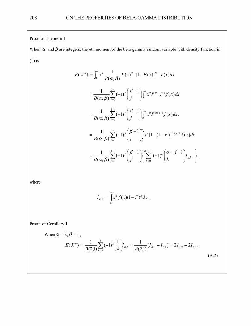
Proof of Theorem 1

When α and β are integers, the nth moment of the beta-gamma random variable with density function in

(1) is

)( nXE = 1 1

0

1 ( ) [1 ( )] ( )( , )

nx F x F x f x dxB

α β

α β∞ − −−∫

11

00

11 ( 1) ( )( , )

j n j

jx F F f x dx

jB

βαβ

α β

− ∞ −

=

−⎛ ⎞= − ⎜ ⎟

⎝ ⎠∑ ∫

1

1

00

11 ( 1) ( )( , )

j n j

jx F f x dx

jB

βαβ

α β

− ∞ + −

=

−⎛ ⎞= − ⎜ ⎟

⎝ ⎠∑ ∫ .

dxxfFxjB

jn

j

j )()]1(1[1

)1(),(

1 1

0

1

0

−+∞−

=

−−⎟⎟⎠

⎞⎜⎜⎝

⎛ −−= ∫∑ α

β ββα

1 1

,0 0

1 11 ( 1) ( 1)( , )

jj k

n kj k

jI

j kB

β αβ αα β

− + −

= =

⎧− + −⎛ ⎞ ⎛ ⎞ ⎫= − −⎨ ⎬⎜ ⎟ ⎜ ⎟

⎝ ⎠ ⎝ ⎠ ⎭⎩∑ ∑ ,

where

knI , dxFxfx kn∫∞

−=0

)1)(( .

Proof: of Corollary 1

When 1,2 == βα ,

=)( nXE knk

k IkB ,

1

0

1)1(

)1,2(1

⎟⎟⎠

⎞⎜⎜⎝

⎛−∑

=

][)1,2(

11,0, nn II

B−= 1,0, 22 nn II −= .

(A.2)


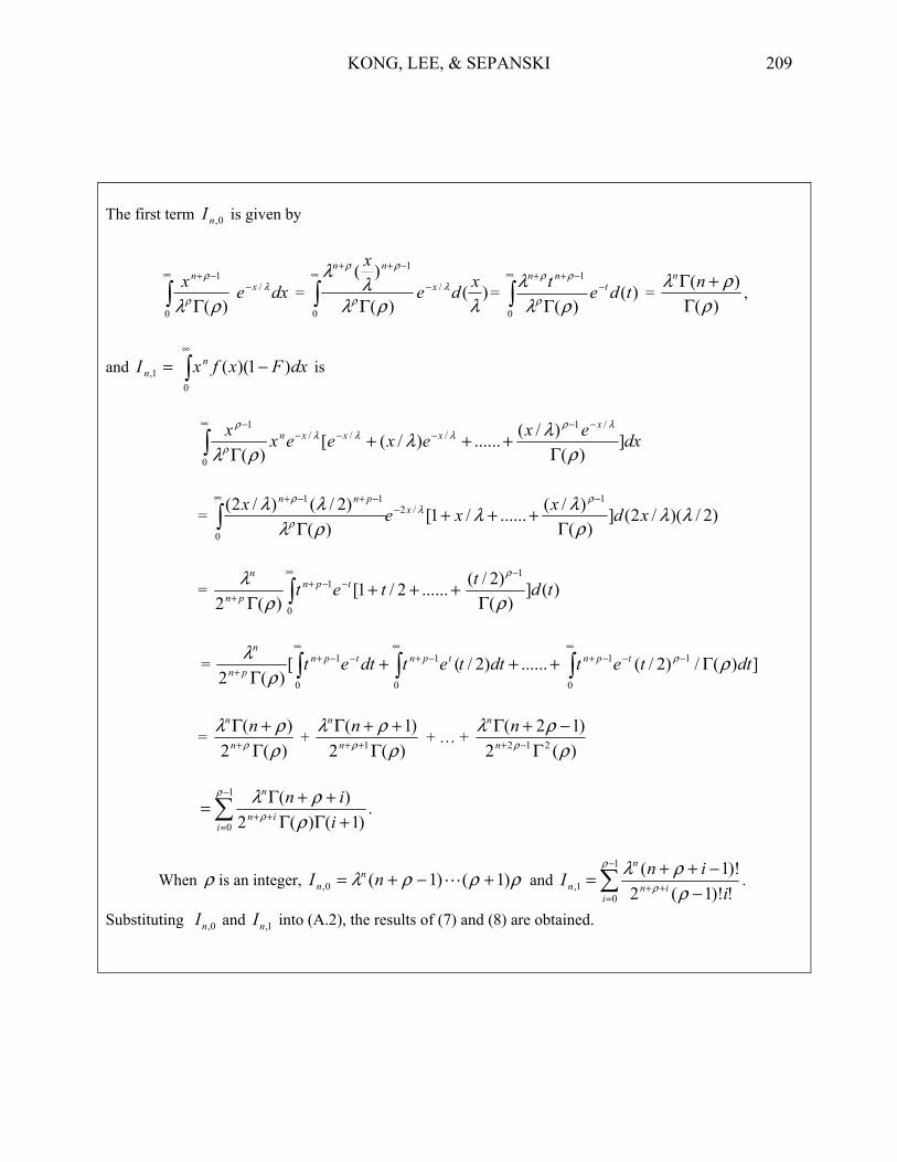
The first term 0,nI is given by

dxex xn

λρ

ρ

ρλ/

0

1

)(−

∞ −+

∫ Γ = )(

)(

)(

0

/

1

λρλλ

λλ

ρ

ρρ

xde

xx

nn

∫∞

−

−++

Γ= )(

)(0

1

tdet tnn

∫∞

−−++

Γ ρλλ

ρ

ρρ

= )(

)(ρ

ρλΓ

+Γ nn

,

and =1,nI ∫∞

−0

)1)(( dxFxfxn is

dxexexeexx xxxxn ]

)()/(......)/([

)(

/1///

0

1

ρλλ

ρλ

λρλλλ

ρ

ρ

Γ+++

Γ

−−−−−

∞ −

∫

= )2/)(/2(])(

)/(....../1[)(

)2/()/2( 1/2

0

11

λλρ

λλρλλλ ρ

λρ

ρ

xdxxex xpnn

Γ+++

Γ

−−

∞ −+−+

∫

= ∫∞

−−++ +++

Γ 0

1 ......2/1[)(2

tet tpnpn

n

ρλ )(]

)()2/( 1

tdtρ

ρ

Γ

−

= ∫ ∫∞ ∞

−+−−++ +++

Γ 0 0

11 ......)2/([)(2

dttetdtet tpntpnpn

n

ρλ ])(/)2/( 1

0

1 dttet tpn ρρ Γ−∞

−−+∫

= )(2)(

ρρλ

ρ Γ+Γ

+n

n n +

)(2)1(

1 ρρλ

ρ Γ++Γ

++n

n n + … +

)(2)12(

212 ρρλ

ρ Γ−+Γ

−+n

n n

∑−

=++ +ΓΓ

++Γ=1

0 )1()(2)(ρ

ρ ρρλ

iin

n

iin

.

When ρ is an integer, ρρρλ )1()1(0, +−+= nI nn and 1,nI ∑

−

=++ −

−++=1

0 !)!1(2)!1(ρ

ρ ρρλ

iin

n

iin

.

Substituting ,0nI and ,1nI into (A.2), the results of (7) and (8) are obtained.


210

Proof of Lemma 2:

(a) As x goes 0, 0lim ( )x H x→ is

∫ −−

−−

→

−−

−

xx

dxxfFFB

xfFFB

0

11

11

0

)()1(),(

11

)()1(),(

1

limβα

βα

βα

βα )(lim 0 xgx→= ,

which is given in Lemma 1.

Proof: (b) As x goes to ∞ , by L’Hospital Rule, )(lim xHx ∞→ is

limx→∞ fFFfFFfFFxfFxfF

11

'1122112

)1()1()()1)(1()()1)(()1(

−−

−−−−−−

−−−+−−−+−−

βα

βαβαβα βα

])()('

)(1)()1(

)()()1([lim

xfxf

xFxf

xFxf

x −−−+−= ∞→

βα

)()('lim

)()('lim)1(

10

xfxf

xfxf

xx ∞→∞→ −−

−+= β

)()('lim

xfxf

x ∞→−= βλρ

λρλρ

ρλβ x

xx

x

ex

exex

−−

−−

−−

∞→

−+−

−=1

21

)1(lim

)11(limxx−+−−= ∞→

ρλ

βλβ= .

Note that unlike 0lim ( )x H x→ , the limit )(lim xHx ∞→ = λβ / does not depend on α and ρ . In other word, the instantaneous failure rate will not depend on α and ρ in the long run.


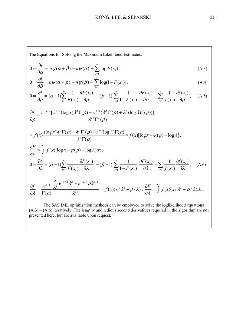
The Equations for Solving the Maximum Likelihood Estimates:

=∂∂=αl0 )( βαψ +n )(αψn− ∑

=

+n

iixF

1

)(log . (A.3)

=∂∂=βl0 )( βαψ +n )(βψn− ))(1log(

1∑

=

−+n

iixF . (A.4)

=∂∂=ρl0

ρα

∂∂

− ∑=

)()(

1)1(1

in

i i

xFxF

)1( −− β ∑= −

n

i ixF1 )(11

ρ∂∂ )( ixF

+ρ∂

∂∑=

)()(

11

in

i i

xfxf

, (A.5)

)())]()(log)('()()(log[

22

11/

ρλρλλρλρλ

ρ ρ

ρρρρρλ

ΓΓ+Γ−Γ=

∂∂ −−− xxxef x

)()()(log)(')()(log)(

ρλρλλρλρλ

ρ

ρρρ

ΓΓ−Γ−Γ= xxf = ]log)()[log( λψ −− pxxf ,

dxpxxfF x

]log)()[log(0

λψρ

−−=∂∂

∫ .

=∂∂=λl0

λα

∂∂

− ∑=

)()(

1)1(1

in

i i

xFxF

)1( −− β ∑= −

n

i ixF1 )(11

λ∂∂ )( ixF

+λ∂

∂∑=

)()(

11

in

i i

xfxf

, (A.6)

=∂∂λf

ρ

ρλρλρ

λ

ρλλλ

ρ 2

1//21

)(

−−−− −

Γ

xx eexx )//)(( 2 λρλ −= xxf ; dxxxfF x

)//)(( 2

0

λρλλ

−=∂∂

∫ .

The SAS IML optimization methods can be employed to solve the loglikelihood equations (A.3) – (A.6) iteratively. The lengthy and tedious second derivatives required in the algorithm are not presented here, but are available upon request.

on the properties of beta-gamma distribution · on the properties of beta-gamma distribution 188...

Documents