on the practical stability of hybrid control algorithm
TRANSCRIPT

HAL Id: hal-01730522https://hal.archives-ouvertes.fr/hal-01730522v2
Submitted on 17 Sep 2018
HAL is a multi-disciplinary open accessarchive for the deposit and dissemination of sci-entific research documents, whether they are pub-lished or not. The documents may come fromteaching and research institutions in France orabroad, or from public or private research centers.
L’archive ouverte pluridisciplinaire HAL, estdestinée au dépôt et à la diffusion de documentsscientifiques de niveau recherche, publiés ou non,émanant des établissements d’enseignement et derecherche français ou étrangers, des laboratoirespublics ou privés.
On the practical stability of hybrid control algorithmwith minimum dwell-time for a DC-AC converter
Carolina Albea-Sanchez, Oswaldo Lopez Santos, David A. Zambrano Prada,Francisco Gordillo, Germain Garcia
To cite this version:Carolina Albea-Sanchez, Oswaldo Lopez Santos, David A. Zambrano Prada, Francisco Gordillo, Ger-main Garcia. On the practical stability of hybrid control algorithm with minimum dwell-time fora DC-AC converter. IEEE Transactions on Control Systems Technology, Institute of Electrical andElectronics Engineers, 2019, 27 (6), pp.2581-2588. 10.1109/TCST.2018.2870843. hal-01730522v2
1
On the practical stability of hybrid control algorithmwith minimum dwell-time for a DC-AC converterCarolina Albea Sanchez, Oswaldo Lopez Santos, David. A. Zambrano Prada, Francisco Gordillo, Germain
Garcia
Abstract—This paper presents a control law based on HybridDynamical Systems (HDS) theory for a dc-ac converter. Thistheory is very suited for analysis of power electronic converters,since it combines continuous (voltages and currents) and discrete(on-off state of switches) signals avoiding, in this way, the use ofaveraged models. Here, practical stability results are induced forthis tracking problem, ensuring a minimum dwell-time associatedwith an LQR performance level during the transient responseand an admissible chattering around the operating point. Theeffectiveness of the resultant control law is validated by meansof simulations and experiments.
I. INTRODUCTION
The control of power converters is characterized by the factthat the input signals are discrete, since they are the on-offstate of switching devices, while the rest of signals, includingthe ones to be controlled, are continuous. However, most of themethods for the control of power converters use an averagedmodel in which the discrete signals are averaged during eachsampling period and, thus, are considered continuous signals[1]–[3]. These approaches have solved many practical prob-lems in terms of theoretical justifications, but the answers stillare incomplete to some extent. Among the main limitations,we can point out the difficulty of quantifying the precision ofthe approximation, resulting from the averaging procedure andthe fact that the properties of the control laws are only validlocally. More recently, the control community has concentratedefforts on the study of new hybrid control techniques. Indeed,Hybrid Dynamical Systems (HDS) framework is suitable formodelling and controlling this kind of systems, because it al-lows guaranteeing a global stability improving power converterperformance, as the reduction of switching, for instance.
The HDS framework was firstly applied to electronic con-verters in 2003 [4] and after that more applications haveappeared [5]–[7]. All these applications consider dc-dc con-verters, whose objective, from the control theory point ofview, is to stabilize an operating point. Nevertheless, in otherelectronic converters is usual to work with ac and thus, theproblem is more involved. When ac voltage is to be generated,as is the case of inverters, the objective is to track a sinusoidalreference. There exist some works dealing with this problem.For example, in [8], [9] authors provide a hybrid algorithm
Carolina Albea Sanchez and Germain Garcia are with LAAS-CNRS, Uni-versite de Toulouse, CNRS, Toulouse, France, e-mail: calbea,[email protected]
Oswaldo Lopez Santos and David. A. Zambrano Prad are with University ofIbague, Colombia, e-mail: oswaldo.lopez,[email protected]
Francisco Gordillo is with University of Seville, Spain, e-mail:[email protected]
This work has been partially funded under grants MINECO-FEDERDPI2013-41891-R and DPI2016-75294-C2-1-R.
and a hybrid predictive control, respectively, for controllinga DC/AC converter with a minimum dwell-time, which isguaranteed using a space regulation. However, this dwell-timewas not quantized in time for physical implementation issues.Likewise, the authors do not provide experiments to validatethe controlled system.
A preliminary version of this paper appeared in [10] wherea tradeoff between the switching frequency and performancewas considered using a tuning parameter. In this new version,a modification of the control law is proposed in order to avoidinfinitely fast switching in steady state, which is not desirablefor energy efficiency and reliability considerations. Further-more, practical stability proofs are now included. Experimentsin a prototype validate the results.
The rest of the paper is organized as follows. The half-bridge inverter model is described in Sect. II while the controlproblem is stated in Sect. III. In Sect. IV a hybrid versionof the model is proposed as well as the hybrid control law.Uniform Global Asymptotic Stability is proved. In Sect. V itis shown that one of the parameters of the control law can beused to cope with a tradeoff between dwell-time –and, thus, theswitching frequency– and an LQR performance measurement.Section VI presents a modification of the control law in orderto avoid infinitely fast switching at steady state. Simulationsare presented in Sect. VII, and experiment results are presentedin Sect. VIII. The paper closes with a section of conclusionsand future work.
Notation: Through out the paper R denotes the set of realnumbers, Rn the n-dimensional euclidean space and Rn×mthe set of all real n×m matrices. The set of non-negative realnumbers is denoted by R≥0. M 0 (resp. M ≺ 0) representsthat M is a symmetric positive (resp. negative) definite matrix.The Euclidan norm of vector x ∈ R is denoted by |x|. I isthe identity matrix of appropriate dimension. λm(M), λM (M)represent the minimum and maximum eigenvalues of M .
II. HALF-BRIDGE INVERTER MODEL
Among the well-known inverter topologies used in single-phase stand-alone applications, the simpler one regarding thenumber of power semiconductors is the half-bridge converter.This converter feeds a resistive load R0, from a regulated DCsource (2Vin) as depicted in Fig. 1. The resonant LC filteris used to increase the fundamental component amplitude,attenuating simultaneously the high frequency components.RLS gathers the main conduction losses.
Assumption 1. Load R0 and voltage input 2Vin are con-sidered constant. We also regard C1 = C2, which are large

2
enough, such that the voltage ripple is negligible (vC1= vC1
and vC2 = vC2 ) and input voltage is symmetrically distributedamong them (vC1 = vC2 = Vin). Therefore, the capacitordynamics are not considered in the following. Moreover,variables iL and vC are measurable.
A. System description
The system differential equations can be written as
d
dt
[iL(t)vC(t)
]=
[−RLS
L − 1L
1C0
− 1R0C0
] [iL(t)vC(t)
]+
[Vin
L0
]u (1)
where iL is the inductance current, vC is the capacitor voltage.Moreover, u = U1 − U2 ∈ −1, 1 is the control inputwhich represents two operating modes. The first one, u = −1,corresponds to U1 = 0 (U1 OFF) and U2 = 1 (U2 ON). Andthe second one, u = 1, corresponds to U1 = 1 (U1 ON) andU2 = 0 (U2 OFF). Note, that due to the converter objectivevC and iL are alternating voltage and current, respectively.
From a control point of view, the general control objectiveof this class of inverter is to stabilize system (1) in a desiredoscillatory trajectory. That means, controlling the invertersuch that its output voltage asymptotically tracks a sinusoidalreference.
Figure 1: Half-bridge inverter.
With this goal let us consider system (1) described by thefollowing state-space equations:
x = Ax+Bu (2)
where x = [iL vC ]T are continuous-time variables represent-ing the internal states, and they are assumed to be accessible,allowing to consider that x is the system output. u ∈ −1, 1is the discrete-time variable corresponding to the control input.Note that A, B and C are matrices of appropriate dimensions.
The control objective mentioned above is to control theinverter in order to follow a desired trajectory on vC definedby
vCd(t) = Vmax sin(ωt). (3)
Vmax is the desired amplitude of the voltage through the loadR0. A simple circuit analysis shows that if in steady statevC = vCd
, the current iL in the inductance is given by
iLd(t) = C0ωVmax cos(ωt) +
VmaxR0
sin(ωt). (4)
III. PROBLEM STATEMENT
The objective of this work is to stabilise the half-bridgeinverter in a limit cycle given by (3)–(4). To impose such abehavior, let us drive system (2) by an exogenous input z ∈ R2
generated by the next linear time-invariant exosystem:
z =
[0 −ωω 0
]z = Θz z(0) =
[0
Vmax
]. (5)
Remark 1. From (5) it is simple to see that for all t ∈ R≥0
z21(t) + z2
2(t) = V 2max.
Then, let us define the compact set
Φ = z21 + z2
2 = V 2max, (z1, z2) ∈ R, Vmax ∈ R. (6)
Note, from Remark 1, that we can reformulate our trackingproblem, as a regulation problem, defining the dynamics ofthe overall system as
x = Ax+Buz = Θzx = x+Dz = x−Πz,
(7)
where x ∈ R2 is the tracking error, D = −Π being Π definedfrom (3) and (4) as:
Π :=
[ωC0
1R0
0 1
].
Then, from (7) and choosing
Γ :=[Γ1 Γ2]
=[
ωLR0Vin
+ wRLSC0
Vin
(1L − C0ω
2 + RLS
LR0
)LVin
], (8)
the tracking error dynamic is given by
˙x = x−Πz = Ax+Bu−ΠΘz
= A(x+ Πz) +Bu−ΠΘz ±BΓz
= Ax+Bv. (9)
being AΠ +BΓ = ΠΘ and
v := u− Γz. (10)
Remark 2. Note that the algebraic equations deduced from(7) and (9)
AΠ +BΓ = ΠΘ. (11)CΠ +D = 0 (12)
are involved in the well-known “regulator equation”, [11].
Then, let us define the compact set:
Υ := v = u− Γz, u ∈ −1, 1, z ∈ Φ,Γ ∈ R1×2.
Assumption 2. In (7), vCdis supposed to be measurable as
a reference in such a way that it is desired that the inverterproduces a voltage with the same amplitude, frequency andphase. Then, z can be internally reconstructed, as it is shownin Fig. 2.
The aim of this work can now be stated.

3
vCd Recons.
Control DC/ACu
z iL
vCz
Figure 2: Block diagram of the hybrid controlled inverter.
Problem 1. Design a control law v (or equivalently u) suchthat for any initial condition x(0) ∈ R2:• the trajectory of (9) is bounded,• limt→∞ x(t) = 0,• a minimum dwell-time, in the transient time as well as
in the steady state, is guaranteed to avoid infinite fastswitching.
• it is possible to deal with the tradeoff between a mini-mum dwell-time and, an LQR performance level (in thetransient time), as well as, with the tradeoff between aminimum dwell-time and the size of the asymptoticallystable set around the compact set (6) (in the steady state).
To solve Problem 1, we use the main idea proposed in [7],formulating the problem under a hybrid dynamical frameworkfollowing the theory given in [12], where continuous-timebehaviour follows the evolution of the voltage and current in(1), and the discrete-time behaviour captures the switching ofthe control signal u. Likewise, we remark that the problem isan output regulation problem and the idea here is also inspiredby the work in [11].
IV. HYBRID MODEL AND PROPOSED CONTROL LAW
Let us recall that error dynamics are described by
˙x = Ax+Bv,z = Θz,
(13)
where the available input v given in (10) is composed of acontinuous-time signal Γz and a switching signal u, whichcan achieve a logical mode between 2 possible modes
u ∈ −1, 1. (14)
This paper focuses on the design of a control law for theswitching signal u, in order to ensure suitable convergenceproperties of the inverter error variable x to 0. Following theworks shown in [6], [7], [13], we represent in the followingassumption a condition that characterizes the existence of asuitable switching signal inducing x = 0.
Assumption 3. Given a matrix Q 0, there exists a matrixP 0 such that:
1) matrix A verifies
ATP + PA+ 2Q ≺ 0, (15)
2) for any z ∈ Φ, there exist λ1,e(t), λ−1,e(t) ∈ [0, 1]satisfying λ1,e + λ−1,e = 1, such that,
λ1,e − λ−1,e − Γz = 0. (16)
Note that the solution x = 0 to (13) with (10) is admissibleif it is an equilibrium for the averaged system ˙x = Ax +B(λ1,e − λ−1,e − Γz). Note that the average dynamics canbe perceived as the result of arbitrarily fast switching and asrelaxations in the generalized sense of Krasovskii or Filippov,because (16) means that in x = 0 the signal is a periodicsequence of arbitrarily small period T , spending a time equalto λ1,eT in mode u = 1, and λ−1,eT in mode u = −1.
In order to present the proposed control law, consider thefollowing HDS model:
H :
˙xzv
= f(x, z, v), (x, z, v) ∈ Cx+
z+
v+
∈ G(x, z), (x, z, v) ∈ D,
(17)
where G is a set-valued map representing the switching logic:
f(x, z, v) :=
Ax+BvΘz−ΓΘz
G(x, z) :=
xz(
argminu∈−1,1
xTP (Ax+B(u− Γz))
)− Γz
(18)
and where the flow and jump sets C and D encompass,respectively, the regions in the (extended) space (x, z, v) whereour switching strategy will continue with the current mode vwhen the states are in set C or will be require to switch toa new mode when the states are in set D. If (x, z, v) ∈ Dthen u will switch according to G in (18) given the value ofv = u− Γz.
Based on the parameters P and Q introduced in Assump-tion 3, we select the following flow and jump sets:
C := (x, z, v) : xTP (Ax+Bv) ≤ −ηxTQx (19)D := (x, z, v) : xTP (Ax+Bv) ≥ −ηxTQx, (20)
where η ∈ (0, 1) is a useful design parameter allowing todeal with a tradeoff between an LQR performance level andswitching frequency, as characterized below in Theorem 2.
Proposition 1. The hybrid dynamical system (17)–(20) sat-isfies the basic hybrid conditions [12, Assumption 6.5], andthen it is well-posed.
Proof. To prove the hybrid basic conditions we see that thesets C and D are closed. Moreover f is a continuous function,thus it trivially satisfies outer semicontinuity and convexityproperties. The map G is closed, therefore it also is outersemicontiunuous [12, Lemma 5.1] and, f and G are locallybounded. Finally, the second conclusion of the propositioncomes from [12, Theorem 6.30].
Now, we evoke Lemma in [7, Lemma 1], which is funda-mental to stablish Theorem 1.

4
Lemma 1. Consider that all conditions of Assumption 3 aresatisfied. Then, for each x ∈ R2,
minu∈−1,1
xTP (Ax+B(u− Γz)) ≤ −xTQx. (21)
Proof. Define the compact set
Λ = λ−1, λ1 ∈ [0, 1] : λ−1 + λ1 = 1 .
Then, the following minimum is obtained at the extremepoints:
minu∈−1,1
xTP (Ax+Bu−BΓz)
= minλ1,λ−1∈Λ
xTP (Ax+Bλ1 −Bλ−1 −BΓz) ≤ −xTQx,
where in the last step we used relations (15) and (16) .
The switching signals generated by our solution will dependon Lemma 1. Indeed, Assumption 3 with (19) shows thatunless x = x+ = 0, the solution always jumps to the interiorof the flow set C because
−xTQx < −ηxTQx,
and η < 1.Following up, we will establish uniform stability and con-
vergence properties of the hybrid system (17)–(20) to thecompact attractor
A := (x, z, v) : x = 0, z ∈ Φ, v ∈ Υ, (22)
where the sets Φ and Υ are defined in Remark 1 and 2,respectively.
Theorem 1. Under Assumptions 2,3 the attractor (22) isuniformly globally asymptotically stable (UGAS) for hybridsystem (17)–(20).
Proof. Let us take the Lyapunov function candidate
V (x) =1
2xTPx. (23)
In the flow set, C, using its definition in (19), we have
〈∇V (x), f(x, z, v)〉 = xTP (Ax+Bv) ≤ −ηxTQx. (24)
Across jumps we trivially get:
V (x+)− V (x) =1
2
(x+)TPx+ − xTPx
= 0, (25)
because x+ = x.Uniform global asymptotic stability is then proved applying
[14, Theorem 1] to the incomplete Lyapunov function, V .Indeed, for a fixed Γ, which is defined in (8) and Vmax, zand v are bounded and evolve in the interior of the attractorA, being their distances to the attractor 0. Likewise, since thedistance of x to the attractor (22) is defined by |x| = |x|A,we have that [14, eq. (6)] holds from the structure of V andfrom (24) and (25). [14, Theorem 1] also requires building the
restricted hybrid system Hδ,∆ by intersecting C and D withthe set
Sδ,∆ = (x, z, v) : |x| ≥ δ and |x| ≤ ∆
and then proving (semi-global) practical persistence flowfor Hδ,∆(f,G,C ∩ Sδ,∆, D ∩ Sδ,∆), for each fixed values of(δ,∆). In particular, practical persistent flow can be guaranteedby showing that there exists γ ∈ K∞ and M ≥ 0, such that,all solutions to Hδ,∆ satisfy
t ≥ γ(j)−M, ∀(t, j) ∈ dom ξ (26)
where ξ = (x, z, v) and
dom ξ =⋃
j∈domj ξ
[tj , tj+1]× j (27)
is the hybrid time domain (see [12, Ch. 2] for details). Toestablish (26), notice that after each jump, from the definitionof G in (18) and from property (21) (in Lemma 1), we have
xTP (Ax+Bv+) ≤ −xTQx < −ηxTQx, (28)
where we used the fact that η < 1 and that (0, z, v) /∈ Sδ,∆.Therefore, if any solution to Hδ,∆ performs a jump from
Sδ,∆, it will remain in Sδ,∆ (because x remains unchanged)and then, from (20), it jumps to the interior of the flow setC ∩Sδ,∆. Moreover, from the strict inequality in (28), then allnon-terminating solutions must flow for some time and sinceC ∩ Sδ,∆ is bounded, there is a minimum uniform dwell-timeρ(δ,∆) between each pair of consecutive jumps. In particular,this dwell-time is lower-bounded by a constant, which isdirectly related in the state-space by an upper-bound of V (x)and 〈∇V (x), f(x, z, v+)〉, which are V (x) ≤ λm(P )δ2 and〈∇V (x), f(x, z, v+)〉 ≤ −(1− η)λm(Q)δ2, respectively.
This dwell-time (δ,∆) clearly implies [14, eq. (4)] γ(j) =ρ(δ,∆)j (which is a class K∞ function) and M = 1. Then,all the assumptions of [14, Theorem 1] hold and UGAS of Ais concluded.
Corollary 1. The hybrid dynamical system (17)–(20) is UGASand is robust with respect to the presence of small noise in thestate, unmodeled dynamics, and time regularization to relaxthe rate of switching, because the attractor (22) is compact.
Proof. From Theorem 1, we prove that the hybrid dynamicsystem is UGAS, and from Proposition 1 we see that it iswell-posed. Moreover, as the attractor (22) is compact then itis robustly KL asymptotically stable in a basin of attraction[12, Chapter 6].
Remark 3. Note that according to Theorem 1 system (17)–(20) may exhibit a Zeno behaviour when x 7→ 0, and con-sequently an infinitely fast switching may be expected, whichis not acceptable in practice. This will be practically avoidedlater introducing an additional dwell-time logic to obtain atemporal-regularisation of the dynamics, thereby weakeningasymptotic convergence into practical convergence.
Remark 4. The implementation of this control law is verysimple and requires a low computational cost. The control
5
law is implemented in the interior of the assigned block inFig. 2, as follow: we initialize the constant parameters, andfrom the inputs, we check if the condition of the jump flow, D isverified. If it is the case, system jumps to the other functioningmode, because from Lemma 1 and from the fact that there arejust two functioning modes, the other mode will correspond tothe map of v given in G.
V. TRADEOFF BETWEEN DWELL-TIME AND LQRPERFORMANCE
Once that UGAS property of the attractor is established forour solution, we focus on providing a suitable performanceguarantee in order to reduce, for instance, the energy cost,current peaks and response time for the voltage or current.For this goal we apply the same paradigm shown in [7] for ahybrid context applied to switched systems.
Within the considered hybrid context, we recall that thesolutions parametrized in a hybrid time domain domj ξ cor-responds to a finite or infinite union of intervals of theform (27). Within this context, we represent a quadratic LQRperformance metric focusing on flowing characteristics of theplant state, using the expression∑
k∈domj ξ
∫ tk+1
tk
xTCTCxdτ, (29)
where ξ = (x, z, v) : dom ξ → Rn×Rn×Rn is a solution tohybrid system (17)–(20), for all (t, j) ∈ dom ξ.
The following theorem guarantees a maximum performancecost (29) for our hybrid system.
Theorem 2. Consider hybrid system (17)–(20) satisfyingAssumptions 2,3. If
Q ≥ I, (30)
then the following bound holds along any solution ξ =(x, z, v) of (17)–(20):
J(ξ) ≤ 1
2ηx(0, 0)TPx(0, 0), (31)
for all (t, j) ∈ dom(ξ).
Proof. To prove the LQR performance bound given in (31),consider any solution ξ = (x, z, v) toH. Then for each (t, j) ∈dom ξ and denoting t = tj+1 to simplify notation, we havefrom (24)
V (x(t, j))− V (x(0, 0))
=
j∑k=0
V (x(tk+1, k))− V (x(tk, k))
=
j∑k=0
∫ tk+1
tk
〈∇V (x(τ, k)), f(x(τ, k), z(τ, k), v(τ, k))〉dτ
≤j∑
k=0
∫ tk+1
tk
−ηxT (τ, k)Qx(τ, k)dτ
≤ −ηj∑
k=0
∫ tk+1
tk
xT (τ, k)x(τ, k)dτ, (32)
where the last inequality comes from applying (30). Now,taking the limit as t + j → +∞ and using the factthat the UGAS property established in Theorem 1 implieslimt+j→+∞ V (x(t, j)) = 0, we get from (32)
ηJ(ξ) ≤ V (x(0, 0)) =1
2x(0, 0)TPx(0, 0),
as to be proven.
Remark 5. Note that for a given P and Q that satisfy (30), theguaranteed performance level is proportional to the inverse ofη ∈ (0, 1). That means that large values of η are expected todrive to improved LQR performance along solutions.
On the other hand, note from the flow and jump sets in(19) and (20), that larger values of η (close to 1) correspondto strictly larger jump sets (and smaller flow sets), whichreveals that solutions with larger values of η exhibit a largerswitching frequency. In other words, through parameter η wecan deal with a tradeoff between switching frequency and anLQR performance level given in (31).
A. Computation of P and Q
Now, we address the problem of the computation of param-eters P , Q, following any class of optimization that reducesas much as possible the right hand side in bound (31) withany Q ≥ CTC. To this end, we select the cost function asfollows [7, Section IV]:
J(ξ) := minu
∑k∈domj(ξ)
∫ tk+1
tk
(ρ
R0(vC(τ, k)− vCd
)2
+ RLS(iL(τ, k)− iLd)2)dτ,
where ρ is a positive scalar. Note that the constant parametersof each term express the energy weighted sum of the errorsignal for each state variable. From this, we take
Q =
[RLS 0
0 ρR0
]such that, all assumptions of Theorem 2 are satisfied.
Once Q is selected, and noting that matrix A is Hurwitz, thefollowing convex optimization expressed by the linear matrixinequality always leads to a feasible solution
minP=PT>0
TraceP, subject to: (33)
ATP + PAT + 2Q ≺ 0,
and this optimal solution clearly satisfies (15).
VI. PRACTICAL GLOBAL RESULTS USINGTIME-REGULARIZATION
The hybrid control law proposed above can exhibit infinitelyfast switching at steady state, because given an initial conditionin A, one sees that the hybrid dynamics (17)–(20) haveat least one solution that keeps jumping onto A. Infinitelyfast switching is not desirable in terms of energy efficiencyand reliability, because every switch dissipates energy andreduces the switch lifespan. For this reason, we propose afew modifications of the hybrid law, aiming at reducing the

6
frequency switching when e is close to zero. This goal isreasonable for the proposed law, because it is possible to showthat away from A, our control law already joins a desirableproperty of minimum dwell time between switching, as longas Assumption 3 holds. For this, given any vCd
, iLdand P,Q
satisfying the above assumptions, consider system (17)–(20)and denote it by the shortcut notation H := (f,G, C,D)and then, for a non-negative scalar T and introducing thefollowing additional state variable τ to dynamics (17), definethe following time-regularized version of H:
HT :
[˙xzv
]= f(x, z, v),
τ = 1− ς(τT
),
(x, z, v) ∈ CT[x+
z+
v+
]∈ G(x, z),
τ+ = 0,(x, z, v) ∈ DT ,
(34a)where the ς denotes the non-negative side of the unit deadzonefunction defined as ς(s) := max0, s−1, for all s ≥ 0 and thejump and flow sets are the following time-regularized versionsof C and D in (17)–(20):
CT := C × [0, 2T ] ∪ (x, z, v, τ : τ ∈ [0, T ]DT := D × [T, 2T ].
(34b)
The above regularization is clearly motivated by the attemptthat all solutions are forced to flow for at least T ordinarytime after each jump. Therefore, there are not jumps when thetimer τ is too small. Note also that the deadzone given by ςallows a solution to flow forever while ensuring that timer τremains in a compact set.
The introduction of the time regularization term in (34a)presents the following consequences:• It modifies the attractor set defined in (22). Now the new
attractor can be characterized by
AT := (x, z, v, τ) : ‖x‖ ≤ X, z ∈ Φ, v ∈ Υ, τ ∈ [0, 2T ].(35)
• Attractor (35) is UGAS for sufficiently small values ofT > 0. Remark that attractor (35) tends to attractor (22)as T tends to zero.
To show the previous statement and give an interval of valuesof T ensuring UGAS, let us consider the following lemma[15, Theorem 3.2.2], whose proof is given for the sake ofcompleteness.
Lemma 2. Consider Assumption 3 is satisfied, then all theeigenvalues of the matrix P−1Q are positive and
‖eAt‖ ≤λ
1/2M (P )
λ1/2m (P )
e−αt
where α = λm(P−1Q).
Proof. Let us multiply (15) by P−1/2 on the right and onthe left side, and define F := P 1/2AP−1/2 and α :=λM (P−1/2QP−1/2), then we obtain:
FT + F ≤ −2P−1/2QP−1/2 ≤ −2αI. (36)
Let us now define the function ζ(t) := ‖e(F+αI)tx‖2. Then,from (36), we have
dζ
dt= xT e(F+αI)t(FT + F + 2αI)e(F+αI)tx ≤ 0.
Therefore, we can remark that ζ is a non-increasing functionand
‖e(F+αI)tx‖2 = ζ(t) ≤ ζ(0) = ‖x‖2, ∀t ≥ 0.
Note that this last condition can also be rewritten as
‖e(F+αI)tx‖‖x‖
≤ 1
which implies
‖e(F+αI)t‖ ≤ 1 ⇔ ‖eFt‖ ≤ e−αt, ∀T ≥ 0. (37)
On the other hand, from F definition and classical mathe-matical manipulations, we get eAt = P−1/2eFtP 1/2. Then,
‖eAt‖ = ‖P−1/2eFtP 1/2‖ ≤ ‖P−1/2‖‖P 1/2‖‖eFt‖≤ ‖P−1/2‖‖P 1/2‖e−αt.
Note that last inequality is achieved from using (37).Let us apply ‖P 1/2‖2 = λM (P ) and ‖P−1/2‖2 = λ−1
m (P )which gives
‖eAt‖ ≤λ
1/2M (P )
λ1/2m (P )
e−αt ∀t ≥ 0.
Now remark that P−1/2QP−1/2 = P 1/2[P−1Q]P−1/2 >0 and thus, P−1/2QP−1/2 presents the same eigenvaluesas P−1Q. Then from (36), α = λm(P−1/2QP−1/2) =λm(P−1Q) and the proof is complete.
Now, we establish a useful practical minimum dwell-timeproperty for HT .
Property 1. There exists a positive scalar T ∗, such that forany chosen T ≤ T ∗ the solutions (t, j) → ξ(t, j) to hybridsystem (34) flow for at least T ordinary time after the jumpbefore reaching set DT . Moreover, as T tends to zero, theminimum dwell time tends to zero as well.
Proof. From Theorem 1, we guarantee that for all solutions farenough from A, there exists a minimum dwell- time managedby η, as discussed in Remark 3. Consider the hybrid system(34) between two jumps in the neighbourhood of A. Withoutloss of generality, consider that the first jump occurs at timet = t0 and let us consider the variable t := t − t0. Then, inthe flow set CT , the trajectories are described by:
˙x(t) = Ax(t) +Bu−BΓz(t), x(0) = x0
for a given T > 0.From (5), note that the trajectories of z are
z(t) =
[z1(t)z2(t)
]=
[Vmax sin(ωt)Vmax cos(ωt)
]. (38)
Consequently, we can deduce that:
x(t) = eAt(x0+A−1B(u−W (t)))−A−1B(u−W (t)
)(39)
for 0 ≤ t ≤ T and with
W (t) = Vmaxρ1(ω) cos(ωt+ φ1(ω)
)+ Vmaxρ2(ω) sin
(ωt+ φ2(ω)
)

7
which is a bounded function with
ρ1(ω) = |(jωI −A)−1BΓ1|ρ2(ω) = |(jωI −A)−1BΓ2|φ1(ω) = arg(jωI −A)−1BΓ1)
φ2(ω) = arg(jωI −A)−1BΓ2).
Note that Γ1 and Γ2 come from (8).Let rewrite (39) as
x(t) +A−1B(u−W (t)) = eAt(x0 +A−1B(u−W (t))).
From the properties of a norm, we have:
‖x(t)+A−1B(u−W (t))‖ ≤ ‖eAt‖‖(x0+A−1B(u−W (t)))‖
and applying Lemma 2, we get,
‖x(t)−A−1B(u−W (t))‖ ≤λ
1/2M (P )
λ1/2m (P )
e−αt‖(x0 +A−1B(u−W (t)))‖.
Now, for 0 ≤ t ≤ T , we obtain
1 ≤ eαt ≤λ
1/2M (P )
λ1/2m (P )
‖x0 +A−1B(u−W (t))‖‖x(t)−A−1B(u−W (t))‖
and for all t > 0 and x(t) ∈ CT , we have
0 ≤ t ≤ 1
αLn
(λ
1/2M (P )
λ1/2m (P )
‖x0 +A−1B(u−W (t))‖‖x(t)−A−1B(u−W (t))‖
).
Let us consider that the next jump occurs at time t = T ,such that (x(T ), z(T ), v(T )) ∈ DT . Then for such T , we have
x(τ)TP (Ax(τ) +Bv(τ)) = −ηx(τ)TQx(τ)
and τ ∈ [T, 2T ].
or\andx(τ)TP (Ax(τ) +Bv(τ)) ≤ −ηx(τ)TQx(τ)
and τ = T.
Consequently, there exists a maximum dwell time bounddefined by T ∗ which satisfies:
T ∗ =1
αLn
(λ
1/2M (P )
λ1/2m (P )
‖x0 +A−1B(u−W (T ∗))‖‖x(T ∗)−A−1B(u−W (T ∗))‖
),
such that,0 ≤ T ≤ T ∗.
Note that x0 and x(T ) define the maximum possible chat-tering in the system induced by the dwell time bound, T ∗.
Property 1 ensures that some minimum dwell-time is guar-anteed if solutions remain sufficiently far from A. Moreover,using this property, the following desirable results are enjoyedby hybrid system HT .
Theorem 3. Consider a λ1, λ−1 and matrices P 0 andQ 0 satisfying Assumption 3. The following holds:
1) all solutions to HT enjoy a minimum dwell-time prop-erty with a minimum T ;
2) set AT in (35) is compact for any positive scalar T ≤T ∗.
3) for any positive scalar T ≤ T ∗, set AT in (35) is UGASfor dynamics HT in (34);
4) set A×0 is globally practically asymptotically stablefor (34), with respect to parameter T (namely as longas T is sufficiently small, the UGAS set AT in (35) canbe made arbitrarily close to A× 0.
Proof. Note that hybrid system (34) enjoys the hybrid basicconditions of [12, As. 6.5], because sets CT and DT areboth closed and f and G enjoy desirable properties. Then wemay apply several useful results pertaining well-posed hybridsystems (specifically, in the proof of item 2 below).
Proof of item 1. Note that the solutions present a minimumdwell-time property because the jumps are forbidden, at least,until the timer variable τ has reached the value T . Since τ = 1for all τ ≤ T , then all solutions flow for at least T ordinarytime after each jump (because τ+ = 0 across jumps).
Proof of item 2. Note that the hybrid system (34) satisfiesProperty 1. From this property is easy to see that x is boundedin the flow set CT . Indeed, from (39) and the properties of anorm, we have
‖x(t)‖ ≤ ‖eAt‖‖(x0 +A−1B(u−W (t)))‖+ ‖A−1B(u−W (t))‖
and applying Lemma 2 and the variable change t = t− t0, weobtain
‖x(t)‖ ≤λ
1/2M (P )
λ1/2m (P )
e−αt‖(x0 +A−1B(u−W (t)))‖
+ ‖A−1B(u−W (t))‖ := X, ∀t ≥ t0,
proving attractor AT is compact.Proof of item 3. From V (x) given in (23), and the bound
given before ‖x(t)‖ ≤ X , consider the following Lyapunovfunction candidate:
VT (x) = maxV (x)− λm(P )X2, 0, (40)
which is clearly positive definite with respect to AT andradially unbounded. Since outside set AT the hybrid dynamicsHT coincides with the one of H, then equations (24) and (25)hold for any (x, z, v) not in AT , which implies that
〈∇VT (x), f(x, z, v)〉 < 0 ∀x ∈ CT \ AT (41)VT (x+)− VT (x) = 0, ∀x ∈ DT \ AT . (42)
Moreover, from the property established in item 1, all completesolutions to HT must flow for some time, and thereforefrom (41), we have that no solution can keep VT constantand non-zero. UGAS of AT by applying the nonsmoothinvariance principle in [16], also using the well posednessresult established at the beginning of the proof.
Proof of item 4. Item 4 follows straightforwad recallingProperty 1, the minimum dwell time converges to zero as Tgoes to zero. Consequently, set AT in (35) shrinks to A×0as T goes to zero, and since we prove in item 2 that AT exists,we can make AT arbitrarily close to A× 0 by selecting Tsufficiently small.
8
Remark 6. Note that all solutions to the hybrid dynamicalsystem (34) present a minimum dwell-time in the ordinary time,given by T . This minimum dwell-time is not constant. Indeed,it increases if the solution does not satisfy any condition of DT .More precisely, the dwell-time is managed by η and eventuallyby T , if solutions are far from the attractorAT . In other words,if x is far from 0, then the rule xTP (Ax+Bv) ≥ −ηxTQxand the rule τ ∈ [T, 2T ] induce the dwell time. On the otherhand, the dwell-time is mainly managed by T , if solutions areclose to the attractor AT ; that means, if solutions are closeto x = 0, then the rule τ ∈ [T, 2T ] mainly induces the dwell-time.
The implementation of the hybrid system HT follows theprocedure given in Remark 4.
VII. SIMULATION
Table I: Simulation parameters
Parameter Convention Value UnitsDC input voltage Vin 48 V
Reference peak voltage Vmax 120√
2 VNominal angular frequency ω 2π (60) rad/s
Inductor L 50 mHOutput capacitor C0 140.72 µFLoad resistance R0 240 Ω
Estimated series resistance RLS 1.5 Ω
In this section, we validate in simulation the hybrid con-troller designed in this paper for the inverter given in (1).From parameters given in Table I and from (3) and (4) we gotthe following desired behaviour
xd =
[iLd
vcd
]=
[9 sin(2π60t+ 86)
120√
2 sin(2π60t)
], (43)
where it was applied the trigonometric relationship: a cos(x)+b sin(x) =
√(a2 + b2) sin(x + atan( ba )). Moreover, we take
ρ = 1000 and P =
[24.71 0.100.10 0.07
]. T ∗ is computed consid-
ering a chartering of iC equal to 2A and a chattering of vCequal to 10V , giving T ∗ = 0.041.
First, note that condition (15) is satisfied. Moreover, from(1), (3), (4) and the convex combination u = λ1 − λ−1 withλ1 + λ−1 = 1, we can achieve x = xd with λ1,e = 0.5 +0.003 sin(2π60t)+0.34 cos(2π60t), satisfying condition (16).
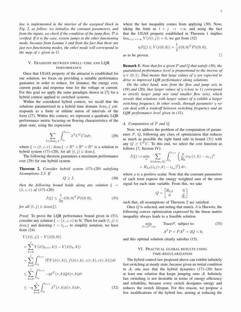
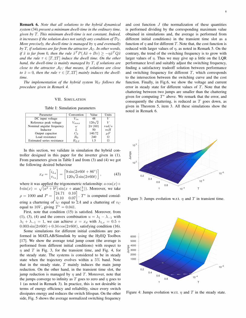
Some simulations for different initial conditions are per-formed in MATLAB/Simulink by using the HyEQ Toolbox[17]. We show the average total jump count (the average isperformed from different initial conditions) with respect toη and T in Fig. 3, for the transient time, and Fig. 4, forthe steady state. The systems is considered to be in steadystate when the trajectory evolves within a 5% band. Notethat in the steady state, T mainly induces the main jumpreduction. On the other hand, in the transient time slot, thejump reduction is managed by η and T . Moreover, note thatthe jumps converge to infinity as T goes to zero and η goes to1 (as noted in Remark 3). In practice, this is not desirable interms of energy efficiency and reliability, since every switchdissipates energy and reduces the switch lifespan. On the otherside, Fig. 5 shows the average normalized switching frequency
and cost function J (the normalization of these quantitiesis performed dividing by the corresponding maximum valueobtained in simulations and, the average is performed fromdifferent initial conditions) in the transient time slot as afunction of η and for different T . Note that, the cost function isreduced with larger values of η, as noted in Remark 5. On thecontrary, the trend of the switching frequency is to grow withlarger values of η. Thus we may give up a little on the LQRperformance level and suitably adjust the switching frequency,finding a satisfactory tradeoff solution between performanceand switching frequency for different T , which correspondsto the intersection between the switching curve and the costfunction. Finally, in Fig.6, we show the voltage and currenterror in steady state for different values of T . Note that thechattering between two jumps are smaller than the chatteringgiven for computing T ∗ above. We remark that the error, andconsequently the chattering, is reduced as T goes down, asgiven in Theorem 5, item 3. All these simulations show thenoted in Remark 6.
10-6
102
0.2
0.4
Tη
Jum
ps
10-5
0.6
103
0.8
10-4
Figure 3: Jumps evolution w.r.t. η and T in transient time.
10-6
1000
0.2
2000
3000
0.4
Tη
Jum
ps
4000
0.6
5000
10-4
6000
0.8
Figure 4: Jumps evolution w.r.t. η and T in the steady state.

9
0 0.5 1
η
0
0.5
1
Norm
aliz
ed J
and jum
ps
T=1 µ s
J
Jumps
0 0.5 1
η
0
0.5
1
Norm
aliz
ed J
and jum
ps
T=10 µ s
J
Jumps
0 0.5 1
η
0
0.5
1
Norm
aliz
ed J
and jum
ps
T=50 µ s
J
Jumps
0 0.5 1
η
0
0.5
1
Norm
aliz
ed J
and jum
ps
T=100 µ s
J
Jumps
0 0.5 1
η
0
0.5
1
Norm
aliz
ed J
and jum
ps
T=500 µ s
J
Jumps
0 0.5 1
η
0
0.5
1
Norm
aliz
ed J
and jum
ps
T=1m s
J
Jumps
Figure 5: Average normalized jumps (solid) and cost functionJ (dashed) s evolutions for different T .
0.07 0.075 0.08 0.085 0.09 0.095 0.1
t(s)
-2
-1
0
1
2
x(1)
T=500 µ s
T=100 µ s
T=50 µ s
T=10 µ s
0.07 0.075 0.08 0.085 0.09 0.095 0.1
t(s)
-20
-10
0
10
20
x(2)
T=500 µ s
T=100 µ s
T=50 µ s
T=10 µ s
Figure 6: Evolution of current error, x(1), and voltage error,x(2), for different T .
Figure 7 shows the voltage and current evolutions of system(17)–(20) for T = 10µs and with different η. This figureshows UGAS property of the attractor (22), which is guaran-teed by Theorem 1. In addition, Fig. 8 performs a zoom ofthe jumps in the transient time marked in Fig. 7 with a shadedarea. Once again, these figures show Remark 3, that states that,as η grows to 1, we get arbitrary faster and faster switching.
Some simulations are given in Fig. 9 with system (17)–(20)with η = 0.1 and different T . And a zoom of the switching inthe steady state (marked in Fig. 9 with a shaded area) is given
0 0.05 0.1
t(s)
-200
0
200
Vo
lta
ge
(V
)
η=0.1
η=0.3
η=0.8
Reference
0 0.05 0.1
t(s)
-20
0
20
Cu
rre
nt
(A)
η=0.1
η=0.3
η=0.8
Reference
Figure 7: Inverter voltage and current evolutions with T =10µs.
0.031 0.0315 0.032 0.0325 0.033 0.0335 0.034
t(s)
-101
u
η=0.1
0.031 0.0315 0.032 0.0325 0.033 0.0335 0.034
t(s)
-101
u
η=0.3
0.031 0.0315 0.032 0.0325 0.033 0.0335 0.034
t(s)
-101
u
η=0.8
Figure 8: Zoom for u in the inverter with T = 10µs.
in Fig. 10. Note, as T increases, it is expected a reductionof the switching frequency, which is consistent with Fig. 10.These simulations show the dwell-time and UGAS propertyfor attractor AT properties given in Theorem 3, item 1 anditem 2, respectively.
VIII. EXPERIMENTAL RESULTS
The hybrid control scheme is now tested in a 150W half-bridge prototype. This prototype is composed by:• 2 MOSFET AOT15S60 triggered using 2 photo-coupled
drivers TLP350 and 1 IRS2004 driver, which receivesonly 1 control signal input, u, and generates the 2 gatesignals with dead time;
• 2 sensors: an isolated closed-loop hall-effect transducerLV-20P for measuring the output voltage and an isolatedclosed-loop hall-effect transducer CAS 15-NP for mea-suring the inductor current. Outputs of both sensors areconditioning using analogue circuitry.

10
0 0.02 0.04 0.06 0.08 0.1
t(s)
-200
-100
0
100
200
Voltage (
V)
T=500 µ s
T=10 µ s
T=50 µ s
Reference
0 0.02 0.04 0.06 0.08 0.1
t(s)
-10
-5
0
5
10
Curr
ent (A
)
T=500 µ s
T=10 µ s
T=50 µ s
Reference
Figure 9: Voltage and current evolutions of the inverter andη = 0.1.
0.05 0.052 0.054 0.056 0.058 0.06
t(s)
-101
u
T=500 µ s
0.05 0.052 0.054 0.056 0.058 0.06
t(s)
-101
u
T=100 µ s
0.05 0.052 0.054 0.056 0.058 0.06
t(s)
-101
u
T=50 µ s
Figure 10: Zoom for u in the inverter with η = 0.1.
• 1 Digital Signal Processor (DSP) TMS32028335, whichlets embedding the hybrid control algorithm, running withan internal sampling frequency of 100kHz;
• 1 oscilloscope Tektronix MSO2014B;• conventional voltage probes;• 1 differential voltage probe;• 1 isolated current probe TCP0030A;• 1 programmable DC source BK precision XLN6024,
which is used to provide the converter input voltage and• 1 power source BK Precision 1672 feeding the sensors
and auxiliary circuitry.
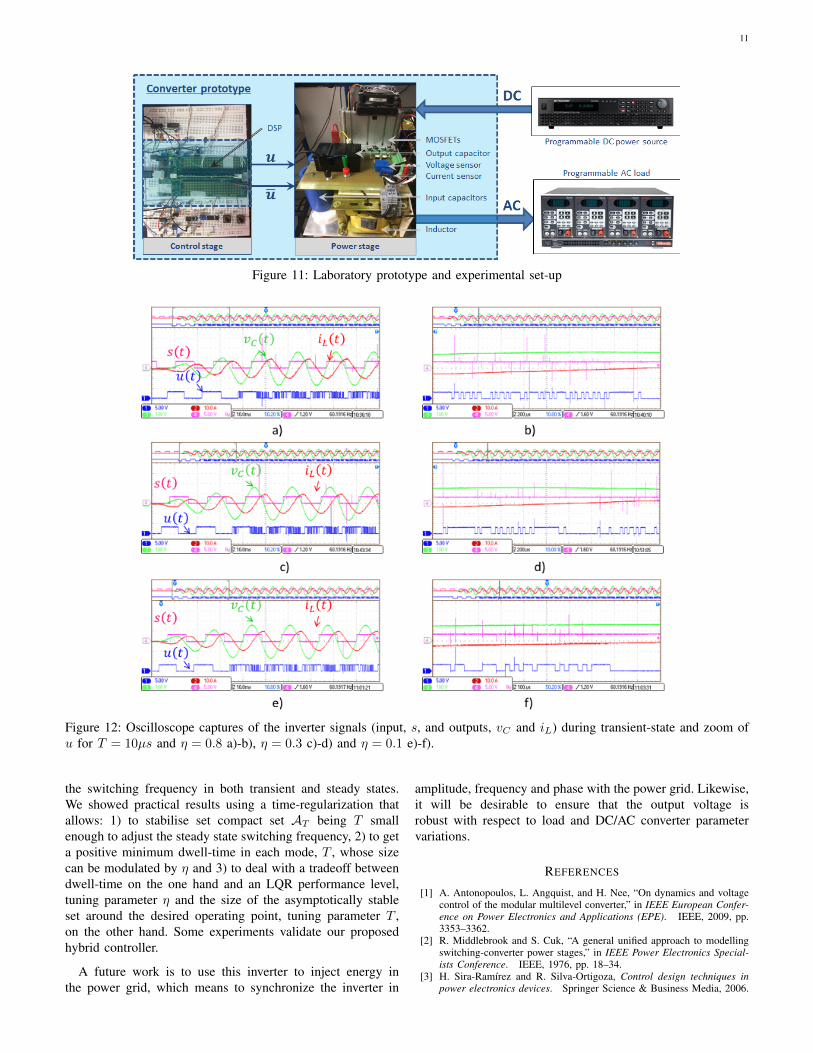
Figure 11 shows the prototype assembled with the measure-ment set-up.
The converter parameters appear in Table I and the desiredbehaviour in (43). The gains introduced by the sensors inthe measurements (which can condition the circuit) are com-pensated into the DSP algorithms. Then, the hybrid scheme(34) with matrices P and Q given above are implemented inthis DSP, and it is configured to have an internal interruptiondefining the sampling time in 10µs. This time is used to
generate a minimum dwell-time.
A. Performance evaluation for different values of η
First, we experimentally validate the efficiency of the hybridscheme (34) w.r.t. η, which conditions the transient time, asshown in Fig. 7. For this one, several experimental tests wereperformed in the prototype in nominal conditions of inputvoltage and load, for η = 0.1, 0.3, 0.8 and T = 10µs. Notethat these η values are according simulation results Fig. 7. Asshown in Fig. 12, system reaches the steady state in frequency,phase and amplitude before 50ms. The signal s(t) is obtainedfrom a digital output of the DSP and represents the polarityof the internally generated sinusoidal reference for vC (3V ifsignal is positive and 0V if signal is negative). Remark that theswitching frequency decreases as η diminishes, as is shown insimulation (see Fig. 8).
B. Steady-state performance for different values of T
Now, we validate the hybrid scheme (34) for different min-imum dwell times in steady state, T = 50µ, 100µ, 500µsand η = 0.1, applying several tests in nominal conditions.Figure 13 shows the steady state behaviour for different T . Wehighlight that the voltage and current output are practically thesame despite different T . However, the switching are reduced,as expected. These results show the dwell-time and UGASproperty for attractor AT properties given in Theorem 3, item1 and item 2, respectively. Moreover, we measured the THD ofthe output voltage using a Power Quality Analyzer Fluke 43Bwith constrained computations to 21 harmonics (1.26 kHz).THD values were obtained in a range between 1.0% and 1.3%,presenting the best result for η = 0.1 and T = 100µs (see Fig.14.c). In order to complement this result, a FFT analysis withextended bandwidth was performed using PSIM simulationsfor the same values of η and T obtaining THD values in arange between 1.8% and 3.5% and presenting the best resultfor η = 0.1 and T = 100µs. This means that for higher valuesof T , it is expected that THD increases due to the absence ofcommutations during a relevant slot time. This fact is veryimportant for low performance devices.
Moreover, we measured the inverter THD1, whose valuesare obtained in a range between 1.0% and 1.3% using aPower Quality Analizer Fluke 43B. The best measurementwas obtained for η = 0.1 and T = 100µs (see Fig.14 c).This means that for higher T or smaller η the THD increasesdue to the absence of switching during a relevant slot time.This fact is very important for low-cost devices, i.e. for lowperformance devices.
IX. CONCLUSIONS AND FUTURE WORK
In this work, we proposed a controller following a HDSframework for a dc-ac converter composed of continuousvariables (current and voltage) and discrete variables (stateof switches), whose main problem is to track a sinusoidalreference. The main advantage of this method is to manage
1The Total Harmonic Distortion (THD) is an output signal correspondingto a quality indicator of electronic converters
11
Figure 11: Laboratory prototype and experimental set-up
Figure 12: Oscilloscope captures of the inverter signals (input, s, and outputs, vC and iL) during transient-state and zoom ofu for T = 10µs and η = 0.8 a)-b), η = 0.3 c)-d) and η = 0.1 e)-f).
the switching frequency in both transient and steady states.We showed practical results using a time-regularization thatallows: 1) to stabilise set compact set AT being T smallenough to adjust the steady state switching frequency, 2) to geta positive minimum dwell-time in each mode, T , whose sizecan be modulated by η and 3) to deal with a tradeoff betweendwell-time on the one hand and an LQR performance level,tuning parameter η and the size of the asymptotically stableset around the desired operating point, tuning parameter T ,on the other hand. Some experiments validate our proposedhybrid controller.
A future work is to use this inverter to inject energy inthe power grid, which means to synchronize the inverter in
amplitude, frequency and phase with the power grid. Likewise,it will be desirable to ensure that the output voltage isrobust with respect to load and DC/AC converter parametervariations.
REFERENCES
[1] A. Antonopoulos, L. Angquist, and H. Nee, “On dynamics and voltagecontrol of the modular multilevel converter,” in IEEE European Confer-ence on Power Electronics and Applications (EPE). IEEE, 2009, pp.3353–3362.
[2] R. Middlebrook and S. Cuk, “A general unified approach to modellingswitching-converter power stages,” in IEEE Power Electronics Special-ists Conference. IEEE, 1976, pp. 18–34.
[3] H. Sira-Ramırez and R. Silva-Ortigoza, Control design techniques inpower electronics devices. Springer Science & Business Media, 2006.

12
Figure 13: Oscilloscope captures of the inverter signals (input, s, and outputs, vC and iL) in the steady state and zoom of ufor η = 0.1 and T = 50µs a)-b), T = 100µs c)-d) and T = 500µs e)-f).
Figure 14: THD measurements: a) η = 0.1 and T = 10µs; b)η = 0.1 and T = 50µs; c) η = 0.1 and T = 100µs; and d)η = 0.1 and T = 500µs
[4] M. Senesky, G. Eirea, and T. J. Koo, “Hybrid modelling and controlof power electronics,” in International Workshop on Hybrid Systems:Computation and Control. Springer, 2003, pp. 450–465.
[5] C. Sreekumar and V. Agarwal, “A hybrid control algorithm for voltageregulation in dc–dc boost converter,” IEEE Trans. on Industrial Elec-
tronics, vol. 55, no. 6, pp. 2530–2538, 2008.[6] G. S. Deaecto, J. C. Geromel, F. Garcia, and J. Pomilio, “Switched
affine systems control design with application to DC–DC converters,”IET control theory & applications, vol. 4, no. 7, pp. 1201–1210, 2010.
[7] C. Albea Sanchez, G. Garcia, and L. Zaccarian, “Hybrid dynamicmodeling and control of switched affine systems: application to dc-dcconverters,” in proc. IEEE Conference on Decision and Control (CDC),2015, pp. 2264–2269.
[8] J. Chai and R. G. Sanfelice, “A robust hybrid control algorithm for asingle-phase dcac inverter with variable input voltage,” in proc. IEEEAmerican Control Conference (ACC), 2014, pp. 1420–1425.
[9] L. Torquati, R. Sanfelice, and L. Zaccarian, “A hybrid predictive controlalgorithm for tracking in a single-phase dcac inverter,” in proc. IEEEControl Technology and Applications (CCTA), 2017, pp. 904–909.
[10] C. Albea Sanchez, O. Santos, D. Z. Prada, F. Gordillo, and G. Garcia,“Hybrid control scheme for a half-bridge inverter,” IFAC ProceedingsVolumes, vol. 50, no. 1, pp. 9336–9341, 2017.
[11] B. A. Francis, “The linear multivariable regulator problem,” SIAMJournal on Control and Optimization, vol. 15, no. 3, pp. 486–505, 1977.
[12] R. Goebel, R. Sanfelice, and A. Teel, Hybrid Dynamical Systems:modeling, stability, and robustness. Princeton University Press, 2012.
[13] D. Liberzon and A. Morse, “Basic problems in stability and design ofswitched systems,” IEEE Control Systems Magazine, vol. 19, no. 5, pp.59–70, 1999.
[14] C. Prieur, A. R. Teel, and L. Zaccarian, “Relaxed persistent flow/jumpconditions for uniform global asymptotic stability,” IEEE Trans. onAutomatic Control, vol. 59, no. 10, pp. 2766–2771, October 2014.
[15] M. Corless and A. Frazho, Linear systems and control: an operatorperspective. CRC Press, 2003.
[16] A. Seuret, C. Prieur, S. Tarbouriech, A. Teel, and L. Zaccarian, “Anonsmooth hybrid invariance principle applied to robust event-triggereddesign,” Submitted to IEEE Transactions on Automatic Control. See also:https://hal.archives-ouvertes.fr/hal-01526331/.
[17] R. G. Sanfelice, D. Copp, and P. A. Nanez, “A toolbox for simulation ofhybrid systems in Matlab/Simulink: Hybrid equations (HyEQ) toolbox,”in Hybrid Systems: Computation and Control Conference, 2013.